Abstract
Rice serves as the staple food for over 50% of the global population. Remotely-sensed based estimation of the gross primary production (GPP) and evapotranspiration (ET) of rice paddy fields is essential to assess global food security. In this study, we tested the application of a recently proposed remotely-sensed based water-carbon coupled model (PML-V2) in the lower reaches of the Poyang Lake plain, which is one of the nine production bases for crops in China. Evaluation using the eddy covariance measurements showed that, after parameter localization, the model reproduced the seasonal variations of GPP and ET for both the early rice and the late rice. The model performed reasonably well in the validation period because the key parameters (e.g., the quantum efficiency and the stomatal conductance coefficient) exhibited predictable seasonal variations. At the regional scale, the spatial distribution in multi-year GPP of rice (1365 ± 326 gCm−2year−1) can be explained by the vegetation cover fraction (R2 > 0.9); in comparison, the multi-year ET (1003 ± 65 mm/year) exhibits smaller spatial variations due to the high evaporation rate of the saturated soil surface of paddy fields. The water use efficiency of rice in this region varies around 1.35 gC/kgH2O with a standard deviation of 0.30. Our study shows that GPP and ET of rice can be estimated by remote sensing models without detailed crop management information, which is usually unavailable at regional scales.
1. Introduction
The fast-growing population is driving a fast-growing need in the food supply globally. In 2050, the increase of new cropland is projected to be about 1 billion ha [1], and the food production needs to be 70% higher to meet the caloric requirements of the global population [2]. Among all the staple foods, rice is a particularly important one because it feeds over 50% of the population worldwide [3]. Therefore, accurate estimation of rice yield and its water use, especially in the Asian monsoon region in which over 90% of the rice grows [4], is essential to guarantee global food security and sustainable development.
With the development of remote sensing techniques, numerous crop models [5] and statistical models [6] have assimilated the remotely sensed vegetation information to estimate regional crop yields [7]. For example, Sasai et al. [8] estimated the spatial and temporal variations in the rice productions in Japan with a diagnostic biosphere model and the Moderate Resolution Imaging Spectroradiometer (MODIS) leaf area index (LAI) product. The point-scale evaluation showed that, after introducing the harvest and soil oxidation-reduction processes, the root mean square errors were reduced to 27.31 gCm−2month−1 and 36.33 gCm−2month−1 for gross primary production (GPP) and net ecosystem production (NEP), respectively [8]. Other diagnostic models, such as the light use efficiency (LUE) model [9] and the light–response curve model [10] that were proposed to estimate ecosystem GPP without parameterizing the crop management information and the process at the vegetation–soil interface, were also widely used in the regional estimation of crop yields, for example, for the maize ecosystem [11], the wheat-maize rotating system [12], and rice paddy fields [13,14].
Irrigated croplands consume most of the precipitation by evapotranspiration (ET) [15] and therefore have strong feedback to the terrestrial hydrology and the near-surface atmosphere [16,17]. Compared to other crops and natural vegetation, the ET of the paddy field is generally much higher [18]. For example, Zhao et al. [19] reported that the ratio between ET and net radiation increases from 0.6 to 0.8 when a marshland was turned into a rice paddy field in the northeast region of China. Similarly, ET of rice takes up 63–67% of the total ET during the growing season for a rice-wheat rotation site in Nanjing, Eastern China [20]. Therefore, accurate estimation of regional ET for rice is essential for water management and sustainable agricultural development. The ET of rice can be estimated using the Priestley–Taylor (PT) method [21] or the Penman–Monteith model [22,23]. For example, Qiu et al. [24] examined the sensitivity of rice paddy ET to varying patterns of warming using a modified PT model in the East Asian monsoon regions. Xu et al. [25] estimated rice ET under water-saving irrigation by the PM model after calibrating the canopy resistance model parameters, in which LAI is used to scale up the stomatal conductance for water vapor from the leaf scale to the canopy scale.
To correctly assess the water use efficiency of crops, the rates of photosynthesis and transpiration of vegetation are usually estimated in a coupled way [26,27] because both carbon dioxide and water vapor go through leaves via the stomata. In addition, the stomatal conductance is sensitive to the photosynthesis rate [28]. Recently, Zhang et al. [29] and Gan et al. [30] proposed a routinely applicable water-carbon coupling model (PML-V2), which combines the carbon and vapor fluxes through the response of the canopy conductance to the photosynthesis rate. The PML-V2 model estimates GPP and ET using the light–response curve method and the PM model, respectively. Although the PML-V2 model has been tested at 95 EC sites globally [29], the usage of the model is seldomly evaluated for rice paddy fields. In this paper, based on eddy covariance (EC) data from a double-cropping rice paddy field in the lower reaches of the Poyang Lake basin, China, we intend to (1) test the usage of the PML-V2 model for a double-cropping rice paddy ecosystem in this area, (2) study the differences in key parameters of the model (light–responses, canopy conductances, and water–carbon coupling characteristics) between early rice and late rice, and (3) upscale the in situ GPP, ET, and water use efficiency (WUE) to the regional scale in the lower reaches in the Poyang Lake plain using the PML-V2 model.
2. Study Site and Data Processing
2.1. Study Site
Our study area is located in the lower reaches of the Poyang Lake plain (Figure 1), which is one of the nine production bases for crops in China. Characterized as the humid subtropical climate, the annual mean air temperature is 17.5 °C, and the mean annual precipitation is 1635.9 mm for the Poyang Lake basin for 1960–2010 [31,32]. The major rain season of this area is April to June, and precipitation decreases sharply after July [32]. In this paper, we applied the model at a regional scale (28°–29°N, 115.7–116.7°E) (Figure 1), where rice paddy fields occupy over 45% of the total land coverage, as shown in Figure 1. In addition, the selected area mainly contains the rice pixels that are near Poyang Lake, and the pixels in the Ganjiang and Fuhe watersheds, which are two major sub-watersheds of the Poyang Lake basin.
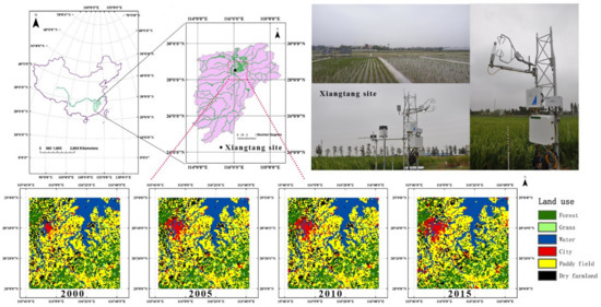
Figure 1.
Location of the study area, flux site, and the land cover in 2000, 2005, 2010, and 2015 in this area.
Rice is the main crop in the Poyang Lake basin, where dual cropping systems are prevalent. The early rice is generally growing from late March to middle July, and the late rice is generally growing from middle July to late October. After the late rice is harvested, herbaceous plants, such as the Chinese milk vetch, are usually grown to maintain the fertility of the land. The typical cropping system and management measures [33] in this area are summarized in Table 1. In this paper, we will evaluate the performances of the PML-V2 model in simulating the GPP and ET at the Xiangtang station (28°26′25″N, 116°00′01″E), which belongs to the Jiangxi Central Station of the Irrigation Experiment. Daily meteorological conditions and 8 day NDVI at the Xiangtang station were shown in Figure 2.

Table 1.
The cropping system and management measures at the Xiangtang station.
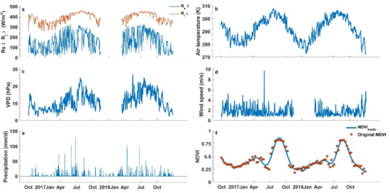
Figure 2.
Daily meteorological conditions and 8 day NDVI at the Xiangtang station, (a) the downward shortwave and longwave radiation, (b) air temperature, (c) vapor pressure deficit, (d) wind speed, (e) precipitation and (f) NDVI. The smoothed NDVI curve was obtained by the Hants method (NDVIhants).
2.2. Eddy Covariance Measurements and Meteorology Data at the Xiangtang Station
Up to date, the eddy-covariance technique has been the standard method in the ET and GPP measurements at scales of 102–103 m [34]. To measure the fluxes of sensible heat, latent heat, and CO2, we have set up an open-path eddy covariance system (Li-COR 7500) at a height of 2.5 m since October 2016 at the Xiangtang station. The three-dimensional wind velocities and CO2/H2O concentrations were recorded by a datalogger (model CR3000, Campbell Scientific, Inc., Logan, UT, USA) at a frequency of 10 Hz.
Other microclimate variables were measured as 30 min averages, including net radiation (Rn) (CNR4, Kipp and Zonen, Delft, The Netherlands), air temperature (Ta), and relative humidity (RH) (HMP155A, Vaisala, Inc., Vantaa, Finland), wind speeds (U) and wind direction (WD) (model 03002, RM Young, Inc., Dundee, MI, USA), and precipitation (model 52202, RM Young, Inc.). The soil heat fluxes (model HFP01SC, Campbell Scientific, Inc.) were measured at 0.05 m below the soil surface. All data were collected by a CR3000 datalogger as 30 min averages. The data were selected from October 2016 to December 2018, except from 16 November 2017 to 15 March 2018, due to an instrument malfunction. The data were divided into 18 periods according to the growing stages of early rice and late rice, as shown in Table 1.
We used the EddyPro software v6.1.0 (www.licor.com/eddypro, accessed on 15 December 2019) to process the high-frequency raw data. After the 30-min scale fluxes were calculated using the high-frequency measurements in the air temperature, humidity, CO2, and three-dimensional wind velocity, the post-field data processing program was developed following FLUXNET’s standard procedures [35]. The main data processing steps on the 30-min scale fluxes included spike removal [36], double coordinate rotation [37], frequency response corrections [38,39], and WPL corrections [40] for the air density fluctuations. The data quality check followed the method in Foken et al. [36], and the low-quality data were discarded in this study. Approximately 18.7% of the half-hour data points were removed as a result of a malfunction of the sensors, rain/fog influence, calibrations, and quality checks.
The net ecosystem exchange (NEE) measurements of carbon dioxide are then decomposed into GPP and Reco (Respiration of the ecosystem) using the nighttime-based partition method [41,42], in which the Reco = f(Ta) relationship is established using the nighttime NEE data. The daytime Reco is then estimated using the Reco = f(Ta) relationship and daytime Ta, and therefore GPP during daytime is then estimated as the difference between daytime NEE and daytime Reco. The surface energy balance closure at the Xiangtang station was 71% on a daily scale. The heat storage correction on soil heat flux was calculated using the method of Heusinkveld et al. [43], and the energy balance correction on H and LE was performed using the Bowen-ratio method [44].
Data gaps were filled by three methods [45], including linear interpolation (gap < 2 h), look-up table method (gap within 2–12 h), and the multi-regression method (gap > 12 h). Missing net radiation, air temperature, relative humidity, and wind speed data were filled by data collected at the national standard meteorological station located near the Xiangtang station.
2.3. Regional Data
We used the China Meteorological Forcing Dataset (CMFD) [46,47] for regional climate forcing, which is at the spatial resolution of 0.1°, and temporal resolution of 3 h. CMFD was produced by merging a variety of data sources, including CMA (China Meteorological Administration) weather station observation data, TRMM satellite precipitation analysis data (3B42), GEWEX-SRB downward shortwave radiation data, the Modern Era-Retrospective Analysis for Research and Applications (MERRA) (surface pressure), and GLDAS data (wind, air temperature, relative humidity, air pressure, and precipitation) [46].
The NDVI and albedo data used in this study were derived from the MODIS products MOD13Q1/MYD13Q1 and MCD43A3, which have a spatial resolution of 250 m and 1000 m, respectively. Due to the existence of cloud cover, the MODIS NDVI/Albedo values are often missing or underestimated. To remove the outliers and fill the missing gaps in the original time series, we used the technique of Harmonic Analysis of Time Series (HANTS) [48]. The LAI was estimated using the NDVI data. LAI is estimated from NDVI in this study due to its relatively high spatial resolution (250 m). First, vegetation coverage fc is estimated using the NDVI, i.e., fc = (NDVImax − NDVI)/(NDVImax − NDVImin), where NDVImax and NDVImin are taken as 0.95 and 0.01, respectively. LAI is then inverted using the relationship between the LAI and vegetation coverage, i.e., fc = 1 − exp(−0.6 ∗ LAI) [49,50]. Land cover data in the years 2000, 2005, 2010, and 2015 were provided by the National Earth System Science Data Center of China (http://auth.geodata.cn, accessed on 30 June 2020). All data were resampled to 250 m and a daily scale.
3. The PML-V2 Model
The PML-2 model is an updated version of the Penman-Monteith-Leuning (PML) model [22,23,51], which estimates ET using the PM equation with a Jarvis–Stewart type conductance model [52,53]. The Jarvis–Stewart type conductance model estimates the leaf conductance to CO2/vapor by multiplying the species-dependent maximum conductance values with scaling factors that reflect the constraints of radiation, leaf properties, and water supply conditions [50,54]. To make the conductance model more physically realistic, Gan et al. [30] replaced the semi-empirical Jarvis–Stewart model with a biophysical one [55] that reflects the control of photosynthesis, concentrations of CO2, and water vapor on leaf stomatal conductance.
The major components of the PML-V2 model, i.e., the estimation of GPP using the light–response curve, of ET using the PM model, and the coupling between GPP and ET using the biophysical conductance model, are introduced as follows. For more details, please refer to Gan et al. [30] and Zhang et al. [29].
3.1. The Estimation of GPP
In PML-V2, the photosynthesis rate of leaves, Ag, estimated from radiation intensity (I, µmol m−2s−1) and the concentration of CO2 (Ca, ppm) using a rectangular hyperbola function [10] are shown as follows:
where β is the quantum efficiency, defined as the initial slope of the response curve of assimilation rate of leaves to light (µmol CO2 (µmol PAR)−1), η is the carboxylation efficiency, defined as the initial slope of the response curve of assimilation rate of leaves to CO2 (µmol m−2 s−1 (µmol m−2 s−1)−1), Am (µmol m−2 s−1) is the maximum photosynthetic rate obtained when both I and Ca are saturated, which is temperature-dependent [56,57], shown as follows:
where Vm,25 is a parameter that has the same dimension with Am, and a and b are temperature coefficients, which are taken as 0.031 and 0.115, respectively [58]. The PML-V2 model estimates the canopy carbon assimilation rate Acg by integrating the Ag of leaves to the canopy scales using LAI, shown as the following:
where
The ecosystem GPP is finally determined using Acg and a constraint function that reflects the effect of atmospheric dryness (Da, vapor pressure deficit, kPa) on GPP, where Dmax and Dmin are parameters.
3.2. The Estimation of ET
ET includes transpiration from leaf stomata (T), evaporation from the soil (Es), and wet leaf surfaces (Ei) [59,60]. T is estimated using the Penman–Monteith model [22,23], shown as the following:
where (--), Δ is the slope of the saturated vapor pressure to the air temperature (kPaK−1), γ is the psychrometric constant (kPa K−1), and A is the available energy (net radiation Rn minus soil heat flux G, MJ m−2 d−1); ρ is the density of air (g m−3); cp is the specific heat of air at constant pressure (J g−1 K−1); Ga is the aerodynamic conductance (m s−1), and Gc is the canopy conductance (m s−1). Rn was estimated as the difference between the incoming and outgoing radiation at the surface, i.e., = (1 − α) ∗ Rs + (Rli − Rlo), where α is the albedo, Rs is the incoming shortwave solar radiation, Rli is the incoming longwave radiation, and Rlo is the outgoing longwave radiation.
The soil evaporation (Es) is estimated using the PT equation, shown as follows:
where the fraction coefficient f varies from 0 to 1 when the soil surface is changing from completely dry to wet. In PML-V2, f is determined by the relative magnitude between the accumulated precipitation and soil equilibrium evaporation in the previous 32 days [29]. In this study, we added a parameter αs to account for the saturation property of the rice paddy field because a previous study showed that, on average, evaporation of wetland in this region is 1.26 times the equilibrium evaporation [61]:
The evaporation from wet leaf surfaces (ETi) is expressed as
with
where Pwet is the reference threshold rainfall amount if the canopy is wet (mm d−1), fER is the ratio of average evaporation rate over average precipitation intensity storms (unitless), fER = fV ∗ F0. fV is the fractional area covered by intercepting leaves (unitless), and P is the daily precipitation (mm d−1). Sl and F0 are two free parameters for Ei. Sl is the specific canopy rainfall storage capacity per unit leaf area, and F0 is the specific ratio of average evaporation rate over average rainfall intensity during storms. For more details on the estimation of Ei, please refer to the supplementary material of Zhang et al. [29].
3.3. Biophysical Conductance Model
The leaf conductance gs can be written as a function of Ag, Ca, and Da [55]:
The PML-V2 model estimates the canopy conductance Gc by integrating gs to the canopy scale, shown as follows:
3.4. Model Calibration and Validation
To evaluate the PML-V2 model, we calibrated the model parameters for each growing stage (P3, P4,…, P9, in Table 1) separately, in 2017, and tested the model performances in 2018, where parameters in each growing stage (P11, P12,…, P17, in Table 1) in 2018 were taken as those in the periods of P3, P4,…, P9, respectively, in 2017. The definitions and ranges of all parameters of the PML-V2 model are summarized in Table 2. For each period, we first calibrated the parameters of Vm25, β, η, Dmin, Dmax, and KQ by minimizing the RMSE in GPP predictions and then calibrated the rest of the parameters by minimizing the RMSE in ET predictions. In addition, to explore the seasonal variations in the model parameters that are related to the light responses, canopy conductances, and water-carbon coupling characteristics of the rice paddy ecosystem, we also calibrated the model in each period of early rice and late rice in both 2017 and 2018 (P3, P4,…, P9 and P11, P12,…, P17), separately.
Table 2.
Summary of parameters used in the PML-V2 model.
4. Results
4.1. GPP and ET Fluxes of RICE Paddy Field at the Site-Level
As shown in Figure 3, the GPP of the rice paddy field at the Xiangtang station exhibited seasonal variations with two peaks, corresponding to the growth of the early rice and late rice throughout the year. For the early rice, the GPP peaks at the middle/late stages, i.e., 12.02 gCm−2day−1 and 13.73 gCm−2day−1 for 2017 and 2018, respectively (Figure 3). On average, the GPP of early rice was 4.78 gCm−2day−1 and 6.02 gCm−2day−1 for 2017 and 2018, respectively (Table 3). In contrast, the average GPP of late rice, i.e., 8.70 gCm−2day−1 and 7.91 gCm−2day−1 for 2017 and 2018, respectively, were much larger than those for the early rice. In addition, compared to the early rice, GPP of the late rice increases more rapidly at the beginning of the growing stage (Figure 3); therefore, GPP peaks at the middle stages for the late rice, and the peaks were larger than those for the early rice, i.e., 16.64 gCm−2day−1 and 14.45 gCm−2day−1 for 2017 and 2018, respectively. The faster growth rate in the beginning stage of the late rice than of early rice may be due to the fact that crops usually grow slower at lower temperatures. Ta at the beginning stage (since 24 March) of the early rice was 16.7–21.8 °C lower than that at the beginning stage (since 15 July) of the late rice (Figure 2).

Figure 3.
Time series of (A) daily GPP and (B) ET at the Xiangtang station.
Table 3.
Daily average values of GPP, ET, and H for the early rice and late rice in 2017 and 2018.
Compared to the GPP, ET of the rice paddy has only one peak (Figure 3). There appear to be two peaks in 2017; however, the low ET in late June and the first few days in July in 2017 were mainly due to cloudy and rainy conditions, in which the relatively small solar radiation (Figure 2) was probably the limiting factor for ET. As shown in Table 3, ET consumed most of the available energy because the Bowen ratio (the ratio between sensible and latent heat) of the paddy field was only about 0.1 for both the early rice and late rice. On average, ET for the late rice is generally larger than for early rice. However, the ecosystem water use efficiency (WUE), which is defined as the ratio between the GPP and ET, i.e., 1.86 gC/kgH2O and 1.59 gC/kgH2O for late rice, was still higher than those, i.e., 1.41 gC/kgH2O and 1.48 gC/kgH2O for early rice, in 2017 and 2018, respectively.
4.2. Seasonal Variations in the Key Parameters of the PML-V2 Model for the Early Rice and Late Rice Ecosystems
To reveal the seasonal variations in the key characteristics that govern the GPP, transpiration, and soil evaporation process, mainly including the light-response (β) and CO2-response (η) properties, the maximum catalytic capacity of Rubisco (Vm25), the canopy conductance coefficient (m), and the soil evaporation coefficient (αs), we calibrated the parameters of the PML-V2 model in every growing stage separately (Table 2) for both the early rice and the late rice ecosystems, as shown in Table 4.
Table 4.
The calibrated parameters of the PML-V2 model at different growing stages (Table 1) of early rice and late rice in 2017 and 2018.
The parameters that govern the GPP estimation differ for the early rice and late rice. The carboxylation efficiency η for the early rice increases as the crop grows, from less than 0.02 µmol m−2 s−1 (µmol m−2 s−1)−1 to nearly 0.15 µmol m−2 s−1 (µmol m−2 s−1)−1 at its grouting stage (Figure 4) and then decreases. In addition, the maximum catalytic capacity of Rubisco, Vm25, and the quantum efficiency β generally exhibited a similar change pattern as the GPP (Figure 4c) during the early rice period. Compared to the early rice case, the change patterns in parameters for the late rice periods did not typically coincide with the GPP. In addition, the inter-annual variations in parameters are larger for late rice. For example, the late rice in 2017 was less sensitive to light and CO2, with generally much smaller quantum efficiency β and the carboxylation efficiency η than those for late rice in 2018.
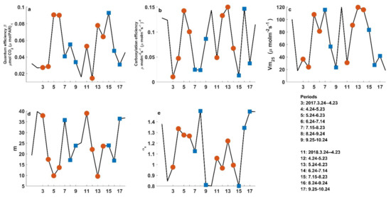
Figure 4.
Key parameters in the PML-V2 model in different stages of early rice (red) and late rice (blue). (a) Quantum efficiency β; (b) Carboxylation efficiency η; (c) notional maximum catalytic capacity of Rubisco Vm25; (d) Stomatal conductance coefficient m, and (e) Soil evaporation coefficient αs.
The parameters that govern the transpiration estimation for the early rice and late rice showed similar averages and variability (Figure 4d,e). For example, the parameter m, which represents the sensitivity of the canopy conductance to the photosynthesis rate, is generally 20–25 on average for both the early rice and late rice. However, the parameter m showed smaller deviations from its mean value in the early rice period than in the late rice period. In addition, the parameter m generally decreases as GPP increases, indicating that the canopy conductance is more sensitive to GPP when GPP is smaller. The soil evaporation coefficient αs varies around 1.1 for both the early rice and late rice periods.
4.3. Model Evaluation at the Xiangtang Station
For the calibration period (2017), model performances were reasonably good, with predictions in the GPP and ET matching the dynamic characteristics and the peaks of measured GPP and ET (Figure 5). The RMSE in GPP generally peaks in the stage of the resume growth before jointing; however, the RMSE is generally less than 50% of the mean GPP (Figure 6). In addition, the mean bias in the GPP for the early rice is close to 0 on average and relatively small compared to the mean GPP during the growing period of early rice. Compared to GPP, the RMSE in ET predictions from the PML-V2 model is even smaller, about 10% of the mean ET. The overall good performances in the simulations of both GPP and ET indicate that the PML-V2 model is capable of predicting crop yield and its water use for rice paddies if the proper parameters are used.
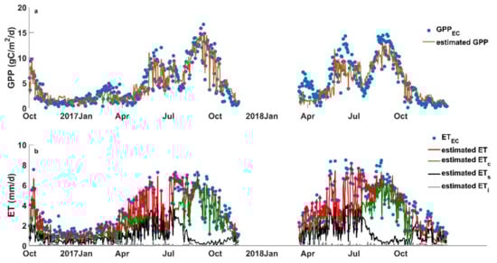
Figure 5.
Daily predictions in (a) GPP and (b) ET components from the PML-V2 model when the parameters in 2017 were used for both 2017 and 2018 at the Xiangtang station.
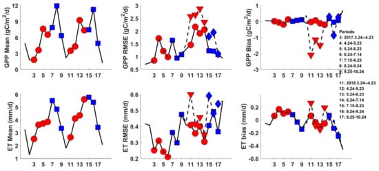
Figure 6.
Prediction accuracy from the PML-V2 model in different growing stages of early rice (red) and late rice (blue). The solid lines represent model simulations when the optimized parameters were used in each growing stage, and the dotted lines represent model simulations in 2018 when the parameters of 2017 were used.
To fully evaluate the PML-V2 model, we used the “calibration–validation” strategy and re-ran the model in 2018 using the parameters that were calibrated in 2017. The seasonal changes in GPP predictions generally coincided with the change patterns in the GPP measurements throughout the year in 2018; however, GPP was underestimated in the early rice stage (Figure 5a and Figure 6). Compared to the “optimized” simulations, where parameters were optimized in every growing stage in 2017 and 2018 (Figure 6), RMSE in GPP increased ~0.2–1.0 gCm−2d−1 when the model was run at the early rice period, and the mean bias reached over −2 gCm−2d−1 at the first growth stage of the early rice. In comparison, model simulations were much better for the late rice (Figure 5a and Figure 6). Compared to the GPP estimation, ET estimation in 2018 showed more robust results. The predictions in ET and its three components were generally consistent with the optimized simulations. RMSE in ET predictions increased only ~0.1–0.2 mm/day, and the mean bias was confined reasonably well.
4.4. Regional Estimation of GPP and ET Using the PML-V2 Model
We applied the PML-V2 model to estimate the regional (28–29°N, 115.7–116.7°E) distribution of GPP and ET in 2000, 2005, 2010, and 2015 at the spatial resolution of the NDVI data (0.0025°). The calibrated parameters, including those at different growing stages for the early rice and late rice at the Xiangtang Station, were used. Despite the relatively small extent of our study area (~104 km2), some of the meteorological conditions exhibit large spatial variations even on an annual time scale, especially for the specific humidity, the wind speed, and the precipitation (Figure 7 and Figures S1–S3). For example, annual precipitation ranges from 1400 mm to over 2200 mm across the region in 2005 (Figure S2). In addition, meteorological conditions exhibit inter-annual variations (Figure 7 and Figures S1–S3). For example, Ta increases in the 2000–2015 period. NDVI also increases, although the solar radiation peaked in 2005 and the precipitation was the largest in 2010.
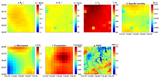
Figure 7.
Regional distribution of annual averages of meteorological variables and NDVI in 2010.
The estimated annual GPP of paddy rice (including early rice and late rice) was 1314 ± 286 gC m−2, 1358 ± 311 gC m−2, 1319 ± 314 gC m−2, and 1453 ± 359 gC m−2 in 2000, 2005, 2010, and 2015, respectively. No significant trend exists during the 2000–2015 period. The annual GPP showed large spatial variations, with the largest GPP in the southeast of the region and relatively small GPP in the west region (Figure 8). We further demonstrated the spatial variability of GPP (ET and WUE) using the violin plot (Figure 9), which combines the boxplot of GPP (ET and WUE) with its probability density distribution. As shown in Figure 9, the total amount of GPP for the early rice and late rice also exhibits small inter-annual variations but large spatial variations within a single year. The probability density distribution of GPP was generally symmetric (Figure 9), indicating that the mean value of GPP is close to the median value of GPP. The total amount of GPP of the early rice was 709 ± 167 gC m−2, 723 ± 174 gC m−2, 681 ± 164 gC m−2, and 707 ± 183 gC m−2, and the total amount of GPP of the late rice was 605 ± 149 gC m−2, 635 ± 167 gC m−2, 638 ± 172 gC m−2, and 746 ± 200 gC m−2 in 2000, 2005, 2010, and 2015, respectively. The GPP of the early rice showed less spatial variability than that of the late rice. Spatially, GPP was highly correlated (correlation coefficient r > 0.96) with the NDVI distribution for both the early rice and late rice periods (Figure 10). In contrast, GPP for the early rice was weakly correlated with the meteorological conditions. For the late rice, GPP was negatively correlated with Ta (r = −0.26).
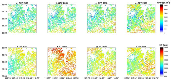
Figure 8.
Regional predictions in annual sums of GPP and ET in 2000, 2005, 2010, and 2015.
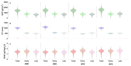
Figure 9.
Violin plots for regional GPP (a), ET (b), and WUE (c). The boxplot and the probability density function in the violin plot were drawn using the spatially distributed grid cells of the accumulated GPP and ET (and therefore WUE) in the early rice period, late rice period, and both of the periods.
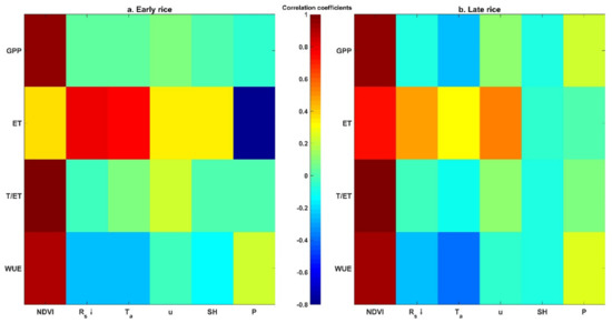
Figure 10.
Correlation coefficients r between the predicted GPP, ET, WUE, and the environmental variables, including the NDVI, downward shortwave radiation (Rs↓), air temperature (Ta), wind speed (u), specific humidity (SH), and precipitation (P) for the early rice (a) and late rice (b).
The estimated annual ET of paddy rice (including early rice and late rice) was 988 ± 49 mm, 1075 ± 56 mm, 968 ± 46 mm, and 984 ± 48 mm in 2000, 2005, 2010, and 2015, respectively. No significant trend exists during the 2000–2015 period. Compared to the GPP, the estimated annual ET was also relatively large, but not always the largest, in the southeast of the region. For example, ET was the largest in the northern part of the region in 2005 due to the heavy rain in this area (Figure S2). ET exhibits smaller spatial variations compared to that of GPP (Figure 9). The probability density distribution of ET was also generally symmetric (Figure 9). The total amount of ET of the early rice was 517 ± 19 mm, 551 ± 25 mm, 449 ± 15 mm, and 488 ± 22 mm, and the total amount of ET of the late rice was 471 ± 33 mm, 524 ± 34 mm, 518 ± 33 mm, and 496 ± 29 mm in 2000, 2005, 2010, and 2015, respectively. ET for the early rice was not strongly correlated with NDVI (r = 0.37). In contrast, ET was highly correlated with the solar radiation (r = 0.80) and air temperature (r = 0.77) for the early rice (Figure 10). ET for the late rice was highly correlated with NDVI (r = 0.73), followed by wind speed (r = 0.54) and solar radiation (r = 0.48).
The median value of WUE is ~1.40 gC/kgH2O for both the early rice and late rice. Despite the relatively small spatial variations in ET, the WUE exhibits larger variations than those of GPP and ET (Figure 9). WUE is generally higher in conditions with larger vegetation coverage, with correlation coefficients with NDVI equal 0.90 and 0.93 for the early and late rice, respectively. However, WUE is negatively correlated with Rs, Ta, u, and specific humidity.
5. Discussion
Rice is the major crop type in our study area. Compared to other crops, the WUE of rice is usually relatively low. For example, Wang et al. [62] reported that, among the staple crops, the maize cropland has the highest WUE with 2.48 ± 0.69 gC/kgH2O, followed by winter wheat (2.00 ± 0.39 gC/kgH2O), soybean (1.92 ± 0.52 gC/kgH2O), and paddy rice (1.88 ± 0.63 gC/kgH2O). Our results showed that WUE for rice at the Xiangtang station ranges from 1.41 gC/kgH2O to 1.86 gC/kgH2O for the early rice and late rice, which was consistent with the review of Wang et al. [62]. The relatively low WUE for rice is partly because the ET of rice is usually large due to the (nearly) constant saturation condition of the paddy fields. The Bowen ratio of the paddy field in our study was about only 0.1 for both the early rice and late rice (Table 3), indicating that ET consumes most of the net radiation of the land surface, which is consistent with other studies, e.g., the Bowen ratio of the flooded rice paddy fields in the Philippines is also only 0.14 on average [63,64]. Among the total ET, transpiration takes up ~50% on average in the growing stages of the early rice, and over 80% for the late rice (Figure 11). Therefore, the ecosystem WUE (WUEe) is close to the canopy WUE (WUEc) for the late rice, whereas the WUEc is much larger than WUEe for the early rice, especially in the stages from jointing to yellow ripen (Figure 11).
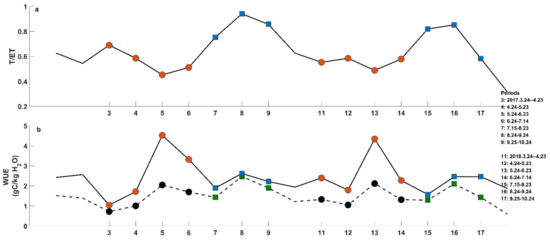
Figure 11.
T/ET (a) and WUE (b) in different stages of rice growing. In (a), red circles and blue squares represent T/ET for the early rice and late rice, respectively. In (b), red circles and blue squares represent the canopy WUE (WUEc = GPP/T) for the early rice and late rice, respectively; black circles and green squares represent the ecosystem WUE (WUEe = GPP/ET) for the early rice and late rice, respectively.
The accuracy of the PML-V2 model in simulating GPP and ET of rice is reasonably good compared to other modeling studies. For example, Zhang et al. (2020) estimated the photosynthetic rate of rice using a light–response curve model and found that R2 ranges from 0.77 to 0.96 at a daily scale when the multi-spectral reflectance data from an unmanned aerial vehicle were used. R2 from the PML-V2 GPP simulations was also larger than 0.90 in our study case if parameters were optimized in each growing stage. R2 was 0.72 for GPP during the validation period (2018) if the parameters in 2017 were used. As for ET estimation for paddy fields, Xu et al. (2017) proposed a Javis–Stewart type conductance model and successfully simulated rice ET using the conductance-based PM model at the Kunshan irrigation and drainage experiment station (31°15′15″N, 120°57′43″E), which is located to the northeast of the Xiangtang station (28°26′25″N, 116°00′01″E) and is also subject to a subtropical monsoon climate in the Taihu Lake region of China. After calibration, the model performed well with RMSE of 0.24 mm/d and 0.30 mm/d for 2014 and 2015, respectively, which is relatively small compared to the mean ET (3.52 mm/d) during the rice growth period (Xu et al., 2017). In comparison, the RMSE in ET predictions from the PML-V2 model is also less than 15% of the mean ET during the validation period (2018) if the parameters in 2017 were used.
Although similar modeling accuracy for GPP or ET has been achieved in previous studies, the advantage of the PML-V2 model is that the rates of photosynthesis and transpiration of vegetation are interconnected in the calculation process, which helps to correctly assess the WUE of an ecosystem and the canopy. However, we want to note that the reasonable performance of the model here relies on local calibration. In the paper of Zhang et al. (2019), parameters are fixed for all crops across the globe. Compared to their default values, e.g., the carboxylation efficiency (0.07 µmol m−2 s−1 (µmol m−2 s−1)−1), our study obtained similar values on average but with obvious seasonal variation. Other parameters, e.g., the stomatal conductance coefficient, m, varies around 20 in our study site, which is similar to that of the wetland (25.8) other than that of the crop (8.4) in Zhang et al. (2019).
We want to note that the PML-V2 model was evaluated using only one set of EC equipment at the Xiangtang site in our study area. However, because the study area is quite small, we assume that the parameters that were retrieved using the EC measurements at the Xiangtang site are representative of the characteristics of rice ecosystems in this area. Therefore, parameters of the PML-V2 model were assigned the same values for each rice grid in the study area. However, our results showed that GPP and ET of rice paddy fields exhibited substantial spatial variations (Figure 10 and Figure 11) because meteorological and land surface conditions were different for different grids. Moreover, simple relations are expected to exist between the multi-year daily values of GPP, ET, and the meteorological and land surface variables. Compared to the meteorological variables which were at 0.01° resolution, the NDVI data can be acquired at a much finer resolution (0.0025°), which was approximately equal to 250 m. Therefore, it is expected that the spatial distribution of estimated GPP was mainly correlated with the NDVI. The stepwise regression analysis showed that the NDVI can explain over 90% of the spatial variations in the multi-year daily values of GPP of the early rice. In addition, the slopes of NDVI in the regression equations for both the early rice and late rice were close to each other (14.14 v.s. 14.11). Compared to that of GPP, ET exhibited much smaller spatial variation due to the high evaporation rate of the saturated soil surface of paddy fields, which is comparable to the transpiration rate of the canopy; therefore, meteorological variables such as downward shortwave radiation, air temperature, and wind speed entered the regression equation. Besides GPP and ET, the stepwise regression also showed that, together with meteorological variables, the NDVI can explain over 90% of the spatial variations in the multi-year daily values of T/ET, and over 80% for those of WUE (Table 5).
Table 5.
Stepwise linear regression analysis for multi-year daily values of all gridded GPP (gC/m2/d), ET (mm/d), T/ET (--), and WUE (gC/kgH2O) for the early rice and late rice in the study area.
6. Conclusions
Estimating GPP and ET in a water–carbon coupling way is important to correctly assess the water use efficiency of crops. In this paper, the usage of the PML-V2 water-carbon coupling model was evaluated in the lower reaches of the Poyang Lake plain. As a diagnostic model, the PML-V2 model does not require detailed crop management information; however, the model performed reasonably well in simulating both the GPP and ET and therefore the WUE because the key parameters of the model exhibited predictable seasonal variations, and the NDVI is capable of indicating crop growth status. Our study shows that the PML-V2 model is feasible in regional estimates of rice GPP and ET in the sub-tropical climate.
The vegetation information (e.g., NDVI) is the most important input for regional application because of its fine spatial resolution. However, the uncertainty of vegetation information will propagate into the estimation of GPP, canopy conductance, and therefore canopy transpiration. The calibrated parameters are prone to NDVI uncertainty. In addition, due to the limited temporal resolution of the MODIS NDVI product (16 days), it is difficult to retrieve the start and end dates of the growth stages of the rice. In conclusion, vegetation information at finer spatial and temporal resolution is the key to the application of the PML-V2 model.
Supplementary Materials
The following are available at https://www.mdpi.com/article/10.3390/rs13173470/s1, Figure S1: Regional distribution of annual averages of meteorological variables and NDVI in 2000, Figure S2: Regional distribution of annual averages of meteorological variables and NDVI in 2005, and Figure S3: Regional distribution of annual averages of meteorological variables and NDVI in 2015.
Author Contributions
Conceptualization, G.G.; methodology, G.G. and X.Z.; formal analysis, G.G.; resources, Y.L., H.X., W.J.; data curation, X.F., H.Z. and Y.C.; writing—original draft preparation, G.G. and X.Z.; writing—review and editing, Y.L.; visualization, G.G.; supervision, Y.L.; project administration, Y.L. All authors have read and agreed to the published version of the manuscript.
Funding
Our research is jointly funded by the National Natural Science Foundation of China (42071054, 41971374, 51879255) and the Open Fund of State Key Laboratory of Remote Sensing Science (OFSLRSS202020).
Institutional Review Board Statement
The study was conducted according to the guidelines of the Nanjing Institute of Geography and Limnology, Chinese Academy of Sciences, and approved by the Nanjing Institute of Geography and Limnology, Chinese Academy of Sciences.
Informed Consent Statement
Not applicable.
Data Availability Statement
The data presented in this study are available on request from the corresponding author.
Acknowledgments
The MODIS data were downloaded from the NASA Goddard Space Flight Center (http://ladsweb.nascom.nasa.gov/data/, accessed on 10 June 2019).
Conflicts of Interest
The authors declare no conflict of interest.
References
- Tilman, D.; Balzer, C.; Hill, J.; Befort, B.L. Global food demand and the sustainable intensification of agriculture. Proc. Natl. Acad. Sci. USA 2011, 108, 20260–20264. [Google Scholar] [CrossRef] [Green Version]
- Alexandratos, N.; Bruinsma, J. World Agriculture: Towards 2030/2050—The 2012 Revision; No. 12–03ESA working paper; FAO: Rome, Italy, 2012. [Google Scholar]
- Food and Agriculture Organization of the United Nations. Teams on International Investment and Tropical fruits Trade and Market Division. Banana Market Review: Preliminary Results. Available online: http://www.fao.org/faostat/en/#data/QC (accessed on 30 July 2019).
- Li, C.; Mosier, A.; Wassmann, R.; Cai, Z.; Zheng, X.; Huang, Y.; Tsuruta, H.; Boonjawat, J.; Lantin, R. Modeling greenhouse gas emissions from rice-based production systems: Sensitivity and upscaling. Glob. Biogeochem. Cycles 2004, 18. [Google Scholar] [CrossRef]
- Campos, I.; Neale, C.M.; Arkebauer, T.J.; Suyker, A.E.; Gonçalves, I.Z. Water productivity and crop yield: A simplified remote sensing driven operational approach. Agric. For. Meteorol. 2018, 249, 501–511. [Google Scholar] [CrossRef]
- Kern, A.; Barcza, Z.; Marjanović, H.; Árendás, T.; Fodor, N.; Bónis, P.; Bognár, P.; Lichtenberger, J. Statistical modelling of crop yield in Central Europe using climate data and remote sensing vegetation indices. Agric. For. Meteorol. 2018, 260, 300–320. [Google Scholar] [CrossRef]
- Karthikeyan, L.; Chawla, I.; Mishra, A.K. A review of remote sensing applications in agriculture for food security: Crop growth and yield, irrigation, and crop losses. J. Hydrol. 2020, 586, 124905. [Google Scholar] [CrossRef]
- Sasai, T.; Nakai, S.; Setoyama, Y.; Ono, K.; Kato, S.; Mano, M.; Murakami, K.; Miyata, A.; Saigusa, N.; Nemani, R.R.; et al. Analysis of the spatial variation in the net ecosystem production of rice paddy fields using the diagnostic biosphere model, BEAMS. Ecol. Model. 2012, 247, 175–189. [Google Scholar] [CrossRef]
- Xiao, X.; Zhang, Q.; Braswell, B.; Urbanski, S.; Boles, S.; Wofsy, S.; Moore, B., III; Ojima, D. Modeling gross primary production of temperate deciduous broadleaf forest using satellite images and climate data. Remote Sens. Environ. 2004, 91, 256–270. [Google Scholar] [CrossRef]
- Thornley, J.H.M. Mathematical Models in Plant Physiology: A Quantitative Approach to Problems in Plant and Crop Physiology; Academic Press: Cambridge, MA, USA, 1977. [Google Scholar]
- Wang, Z.; Xiao, X.; Yan, X. Modeling gross primary production of maize cropland and degraded grassland in northeastern China. Agric. For. Meteorol. 2010, 150, 1160–1167. [Google Scholar] [CrossRef]
- Yan, H.; Fu, Y.; Xiao, X.; Huang, H.Q.; He, H.; Ediger, L. Modeling gross primary productivity for winter wheat–maize double cropping system using MODIS time series and CO2 eddy flux tower data. Agric. Ecosyst. Environ. 2009, 129, 391–400. [Google Scholar] [CrossRef]
- Boschetti, M.; Stroppiana, D.; Confalonieri, R.; Brivio, P.A.; Crema, A.; Bocchi, S. Estimation of rice production at regional scale with a Light Use Efficiency model and MODIS time series. Ital. J. Remote Sens. Riv. Ital. Telerilevamento 2011, 43, 63–81. [Google Scholar]
- Zhang, N.; Su, X.; Zhang, X.; Yao, X.; Cheng, T.; Zhu, Y.; Cao, W.; Tian, Y. Monitoring daily variation of leaf layer photosynthesis in rice using UAV-based multi-spectral imagery and a light response curve model. Agric. For. Meteorol. 2020, 291, 108098. [Google Scholar] [CrossRef]
- Liu, C.; Zhang, X.; Zhang, Y. Determination of daily evaporation and evapotranspiration of winter wheat and maize by large-scale weighing lysimeter and micro-lysimeter. Agric. For. Meteorol. 2002, 111, 109–120. [Google Scholar] [CrossRef]
- Leng, G.; Huang, M.; Tang, Q.; Sacks, W.J.; Lei, H.; Leung, L.R. Modeling the effects of irrigation on land surface fluxes and states over the conterminous United States: Sensitivity to input data and model parameters. J. Geophys. Res. Atmos. 2013, 118, 9789–9803. [Google Scholar] [CrossRef]
- Gan, G.; Liu, Y.; Sun, G. Understanding interactions among climate, water, and vegetation with the Budyko framework. Earth-Sci. Rev. 2020, 212, 103451. [Google Scholar] [CrossRef]
- Acreman, M.C.; Harding, R.J.; Lloyd, C.R.; McNeil, D.D. Evaporation characteristics of wetlands: Experience from a wet grassland and a reedbed using eddy correlation measurements. Hydrol. Earth Syst. Sci. 2003, 7, 11–21. [Google Scholar] [CrossRef] [Green Version]
- Zhao, X.; Huang, Y.; Jia, Z.; Liu, H.; Song, T.; Wang, Y.; Shi, L.; Song, C.; Wang, Y. Effects of the conversion of marshland to cropland on water and energy exchanges in northeastern China. J. Hydrol. 2008, 355, 181–191. [Google Scholar] [CrossRef]
- Qiu, R.; Liu, C.; Cui, N.; Wu, Y.; Wang, Z.; Li, G. Evapotranspiration estimation using a modified Priestley-Taylor model in a rice-wheat rotation system. Agric. Water Manag. 2019, 224, 105755. [Google Scholar] [CrossRef]
- Priestley, C.H.B.; Taylor, R.J. On the Assessment of Surface Heat-Flux and Evaporation Using Large-Scale Parameters. Mon. Weather. Rev. 1972, 100, 81–92. [Google Scholar] [CrossRef]
- Penman, H.L. Natural evaporation from open water, bare soil and grass. Proc. R. Soc. London Ser. A Math. Phys. Sci. 1948, 193, 120–145. [Google Scholar] [CrossRef] [Green Version]
- Monteith, J.L. Evaporation and environment. Symp. Soc. Exp. Biol. 1965, 19, 205–234. [Google Scholar]
- Qiu, R.; Katul, G.G.; Wang, J.; Xu, J.; Kang, S.; Liu, C.; Zhang, B.; Li, L.; Cajucom, E.P. Differential response of rice evapotranspiration to varying patterns of warming. Agric. For. Meteorol. 2020, 298, 108293. [Google Scholar] [CrossRef]
- Xu, J.; Liu, X.; Yang, S.; Qi, Z.; Wang, Y. Modeling rice evapotranspiration under water-saving irrigation by calibrating canopy resistance model parameters in the Penman-Monteith equation. Agric. Water Manag. 2017, 182, 55–66. [Google Scholar] [CrossRef]
- Jiang, C.; Ryu, Y. Multi-scale evaluation of global gross primary productivity and evapotranspiration products derived from Breathing Earth System Simulator (BESS). Remote Sens. Environ. 2016, 186, 528–547. [Google Scholar] [CrossRef]
- Luo, X.; Chen, J.M.; Liu, J.; Black, T.A.; Croft, H.; Staebler, R.; He, L.; Arain, M.A.; Chen, B.; Mo, G.; et al. Comparison of Big-Leaf, Two-Big-Leaf, and Two-Leaf Upscaling Schemes for Evapotranspiration Esti-mation Using Coupled Carbon-Water Modeling. J. Geophys. Res. Biogeosci. 2018, 123, 207–225. [Google Scholar] [CrossRef]
- Miner, G.L.; Bauerle, W.L.; Baldocchi, D. Estimating the sensitivity of stomatal conductance to photosynthesis: A review. Plant Cell Environ. 2017, 40, 1214–1238. [Google Scholar] [CrossRef] [PubMed]
- Zhang, Y.; Kong, D.; Gan, R.; Chiew, F.H.; McVicar, T.; Zhang, Q.; Yang, Y. Coupled estimation of 500 m and 8-day resolution global evapotranspiration and gross primary production in 2002. Remote Sens. Environ. 2019, 222, 165–182. [Google Scholar] [CrossRef]
- Gan, R.; Zhang, Y.; Shi, H.; Yang, Y.; Eamus, D.; Cheng, L.; Chiew, F.H.; Yu, Q. Use of satellite leaf area index estimating evapotranspiration and gross assimilation for Australian eco-systems. Ecohydrology 2018, 11, e1974. [Google Scholar] [CrossRef]
- Gan, G.; Liu, Y.; Pan, X.; Zhao, X.; Li, M.; Wang, S. Testing the Symmetric Assumption of Complementary Relationship: A Comparison between the Linear and Nonlinear Advection-Aridity Models in a Large Ephemeral Lake. Water 2019, 11, 1574. [Google Scholar] [CrossRef] [Green Version]
- Ye, X.; Zhang, Q.; Liu, J.; Li, X.; Xu, C.-Y. Distinguishing the relative impacts of climate change and human activities on variation of streamflow in the Poyang Lake catchment, China. J. Hydrol. 2013, 494, 83–95. [Google Scholar] [CrossRef]
- Shi, Y.Z. Variations of H2O/CO2 and the Mechanism of Environmental Response in Two Typical Farmland Ecosystems of China. Ph.D. Thesis, Wuhan University, Wuhan, China, 2015. [Google Scholar]
- Aubinet, M.; Chermanne, B.; Vandenhaute, M.; Longdoz, B.; Yernaux, M.; Laitat, E. Long term carbon dioxide exchange above a mixed forest in the Belgian Ardennes. Agric. For. Meteorol. 2001, 108, 293–315. [Google Scholar] [CrossRef]
- Papale, D.; Reichstein, M.; Aubinet, M.; Canfora, E.; Bernhofer, C.; Kutsch, W.; Longdoz, B.; Rambal, S.; Valentini, R.; Vesala, T.; et al. Towards a standardized processing of Net Ecosystem Exchange measured with eddy covariance tech-nique: Algorithms and uncertainty estimation. Biogeosciences 2006, 3, 571–583. [Google Scholar] [CrossRef] [Green Version]
- Foken, T.; Göockede, M.; Mauder, M.; Mahrt, L.; Amiro, B.; Munger, W. Post-Field Data Quality Control. In Handbook of Micrometeorology; Springer: Dordrecht, The Netherlands, 2006; pp. 181–208. [Google Scholar] [CrossRef]
- Wilczak, J.M.; Oncley, S.P.; Stage, S.A. Sonic Anemometer Tilt Correction Algorithms. Boundary-Layer Meteorol. 2001, 99, 127–150. [Google Scholar] [CrossRef]
- Massman, W. A simple method for estimating frequency response corrections for eddy covariance systems. Agric. For. Meteorol. 2000, 104, 185–198. [Google Scholar] [CrossRef]
- Moncrieff, J.; Clement, R.; Finnigan, J.; Meyers, T. Averaging, detrending, and filtering of eddy covariance time series. In Handbook of Micrometeorology: A Guide for surface flux measurement and analysis. In Handbook of Micrometeorology; Springer: Dordrecht, The Netherlands, 2004; pp. 7–31. [Google Scholar] [CrossRef]
- Webb, E.K.; Pearman, G.I.; Leuning, R. Correction of Flux Measurements for Density Effects Due to Heat and Wa-ter-Vapor Transfer. Q. J. R. Meteorol. Soc. 1980, 106, 85–100. [Google Scholar] [CrossRef]
- Reichstein, M.; Tenhunen, J.D.; Roupsard, O.; Ourcival, J.-M.; Rambal, S.; Dore, S.; Valentini, R. Ecosystem respiration in two Mediterranean evergreen Holm Oak forests: Drought effects and decomposition dynamics. Funct. Ecol. 2002, 16, 27–39. [Google Scholar] [CrossRef] [Green Version]
- Reichstein, M.; Falge, E.; Baldocchi, D.; Papale, D.; Aubinet, M.; Berbigier, P.; Bernhofer, C.; Buchmann, N.; Gilmanov, T.; Granier, A.; et al. On the separation of net ecosystem exchange into assimilation and ecosystem respiration: Review and improved algorithm. Glob. Change Biol. 2005, 11, 1424–1439. [Google Scholar] [CrossRef]
- Heusinkveld, B.; Jacobs, A.; Holtslag, A.; Berkowicz, S. Surface energy balance closure in an arid region: Role of soil heat flux. Agric. For. Meteorol. 2004, 122, 21–37. [Google Scholar] [CrossRef]
- Twine, T.; Kustas, W.; Norman, J.; Cook, D.; Houser, P.; Meyers, T.; Prueger, J.; Starks, P.; Wesely, M. Correcting eddy-covariance flux underestimates over a grassland. Agric. For. Meteorol. 2000, 103, 279–300. [Google Scholar] [CrossRef] [Green Version]
- Falge, E.; Baldocchi, D.; Olson, R.; Anthoni, P.; Aubinet, M.; Bernhofer, C.; Burba, G.; Ceulemans, R.; Clement, R.; Dolman, A.; et al. Gap filling strategies for long term energy flux data sets. Agric. For. Meteorol. 2001, 107, 71–77. [Google Scholar] [CrossRef] [Green Version]
- He, J.; Yang, K.; Tang, W.; Lu, H.; Qin, J.; Chen, Y.; Li, X. The first high-resolution meteorological forcing dataset for land process studies over China. Sci. Data 2020, 7, 1–11. [Google Scholar] [CrossRef] [PubMed] [Green Version]
- Yang, K.; He, J.; Tang, W.; Qin, J.; Cheng, C.C. On downward shortwave and longwave radiations over high altitude regions: Observation and modeling in the Tibetan Plateau. Agric. For. Meteorol. 2010, 150, 38–46. [Google Scholar] [CrossRef]
- Roerink, G.J.; Menenti, M.; Verhoef, W. Reconstructing cloudfree NDVI composites using Fourier analysis of time series. Int. J. Remote Sens. 2000, 21, 1911–1917. [Google Scholar] [CrossRef]
- Norman, J.; Kustas, W.; Humes, K. Source approach for estimating soil and vegetation energy fluxes in observations of directional radiometric surface temperature. Agric. For. Meteorol. 1995, 77, 263–293. [Google Scholar] [CrossRef]
- Gan, G.; Gao, Y. Estimating time series of land surface energy fluxes using optimized two source energy balance schemes: Model formulation, calibration, and validation. Agric. For. Meteorol. 2015, 208, 62–75. [Google Scholar] [CrossRef]
- Leuning, R.; Zhang, Y.; Rajaud, A.; Cleugh, H.; Tu, K. A simple surface conductance model to estimate regional evaporation using MODIS leaf area index and the Penman-Monteith equation. Water Resour. Res. 2008, 44. [Google Scholar] [CrossRef]
- Jarvis, P.G. The interpretation of the variations in leaf water potential and stomatal conductance found in canopies in the field. Philos. Trans. R. Soc. B Biol. Sci. 1976, 273, 593–610. [Google Scholar] [CrossRef]
- Stewart, J. Modelling surface conductance of pine forest. Agric. For. Meteorol. 1988, 43, 19–35. [Google Scholar] [CrossRef]
- Gan, G.; Kang, T.; Yang, S.; Bu, J.; Feng, Z.; Gao, Y. An optimized two source energy balance model based on complementary concept and canopy con-ductance. Remote Sens. Environ. 2019, 223, 243–256. [Google Scholar] [CrossRef]
- Yu, Q.; Zhang, Y.; Liu, Y.; Shi, P. Simulation of the Stomatal Conductance of Winter Wheat in Response to Light, Temperature and CO2 Changes. Ann. Bot. 2004, 93, 435–441. [Google Scholar] [CrossRef] [PubMed] [Green Version]
- Katul, G.; Ellsworth, D.; Lai, C.-T. Modelling assimilation and intercellular CO2 from measured conductance: A synthesis of approaches. Plant Cell Environ. 2000, 23, 1313–1328. [Google Scholar] [CrossRef] [Green Version]
- Katul, G.; Manzoni, S.; Palmroth, S.; Oren, R. A stomatal optimization theory to describe the effects of atmospheric CO2 on leaf photosynthesis and transpiration. Ann. Bot. 2009, 105, 431–442. [Google Scholar] [CrossRef] [PubMed] [Green Version]
- Campbell, G.S.; Norman, J.M. An Introduction to Environmental Biophysics; Springer Science & Business Media: Berlin/Heidelberg, Germany, 1998. [Google Scholar] [CrossRef]
- Gan, G.; Liu, Y. Inferring transpiration from evapotranspiration: A transpiration indicator using the Priest-ley-Taylor coefficient of wet environment. Ecol. Indic. 2020, 110, 105853. [Google Scholar] [CrossRef]
- Kool, D.; Agam, N.; Lazarovitch, N.; Heitman, J.; Sauer, T.; Ben-Gal, A. A review of approaches for evapotranspiration partitioning. Agric. For. Meteorol. 2014, 184, 56–70. [Google Scholar] [CrossRef]
- Gan, G.; Liu, Y.; Pan, X.; Zhao, X.; Li, M.; Wang, S. Seasonal and Diurnal Variations in the Priestley–Taylor Coefficient for a Large Ephemeral Lake. Water 2020, 12, 849. [Google Scholar] [CrossRef] [Green Version]
- Wang, T.; Tang, X.; Zheng, C.; Gu, Q.; Wei, J.; Ma, M. Differences in ecosystem water-use efficiency among the typical croplands. Agric. Water Manag. 2018, 209, 142–150. [Google Scholar] [CrossRef]
- Alberto, M.C.R.; Wassmann, R.; Hirano, T.; Miyata, A.; Kumar, A.; Padre, A.; Amante, M. CO2/heat fluxes in rice fields: Comparative assessment of flooded and non-flooded fields in the Philippines. Agric. For. Meteorol. 2009, 149, 1737–1750. [Google Scholar] [CrossRef]
- Alberto, M.C.R.; Wassmann, R.; Hirano, T.; Miyata, A.; Hatano, R.; Kumar, A.; Padre, A.; Amante, M. Comparisons of energy balance and evapotranspiration between flooded and aerobic rice fields in the Philippines. Agric. Water Manag. 2011, 98, 1417–1430. [Google Scholar] [CrossRef]
Publisher’s Note: MDPI stays neutral with regard to jurisdictional claims in published maps and institutional affiliations. |
© 2021 by the authors. Licensee MDPI, Basel, Switzerland. This article is an open access article distributed under the terms and conditions of the Creative Commons Attribution (CC BY) license (https://creativecommons.org/licenses/by/4.0/).