Abstract
Spatial distribution prediction of growing stock volume (GSV) for supporting the sustainable management of forest ecosystems, is one of the most widespread applications of remote sensing. For this purpose, remote sensing data were used as predictor variables in combination with ground data obtained from field sample plots. However, with the increase in forest GSV values, the spectral reflectance of remote sensing imagery is often saturated or less sensitive to the GSV changes, making accurate estimation difficult. To improve this, we examined the GSV estimation performance and data saturation of four optical remote sensing image datasets (Landsat 8, Sentinel-2, ZiYuan-3, and GaoFen-2) in the subtropical region of Central South China. First, various feature variables were extracted and three optimization methods were used to select optimal feature variable combinations. Subsequently, k-nearest-neighbor (kNN), random forest regression, and categorical boosting algorithms were employed to build the GSV estimation models, and evaluate the GSV estimation accuracy and saturation. Second, Gram Schmidt (GS) and NNDiffuse pan sharpening (NND) methods were employed to fuse the optimal multispectral images and explore various image fusion schemes suitable for GSV estimation. We proposed an adaptive stacking (AdaStacking) model ensemble algorithm to further improve GSV estimation performance. The results indicated that Sentinel-2 had the highest GSV estimation accuracy exhibiting a minimum relative root mean square error of 20.06% and saturation of 434 m3/ha, followed by GaoFen-2 with a minimum relative root mean square error of 22.16% and a saturation of 409 m3/ha. Among the four fusion images, the NND-B2 image—obtained by fusing the GaoFen-2 green band and Sentinel-2 multispectral image with the NND method—had the best estimation accuracy. The estimated optimal RMSEs of NND-B2 were 24.4% and 16.5% lower than those of GaoFen-2 and Sentinel-2, respectively. Therefore, the fused image data based on GF-2 and Sentinel-2 can effectively couple the advantages of the two images and significantly improve the GSV estimation performance. Moreover, the proposed adaptive stacking model is more effective in GSV estimation than a single model. The GSV estimation saturation value of the AdaStacking model based on NND-B2 was 5.4% higher than that of the KNN-Maha model. The GSV distribution map estimated by AdaStacking model used the NND-B2 dataset corresponded accurately with the field observations. This study provides some insights into the optical image fusion scheme, feature selection, and adaptive modeling algorithm in GSV estimation for coniferous forest.
1. Introduction
Planted forests are an important resource and play a vital role in the global carbon cycle. Additionally, they are an essential source for industrial raw materials [1,2]. Forest growing stock volume (GSV) is the total stock volume of all live trees in a unit area of forest, and is a basic parameter and key indicator for evaluating the quality of forest resources and the health of forest ecosystems [3]. Accurate estimation of the GSV of planted forests is highly essential for guiding a region’s forest management and carbon sequestration policies [4,5]. Generally, traditional forest resource inventory methods are slow, laborious, expensive, and often damages and disrupts the forest ecosystem [6,7,8]. In contrast, spatial distribution mapping of forest parameters by combining remotely sensed data with a small number of sample plot data has gained popularity due to the various advantages of remote sensing technology, such as low cost, wide temporal and spatial coverage, and high efficiency [9,10,11,12,13].
Various remote sensing data, have been utilized to monitor forest cover and estimate forest parameters (e.g., volume/biomass/carbon sink) [14,15,16,17,18]. Compared to other optical remote sensing data, Landsat images with a 30-m spatial resolution have been the most widely used for forest GSV and aboveground biomass (AGB) estimation in the past decades due to their long-term data recording and free access worldwide [19,20,21,22,23,24]. However, with the increase in GSV or AGB values, the spectral reflectance of Landsat imagery often tends toward saturation and is less sensitive to GSV or AGB changes due to the complex forest canopy structure. This leads to estimated GSV or AGB values that are far below the reference values [25]. Many researchers have made various efforts to reduce the data saturation impact of Landsat images for forest parameter estimation, including the application of various vegetation indices, texture features, phenology variables, terrain features, and land-cover data [20,24,25,26,27,28,29]. Lu et al. [26] compared the effects of various vegetation indices and found that SWIR band-derived vegetation indices had a better relationship to AGB for complicated canopy structure forests than those of Visible and near-infrared bands-derived. In another study, Zhu and Liu [28] explored phenology-based methods using a time series analysis of Landsat normalized difference vegetation index data to reduce the effects of data saturation. However, it is usually difficult to obtain a large number of pollution-free optical images using this method, in rainy and foggy mountainous regions. Due to the differences in tree species and forest stand structures, different vegetation types have different growth rates under diverse altitude, slope, and aspect conditions, thus exhibiting different surface spectral reflectance values [30,31]. Zhao et al. [24] found that the stratification of vegetation types and slope aspects mitigated the data saturation problem of AGB estimation. However, the stratification approach exhibited limitations. It is challenging to collect a sufficient number of plots for different vegetation or topographic feature types due to cost and accessibility limitations. The stratification will reduce the number of each vegetation type sample plot available for modeling. Thus, the training samples do not sufficiently represent population features, resulting in the built model being prone to overfitting in the actual forest parameter prediction. Furthermore, certain difficulties persist in accurately classifying vegetation in natural forests with complex forest structures [24].
Active remote sensing technologies, such as radar and lidar systems, have unique advantages in forest parameter estimation [32,33]. Radar data with its capability of penetrating forest canopy structure may have different sensitivities to changes in forest density compared to optical sensor images [34,35,36]. However, similar to optical imaging, the accuracy and sensitivity of the metrics derived from the backscatter coefficient of the radar system declined with increasing GSV or AGB density. Lidar systems are currently the most advanced remote sensing technology employed for forest parameter estimation, efficiently providing forest canopy height and spatial structural information [37,38]. Previous studies have shown that canopy height features derived from lidar systems exhibit a high correlation to GSV or AGB, even when the density of the forest canopy is very high [37,38,39,40]. However, the high cost, poor availability, and complex processing decrease the practicality of lidar systems for large regional-scale operational applications. Although the Radar and Lidar systems can obtain forest vertical structure information and have certain technical advantages and good application potential in forest structure parameter estimation, optical remote sensing system has absolute leading advantages in data availability, data acquisition cost and data processing technology complexity. Therefore, the research on forest GSV estimation based on optical remote sensing system is of great significance to promote the development of large-scale and low-cost forest GSV mapping technology all over the world.
Sentinel-2 has 13 spectral band images with three spatial resolutions (10 m, 20 m, and 60 m), and the A/B scheme of two satellites achieves a five-day revisit period [41]. Therefore, it provides images with a higher spectrum and spatiotemporal resolution than Landsat 8. Currently, Sentinel-2 is the only available open source for optical remote sensing images with three red-edge bands [42]. The 10 m resolution multispectral, and 20 m resolution vegetation red-edge (VRE)/short-wave infrared (SWIR) band images provided by the Sentinel-2 system allow us to obtain high-quality data for forest resource monitoring, effectively improving the estimation accuracy of the forest structural parameters [43,44]. Chrysafis et al. [4] and Astola et al. [11] compared Sentinel-2 and Landsat 8 imagery using random forest regression (RFR) and multilayer perceptron (MLP) models to assess the relationships between forest GSV and remote sensing imagery, respectively. They found that Sentinel-2 imagery was marginally better than Landsat 8 imagery for GSV estimation. In particular, the Sentinel-2 VRE1 band (B5) and SWIR bands (B11, B12) exhibited a significant correspondence with forest parameter estimation. Mura et al. [45] and Hu et al. [46] obtained similar conclusions by using Sentinel-2 imagery for forest GSV estimation in Italy and Hunan Province, China, respectively.
High spatial resolution optical remote sensing image datasets, such as WorldView, GaoFen-2 (GF-2), and ZiYuan-3 (ZY-3), have also been used for forest resource monitoring in recent years [18,19,47,48]. Compared to Landsat 8 and Sentinel-2, ZY-3 and GF-2 images—with spatial resolutions of 2.1 m and 1 m—can obtain finer spectral and spatial texture information for vegetation, which helps reduce the mixed pixels, theoretically improving the estimation accuracy of forest parameters [47]. Moreover, owing to the differences in spectral bands, spatial resolution, and radiation resolution, various sensors exhibit significant differences in vegetation surface reflectance and spectral sensitivity [24]. Therefore, utilizing spectral coupling and complementary effects between sensors can alleviate the data saturation problem to a certain extent. Previous studies have indicated that the combination of remote sensing images with similar spectral ranges and spatial resolution cannot improve the performance of forest parameter estimation [11,25]. In contrast, the integrated data of remote sensing images with large differences in spectral bands and pixel resolution can improve the accuracy of forest parameter estimation [19]. To examine the effect of multispectral fusion images, Li et al. [19] used three feature selection methods and six prediction models to estimate the GSV of coniferous plantations in northern China and found that the fusion data of GF-2 red band and Landsat 8 multispectral image significantly mitigated the data saturation problem and improved the GSV estimation performance. However, the GSV estimation performance of fusion data based on high-resolution images and high-quality classic medium-resolution images needs to be verified further using more remote sensing images, more advanced fusion methods (e.g., nearest neighbor diffusion pan sharpening (NND)) [49], and more field sample data from other study sites.
Regression estimation algorithms usually influence GSV prediction accuracy [25]. Compared to traditional parameter and non-parameter regression algorithms, ensemble machine learning algorithms, including RFR, categorical boosting (CatBoost) and stacking, often perform better in forest parameter estimation [42,50,51,52,53,54,55,56]. In particular, the stacking algorithm performs well in various application scenarios even with a small sample size [57,58]. Li et al. [19] examined and compared six regression models in forest GSV estimation: k-nearest-neighbor (kNN), multiple linear regression (MLR), support vector regression (SVR), RFR, extreme gradient boosting (XGBoost), and stacking. The results show that the stacking algorithm is better than the others in most data scenarios. Cai et al. [58] used the object-based stacking ensemble method based on multi-source remote sensing data for wetland mapping and found that the stacking algorithm was superior to single classifiers for vegetation classification in highly heterogeneous areas.
This study aims to examine the data saturation issue of four optical remote sensing image datasets (Landsat 8, Sentinel-2, ZY3, GF-2) in coniferous plantations and to explore approaches to improve GSV prediction performance by integrating multispectral images from various sensors, and applying the adaptive-stacking ensemble model in the subtropical region of Central South China. It also compares the performances of two common image fusion algorithms and four classic regression models.
2. Study Area and Data
2.1. Study Area
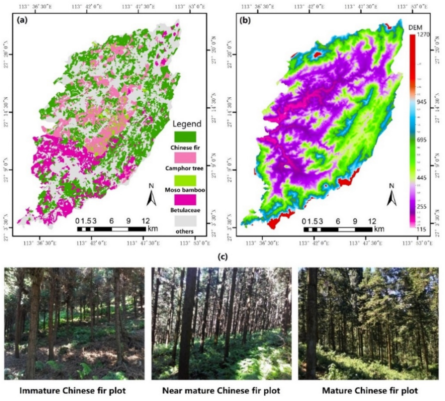
The study site, the Huangfengqiao experimental forest farm, is located in the southeast of Hunan Province, China (Figure 1), and covers an approximate area of 10,122.6 ha. It is influenced by the subtropical monsoon humid climate, with an average annual temperature of 17.8 °C, annual precipitation of 1410.8 mm, and annual frost-free period of approximately 292 d. The area has numerous medium to low mountains with elevations varying from 115 to 1270 m and slopes between 20° and 35°. As shown in Figure 2, the main planted forest stand type is Chinese fir and the area has a total stock volume of 0.89 million cubic meters [35].

Figure 1.
Study area location and distribution of field survey sample plots.
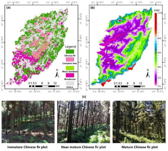
Figure 2.
(a) Distribution of tree species of the study area; (b) the digital elevation model of the study area; (c) photos of Chinese fir in the sample plots.
2.2. Data Preparation
2.2.1. Reference Data
The study area was covered by 50 Chinese fir plantation sample plots measured in the field from 2016 to 2017. The spatial distributions of all the investigated sample plots are shown in Figure 1. The size of each plot was either 20 m × 20 m or 30 m × 30 m, depending upon the topographic features and stem density. The corner and central point positions of the sample plots were measured using a differential global positioning system unit. The basic parameters of all standing trees with a diameter at breast height (DBH) greater than 5 cm were measured in each plot, including DBH, tree height, stem number, crown width, and additional stand information such as topographic factors (e.g., elevation, slope, and aspect) and dominant species. As shown in Formula (1), the GSV of each Chinese fir in the field sample plots was calculated based on the “Table of forest resources survey in Hunan Province” provided by the Hunan forestry department (http://lyj.hunan.gov.cn/, accessed on 16 April 2020). The summary information of the GSV reference data for 50 sample plots is presented in Table 1.
where, D, H is the DBH and height of tree, respectively.

Table 1.
The GSV reference data in the sample plots (m3/ha).
2.2.2. Remote Sensing Data Collection and Pre-Processing
As shown in Table 2, we acquired six GF-2 images of the L1A-level product obtained on December 8, 2016 (http://www.cresda.com/CN/, accessed on 10 May 2019), two ZY-3 images on September 15, 2017 (http://www.cresda.com/CN/, accessed on 10 May 2019), one Sentinel-2 (https://scihub.copernicus.eu/, accessed on 17 March 2019), and Landsat 8 images (http://www.gscloud.cn/, accessed on 15 June 2020) obtained on 14 February 2017, and on 14 April 2017, respectively. The terrain correction of optical images was conducted using digital elevation model (DEM) data with 30 m spatial resolution (http://www.gscloud.cn/, accessed on 15 June 2020), and terrain feature variables at the pixel level, such as slope, aspect, and elevation, were extracted for GSV estimation from the DEM data of the study area. Data from four sensors, with a spatial resolution ranging from 1 m to 30 m, were selected as the optical remote sensing data source for GSV estimation in this study (Table 3). The nearest-neighbor interpolation method was used to resample the selected band images of GF-2, ZY-3, and Sentinel-2 to 30 m in order to unify the image resolution and DEM data so that the pixel size accurately corresponds with the sample plot.
Table 2.
Basic information of four remote sensing image data sources.
Table 3.
Spectral bands of the GF-2, ZY-3, Sentinel-2, and Landsat 8 images used in the study.
3. Methods
3.1. Research Framework
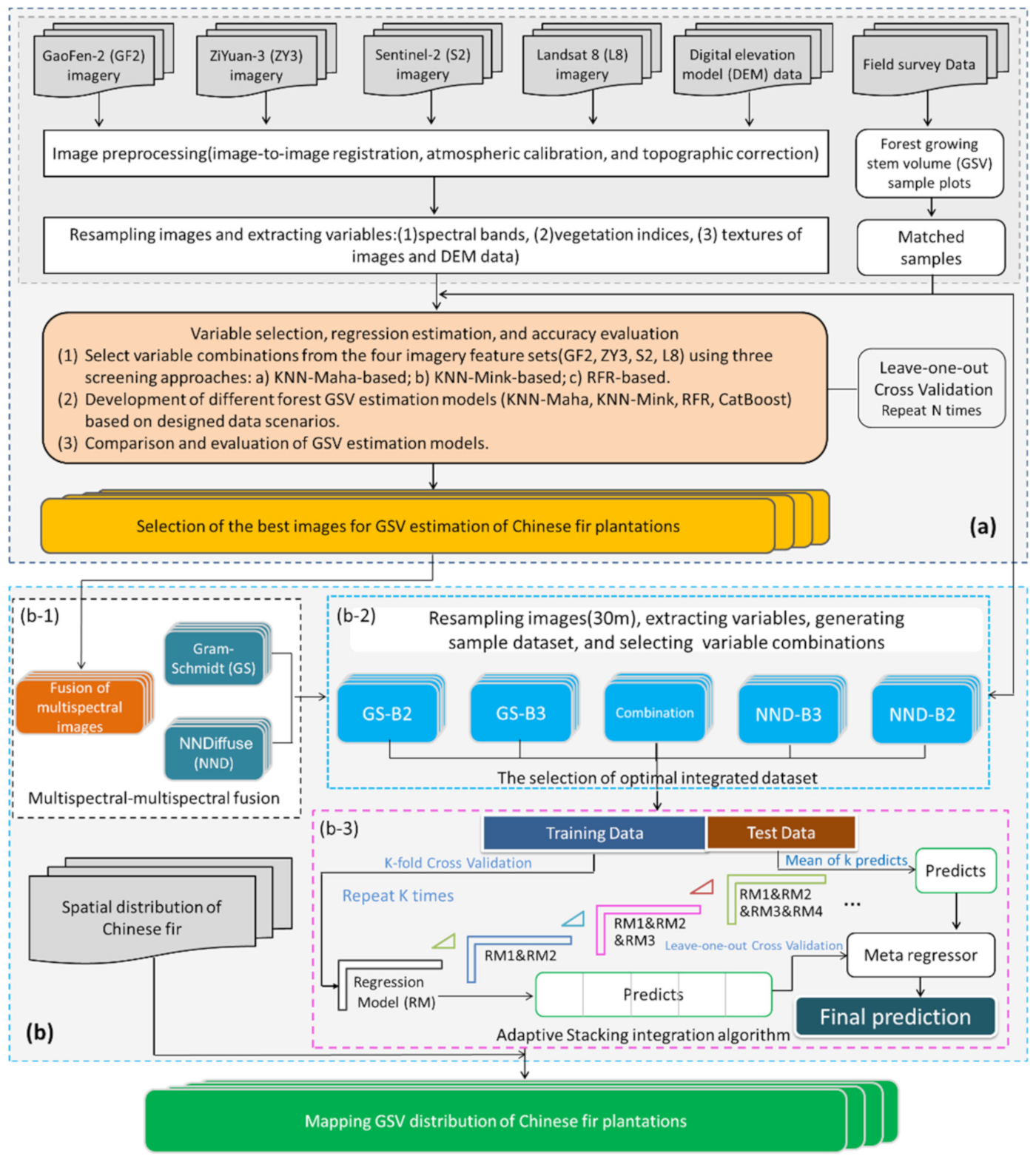
To improve the GSV estimation accuracy of Chinese fir plantations, we examined four optical images datasets and explored the corresponding solutions (Figure 3). The specific content included the following five steps:
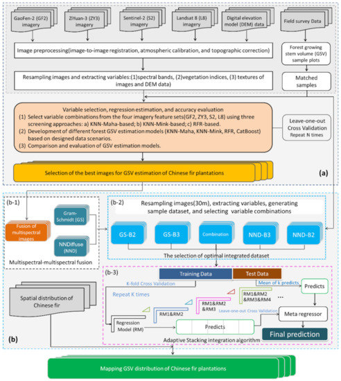
Figure 3.
The research framework for forest GSV estimation based on adaptive-Stacking algorithm. (a) Selection of the most suitable image for GSV estimation; (b) (b-1) Multispectral image fusion, (b-2) selection of optimal integrated dataset, (b-3) flow chart of adaptive stacking ensemble algorithm.
- (1)
- Four remote sensing image datasets were selected (Landsat 8, Sentinel-2, ZY3, GF-2) and vegetation index, texture features, and terrain features were extracted, and combined with the GSV measurement data of the field plots to generate training sample sets.
- (2)
- Three feature combination optimization methods (e.g., KNN-Mink-based, KNN-Maha-based, and RFR-based methods (they are explained in detail in Section 3.3)) were used to select the optimal feature variable combination, subsequently employing KNN-Mink, KNN-Maha, RFR, and Catboost algorithms to build the GSV estimation models, and evaluating GSV estimation accuracy and saturation, and selecting the better medium- and high-resolution images for further GSV estimation research.
- (3)
- The selected medium- and high-resolution multispectral images were fused using Gram-Schmidt (GS) [19] and NND pan sharpening algorithms to obtain a variety of fusion image datasets; the feature combinations were selected subsequent to their extraction, and four regressor algorithms were employed to build the GSV estimation models, from which the best fusion data and corresponding estimation models were selected.
- (4)
- An adaptive-stacking ensemble algorithm that implements the iterative selection of basic regressors and the automatic optimization of hyperparameters for modeling the GSV was employed, and the GSV estimation performance of the adaptive-stacking ensemble model was explored based on the best fusion data.
- (5)
- The GSV distribution of the study area was predicted and mapped based on the best data scheme obtained and the GSV estimation model.
3.2. Feature Variable Extraction Based on Image Data
As shown in Table 4, we extracted four categories of feature variables from GF-2, ZY-3, Sentinel-2, Landsat 8, and DEM images, including spectral information, vegetation indices, texture features, and terrain factors. The spectral information is the pixel spectral reflectance of the resampled original multispectral image. For sentinel-2, only ten bands with original spatial resolutions of 10 m and 20 m were used in this study. We employed four, four, and seven multispectral bands from the GF-2, ZY-3, and Landsat 8 images, respectively, and calculated four types of vegetation indices widely used in forest parameter prediction [19]. The elements in the gray-level co-occurrence matrix (GLCM) represent the joint distribution of the gray levels of two pixels with a certain spatial position relationship. Thus, the GLCM is a statistical-based texture feature extraction method that is frequently used to extract image texture features, such as the image mean, variance, contrast, homogeneity, entropy, dissimilarity, second moment, and correlation [19]. The elevation, slope, and aspect were extracted as terrain factors from the DEM images. Terrain texture is an important factor for distinguishing different landforms, whose features usually have a certain impact on the growth rate of forests. Thus, there is a theoretical relationship between the terrain-based texture feature variables and forest GSV values. Therefore, this study also extracted terrain texture feature variables from the elevation, slope, and aspect images of the study area.
Table 4.
All feature variables extracted from GF-2, ZY-3, Sentinel-2, and Landsat 8 images in this study. We extracted texture factors from optical images, Elevation, Slope, and Aspect data with the step size (1,1], and the window size (3 × 3, 5 × 5, 7 × 7, 9 × 9).
3.3. Feature Combination Optimization Program Based on Regression Models
Numerous feature variables generate a high calculation load for forest GSV modeling, in addition to increasing the risk of overfitting of the estimation model. Therefore, feature selection is particularly important for the GSV estimation. The feature combination optimization method established by previous studies performs better than the SMLR and RF feature selection methods for forest parameter estimation based on remote sensing technology [19,51,56]. In this study, two KNN algorithms [59,60], including the Minkowski distance KNN (Formula (2)), Mahalanobis distance KNN (Formula (3)), and a regression tree algorithm (RFR) were used as regression models to select the optimal feature combination with the minimum root mean square error (RMSE) between the measured and estimated GSV values. These three feature combination optimization methods are denoted as KNN-Mink-based, KNN-Maha-based, and RFR-based, respectively.
where X is the feature space with an n-dimensional vector, , ∈X; p ≥ 1; is the covariance matrix of the sample dataset, is the inverse matrix of , and T is the matrix transposition.
For each iteration, the feature combination optimization program selects a feature variable from the candidate feature set in turn and adds it to the optimal feature set Best_F, then employs the KNN or RFR algorithm to construct the GSV estimation model, subsequently employing the leave-one-out cross validation (LOOCV) method to calculate the GSV estimation RMSE value. The program determines the best one in the current candidate feature set according to the minimum RMSE principle and when the iteration termination condition is satisfied, the program exits, and the optimal feature variable combination Best_F is obtained.
3.4. Multispectral Image Data Fusion and Combination
In this study, the GSV estimation performance of four optical remote sensing image datasets were compared, two images with the highest GSV saturation and estimation accuracy were identified, and the data integration scheme suitable for GSV estimation was subsequently explored through image data fusion and combination. Remote sensing image data fusion usually adopts the method of fusing high-resolution multi-spectral image with medium-resolution multi-spectral images, in order to obtain a fusion image with both high spatial resolution and rich spectral information similar to medium-resolution images. Furthermore, since each multispectral band of high-resolution images can be fused with medium-resolution images, a variety of fusion schemes based on different image bands and different fusion algorithms can be explored. Therefore, we can obtain multiple image fusion data with large differences in spectral information, which is convenient for further extraction of the feature variables used for GSV estimation, construction of a corresponding GSV estimation model for each data scene based on the selected features, and exploration of the most suitable remote sensing image fusion data for GSV estimation.
To find a multi-spectral image fusion method suitable for forest AGB estimation, we compared two classic fusion algorithms, GS and NND. In this study, each of the two multispectral bands (B2_green and B3_red) of the high-resolution image (GF-2 or ZY-3) was fused with the medium-resolution image (Sentinel-2 or Landsat 8). The fused images are denoted by the fusion method and the band names. For example, the image obtained after fusion of the B2_green image with Sentinel-2 or Landsat 8, using the NND method, is denoted as NND_B2. For comparison with fusion images, we also examined the combination scheme of images, which integrated all feature variables of the two images as a single sample dataset.
3.5. Forest GSV Estimation Modeling Based on Adaptive-Stacking Ensemble Algorithm
This study aims to address the disadvantages of underestimation and overestimation in the estimation results of a single model, and plans to adopt the stacking machine learning model ensemble algorithm that integrates the prediction results of the basic regression models as independent variables of a meta-regressor for secondary prediction. However, the selection of the base-and meta-models and hyperparameter optimization are the keys to the stacking integration algorithm. Therefore, based on the analysis of different model architectures and estimation performance, this study comprehensively considers the coupling mechanism between the models and realizes the adaptive integration of the stacking model through the iterative selection of models and the automatic optimization of hyperparameters. As shown in Figure 3, the adaptive stacking ensemble learning algorithm flow is as follows:
Step 1: The training dataset is inputted, and the base regression model (RM 1), RM i, Meta Regressor, Best_RMSE, and other related parameters are initialized.
Step 2: Using the LOOCV method, one out of all samples will be set aside as the test sample (TestData), and the other samples are input into the training dataset as training samples (TrainData). The training dataset is also divided into K parts. Each time, the predictions are made simultaneously in one part of TrainData and TrainData as a whole., K prediction results are thus obtained after K iterations.
Step 3: By comparing the RMSE loop traversal optimization model parameters, the K prediction results of models RM 1 and RM i in step 1 are used as the new training data set feature variables F1 and F2, and the K test samples of RM 1 and RM i are used to predict the results. The average values are used as feature variables V1 and V2 of the new test sample, respectively.
Step 4: The set of F1, F2, and the set of V1 and V2 are used as the training sample set and test sample set of the meta-regressor, respectively, and the meta-regressor is used to fit the training sample and build the regression model, and make predictions on the test samples to obtain the prediction results.
Step 5: On comparing the RMSE of the model cross-validation results, if the conditional discriminant best_RMSE < Best_RMSE is satisfied, integration of the new basic regression model RM I is continued, the relevant parameters of the existing integrated model are updated, subsequently returning to Step 2; if the conditions are not met, the loop is exited, the optimal integrated model is outputted and the final prediction result is obtained.
Considering the superior performance of the KNN, RFR, and CatBoost algorithms in forest parameter estimation, this study used the feature variable selected by the KNN-based or RFR-based feature combination optimization program to construct various forest GSV estimation models, including the Minkowski distance KNN (KNN-Mink), Mahalanobis distance KNN (KNN-Maha), RFR, and CatBoost algorithms. Additionally, these models are used as basic regression models to further develop the AdaStacking ensemble model, and automatically screen and optimize basic regressors and hyperparameters through iterative procedures.
3.6. Model Evaluation and Saturation Calculation
To maximize the use of the existing field observation sample dataset, the performance of the GSV estimation model was examined in this study, using the LOOCV method. In each iteration, one sample was selected as the test sample, and the remaining 49 samples were used to establish the GSV estimation model based on the regression algorithm. The GSV estimation values of all the samples were obtained after 50 looped repetitions. By comparing the estimated GSV value obtained by the GSV estimation model with the observed GSV value measured at the field site, we can obtain the GSV estimation saturation value of each modeling scheme, which is constituted by an image data scene and estimation model. The evaluation indices for various estimation models were calculated based on the estimated and observed GSV values, including the coefficient of determination (R2), RMSE, relative RMSE (RMSEr), and mean absolute error (MAE).
where n is the sample size, is the observed reference GSV value, is the mean of all , is the estimated GSV value from the regression model.
Generally, smaller RMSE, RMSEr, and MAE values indicate a higher accuracy of the estimation model; the larger the R2 value, the better the fit of the model, and the higher the degree of explanation of independent variables with respect to dependent variables.
4. Results and Discussion
4.1. Evaluation of GSV Estimation Performance of Four Image Data Sets
4.1.1. Selection of the Best Predictive Feature Variable Combination of GF-2, ZY-3, Sentinel-2, and Landsat 8 Images
In this study, three feature combination optimization methods, i.e., KNN-Mink-based, KNN-Maha-based, and RFR-based, were used to select feature variables from the GF-2, ZY-3, Sentinel-2, and Landsat 8 image datasets (Table A1). Of the 12 feature variable combinations—composed of four image data scenes and three feature selection methods—66 feature variables were selected, of which 54 were texture feature variables, 11 were vegetation index variables, and 1 was green band spectral information. The most frequently selected texture factors are the second moment, homogeneity, correlation, mean, and entropy, and the selected times were 10, 9, 9, 8, and 6, respectively. In summary, the feature variables selected in this study based on the feature combination optimization program were consistent with the research results of Jiang et al. [41] in forest GSV estimation and Han et al. [60] in forest AGB modeling.
For high-resolution images (GF-2 and ZY-3), due to the lack of red edges and short-wave infrared bands suitable for vegetation growth monitoring, resulting in the vegetation index variables being insufficiently sensitive to changes in forest GSV [47,48,61]. For medium spatial resolution images (Sentinel-2 and Landsat 8), the selected vegetation index variables increased significantly, especially with the Sentinel-2 image dataset containing three red-edge bands and two short-wave infrared bands. Two methods selected four vegetation index variables each, and the third selected one. Among them, six were related to the red edge band of the Sentinel-2 image, indicating that the red edge bands and short-wave infrared bands of the medium spatial resolution image play an important role in GSV estimation.
4.1.2. GSV Prediction Performance of GF-2, ZY-3, Sentinel-2, and Landsat 8 Images
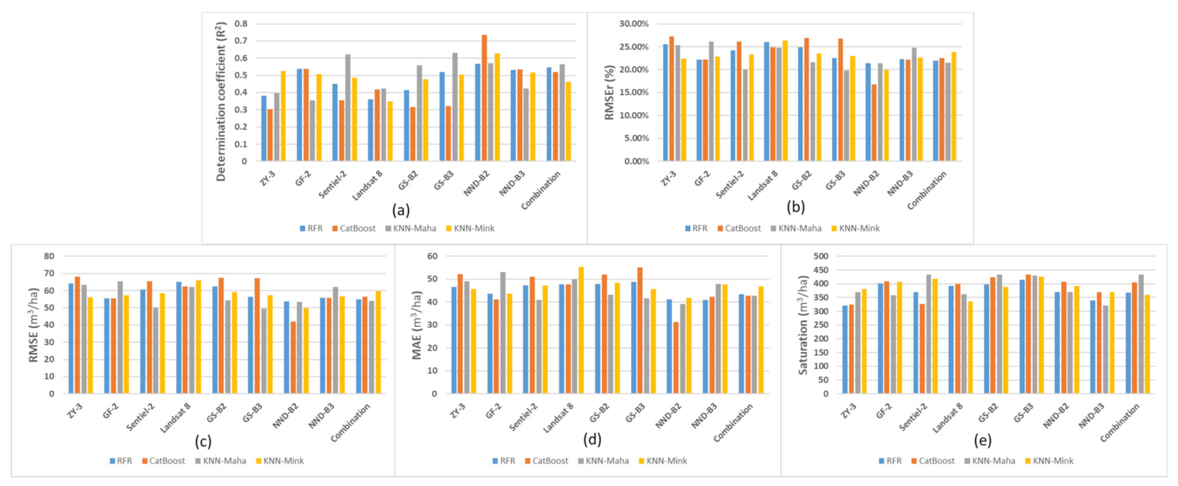
As shown in Figure 4, Figure A1 and Figure A2, the Sentinel-2 and GF-2 image datasets showed the best GSV estimation performance, and their GSV estimated saturation value reached 434 m3/ha and 409 m3/ha, respectively. When using sentinel-2 and GF-2 image data sets to build the GSV estimation model based on four regression algorithms, the minimum RMSEr values were 20.06% and 22.16%, and average RMSEr values of 23.43% and 23.34%, respectively.
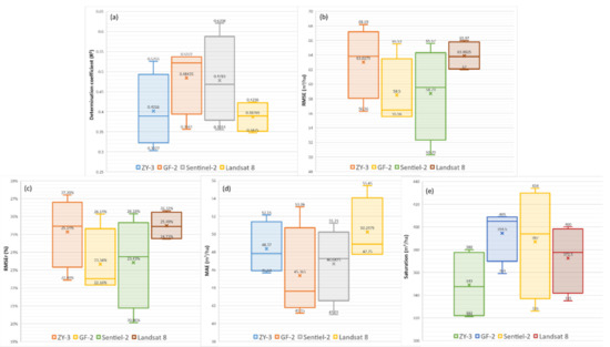
Figure 4.
Based on ZY-3, GF-2, sentinel-2 and Landsat 8 data scenarios, the box plot of various evaluation indexes of GSV estimation results obtained by RFR, CatBoost, KNN-Maha and KNN-Mink modeling algorithms respectively. (a–e) are the R2, RMSE, RMSEr, MAE, Saturation, respectively.
For the GF-2 image dataset, both the RFR and CatBoost models exhibit good GSV estimation performance. When the GSV value is large, there is no underestimation that the absolute deviation is 50% greater than the average value of GSV samples; however, when the GSV value is less than 150 m3/ha, the overestimation is evident. The GSV estimation performance of the ZY-3 image dataset was inferior to that of the GF-2 image. The underestimation of high GSV value areas is particularly severe, resulting in the GSV estimated saturation value of the ZY-3 image being much lower than that of the other three images. For the Sentinel-2 image data set, the GSV estimation performance of the KNN-Maha model performed the best, exhibiting the lowest estimated MAE and RMSE values of 41.01 m3/ha and 50.29 m3/ha, respectively. Furthermore, the highest value of the GSV estimated saturation of the Sentinel-2 image is much larger than that of the other three image datasets. The GSV estimation performance of the Landsat 8 image dataset was inferior to that of the other three images. The distribution of GSV estimation residual values shows a highly recognizable linear trend, indicating that the overestimation in the GSV low-value area and the underestimation in the GSV high-value area are both relatively severe.
Astola et al. examined the GSV estimation performance of Sentinel-2 and Landsat 8 images in a boreal forest in Southern Finland and found that the estimation accuracy of Sentinel-2 was higher than that of Landsat 8 images. Their conclusions are consistent with the results of this study. Moreover, the predictive ability of Sentinel-2 VRE images has been reported in recent forest GSV studies [41], tree species classification [59], wetland mapping [58], and biophysical variable prediction [6]. Chrysafis et al. [4] examined the importance of feature variables using the random forest method for GSV estimation and found that SWIR 1 was the most important band for both Sentinel-2 and Landsat 8 images. Our study found that, compared with feature importance analysis, identifying the best combination of feature variables matching with a specific regression model is the key to accurately estimating GSV. For instance, the combination of feature variables selected using the three methods based on the Sentinel-2 dataset is different from the corresponding GSV estimation accuracy. However, all three methods choose the combination of feature variables related to VRE bands and elevation data, indicating that these two parameters play a vital role in GSV estimation.
4.2. GSV Estimation Performance Improvement Method Based on Multi-Spectral Image Fusion
Although the GSV estimation performance of GF-2 and Sentinel-2 images is higher than that of ZY-3 and Landsat 8, problems still persisted. For example, GF-2 images maintained a certain overestimation in low GSV value areas, and Sentinel-2 images exhibited a large estimation deviation in the GSV value range of 200 m3/ha–400 m3/ha, indicating clear underestimation. To further improve the accuracy of GSV estimation, GS and NND methods were used to perform multispectral image fusion on GF-2 and Sentinel-2, which generated four fusions: GS-B2, GS-B3, NND-B2, and NND-B3 image data scenes. This study used three feature variable combination optimization methods to screen feature variables based on one combination data scene and four fusion datasets of GF-2 and Sentinel-2, and utilized four regression algorithms to establish the GSV estimation models.
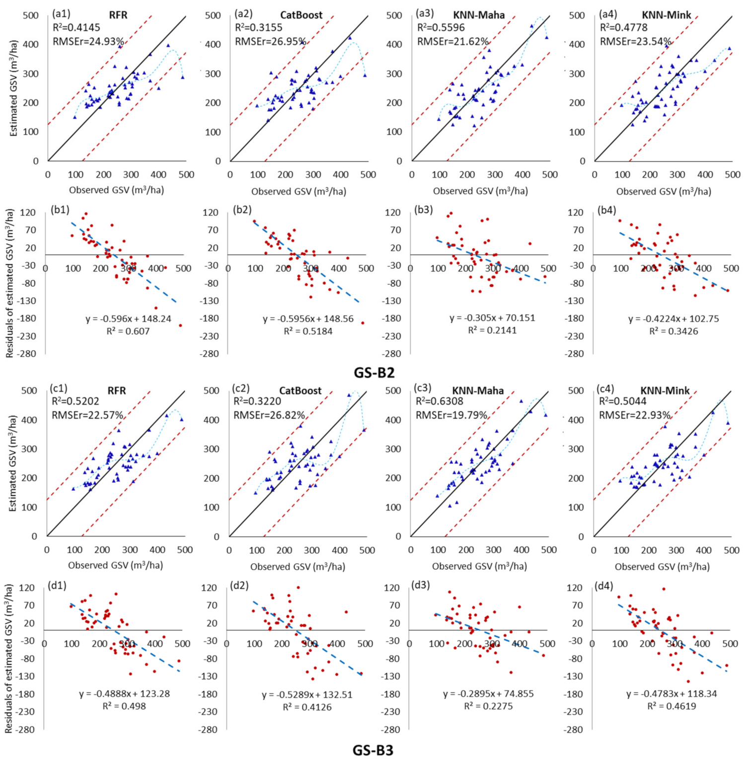
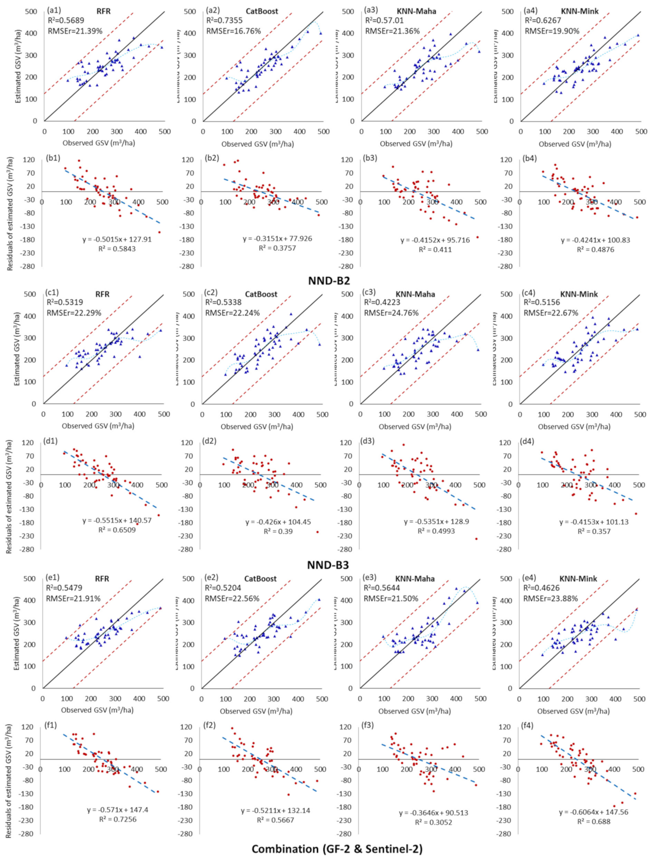
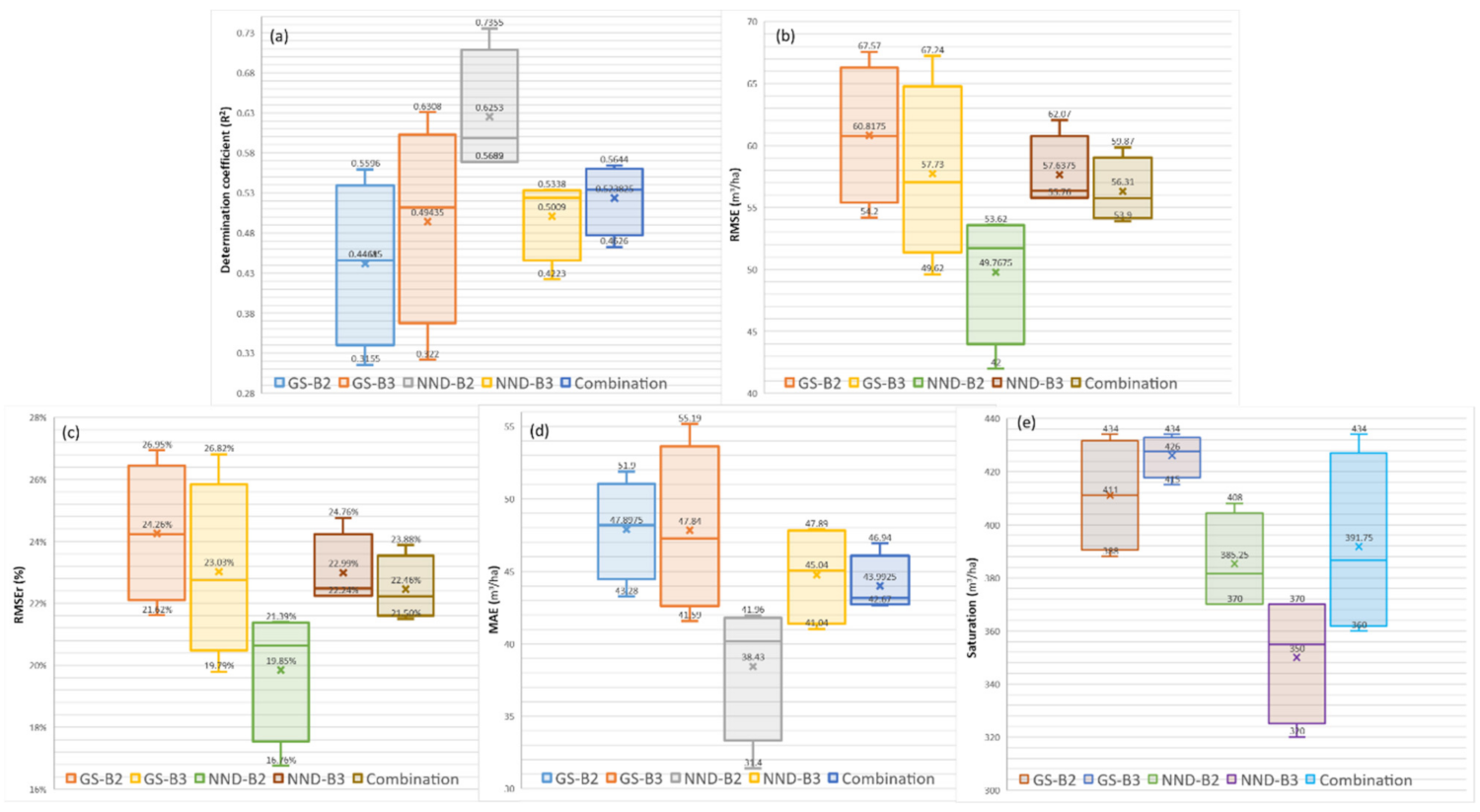
As depicted in Figure 5, Figure 6, Figure 7 and Figure 8, for five image data scenarios, including the combination dataset of GF-2 and Sentinel-2, and four fusion images, the GS-B3 and NND-B2 datasets have the best GSV estimation performance, with the minimum GSV estimation RMSEr values of 19.79% and 16.76%, respectively. Compared with the GSV estimation results of the GF-2 and Sentinel-2 image data scenarios, the optimal estimation R2 of NND_B2 was 36.9% and 18.5% higher than those of the GF-2 and Sentinel-2, and the best RMSE value was 24.4% and 16.5% lower, respectively. As seen from the scatter plot of Figure 6(e2), when the CatBoost model was employed, the estimation GSV based on the NND-B2 dataset had a highly concentrated distribution and clear fitting trend, with no evident overestimation or underestimation. Moreover, all four GSV estimation models based on the NND-B2 image dataset have competent estimation accuracies; the average value of the GSV estimation RMSEr is 19.85%, which is significantly lower than those of the original image and fusion image datasets. Li et al. [19] employed the fusion data of GF2 and Landsat 8 multispectral images to estimate the GSV of Chinese pine and larch plantations in northern China. Interestingly, they found GF2 red to be the most suitable band for fusion with Landsat 8 multispectral images in the GSV estimation process. In this study, when the GS method was used to fuse two multispectral images, the GF-2 red band exhibited an appreciable performance, and the GS-B3 image obtained a satisfactory estimation accuracy; however, when the NND fusion method was employed, the fusion image NND-B2 obtained by the GF-2 green band had the highest estimated performance. The different climate, tree species, and terrain with respect to our study could explain the differences in the results.
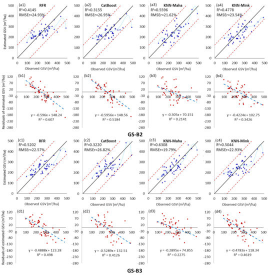
Figure 5.
Scatter plot and residual distribution of the predicted GSV results obtained by the RFR, CatBoost, KNN-Maha, and KNN-Mink modeling algorithms under the fused images of GS-B2 (a1–b4) and GS-B3 (c1–d4) dataset scenarios. The blue dotted line is the fitting trend of the sixth-order polynomial between the estimated value and the observed value of GSV.
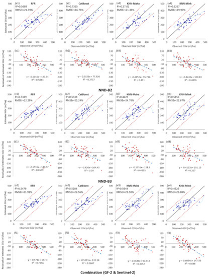
Figure 6.
Scatter plot and residual distribution of the predicted GSV results obtained by the RFR, CatBoost, KNN-Maha, and KNN-Mink modeling algorithms under the fused images of NND-B2 (a1–b4) and NND-B3 (c1–d4), and the combined (e1–f4) of GF-2 & Sentinel-2 dataset scenarios. The blue dotted line is the fitting trend of the sixth-order polynomial between the estimated value and the observed value of GSV.
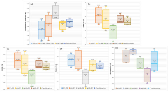
Figure 7.
Based on the fused and the combined GF-2 and Sentinel-2 dataset scenarios, the box plot of various evaluation indexes of GSV estimation results obtained by RFR, CatBoost, KNN-Maha and KNN-Mink modeling algorithms, respectively. (a–e) are the R2, RMSE, RMSEr, MAE, and Saturation, respectively.
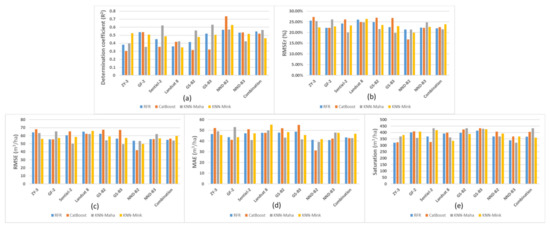
Figure 8.
Comparison of various evaluation indexes of GSV estimation results based on nine dataset scenarios obtained by RFR, CatBoost, KNN-Maha and KNN-Mink modeling algorithms, respectively. (a–e) are the R2, RMSEr, RMSE, MAE, and Saturation, respectively.
4.3. GSV Estimation Ability of the AdaStacking Ensemble Model
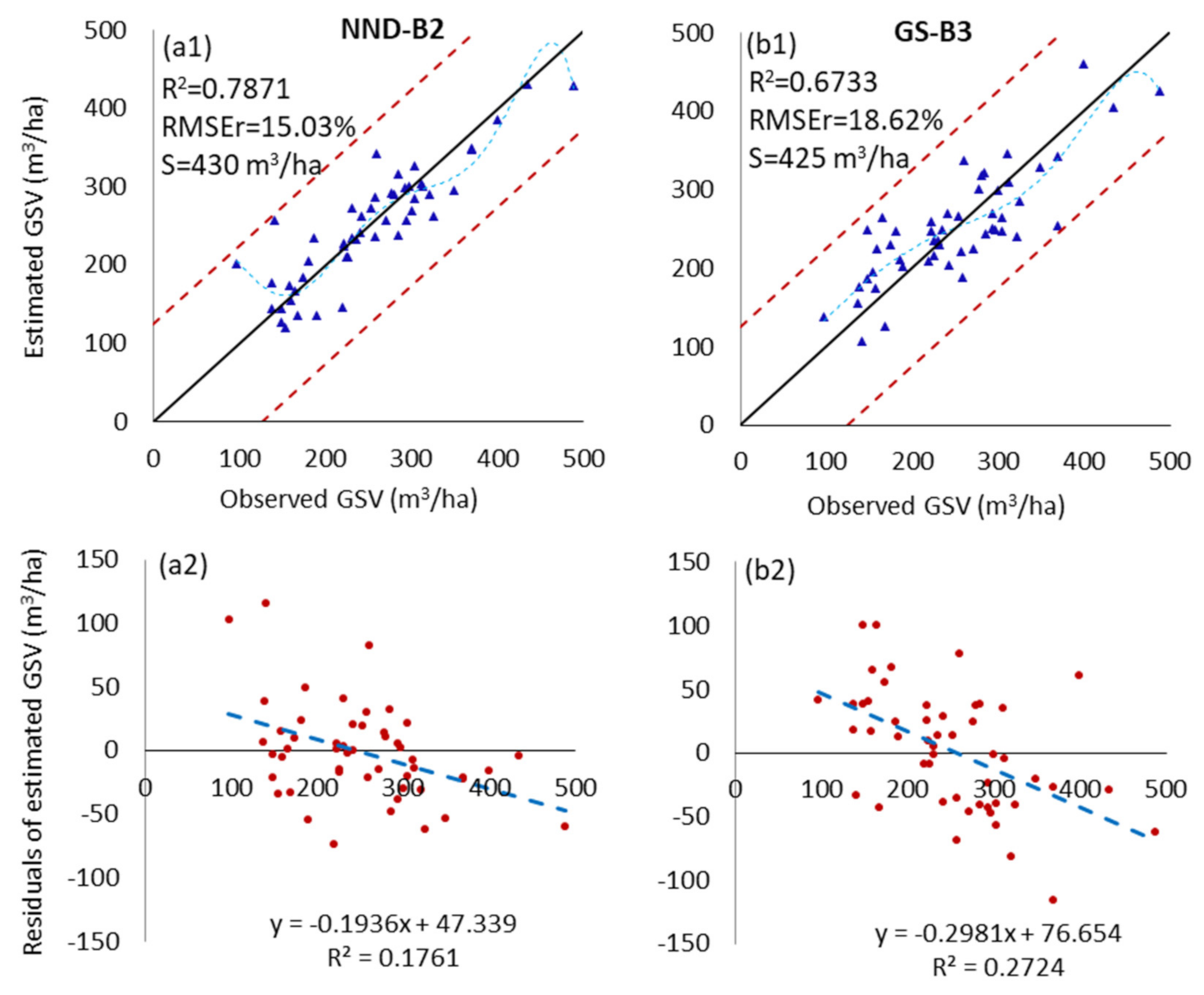
The GSV estimation performance for the GS-B3 fusion image dataset was only marginally higher than that of the Sentinel-2 image. When the GSV value exceeded 300 m3/ha, the underestimation issue was particularly serious. Although the estimation accuracy of NND-B2 is greatly improved compared to that of GF-2 and Sentinel-2, the estimated saturation of GSV is lower than that of Sentinel-2. To further explore the possibility of improving the GSV estimation performance, the AdaStacking ensemble model was developed based on the GS-B3 and NND-B2 image datasets and their corresponding optimal feature combinations. As shown in Figure 9, by applying the AdaStacking model ensemble method, the estimation performance of the NND-B2 and GS-B3 images is further improved. The best obtained estimation RMSEr was 25.1% and 7.2%, respectively, lower than that of Sentinel-2. Specifically, the adaptive ensemble of estimation models has alleviated the underestimation problem of the high-value range of the GSV. The saturation of the GSV estimation value of the AdaStacking model based on NND-B2 was 5.4% higher than that of the KNN-Maha model.
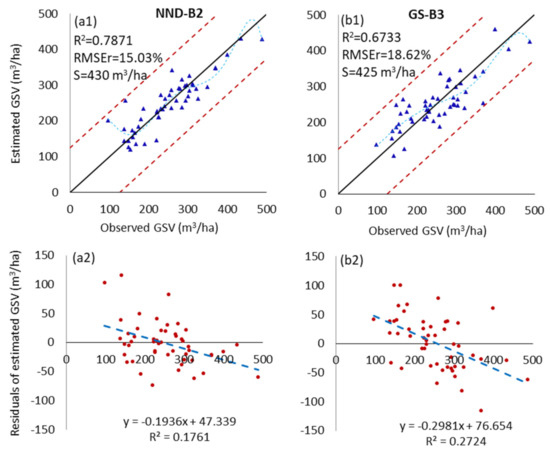
Figure 9.
Scatter plots of the observed and estimated GSV values (m3/ha) using the NND-B2 and GS-B3 datasets with feature variables selected by the RFR-based method. (a1,a2), the GSV estimated from the fused image NND-B2 using the AdaStacking model. (b1,b2), the GSV estimated from the fused image GS-B3 using the AdaStacking model.
Wang et al. [62] predicted the forest unit GSV based on the reference data provided by the National Forestry Science Data Sharing Service Platform in China, and found that the best unit GSV estimation accuracy of the single model was 83.81%, and the multi-model estimation by the stacking ensemble was 84.55%. Although they used the Pearson correlation coefficient and the least absolute shrinkage and selection operator (LASSO) regression method to filter and select features, and employed the stacking ensemble method to integrate various regression models, the GSV estimation performance was not ideal; in particular, the stacking ensemble method was only 0.88% more efficient than the single model. The possible reason for this is that their feature selection method does not consider the heterogeneity between the feature variables and the combination effect relationship, and does not use texture feature factors reflecting forest resource space distribution details. Most importantly, the data source was not selected based on the spectral saturation of remote sensing images, and there is no multispectral fusion processing on the image. Moreover, Jiang et al. [41] estimated coniferous plantation GSV based on Sentinel-2 images using the SRF method and RFR model in North China, and found that the GSV estimation RMSEr minimum was 28%. Their accuracy was significantly lower than that of the AdaStacking method proposed in this study, where the GSV estimation minimum RMSEr value reached 15.03% and the maximum R2 value was 0.7871 with the AdaStacking model based on the NND-B2 image.
4.4. Predicting and Mapping the GSV of Coniferous Plantation
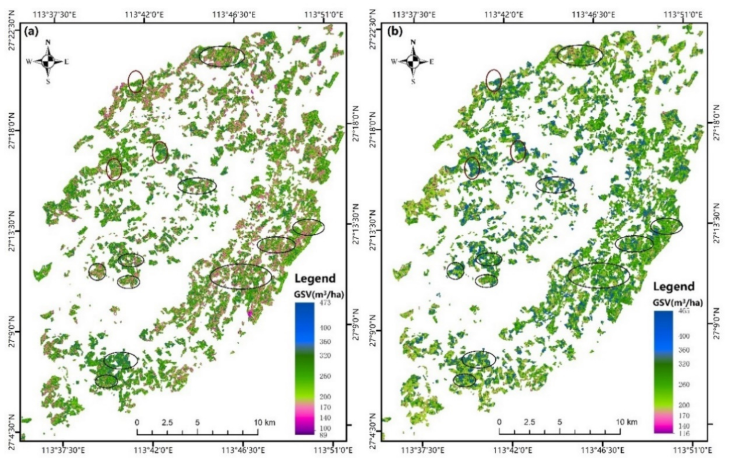
We mapped the spatial GSV distribution of Chinese fir plantations in the study area, using the AdaStacking model based on the fused images GS-B3 and NND-B2. Figure 10a,b depict the estimated GSV distribution map obtained from the NND-B2 and GS-B3 datasets, respectively. Figure 10a exhibits additional rose red and light green pixels and fewer dark green and blue areas than Figure 10b, especially in the east and south of the study area. Figure 9 shows that when the AdaStacking model is implemented, the overestimation problem of GS-B3 is significantly more severe than that of NND-B2 in the low GSV range of 150–200 m3/ha, exhibiting an overestimation problem even the GSV value exceeding 300 m3/ha. This could potentially be due to the working mechanism of the basic KNN-Maha model used in the AdaStacking model integration and the complexity of the forest ecosystem. The estimation accuracy of the KNN algorithm based on the distance measurement mechanism is mainly determined by the number of nearest neighbors selected. When the number is too large, the estimated result tends closer to the sample mean. When the number of neighbors is too small, the estimation model is prone to overfitting. Typically, to ensure the total estimation accuracy, the value of the number of neighbors (n_neighbors) is not set very high. In the forest ecological environment with large spatial heterogeneity, due to the influence of canopy shadow, slope, aspect, and sunlight angle, even forests with very different GSV values may produce imagery with analogous spectral information. Therefore, when the proportion of samples with a higher GSV value in the training sample set is larger and the n_neighbors of the KNN model is smaller, overestimation is highly likely.

Figure 10.
(a) and (b) are the GSV distribution maps of Chinese fir Plantations in the study area estimated by AFCO-RFR method and AdaStacking model from the fusion images NND-B2 and GS-B3, respectively.
4.5. Uncertainty Analysis of Forest GSV Estimation
The forest GSV estimation accuracy based on remote sensing technology is influenced by various factors, including the optical remote sensing image prediction ability, field measurement error, selection of predictive characteristic variables, generalization ability of modeling methods, and differences in physiological characteristics between tree species [24,25].
First, the differences in the spatial and spectral resolution of images taken by different optical sensors will lead to differences in the perception and sensitivity of forest vegetation spectral information. This study’s results show that Sentinel-2 images with multiple VRE bands have significantly higher GSV estimation accuracy and saturation than Landsat 8 images with 30 m resolution, and that GF-2 with 1 m resolution has better GSV estimation performance than ZY-3, thus elucidating the necessity of selecting a suitable remote sensing image data source for accurate GSV estimation. Second, the errors in the measured data of the forest survey sample plot will also have an impact on the GSV modeling accuracy. The GSV sample data collection time span of this study was approximately one year. During this period, the growth of the forest could also generate an error in the observed GSV value. Third, the extraction and selection methods of predictive feature variables directly affect the accuracy and saturation of the model. For example, when employing RFR-based, KNN-Maha-based, and KNN-Mink-based methods to select feature variable combinations of Sentinel-2 images, the estimated GSV saturation values were 370 m3/ha, 434 m3/ha, and 418 m3/ha, respectively. Fourth, variations were observed in the model generalization performance and estimation accuracy of the different modeling algorithms. For example, the feature variables of RFR and CatBoost algorithms for modeling were identical; however, in most data scenarios, especially for the NND-B2 dataset, their estimation performance had certain variances, and the estimated RMSEr value obtained by the CatBoost algorithm was 21.6% lower than that of the RFR algorithm. Finally, differences in canopy structure and spectral reflectance characteristics between the tree species led to differences in the GSV models and the estimation results, causing classification errors of forest tree species to affect the estimation accuracy of GSV. In summary, the study considers that the above five factors will produce significant uncertainty in the forest GSV remote sensing estimation results and in the estimation of other forest parameters.
5. Conclusions
In this study, GSV estimation performance of four optical remote sensing images with different spatial resolutions and spectral resolutions for the Chinese fir plantations was examined. Three feature combination optimization methods and four regression algorithms were utilized to select features and to develop the GSV estimation models, obtain and assess four multispectral fusion image datasets, and propose an AdaStacking ensemble algorithm for modeling the GSV. The results indicated that: (1) the texture feature variables extracted from multispectral imagery and DEM data were highly correlated with the observed GSV samples. Texture features accounted for 81.82% of all the feature variables selected by the three feature combination optimization methods, and (2) the obtained GSV estimation minimum RMSE based on four image datasets (GF-2, ZY-3, Sentinel-2, and Landsat 8) were 22.16%, 22.44%, 20.06%, and 24.73%, respectively. The GSV estimation saturations of the four image datasets were 409 m3/ha, 380 m3/ha, 434 m3/ha, and 400 m3/ha, respectively. It was observed that Sentinel-2 had the highest estimation accuracy and saturation among the four image datasets, followed by GF-2, and (3) the new image data obtained by fusing multi-spectral images of different spectral and spatial resolutions effectively coupled the advantages of the two images and significantly improved the GSV estimation performance. Among the four fusion images obtained by GF-2 and Sentinel-2 using GS and NND methods, the NND-B2 image exhibited the best estimation accuracy with an estimated optimal RMSE that was 24.4% and 16.5% lower than GF-2 and Sentinel-2, respectively; and (4) the AdaStacking algorithm proposed in this study adaptively selected the basic regression model and realized the automatic optimization of model hyperparameters through an iterative procedure, exhibiting better GSV estimation performance than a single model. This study examined the data saturation issue of four optical remote sensing image datasets in coniferous plantations and explored a novel approach to improve GSV prediction performance. Our research provides some new insight into the application of optical imagery and advanced remote Sensing algorithms for estimating the GSV of coniferous plantations.
Author Contributions
Conceptualization, X.L.; methodology, X.L.; software, X.L.; validation, X.L., Z.L.; formal analysis, X.L., M.Z. and H.L.; investigation, X.L., J.L., M.Z., Z.L. and H.L.; resources, X.L., J.L., Z.L.; data processing, X.L., J.L., Z.L.; original draft, X.L.; review and revision, X.L., H.L.; final editing: X.L.; visualization, X.L.; supervision, H.L., J.L.; project administration, X.L., J.L.; funding acquisition, X.L., H.L. All authors have read and agreed to the published version of the manuscript.
Funding
This study was financially supported by National Key R&D Program of China project “Research of Key Technologies for Monitoring Forest Plantation Resources” (N#:2017YFD0600900); National Natural Science Foundation of China (N#:41901385); Hunan Provincial Innovation Foundation For Postgraduate (N#: CX20200694).
Institutional Review Board Statement
Not applicable.
Informed Consent Statement
Not applicable.
Data Availability Statement
The observed GSV data from the sample plots and spatial distribution data of forest resources presented in this study are available on request from the corresponding author. Those data are not publicly available due to privacy and confidentiality. The Sentinel-2 images of the L1-level product were obtained from Copernicus data center website at https://scihub.copernicus.eu/ (accessed on 17 March 2020). The GF-2 and ZY-3 images are available from China Centre for Resources Satellite Data and Application website at http://www.cresda.com/CN/ (accessed on 10 May 2020). The Landsat 8 images and DEM data were downloaded from geospatial data cloud (http://www.gscloud.cn/ (accessed on 15 June 2020)).
Conflicts of Interest
The authors declare no conflict of interest.
Appendix A
Table A1.
Selected feature variables from the GF-2, ZY-3, Sentinel-2 (S2), and Landsat 8 (L8) images dataset by three feature combination optimization methods, including KNN-Mink-based, KNN-Maha-based, and RFR-based. W, Texture window size (3 × 3, 5 × 5, 7 × 7, 9 × 9); Mean, GLCM-mean; Var, GLCM-variance; Hom, GLCM-homogeneity; Con, GLCM-contrast; Dis, GLCM-dissimilarity; Ent, GLCM-entropy; Sec, GLCM-second moment; Cor, GLCM-correlation. For example, GF2_Red_W3_Hom is expressed as a texture feature with the texture window size 3 × 3, homogeneity, that is derived from the GF-2 Red band image.
| Image Dataset | Feature Selection Method | Selected Feature Variables |
|---|---|---|
| GF-2 | KNN-Mink-based | GF2_Red_W3_Hom GF2_NIR_W7_Hom GF2_Red_W5_Hom GF2_Red_W3_Sec |
| KNN-Maha-based | GF2_Red_W3_Hom GF2_Blue_W3_Var | |
| RFR-based | GF2_Red_W3_Hom Elevation_W3_Ent Slope_W5_Sec | |
| ZY-3 | KNN-Mink-based | ZY3_Blue_W5_Mean ZY3_Blue_W9_Cor ZY3_ Red_W5_Cor ZY3_ Blue_W3_Hom Elevation_W3_Sec ZY3_ Blue_W7_Mean |
| KNN-Maha-based | ZY3_NIR_W7_Var ZY3_ Blue_W5_Cor ZY3_Green_W3_Con ZY3_ Blue_W5_Sec ZY3_Green | |
| RFR-based | ZY3_Red_W7_Mean ZY3_NIR_W7_Con Elevation_W3_Sec Slope_W3_Hom Slope_W3_Ent Slope_W3_Cor Elevation_W7_Cor | |
| Sentinel-2 | KNN-Mink-based | S2_VRE3_W9_Sec Elevation_W3_Sec S2_RVI6_8 S2_NDVI9_10 S2_VRE3_W5_Sec S2_NDVI1_2 S2_RVI6_7 |
| KNN-Maha-based | S2_Green_W5_Ent Elevation_W3_Ent S2_NDVI1_2 S2_DVI1_8 S2_Red_W5_Mean S2_DVI2_6 S2_RVI1_5 S2_NIR_W9_Var Elevation_W5_Con Slope_W7_Cor | |
| RFR-based | Elevation_W3_Ent S2_Red_W5_Var Slope_W5_Cor S2_DVI3_4 | |
| Landsat 8 | KNN-Mink-based | L8_NDVI5_6_3 L8_Red_W3_Dis L8_SWIR2_W9_Dis Slope_W3_Ent Slope_W3_Hom Slope_W7_SecElevation_W5_Hom |
| KNN-Maha-based | L8_NDVI5_6_3 L8_ Red_W3_Con L8_Coast_W7_Mean L8_Coast_W3_Cor L8_Red_W3_Ent L8_SWIR2_W7_ Mean L8_SWIR2_W9_Con L8_SWIR1_W5_Sec | |
| RFR-based | L8_Red_W3_Cor L8_Blue_W5_Mean L8_ Blue_W3_Mean |
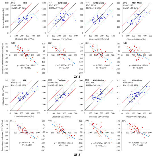
Figure A1.
Scatter plot and residual distribution of the predicted GSV results obtained by the RFR, CatBoost, KNN-Maha, and KNN-Mink modeling algorithms under the ZY-3 (a1–b4) and GF-2 (c1–d4) dataset scenarios. The blue dotted line is the fitting trend of the sixth-order polynomial between the estimated value and the observed value of GSV.
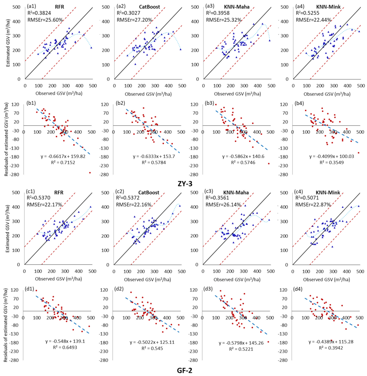
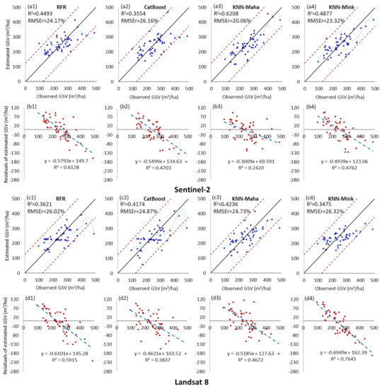
Figure A2.
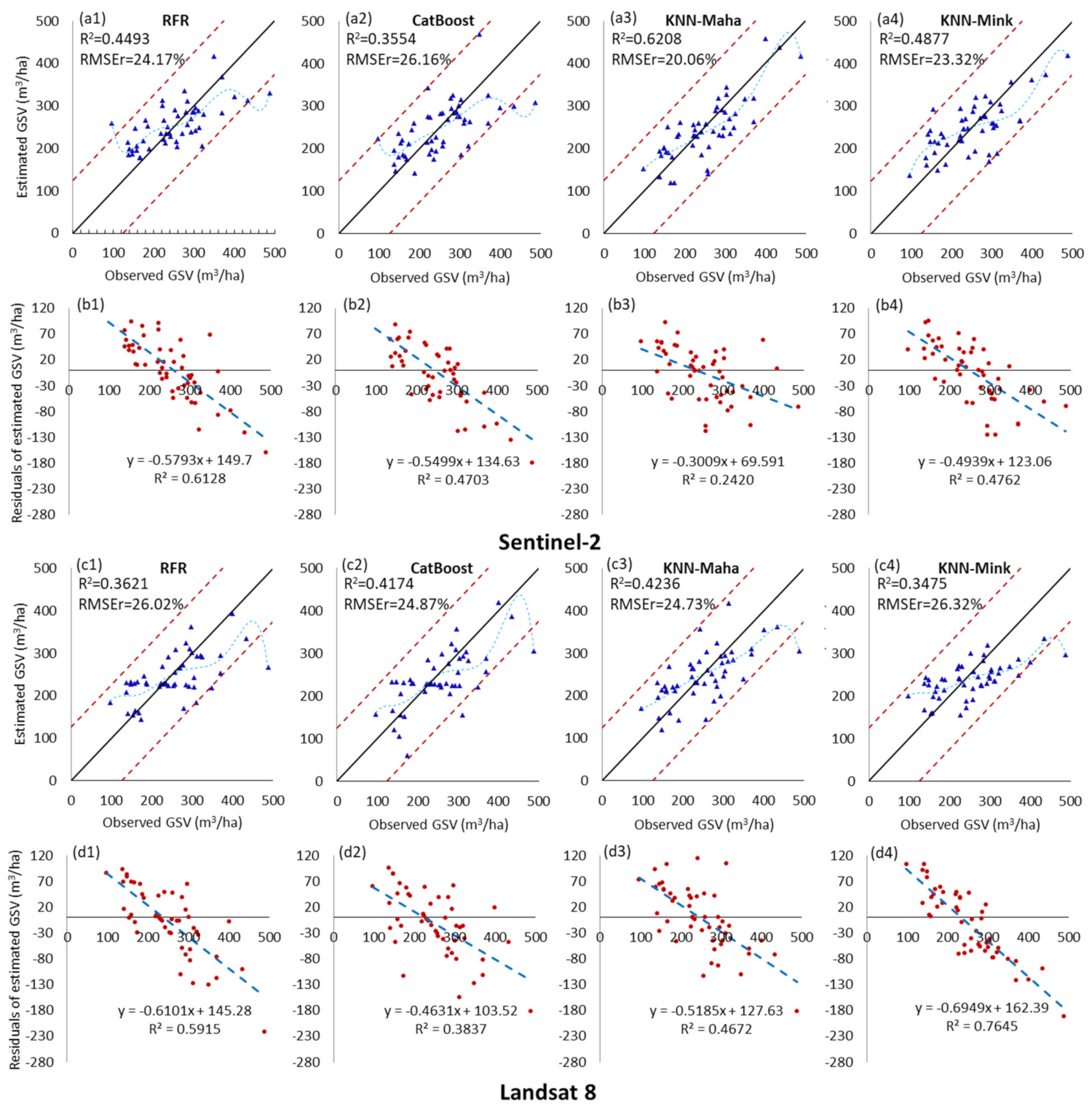
Scatter plot and residual distribution of the predicted GSV results obtained by the RFR, CatBoost, KNN-Maha, and KNN-Mink modeling algorithms under the Sentinel-2 (a1–b4) and Landsat 8 (c1–d4) dataset scenarios. The blue dotted line is the fitting trend of the sixth-order polynomial between the estimated value and the observed value of GSV.
Figure A2.
Scatter plot and residual distribution of the predicted GSV results obtained by the RFR, CatBoost, KNN-Maha, and KNN-Mink modeling algorithms under the Sentinel-2 (a1–b4) and Landsat 8 (c1–d4) dataset scenarios. The blue dotted line is the fitting trend of the sixth-order polynomial between the estimated value and the observed value of GSV.
References
- FAO. FAO Global Forest Resources Assessment 2015; UN Food and Agriculture Organization: Rome, Italy, 2015. [Google Scholar]
- Sean, S.; Jeffrey, A.S. Forest resources assessment of 2015 shows positive global trends but forest loss and degradation persist in poor tropical countries. For. Ecol. Manag. 2015, 352, 134–145. [Google Scholar] [CrossRef] [Green Version]
- Antropov, O.; Rauste, Y.; Ahola, H.; Häme, T. Stand-level stem volume of boreal forests from spaceborne SAR imagery at L-band. IEEE J. Sel. Top. Appl. Earth Obs. Remote Sens. 2013, 6, 35–44. [Google Scholar] [CrossRef]
- Chrysafis, I.; Mallinis, G.; Siachalou, S.; Patias, P. Assessing the relationships between growing stock volume and Sentinel-2 imagery in a Mediterranean forest ecosystem. Remote Sens. Lett. 2017, 8, 508–517. [Google Scholar] [CrossRef]
- Lindberg, E.; Hollaus, M. Comparison of methods for estimation of stem volume, stem number and basal area from airborne laser scanning data in a hemi-boreal forest. Remote Sens. 2012, 4, 1004–1023. [Google Scholar] [CrossRef] [Green Version]
- Korhonen, L.; Hadi; Packalen, P.; Rautiainen, M. Comparison of Sentinel-2 and Landsat 8 in the estimation of boreal forest canopy cover and leaf area index. Remote Sens. Environ. 2017, 195, 259–274. [Google Scholar] [CrossRef]
- Molinier, M.; López-Sánchez, C.A.; Toivanen, T.; Korpela, I.; Corral-Rivas, J.J.; Tergujeff, R.; Häme, T. Relasphone-mobile and participative in situ forest biomass measurements supporting satellite image mapping. Remote Sens. 2016, 8, 869. [Google Scholar] [CrossRef]
- Fridman, J.; Holm, S.; Nilsson, M.; Nilsson, P.; Ringvall, A.H.; Ståhl, G. Adapting national forest inventories to changing requirements—The case of the Swedish national forest inventory at the turn of the 20th century. Silva Fenn. 2014, 48. [Google Scholar] [CrossRef] [Green Version]
- Santoro, M.; Beer, C.; Cartus, O.; Schmullius, C.; Shvidenko, A.; McCallum, I.; Wegmüller, U.; Wiesmann, A. Retrieval of growing stock volume in boreal forest using hyper-temporal series of Envisat ASAR ScanSAR backscatter measurements. Remote Sens. Environ. 2011, 115, 490–507. [Google Scholar] [CrossRef]
- Persson, H.J. Estimation of Boreal Forest Attributes from Very High Resolution Pléiades Data. Remote Sens. 2016, 8, 736. [Google Scholar] [CrossRef] [Green Version]
- Astola, H.; Hame, T.; Sirro, L.; Molinier, M.; Kilpi, J. Comparison of Sentinel-2 and Landsat 8 imagery for forest variable prediction in boreal region. Remote Sens. Environ. 2019, 223, 257–273. [Google Scholar] [CrossRef]
- Wijaya, A.; Kusnadi, S.; Gloaguen, R.; Heilmeier, H. Improved strategy for estimating stem volume and forest biomass using moderate resolution remote sensing data and GIS. J. For. Res. Jpn. 2010, 21, 1–12. [Google Scholar] [CrossRef]
- Asner, G.P.; Powell, G.; Mascaro, J.; Knapp, D.E.; Clark, J.K.; Jacobson, J.; Kennedy-Bowdoin, T.; Balaji, A.; Paez-Acosta, G.; Victoria, E.; et al. High-resolution forest carbon stocks and emissions in the Amazon. Proc. Natl. Acad. Sci. USA 2010, 107, 16738–16742. [Google Scholar] [CrossRef] [PubMed] [Green Version]
- Ali, I.; Greifeneder, F.; Stamenkovic, J.; Neumann, M.; Notarnicola, C. Review of machine learning approaches for biomass and soil moisture retrievals from remote sensing data. Remote Sens. 2015, 7, 16398–16421. [Google Scholar] [CrossRef] [Green Version]
- Bogan, S.A.; Antonarakis, A.S.; Moorcroft, P.R. Imaging spectrometry-derived estimates of regional ecosystem composition for the Sierra Nevada, California. Remote Sens. Environ. 2019, 228, 14–30. [Google Scholar] [CrossRef]
- Bilous, A.; Myroniuk, V.; Holiaka, D.; Bilous, S.; See, L.; Schepaschenko, D. Mapping growing stock volume and forest live biomass: A case study of the Polissya region of Ukraine. Environ. Res. Lett. 2017, 12, 105001. [Google Scholar] [CrossRef] [Green Version]
- Puliti, S.; Saarela, S.; Gobakken, T.; Stahl, G.; Naesset, E. Combining UAV and Sentinel-2 auxiliary data for forest growing stock volume estimation through hierarchical model-based inference. Remote Sens. Environ. 2018, 204, 485–497. [Google Scholar] [CrossRef]
- Dube, T.; Mutanga, O. The impact of integrating WorldView-2 sensor and environmental variables in estimating plantation forest species aboveground biomass and carbon stocks in uMgeni Catchment, South Africa. ISPRS J. Photogramm. Remote Sens. 2016, 119, 415–425. [Google Scholar] [CrossRef]
- Li, X.; Liu, Z.; Lin, H.; Wang, G.; Sun, H.; Long, J.; Zhang, M. Estimating the growing stem volume of Chinese Pine and Larch Plantations based on fused optical data using an improved variable screening method and stacking algorithm. Remote Sens. 2020, 12, 871. [Google Scholar] [CrossRef] [Green Version]
- Avitabile, V.; Baccini, A.; Friedl, M.A.; Schmullius, C. Capabilities and limitations of Landsat and land cover data for aboveground woody biomass estimation of Uganda. Remote Sens. Environ. 2012, 117, 366–380. [Google Scholar] [CrossRef]
- Chrysafis, I.; Mallinis, G.; Gitas, I.; Tsakiri-Strati, M. Estimating Mediterranean forest parameters using multi seasonal Landsat 8 OLI imagery and an ensemble learning method. Remote Sens. Environ. 2017, 199, 154–166. [Google Scholar] [CrossRef]
- Fassnacht, F.E.; Hartig, F.; Latifi, H.; Berger, C.; Hernández, J.; Corvalán, P.; Koch, B. Importance of sample size, data type and prediction method for remote sensing-based estimations of aboveground forest biomass. Remote Sens. Environ. 2014, 154, 102–114. [Google Scholar] [CrossRef]
- Purohit, S.; Aggarwal, S.P.; Patel, N.R. Estimation of forest aboveground biomass using combination of Landsat 8 and Sentinel-1A data with random forest regression algorithm in Himalayan Foothills. Trop. Ecol. 2021, 62, 288–300. [Google Scholar] [CrossRef]
- Zhao, P.; Lu, D.; Wang, G.; Wu, C.; Huang, Y.; Yu, S. Examining spectral reflectance saturation in Landsat imagery and corresponding solutions to improve forest aboveground biomass estimation. Remote Sens. 2016, 8, 469. [Google Scholar] [CrossRef] [Green Version]
- Lu, D.; Chen, Q.; Wang, G.; Li, G.; Moran, E. A survey of remote sensing-basedd aboveground biomass estimation methods in forest ecosystems. Int. J. Digit. Earth 2016, 9, 63–105. [Google Scholar] [CrossRef]
- Lu, D.; Mausel, P.; Brondízio, E.; Moran, E. Relationships between forest stand parameters and Landsat Thematic Mapper spectral responses in the Brazilian Amazon basin. For. Ecol. Manag. 2004, 198, 149–167. [Google Scholar] [CrossRef]
- Lu, D.; Batistella, M. Exploring TM image texture and its relationships with biomass estimation in Rondônia, Brazilian Amazon. Acta Amaz. 2005, 35, 249–257. [Google Scholar] [CrossRef]
- Zhu, X.; Liu, D. Improving forest aboveground biomass estimation using seasonal Landsat NDVI time-series. ISPRS J. Photogramm. Remote Sens. 2015, 102, 222–231. [Google Scholar] [CrossRef]
- Lu, D. The potential and challenge of remote sensing-based biomass estimation. Int. J. Remote Sens. 2006, 27, 1297–1328. [Google Scholar] [CrossRef]
- Ni-Meister, W.; Lee, S.Y.; Strahler, A.H.; Woodcock, C.E.; Schaaf, C.; Yao, T.A.; Ranson, K.J.; Sun, G.Q.; Blair, J.B. Assessing general relationships between aboveground biomass and vegetation structure parameters for improved carbon estimate from lidar remote sensing. J. Geophys. Res. Biogeosci. 2010, 115, G00E11. [Google Scholar] [CrossRef] [Green Version]
- Granero-Belinchon, C.; Adeline, K.; Briottet, X. Impact of the number of dates and their sampling on a NDVI time series reconstruction methodology to monitor urban trees with Venμs satellite. Int. J. Appl. Earth Obs. Geoinf. 2021, 95, 102257. [Google Scholar] [CrossRef]
- Sinha, S.; Jeganathan, C.; Sharma, L.K.; Nathawat, M.S. A review of radar remote sensing for biomass estimation. Int. J. Environ. Sci. Technol. 2015, 12, 1779–1792. [Google Scholar] [CrossRef] [Green Version]
- Santoro, M.; Beaudoin, A.; Beer, C.; Cartus, O.; Fransson, J.E.S.; Hall, R.J.; Pathe, C.; Schmullius, C.; Schepaschenko, D.; Shvidenko, A. Forest growing stock volume of the northern hemisphere: Spatially explicit estimates for 2010 derived from Envisat ASAR. Remote Sens. Environ. 2015, 168, 316–334. [Google Scholar] [CrossRef]
- Soja, M.J.; Quegan, S.; d’Alessandro, M.M.; Banda, F.; Scipal, K.; Tebaldini, S.; Ulander, L.M.H. Mapping above-ground biomass in tropical forests with ground-cancelled P-band SAR and limited reference data. Remote Sens. Environ. 2021, 253, 112153. [Google Scholar] [CrossRef]
- Long, J.; Lin, H.; Wang, G.; Sun, H.; Yan, E. Estimating the growing stem volume of the planted forest using the general linear model and time series quad-polarimetric sar images. Sensors 2020, 20, 3957. [Google Scholar] [CrossRef] [PubMed]
- Zhao, P.; Lu, D.; Wang, G.; Liu, L.; Li, D.; Zhu, J.; Yu, S. Forest aboveground biomass estimation in Zhejiang Province using the integration of Landsat TM and ALOS PALSAR data. Int. J. Appl. Earth Obs. 2016, 53, 1–15. [Google Scholar] [CrossRef]
- Fu, L.; Liu, Q.; Sun, H.; Wang, S.; Li, Z.; Chen, E.; Pang, Y.; Song, X.; Wang, G. Development of a system of compatible individual tree diameter and aboveground biomass prediction models using error-in-variable regression and airborne LiDAR data. Remote Sens. 2018, 10, 325. [Google Scholar] [CrossRef] [Green Version]
- Chen, Q.; Laurin, G.V.; Battles, J.J.; Saah, D. Integration of airborne LiDAR and vegetation types derived from aerial photography for mapping aboveground live biomass. Remote Sens. Environ. 2012, 121, 108–117. [Google Scholar] [CrossRef]
- Zhang, Y.; Shao, Z.F. Assessing of urban vegetation biomass in combination with LiDAR and high-resolution remote sensing images. Int. J. Remote Sens. 2021, 42, 964–985. [Google Scholar] [CrossRef]
- Cao, L.; Coops, N.C.; Innes, J.L.; Sheppard, S.R.J.; Fu, L.; Ruan, H.; She, G. Estimation of forest biomass dynamics in subtropical forests using multi-temporal airborne LiDAR data. Remote Sens. Environ. 2016, 178, 158–171. [Google Scholar] [CrossRef]
- Jiang, F.; Kutia, M.; Sarkissian, A.J.; Lin, H.; Long, J.; Sun, H.; Wang, G. Estimating the Growing Stem Volume of Coniferous Plantations Based on Random Forest Using an Optimized Variable Selection Method. Sensors 2020, 20, 7248. [Google Scholar] [CrossRef] [PubMed]
- Vafaei, S.; Soosani, J.; Adeli, K.; Fadaei, H.; Naghavi, H.; Pham, T.D.; Bui, D.T. Improving accuracy estimation of forest aboveground biomass based on incorporation of ALOS-2 PALSAR-2 and Sentinel-2A imagery and machine learning: A case study of the Hyrcanian Forest area (Iran). Remote Sens. 2018, 10, 172. [Google Scholar] [CrossRef] [Green Version]
- Zhan, Y.; Li, R.; Luo. Combining GF-2 and Sentinel-2 Images to Detect Tree Mortality Caused by Red Turpentine Beetle during the Early Outbreak Stage in North China. Forests 2020, 11, 172. [Google Scholar] [CrossRef] [Green Version]
- Chen, Y.; Li, L.; Lu, D.; Li, D. Exploring Bamboo Forest Aboveground Biomass Estimation Using Sentinel-2 Data. Remote Sens. 2018, 11, 7. [Google Scholar] [CrossRef] [Green Version]
- Mura, M.; Bottalico, F.; Giannetti, F.; Bertani, R.; Giannini, R.; Mancini, M.; Orlandini, S.; Travaglini, D.; Chirici, G. Exploiting the capabilities of the Sentinel-2 multi spectral instrument for predicting growing stock volume in forest ecosystems. Int. J. Appl. Earth Obs. Geoinf. 2018, 66, 126–134. [Google Scholar] [CrossRef]
- Hu, Y.; Xu, X.; Wu, F.; Sun, Z.; Xia, H.; Meng, Q.; Huang, W.; Zhou, H.; Gao, J.; Li, W.; et al. Estimating Forest Stock Volume in Hunan Province, China, by Integrating in Situ Plot Data, Sentinel-2 Images, and Linear and Machine Learning Regression Models. Remote Sens. 2020, 12, 186. [Google Scholar] [CrossRef] [Green Version]
- Zhu, Y.; Liu, K.; Myint, S.W.; Du, Z.; Wu, Z. Integration of GF2 Optical, GF3 SAR, and UAV Data for Estimating Aboveground Biomass of China’s Largest Artificially Planted Mangroves. Remote Sens. 2020, 12, 2039. [Google Scholar] [CrossRef]
- Li, G.; Xie, Z.; Jiang, X.; Lu, D.; Chen, E. Integration of ZiYuan-3 Multispectral and Stereo Data for Modeling Aboveground Biomass of Larch Plantations in North China. Remote Sens. 2019, 11, 2328. [Google Scholar] [CrossRef] [Green Version]
- Sun, W.; Chen, B.; Messinger, D.W. Nearest-neighbor diffusion-based pan-sharpening algorithm for spectral images. Opt. Eng. 2014, 53, 013107. [Google Scholar] [CrossRef] [Green Version]
- Pham, T.D.; Yokoya, N.; Xia, J.; Ha, N.T.; Le, N.N.; Nguyen, T.T.T.; Dao, T.H.; Vu, T.T.P.; Pham, T.D.; Takeuchi, W. Comparison of machine learning methods for estimating mangrove above-ground biomass using multiple source remote sensing data in the red river delta biosphere reserve, Vietnam. Remote Sens. 2020, 12, 1334. [Google Scholar] [CrossRef] [Green Version]
- Luo, M.; Wang, Y.; Xie, Y.; Zhou, L.; Qiao, J.; Qiu, S.; Sun, Y. Combination of feature selection and catboost for prediction: The first application to the estimation of aboveground biomass. Forests 2021, 12, 216. [Google Scholar] [CrossRef]
- Gao, Y.; Lu, D.; Li, G.; Wang, G.; Chen, Q.; Liu, L.; Li, D. Comparative analysis of modeling algorithms for forest aboveground biomass estimation in a subtropical region. Remote Sens. 2018, 10, 627. [Google Scholar] [CrossRef] [Green Version]
- Wu, C.; Chen, Y.; Peng, C.; Li, Z.; Hong, X. Modeling and estimating aboveground biomass of Dacrydium pierrei in China using machine learning with climate change. J. Environ. Manag. 2019, 234, 167–179. [Google Scholar] [CrossRef]
- Kumar, L.; Mutanga, O. Remote sensing of above-ground biomass. Remote Sens. 2017, 9, 935. [Google Scholar] [CrossRef] [Green Version]
- Belgiu, M.; Drăguţ, L. Random forest in remote sensing: A review of applications and future directions. ISPRS J. Photogramm. Remote Sens. 2016, 114, 24–31. [Google Scholar] [CrossRef]
- Rasel, S.M.M.; Chang, H.C.; Ralph, T.J.; Saintilan, N.; Diti, I.J. Application of feature selection methods and machine learning algorithms for saltmarsh biomass estimation using Worldview-2 imagery. Geocarto Int. 2019, 10, 1–25. [Google Scholar] [CrossRef]
- Zhang, M.; Zhang, H.; Li, X.; Liu, Y.; Cai, Y.; Lin, H. Classification of Paddy Rice Using a Stacked Generalization Approach and the Spectral Mixture Method Based on MODIS Time Series. IEEE J. Sel. Top. Appl. Earth Obs. Remote Sens. 2020, 13, 2264–2275. [Google Scholar] [CrossRef]
- Cai, Y.; Li, X.; Zhang, M.; Lin, H. Mapping wetland using the object-based stacked generalization method based on multi-temporal optical and SAR data. Int. J. Appl. Earth Obs. Geoinf. 2020, 92, 102164. [Google Scholar] [CrossRef]
- Immitzer, M.; Vuolo, F.; Atzberger, C. First experience with Sentinel-2 data for crop and tree species classifications in central Europe. Remote Sens. 2016, 8, 166. [Google Scholar] [CrossRef]
- Han, Z.; Jiang, H.; Wang, W.; Li, Z.; Chen, E.; Yan, M.; Tian, X. Forest Above-Ground Biomass Estimation Using KNN-FIFS Method Based on Multi-Source Remote Sensing Data. Sci. Silvae Sincae 2018, 54, 73–82. [Google Scholar] [CrossRef]
- Li, X.; Lin, H.; Long, J.; Xu, X. Mapping the growing stem volume of the coniferous plantations in North China using multispectral data from integrated GF-2 and Sentinel-2 images and an optimized Feature variable selection method. Remote Sens. 2021, 13, 2740. [Google Scholar] [CrossRef]
- Wang, J.; Xu, J.; Peng, Y.; Wang, H.; Shen, J. Prediction of forest unit volume based on hybrid feature selection and ensemble learning. Evol. Intell. 2019, 4, 21–32. [Google Scholar] [CrossRef]


Publisher’s Note: MDPI stays neutral with regard to jurisdictional claims in published maps and institutional affiliations. |
© 2021 by the authors. Licensee MDPI, Basel, Switzerland. This article is an open access article distributed under the terms and conditions of the Creative Commons Attribution (CC BY) license (https://creativecommons.org/licenses/by/4.0/).