
Crater Detection and Recognition Method for Pose Estimation

Abstract
: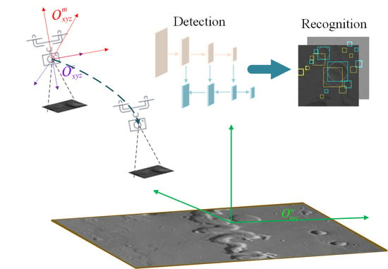
1. Introduction
2. Materials and Methods
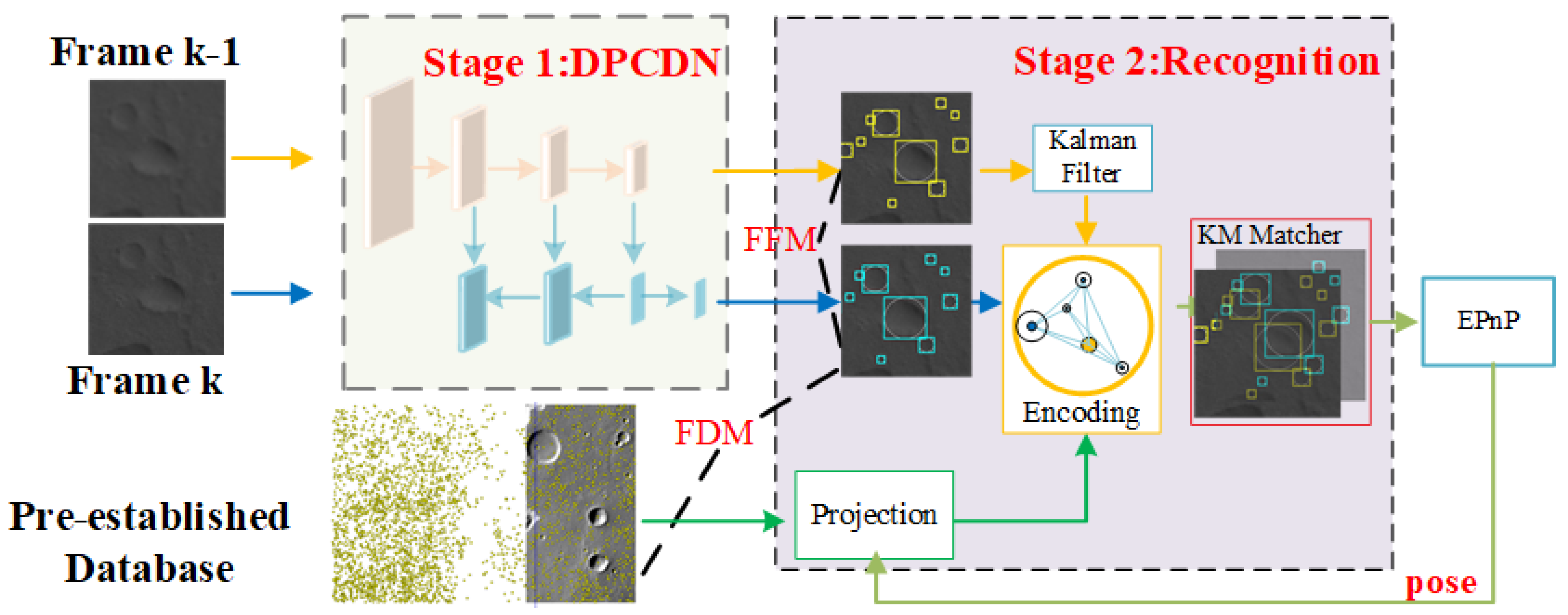
2.1. Methodology
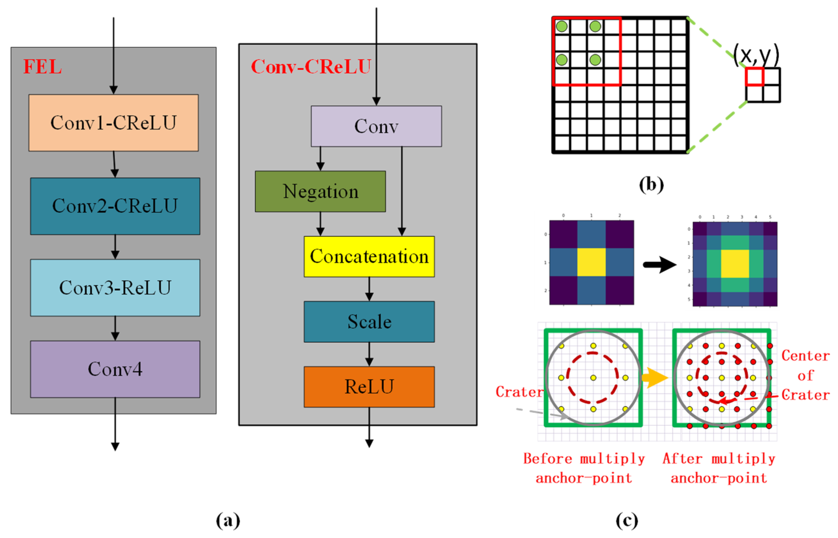
2.2. Stage 1: Crater Detection
2.3. Stage 2: Crater Recognition
- (1)
- Initialize the feature vector , where , and e is the discrete factor.
- (2)
- Using the “constellation” composed of the crater to be matched and m surrounding craters, calculate the angle between the craters, according to ; this process is discretization, and discretization makes the feature more robust.
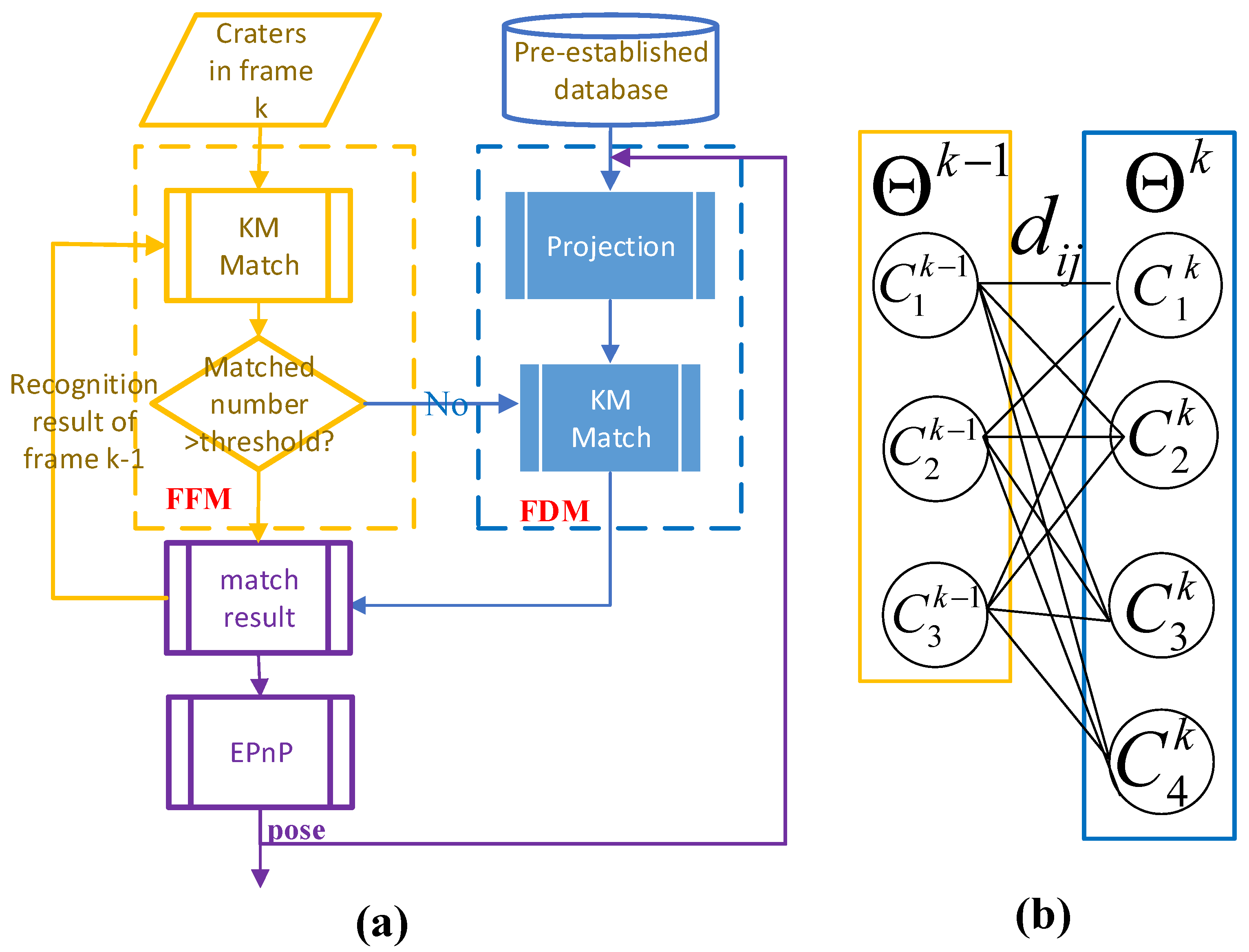
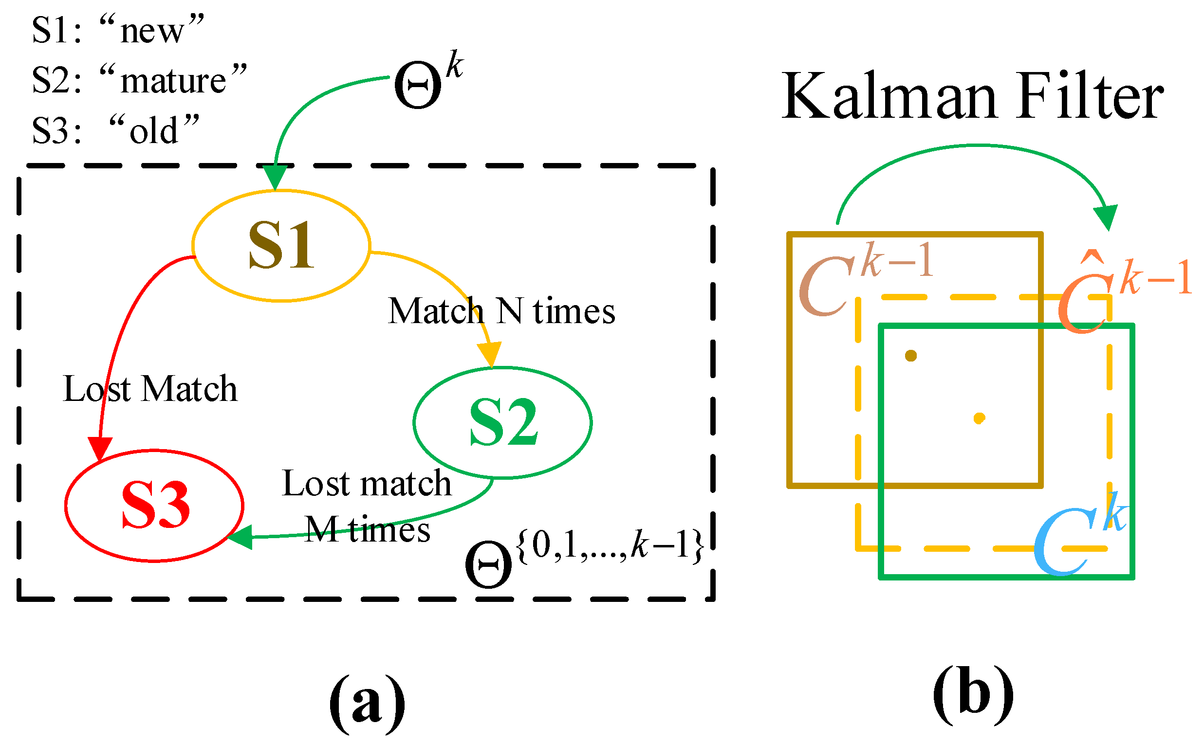
2.3.1. Frame-Frame Match
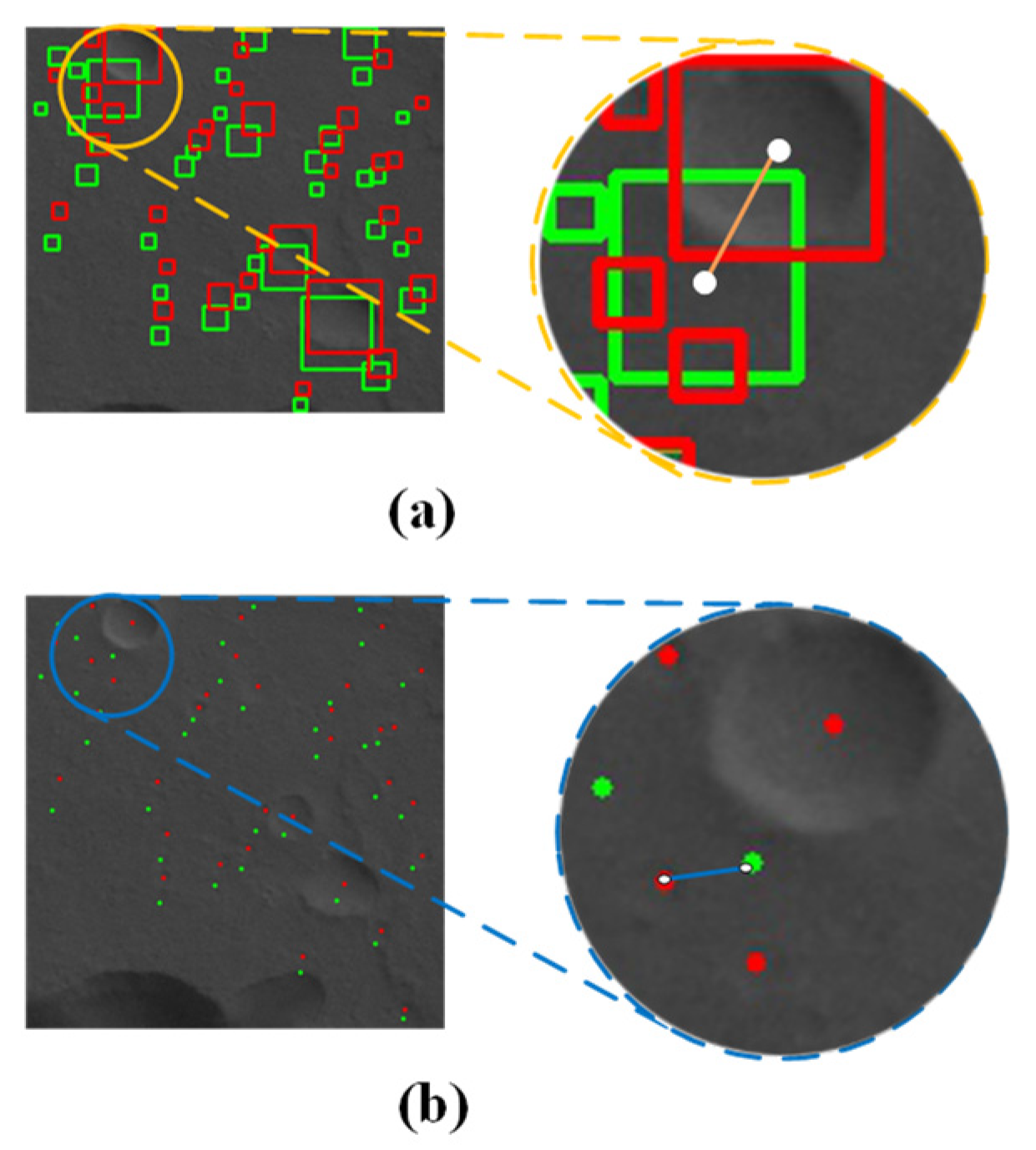
- The Kalman filter calculates the predicted value of the crater . Calculate the IOU between and .
- Encode the feature of craters and calculate the distance between features.
- Input the distance into the KM algorithm, matching craters by IOU first, and match the remaining unmatched craters using the distance of the feature.
- Use successfully matched craters to update the Kalman-filter parameters and update the state of craters in .
2.3.2. Frame Database Match
3. Results
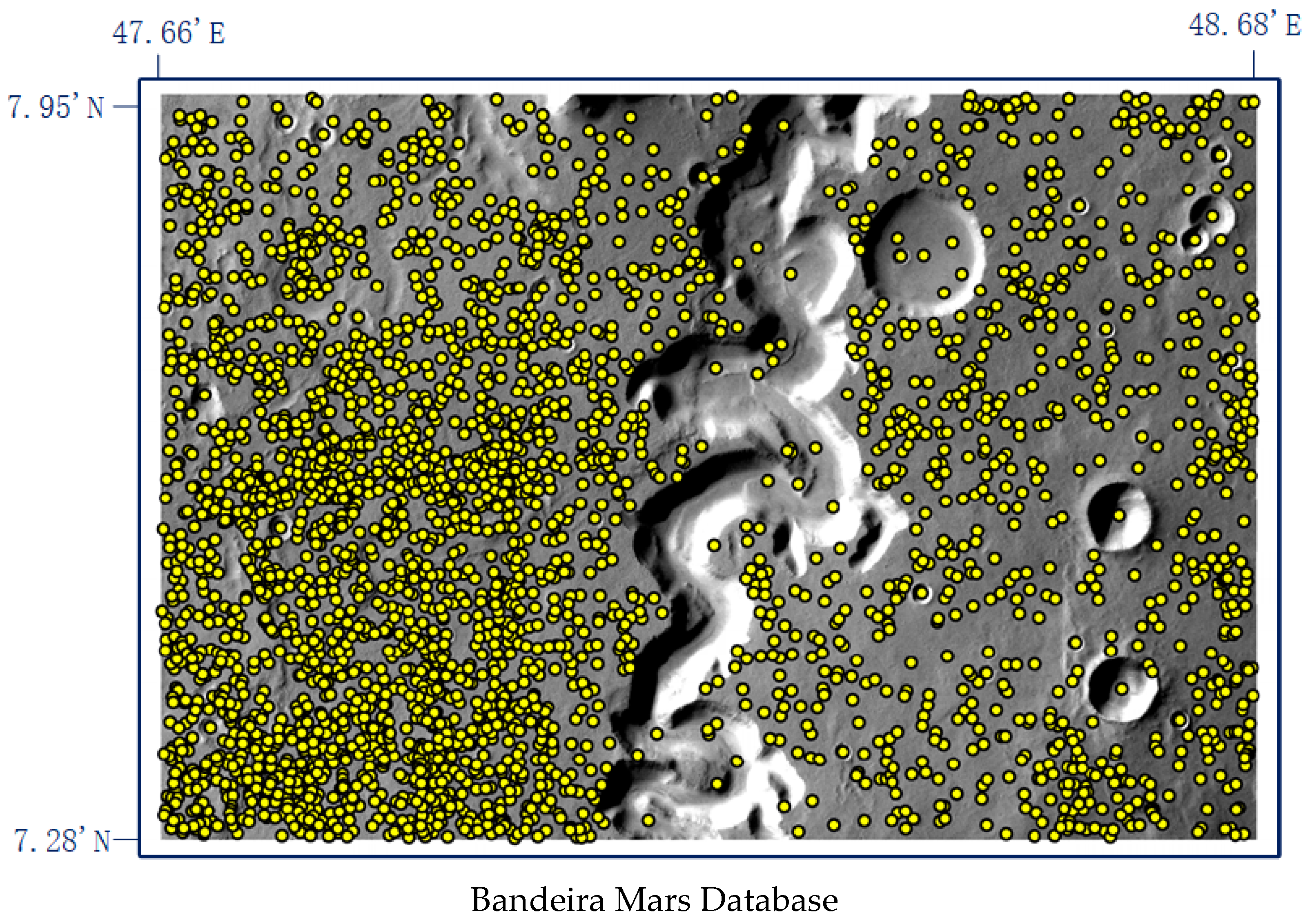
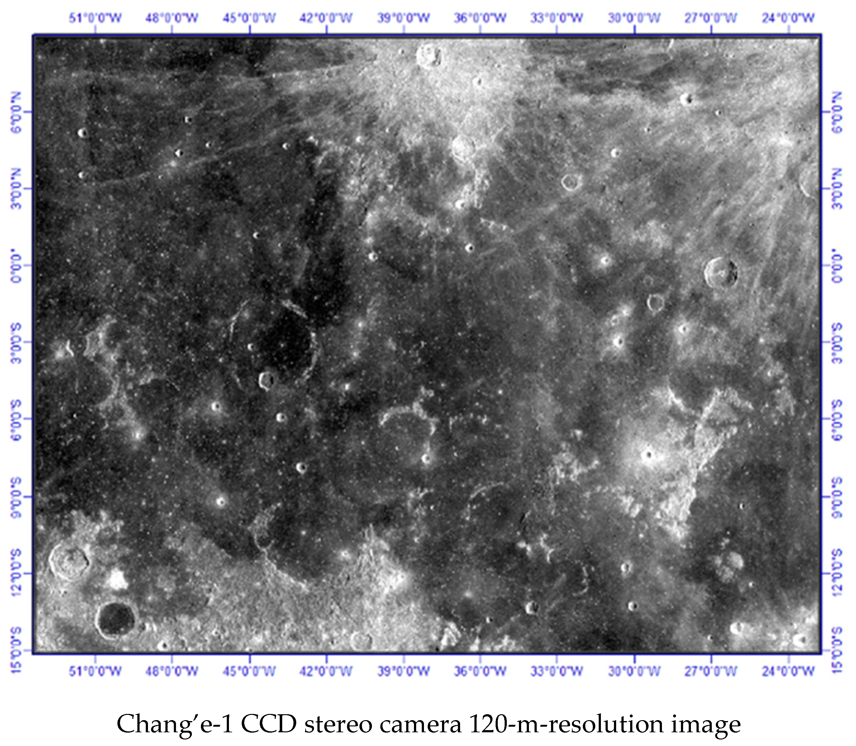
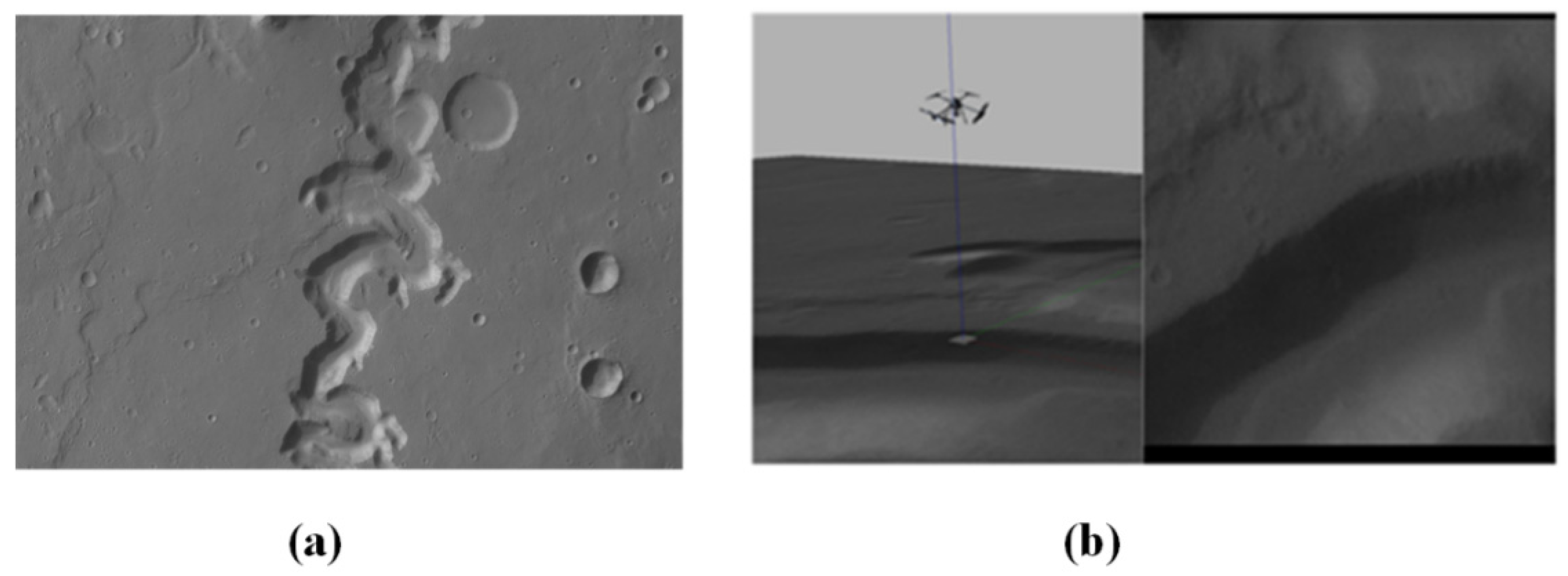
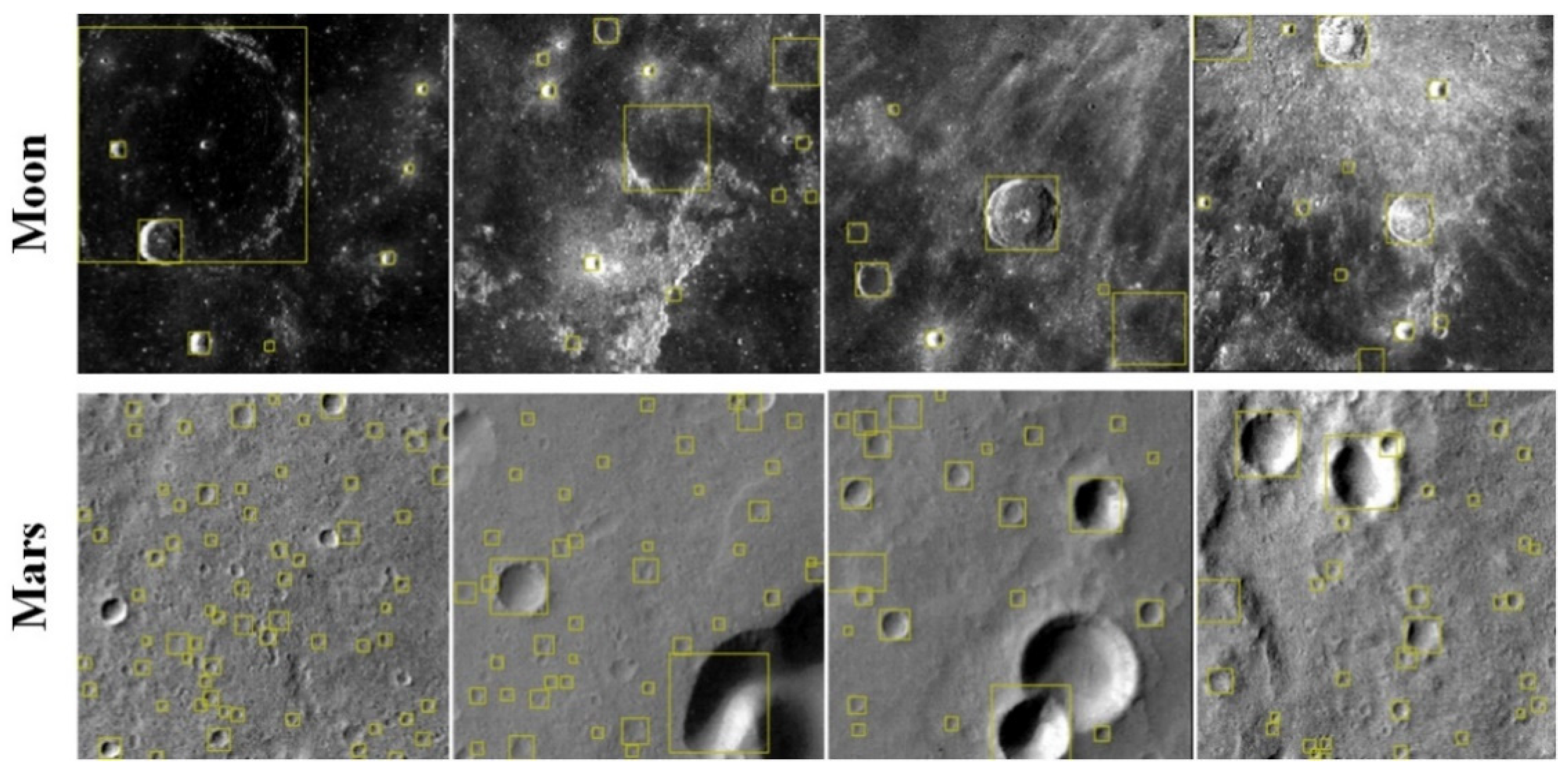
3.1. Experimental Dataset
3.2. DPCDN Validation
3.2.1. Training Details
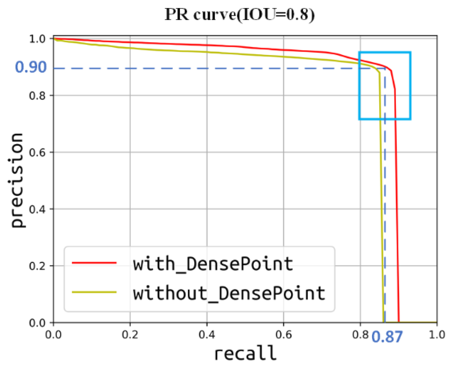
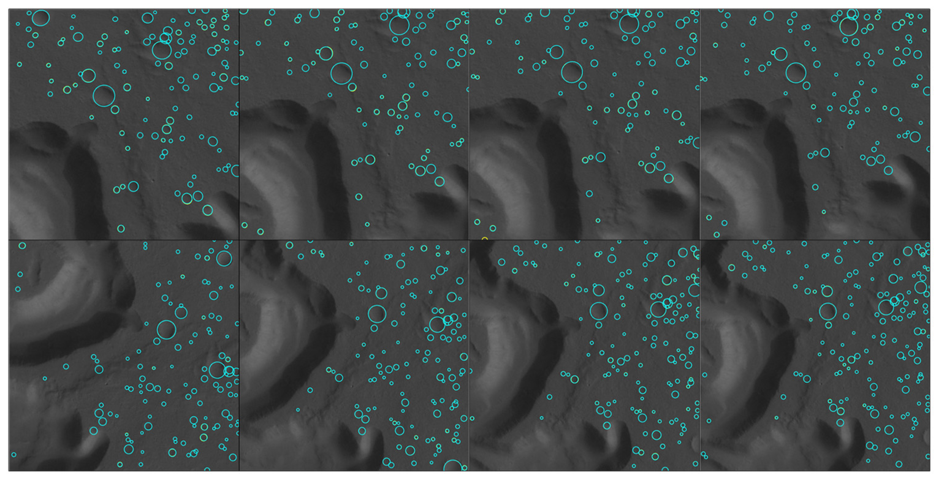
3.2.2. DPCDN Results
3.3. Recognition Validation
3.3.1. Validation of FDM Performance
3.3.2. Validation of FFM Performance
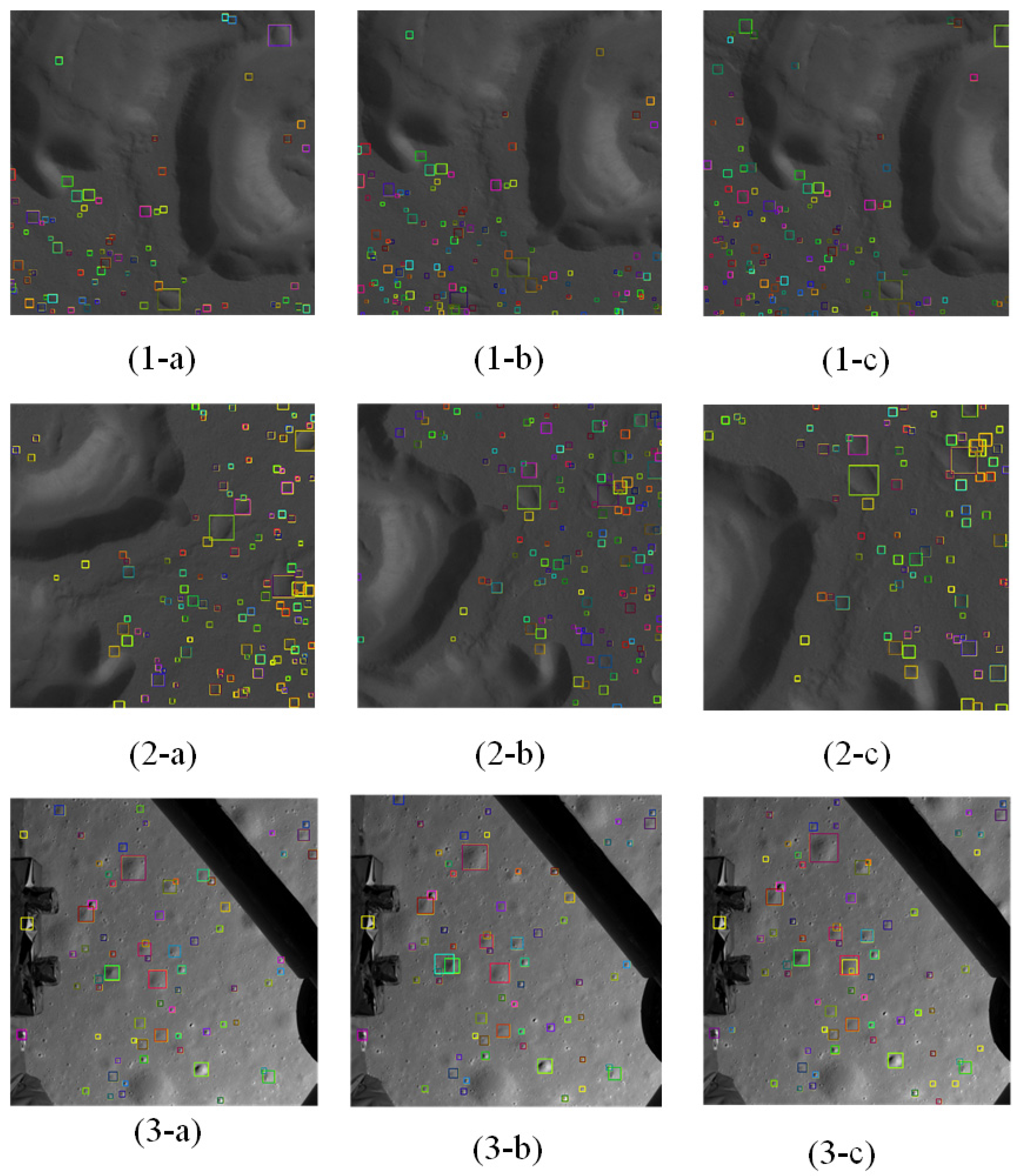
3.3.3. Validation of Recognition
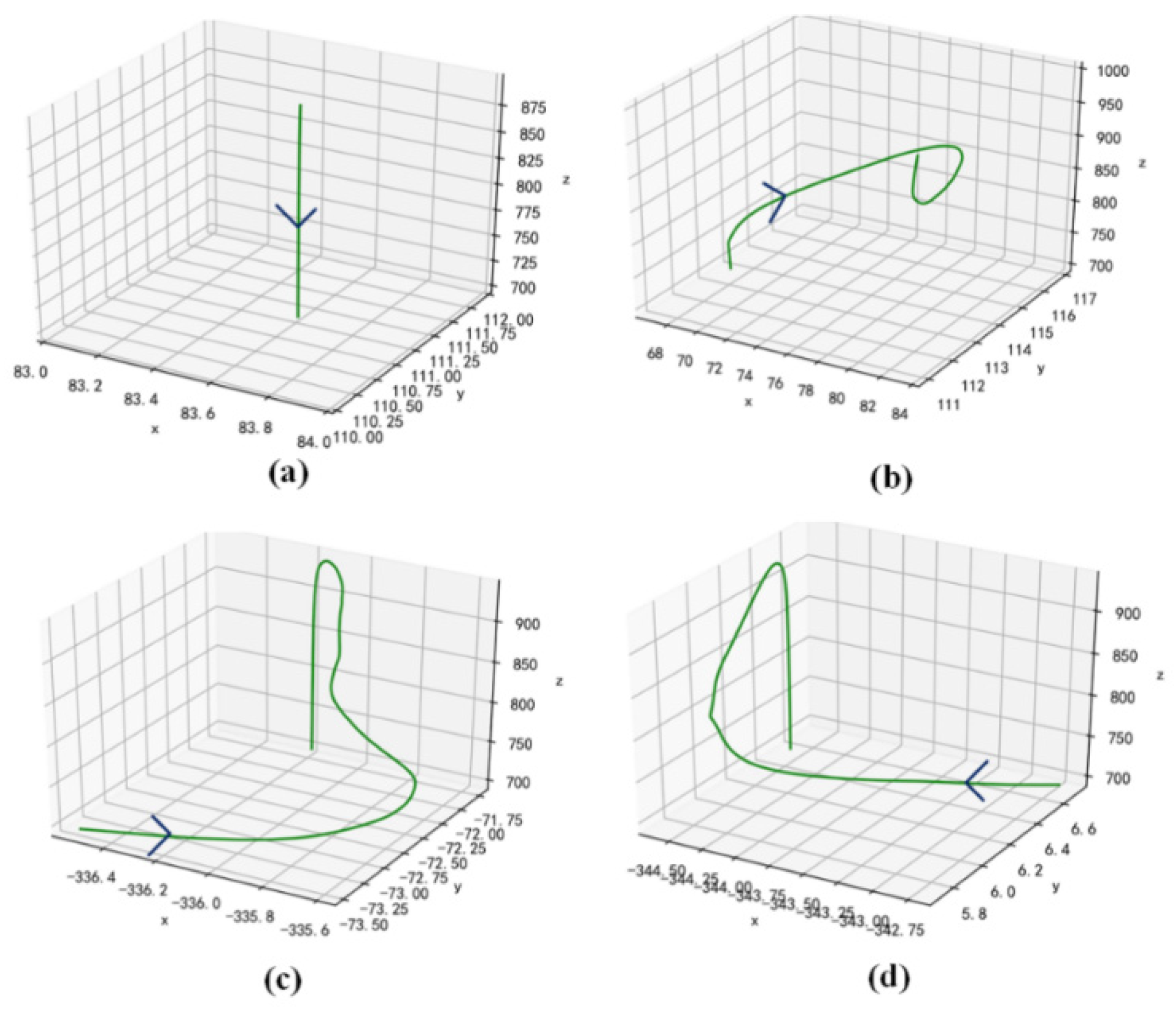
3.4. Pose-Estimation Experiment Results
4. Discussion
5. Conclusions
Author Contributions
Funding
Data Availability Statement
Acknowledgments
Conflicts of Interest
Appendix A
References
- Downes, L.; Steiner, T.; How, J. Lunar Terrain Relative Navigation Using a Convolutional Neural Network for Visual Crater Detection. In Proceedings of the 2020 American Control Conference (ACC), Online, 1–3 July 2020; pp. 4448–4453. [Google Scholar] [CrossRef]
- Johnson, A.E.; Montgomery, J.F. Overview of Terrain Relative Navigation Approaches for Precise Lunar Landing. In Proceedings of the Aerospace Conference, Big Sky, MT, USA, 1–8 March 2008. [Google Scholar]
- Maass, B.; Woicke, S.; Oliveira, W.M.; Razgus, B.; Krüger, H. Crater Navigation System for Autonomous Precision Landing on the Moon. J. Guid. Control Dyn. 2020, 43, 1414–1431. [Google Scholar] [CrossRef]
- James, K. Introduction Autonomous Landmark Based Spacecraft Navigation System. In Proceedings of the 13th Annual AAS/AIAA Space Flight Mechanics Meeting, Ponce, Puerto Rico, 9 February 2003. [Google Scholar]
- Lepetit, V.; Moreno-Noguer, F.; Fua, P. EPnP: An Accurate O(n) Solution to the PnP Problem. Int. J. Comput. Vis. 2009, 81, 155–166. [Google Scholar] [CrossRef] [Green Version]
- Klear, M.R. PyCDA:An Open-Source Library for Autonmated Crater Detection. In Proceedings of the 9th Planetary Crater Consortium, Boulder, CO, USA, 8–10 August 2018. [Google Scholar]
- Ronneberger, O.; Fischer, P.; Brox, T. U-Net: Convolutional Networks for Biomedical Image Segmentation. In Proceedings of the International Conference on Medical Image Computing and Computer-Assisted Intervention, Munich, Germany, 5–9 October 2015. [Google Scholar] [CrossRef] [Green Version]
- Lee, C. Automated crater detection on Mars using deep learning. Planet. Space Sci. 2019, 170, 16–28. [Google Scholar] [CrossRef] [Green Version]
- Downes, L.; Steiner, T.J.; How, J.P. Deep Learning Crater Detection for Lunar Terrain Relative Navigation. In Proceedings of the AIAA SciTech Forum, Orlando, FL, USA, 6–10 January 2020. [Google Scholar]
- Tian, Y.; Yu, M.; Yao, M.; Huang, X. Crater Edge-based Flexible Autonomous Navigation for Planetary Landing. J. Navig. 2018, 72, 649–668. [Google Scholar] [CrossRef]
- Leroy, B.; Medioni, G.; Johnson, E.; Matthies, L. Crater detection for autonomous landing on asteroids. Image Vis. Comput. 2011, 19, 787–792. [Google Scholar] [CrossRef]
- Clerc, S.; Spigai, M.; Simard-Bilodeau, V. A crater detection and identification algorithm for autonomous lunar landing. IFAC Proc. Vol. 2010, 43, 527–532. [Google Scholar] [CrossRef]
- Olson, C.F. Optical Landmark Detection for Spacecraft Navigation. In Proceedings of the 13th Annual AAS/AIAA Space Flight Mechanics Meeting, Ponce, Puerto Rico, 9 February 2003. [Google Scholar]
- Singh, L.; Lim, S. On Lunar On-Orbit Vision-Based Navigation: Terrain Mapping, Feature Tracking Driven EKF. In Proceedings of the Aiaa Guidance, Navigation & Control Conference & Exhibit, Boston, MA, USA, 19–22 August 2013. [Google Scholar]
- Hanak, C.; Ii, T.P.C.; Bishop, R.H. Crater Identification Algorithm for the Lost in Low Lunar Orbit Scenario. In Proceedings of the AAS Guidance and Control Conference, Breckenridge, CO, USA, 5–10 February 2010. [Google Scholar]
- Wang, J.; Wu, W.; Li, J.; Di, K.; Wan, W.; Xie, J.; Peng, M.; Wang, B.; Liu, B.; Jia, M. Vision based Chang’E-4 landing point localization. Sci. Sin. Technol. 2020, 50, 41–53. [Google Scholar] [CrossRef] [Green Version]
- Wang, H.; Jiang, J.; Zhang, G. CraterIDNet: An End-to-End Fully Convolutional Neural Network for Crater Detection and Identification in Remotely Sensed Planetary Images. Remote Sens. 2018, 10, 1067. [Google Scholar] [CrossRef] [Green Version]
- Ren, S.; He, K.; Girshick, R.; Sun, J. Faster R-CNN: Towards Real-Time Object Detection with Region Proposal Networks. IEEE Trans. Pattern Anal. Mach. Intell. 2017, 39, 1137–1149. [Google Scholar] [CrossRef] [PubMed] [Green Version]
- Kuhn, H.W. The Hungarian method for the assignment problem. Nav. Res. Logist. 2010, 52, 7–21. [Google Scholar] [CrossRef] [Green Version]
- Munkres, J. Algorithms for the assignment and transportation problems. SIAM J. 1962, 10, 196–210. [Google Scholar] [CrossRef] [Green Version]
- Lin, T.Y.; Dollar, P.; Girshick, R.; He, K.; Hariharan, B.; Belongie, S. Feature Pyramid Networks for Object Detection. In Proceedings of the 2017 IEEE Conference on Computer Vision and Pattern Recognition (CVPR), Honolulu, HI, USA, 21–26 July 2017. [Google Scholar]
- Shang, W.; Sohn, K.; Almeida, D.; Lee, H. Understanding and Improving Convolutional Neural Networks via Concatenated Rectified Linear Units. In Proceedings of the Ininternational conference on machine learning 2016, New York, NY, USA, 19–24 June 2016; Volume 48, pp. 2217–2225. [Google Scholar]
- Kalman, R.E. A New Approach to Linear Filtering and Prediction Problems. J. Basic Eng. 1960, 82, 35–45. [Google Scholar] [CrossRef] [Green Version]
- Bandeira, L.; Saraiva, J.; Pina, P. Impact Crater Recognition on Mars Based on a Probability Volume Created by Template Matching. Geoscience and Remote Sensing. IEEE Trans. 2007, 45, 4008–4015. [Google Scholar] [CrossRef]
- Robbins, S.J. A New Global Database of Lunar Impact Craters >1–2 km: 1. Crater Location and Sizes, Comparisons with Published Databases and Clobal Analysis. J. Geophys. Res. Planets 2018, 124, 871–892. [Google Scholar]
- Stuart, J.R.; Hynek, B.M. A new global databases of Mars impact craters>1Km:1.Database creation, properties and parameters. J. Geophys. Res. 2011, 117. [Google Scholar] [CrossRef]
- Bandeira, L.; Ding, W.; Stepinski, T.F. Automatic Detection of Sub-km Craters Using Shape and Texture Information. In Proceedings of the Lunar & Planetary Science Conference, Woodlands, TX, USA, 23–27 March 2010. [Google Scholar]
- Koenig, N.; Howard, A. Design and Use Paradigms for Gazebo, an Open-Source Multi-Robot Simulator. In Proceedings of the Intelligent Robots and Systems, Chicago, IL, USA, 14–18 September 2004. [Google Scholar]
- Meier, L.; Honegger, D.; Pollefeys, M. PX4: A node-based multithreaded open source robotics framework for deeply embedded platforms. IEEE Int. Conf. Robot. Autom. 2015, 2015, 6235–6240. [Google Scholar]
- He, K.; Zhang, X.; Ren, S.; Sun, J. Delving Deep into Rectifiers: Surpassing Human-Level Performance on ImageNet Classification. In Proceedings of the 2015 IEEE International Conference on Computer Vision, ICCV 2015, Santiago, Chile, 7–13 December 2015. [Google Scholar]
- Urbach, E.R.; Stepinski, T.F. Automatic detection of sub-km craters in high resolution planetary images. Planet. Space Sci. 2009, 57, 880–887. [Google Scholar] [CrossRef]
- Ding, W.; Stepinski, T.F.; Mu, Y.; Bandeira, L.; Ricardo, R.; Wu, Y.; Lu, Z.; Cao, T.; Wu, X. Subkilometer crater discovery with boosting and transfer learning. Acm Trans. Intell. Syst. Technol. 2011, 2, 1–22. [Google Scholar] [CrossRef] [Green Version]
- Simonyan, K.; Zisserman, A. Very Deep Convolutional Networks for Large-Scale Image Recognition. arXiv 2014, arXiv:1409.1556. [Google Scholar]
- He, K.; Zhang, X.; Ren, S.; Sun, J. Deep Residual Learning for Image Recognition. In Proceedings of the IEEE Conference on Computer Vision and Pattern Recognition, Las Vegas, NV, USA, 27–30 July 2016; pp. 770–778. [Google Scholar]
- Lin, T.Y.; Maire, M.; Belongie, S.; Hays, J.; Zitnick, C.L. Microsoft COCO: Common Objects in Context. In Proceedings of the ECCV 2014—European Conference on Computer Vision, Zurich, Switzerland, 6–12 September 2014. [Google Scholar]
- Wei, Z.; Li, C.; Zhang, Z. Scientific data and their release of Chang’E-1 and Chang’E-2. Chin. J. Geochem. 2014, 33. [Google Scholar] [CrossRef]
- Sturm, J.; Engelhard, N.; Endres, F.; Burgard, W.; Cremers, D. A benchmark for the evaluation of RGB-D SLAM systems. In Proceedings of the Intelligent Robots and Systems (IROS), Vilamoura, Algarve, Portugal, 7–12 October 2012. [Google Scholar]


| Network | Region | ||
|---|---|---|---|
| West | Central | East | |
| Urbach | 67.89% | 69.62% | 79.77% |
| Bandeira | 85.33% | 79.35% | 86.09% |
| Ding | 83.89% | 83.02% | 89.51% |
| CraterIDNet | 90.86% | 90.02% | 93.31% |
| DPCDN | 95.40% | 96.30% | 96.40% |
| FEL | Vgg16 | Resnet18 | |
|---|---|---|---|
| Parameters (Mbits) | 9.7 | 40.3 | 73.3 |
| Speed (fps) | 9.43 | 3.23 | 3.4 |
| Recall (%) | 96.9 | 97 | 97.0 |
| Precision (%) | 97.4 | 97.4 | 97.3 |
| Average F1 score (%) | 97.2 | 97.2 | 97.0 |
| Sequence | Average Crater Density | Accuracy (%) | Error | Speed (fps) |
|---|---|---|---|---|
| Seq1 | 123.1 | 97.0 | 0.196 | 21.65 |
| Seq2 | 89.0 | 96.8 | 0.176 | 17.26 |
| Seq3 | 38.4 | 96.8 | 0.184 | 79.21 |
| Seq4 | 116.2 | 96.5 | 0.185 | 18.80 |
| Average | 91.7 | 97.2 | 0.185 | 34.23 |
| Sequence | Seq1 | Seq2 | Seq3 | Seq4 |
|---|---|---|---|---|
| Accuracy (%) | 99.6 | 96.5 | 99.5 | 98.5 |
| Speed (Only FDM, fps) | 7.41 | 10.84 | 26.61 | 8.11 |
| Speed (FDM + FFM, fps) | 17.34 | 20.07 | 46.93 | 16.56 |
| Sequence | ||||
|---|---|---|---|---|
| Seq1 | Seq2 | Seq3 | Seq4 | |
| APE (m) | 3.93 | 5.89 | 0.11 | 4.74 |
| RPE (m) | 3.26 | 6.02 | 0.15 | 3.84 |
Publisher’s Note: MDPI stays neutral with regard to jurisdictional claims in published maps and institutional affiliations. |
© 2021 by the authors. Licensee MDPI, Basel, Switzerland. This article is an open access article distributed under the terms and conditions of the Creative Commons Attribution (CC BY) license (https://creativecommons.org/licenses/by/4.0/).
Share and Cite
Chen, Z.; Jiang, J. Crater Detection and Recognition Method for Pose Estimation. Remote Sens. 2021, 13, 3467. https://doi.org/10.3390/rs13173467
Chen Z, Jiang J. Crater Detection and Recognition Method for Pose Estimation. Remote Sensing. 2021; 13(17):3467. https://doi.org/10.3390/rs13173467
Chicago/Turabian StyleChen, Zihao, and Jie Jiang. 2021. "Crater Detection and Recognition Method for Pose Estimation" Remote Sensing 13, no. 17: 3467. https://doi.org/10.3390/rs13173467
APA StyleChen, Z., & Jiang, J. (2021). Crater Detection and Recognition Method for Pose Estimation. Remote Sensing, 13(17), 3467. https://doi.org/10.3390/rs13173467