Article

Cross-Domain Scene Classification Based on a Spatial Generalized Neural Architecture Search for High Spatial Resolution Remote Sensing Images

School of Geography and Information Engineering, China University of Geosciences, Wuhan 430078, China
*
Author to whom correspondence should be addressed.
Remote Sens. 2021, 13(17), 3460; https://doi.org/10.3390/rs13173460
Submission received: 20 July 2021 / Revised: 22 August 2021 / Accepted: 25 August 2021 / Published: 1 September 2021

Abstract

:
By labelling high spatial resolution (HSR) images with specific semantic classes according to geographical properties, scene classification has been proven to be an effective method for HSR remote sensing image semantic interpretation. Deep learning is widely applied in HSR remote sensing scene classification. Most of the scene classification methods based on deep learning assume that the training datasets and the test datasets come from the same datasets or obey similar feature distributions. However, in practical application scenarios, it is difficult to guarantee this assumption. For new datasets, it is time-consuming and labor-intensive to repeat data annotation and network design. The neural architecture search (NAS) can automate the process of redesigning the baseline network. However, traditional NAS lacks the generalization ability to different settings and tasks. In this paper, a novel neural network search architecture framework—the spatial generalization neural architecture search (SGNAS) framework—is proposed. This model applies the NAS of spatial generalization to cross-domain scene classification of HSR images to bridge the domain gap. The proposed SGNAS can automatically search the architecture suitable for HSR image scene classification and possesses network design principles similar to the manually designed networks. To obtain a simple and low-dimensional search space, the traditional NAS search space was optimized and the human-the-loop method was used. To extend the optimized search space to different tasks, the search space was generalized. The experimental results demonstrate that the network searched by the SGNAS framework with good generalization ability displays its effectiveness for cross-domain scene classification of HSR images, both in accuracy and time efficiency.

1. Introduction

With the continuous development of satellite sensors, the resolution of remote sensing images is improving, and fine-scale information can be obtained from high spatial resolution (HSR) remote sensing images [1]. However, HSR remote sensing images have many textural, structural, and spectral characteristics [2,3]. These data demonstrate the phenomena of a complex spatial arrangement with high intraclass and low interclass variabilities, giving rise to difficulties in image classification and recognition [4,5]. Pixel-based remote sensing image classification methods frequently consider that the same kinds of ground objects have the same spectral characteristics, while different ground objects in spectral space use separability as the classification premise. Therefore, the pixel-level remote sensing image classification method cannot be effective. The object-oriented classification method is proposed and widely used in HSR images [6,7,8]. The object-oriented classification method can accurately identify the target information and features in HSR remote sensing images. However, the difference between the underlying features and the high-level semantic information still makes the traditional object-oriented image interpretation method unable to obtain the complex semantic information of the important areas in HSR remote sensing images [9]. Eliminating the semantic-gap [10] between low-level features and high-level semantic information to acquire scene semantic information of HSR images has become one of the hot-spots for remote sensing image processing and analysis [11,12].
Scene classification enables obtaining high-level semantic information about different scenes by automatically labelling HSR remote sensing images to establish the relationship between the underlying features and the high-level semantic information [13]. The key to scene classification lies in the extraction of essential features from the images. In recent years, the scene classification method without considering the object prior has been widely used in HSR remote sensing images and can be divided into three main types [14,15]. (1) Scene classification methods based on low-level features. This kind of method extracts the bottom features from the HSR images such as the color, texture, and shape attributes of the image, and uses classifiers to identify scenes. The bottom features can be obtained directly from images without external knowledge including global features [16] and local features [17]. For example, Yang and Newsam compared the scale invariant feature transformation (SIFT) [18] and Gabor texture features. Dos Santos et al. tested a variety of global color and texture features such as color histogram (CH) [19] and local binary pattern (LBP) [20]. However, this method has difficulty in describing the complex spectral and spatial characteristics of ground objects in scenes, thus the classification results are often poor [16,21]. (2) Scene classification methods based on mid-level features. By extracting the local features of the scene, this method maps the local features to the dictionary or parameter space to obtain the mid-level features with stronger discrimination. Then, the mid-level features are input into the classifier to obtain the scene labels [22]. This kind of method mainly includes bag-of-visual-words (BOVW), feature coding, and probabilistic topic models [22,23,24,25]. Luo et al. [23] constructed descriptors for satellite image by connecting color and texture features, and quantified the features of all image blocks into several visual words by K-means clustering. However, the scene classification method based on mid-level features often ignores the spatial distribution between features and lacks the transferability between domains, which greatly limit the expression effectiveness and model universality of HSR image scene classification. (3) Scene classification methods based on high-level features, which automatically extract features from images through training a deep network. Deep learning methods can mainly be divided into two types: supervised feature learning and unsupervised feature learning based methods [26]. With the generalization ability of the deep learning model and the similarity of data between different fields [27,28,29], it is possible to transfer network weight from one domain to another, which is beneficial to network initialization and saves in the time consumption of training [27].
The earliest deep learning method introduced into HSR remote sensing images is the unsupervised feature learning method based on a significant sample selection strategy [30]. The training data of this method is unlabelled. The deep learning method based on supervised features uses labelled image data to train and optimize neural networks to classify images. The CNN is one of the most widely used models in deep learning based on supervised features. According to the development process and direction of CNN scene classification, traditional CNN scene classification methods can be divided into three types [31]: (1) Classical convolutional neural network, for example, AlexNet [32] is composed of a convolution layer, a fully connected layer, and a softmax classifier. VGGNet [33] inherits the framework of LeNet [34] and AlexNet, increasing the depth of the network and obtaining more effective information. These CNN networks have achieved good results in scene classification fields. (2) Convolutional neural network based on the attention mechanism, which means that the neural network uses the attention mechanism to emphasize the useful part more, while inhibiting the less useful part [35,36,37]. (3) Lightweight network. One of the classic models is SqueezeNet [38], which achieves the same accuracy as AlexNet. However, the parameters of SqueezeNet are only one-fiftieth of the parameters of AlexNet. Deep learning, particularly convolutional neural networks (CNNs), has quickly become a popular topic in scene classification applications [39,40,41,42]. In the continuous development of deep learning, a network design principle has been developed for manual design networks. The outcome of this design principle is not only suitable for a single network, but can also be generalized and applied to different settings and tasks.
However, most deep learning-based scene classification methods usually assume that the training and testing data are the same datasets or share the same distribution. In practical applications, since the training and testing data often come from different regions or sensors, the feature distributions are quite different. This phenomenon is referred to as the data shift, and it makes the above assumptions unreliable [43,44]. When faced with new data, manually designed networks often need to once again perform data annotation and network design [43,45,46]. However, data annotation is time-consuming and labor-intensive. Manually designed networks have difficulty adapting well to new datasets or tasks due to insufficient experiments or lack of experience [47]. Inheriting from the architecture of natural image recognition to design a new network is another method in the field of manual design networks [47]. However, the design of the architecture for this method often ignores the characteristics of data without considering the complexity and specificity of HSR images.
A neural architecture search (NAS) method that uses neural networks to automatically search neural network structures [48,49,50,51,52,53] has been proposed. The network searched by the NAS has been applied to large-scale image classification, semantic segmentation, recognition tasks, and scene classification. For example, Barret Zoph et al. [54] proposed a NAS based on reinforcement learning, which used a recursive network to design the network and train the network. The experimental results of the Penn Treebank (PTB) language modelling experiments showed that the model was superior to other advanced models on the PTB dataset. Li et al. [53] proposed the Auto-DeepLab model and studied the semantic segmentation method based on the NAS. Compared to manually designed networks, NASs have the advantages of automatically searching network architectures with high efficiency. However, the traditional NAS has the problem of poor generalization ability and high resource consumption in the search for architectures [55]. The search result of the traditional NAS is to tune a single network instance to a specific setting. The design paradigm of traditional NAS has limitations, which cannot help to discover the general design principles of the network and extend them to different settings [56]. Based on the above problems, He et al. [56] proposed RegNet and found a new general design paradigm of NAS, and the network obtained by RegNet can be generalized in various settings. Under comparable training settings and flops, the RegNet models outperformed the popular EfficientNet models while being up to 5× faster on GPUs. Similar to the manually designed CNN, the traditional NAS often assumes that the features of the training and testing datasets are the same or similar in scene classification. Cross-domain scene classification refers to scene classification tasks in which training sets and test sets come from different distributions. and can help to ameliorate the effect of the data shift [57]. This helps to optimize the model to meet the requirements of practical scene classification application [58,59]. The generalization ability of the model, which refers to the ability of the learned model to predict an unknown dataset, can be evaluated by the results of cross-domain scene classification [44,60,61].
To solve the problem that manual network design is time-consuming and difficult, and the generalization ability of the traditional NAS is poor, a novel neural network search framework—the spatial generalized neural architecture search (SGNAS) framework—was proposed in this paper for HSR image cross-domain scene classification. The SGNAS focuses on the simplification and design of the search space. Within the SGNAS framework, the purpose of this study was to design a simple search space with high efficiency and generalization. Based on the design of the NAS, the setting of its search space was optimized in this study. After optimization, the human-the-loop method was applied to obtain a low-dimensional search space composed of simple networks [56]. To make the search space simpler than the original search space, which essentially aims to improve the search efficiency, a low-computation, low-epoch training regime was used. To ensure that the SGNAS can be applied to different settings and tasks, this study combines the generalization of manual network design principles in the preoptimized and trained search space of the NAS. Based on the designed search space, the model search method integrating the random search strategy with the performance estimation method of training from scratch was used to search the network. Finally, the final model was applied to cross-domain scene classification to verify the generalization ability of the model.
The major contributions of this paper are as follows:
The SGNAS framework was proposed to discover discriminative information from HSR imagery for cross-domain scene classification. Based on the level of search space, the semiautomatic NAS combines the advantages of manual network design, and the traditional NAS was designed. We designed the search space in a low-computation, low-epoch regime, which can be generalized to heavier computation regimes, schedule lengths, and network block types. SGNAS overcomes the bottleneck of the fixed design paradigm of a traditional manual design network and the difficulty of network redesign.
The network searched by SGNAS implements cross-domain scene classification tasks between different datasets in an unsupervised way. In other words, the training and testing datasets will be two groups of different datasets with large differences in characteristics. To search for suitable models for cross-domain scene classification, the evaluation feedback in the performance evaluation was obtained by the cross-domain scene classification in this study.
The rest of this paper is organized as follows. Section 2 introduces the materials and provides a detailed description of the construction of the proposed SGNAS framework. Section 3 introduces the experimental results of the proposed scene classification method. Section 4 discusses the performance of the tested methods further and discusses the possible reasons of misclassification according to the dataset. In Section 5, we draw conclusions from this study.

2. Materials and Methods

2.1. Datasets

This paper used the SIRI-WHU dataset [62], NWPU-RESIST45 dataset [42], UC Merced Land-Use dataset [63], and RSSCN7 dataset [64] for experimental analysis.
The NWPU-RESIST45 dataset is a publicly available remote sensing image scene classification dataset that was created by Northwestern Polytechnical University (NWPU). This dataset contains 31,500 images divided into 45 scene classes. Each class consists of 700 optical images with a size of 256 × 256 pixels. These 45 types of scenes include airplane, airport, baseball diamond, basketball court, beach, bridge, chaparral, church, circular farmland, cloud, commercial area, dense residential, desert, forest, freeway, golf course, ground track field, harbor, industrial area, intersection, island, lake, meadow, medium residential, mobile home park, mountain, overpass, palace, parking lot, railway, railway station, rectangular farmland, river, roundabout, runway, sea ice, ship, snowberg, sparse residential, stadium, storage tank, tennis court, terrace, thermal power station, and wetland. Figure 1 shows representative images of each class.
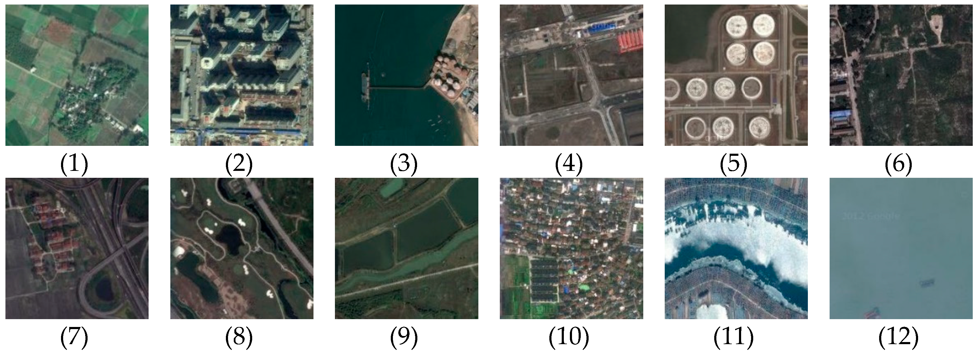
The SIRI-WHU dataset was collected and produced by the research team of Wuhan University, which contains 12 categories of scene images including farmland, business quarters, ports, idle land, industrial areas, grasslands, overpasses, parking lots, ponds, residential areas, rivers, and water. The representative images of each class are shown in Figure 2. Each class in the SIRI-WHU dataset consists of 200 optical aerial images with 200 × 200 pixels and a 2-m resolution. Dataset resources can be searched from Google Earth, mainly covering urban areas of China.
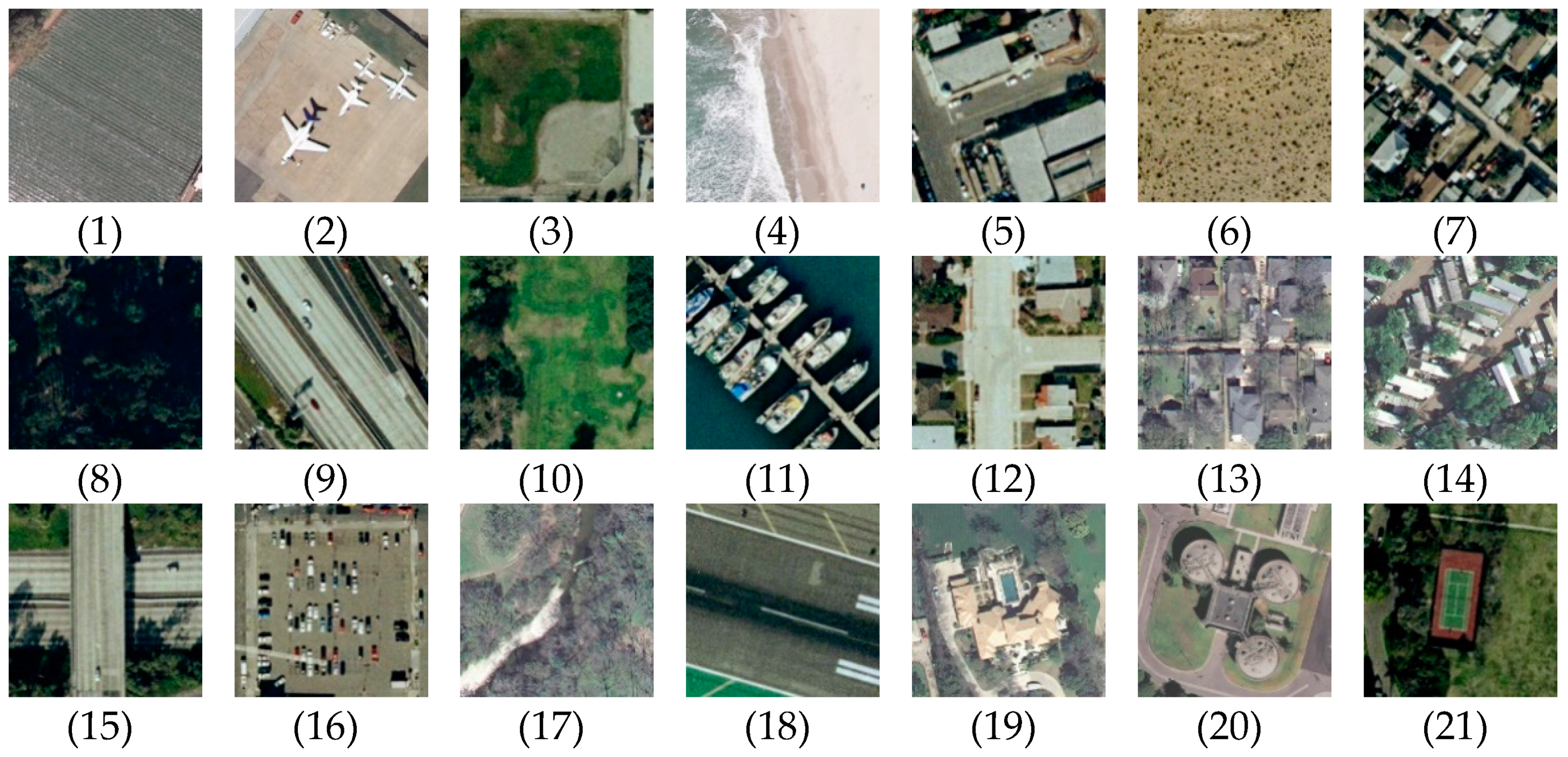
The UC Merced (UCM) dataset is an aerial orthophoto shot from the national geological survey of the United States. It consists of 2100 remote sensing images from 21 scene classes, as shown in Figure 3, including agricultural, airplane, baseball diamond, beach, buildings, chaparral, dense residential, forest, freeway, golf course, harbor, intersection, medium-density residential, mobile home park, overpass, parking lot, river, runway, sparse residential, storage tanks, and tennis courts. Each class in the UCM dataset consists of 200 optical aerial images with 256 × 256 pixels and a 0.3-m resolution.
The RSSCN7 dataset contains 2800 remote sensing scene images, which are from seven typical scene categories: grassland, forest, farmland, parking lot, residential region, industrial region, and river and lake. There are 400 images in each scene type, and each image has a size of 400 × 400 pixels. It is important to note that the sample images in each class are sampled on four different scales with 100 images per scale with different imaging angles. The RSSCN7 dataset is a challenging and representative scene classification dataset due to the wide diversity of the images, which are captured under changing seasons, varying weathers, and sampled on different scales [64], as shown in Figure 4.

2.2. Methods

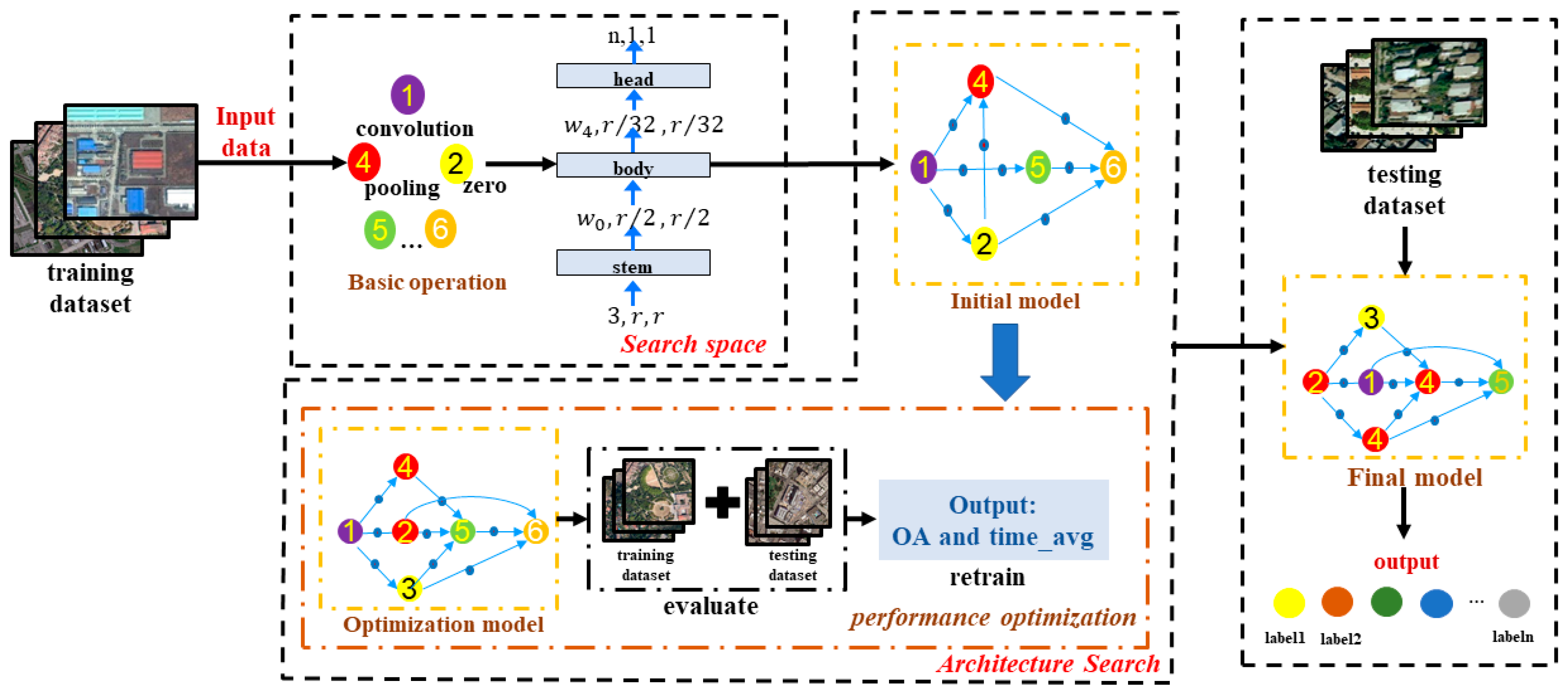
A spatial generalization neural architecture search framework was proposed in this paper for cross-domain scene classification of HSR remote sensing images. As shown in Figure 5, the process of cross-domain scene classification of this paper can be divided into three steps. (1) The architecture search space is designed. (2) The designed search space searched network for HSR images dataset. The HSR image dataset is used as a search dataset and input into the designed search space to search for networks in this step. The model is continuously optimized through the performance evaluation feedback until the final model is obtained. (3) The network obtained by the search space is used for cross-domain scene classification to verify the generalization ability. An HSR image dataset is used as the training dataset, and another HSR dataset different from the training set is used as the testing dataset. Finally, through cross-domain scene classification, the category labels of different images will be output.

2.2.1. Search Space

A low-dimensional and simple search space was designed in this paper. The architecture suitable for cross-domain scene classification of HRS remote sensing images was searched based on the designed search space. The search space combines the generalization of manually designed networks, which can generalize them in various networks and tasks. The purpose of this study was to optimize the problems existing in the manually designed network and traditional NAS. After designing a simple and low-dimensional search space, the generalization ability of the search space was evaluated. He et al. verified the search space of Regnet [56] and found that the search space had no signs of overfitting under the conditions at higher flops, higher epochs, with 5-stage networks, and with various block types. These phenomena indicate that the search space can be extended to new settings. Liu et al. also used Regnet as a comparison network for image classification in the field of computer vision [65]. Inspired by the above research, a network search space that combines the advantages of manual designed network and traditional NAS was designed in this research. The search space also retained the semiautomatic performance of traditional NAS, which can search a good network for the specific architecture automatically. The essence of SGNAS is a semiautomatic NAS combined with the generalization ability of the manual design network. Section 2.2.1 can be divided into two parts: (A) Design of the search space and (B) search space quality detection.

A. Design of the Search Space

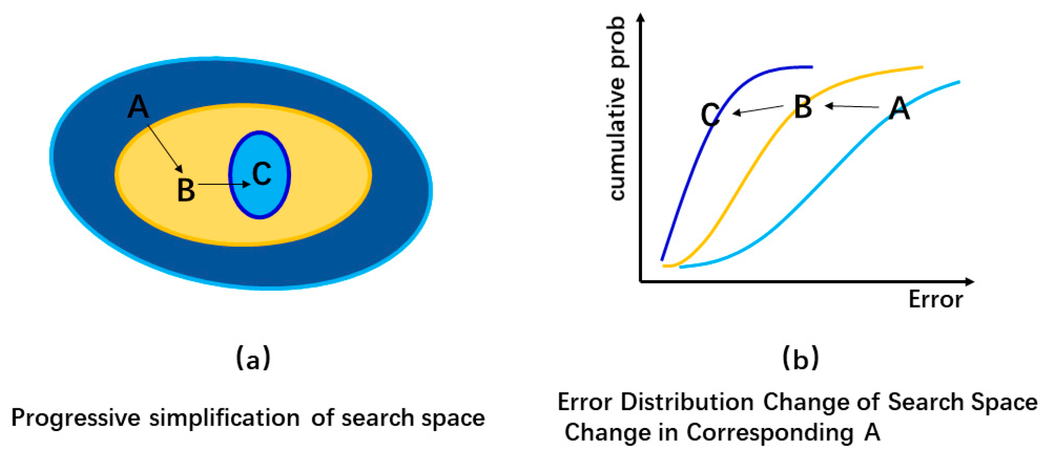
The search space of SGNAS will define a series of basic network operations (convolution, fully connected layer, average pooling, and residual bottleneck block) and connect these operations to form an effective network. The design of the search space in this study is a process of gradual simplification of the initial search space without constraints [56]. A simple schematic diagram of the design concept is shown in Figure 6 [56].
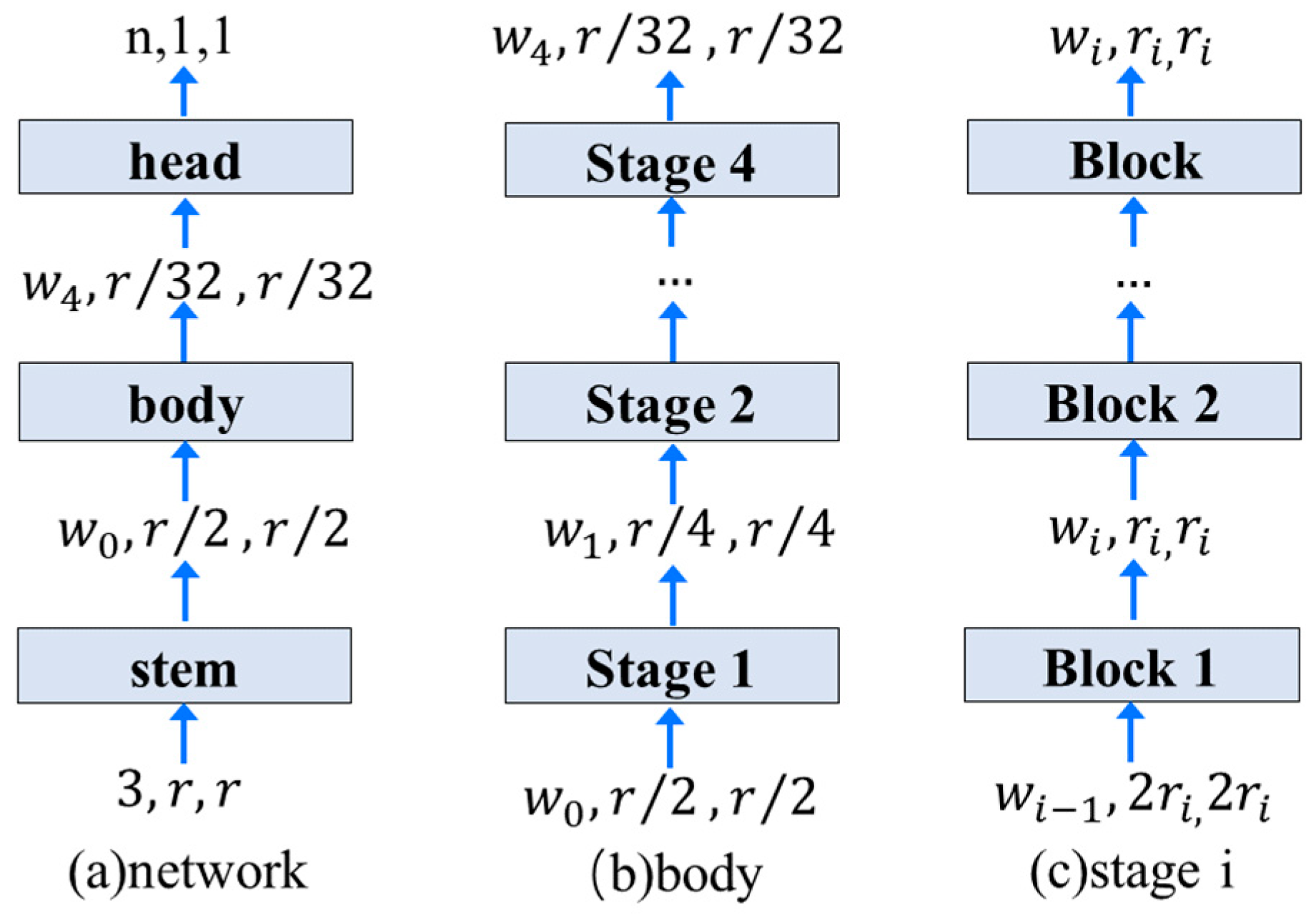
Figure 6a shows that the search space was simplified gradually from A to B to C in the design of the search space in this paper. The error distribution was strictly from A to B to C, as is shown in Figure 6b. Each design step was used to search for a simpler and more efficient model than before. The input was the initial search space without constraints in this paper, while the model output was simpler, had lower computational cost, and better performance than the previous model. The basic network design of the initial search space was also very simple (as shown in Figure 7 [56]). The search space was composed of the body that was used to perform the calculation, stem, and full connection layer (head) for predicting output types (as shown in Figure 7a), and we set the input picture to 224 × 224 × 3 in this study. The stem is a convolution layer, where the convolution kernel was 3 × 3, the number of convolution kernels was 32, and the value of strides was 2. The head was a fully connected layer, which was used to output n categories. The body was composed of four stages. From stage 1 to stage 4, the resolution gradually halved (as shown in Figure 7b). However, the number of characteristic graphs output by each stage, which are ω 1 ,     ω 2 ,     ω 3 , and ω 4 , needs to be searched as hype-parameters in the search space. Each stage was composed of d i identical blocks (as shown in Figure 7c).
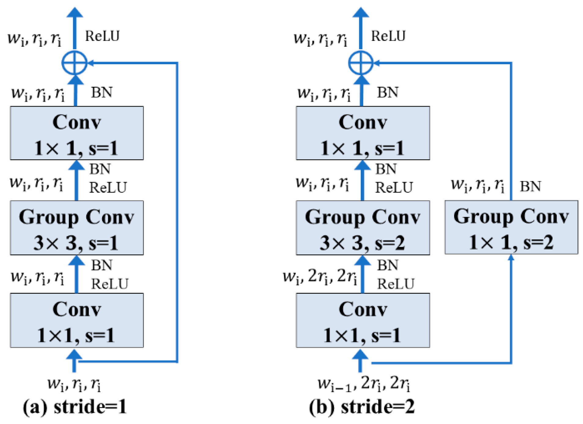
The block used in this paper was the residual bottleneck block [56,66], which is the block of the halved width and halved height of the output feature map (as shown in Figure 8). The main branch of the block is a 1 × 1 convolution (including BN and ReLU), a 3 × 3 group convolution (including BN and ReLU), and a 1 × 1 convolution (including BN). On the branch of the shortcut, when stride = 1, no processing is performed. When stride = 2, it is down-sampled through a 1 × 1 convolution (including BN) [56]. The number of blocks also needs to be searched. Three parameters need to be searched in the residual bottleneck block: the number of channels of block ( ω 1 ), cell group width (the number of horizontal repeats of block, g i ), and the parameter that is used to determine the number of characteristic graphs inside the block (bottleneck ratio b i ). Generally, there are four stages in the network, while the parameters that need to be determined in each stage are d i and ω i , b i , g i . Therefore, the optimal setting of 16 parameters is needed to design the search space.
Following the settings of [56], this study limited the initial values of ω i , d i , b i , and g i to ω i   1024, d i   16, b i {1,2,4}, g i {1, 2, …, 32}. The network key parameters were extracted from the above range by log-uniform sampling, and the quality of search space was judged by EDF function [56]. After that, the search space of SGNAS was continuously optimized and updated by updating the factors such as the sharing bottleneck rate, sharing group width, increasing the number of channels, and increasing the number of blocks. The accuracy of the model will not be lost due to the change in the above factors, as can be proven by determining the quality of the search space. In contrast, the search range of the search space can be greatly reduced, and the search efficiency can be improved by sharing the group width. The performance of the architecture can be improved by increasing the number of channels and blocks. On the basis of the previous optimization and the results obtained by setting AnyNetB, AnyNetC, AnyNetD, and AnyNetE in [56], it can be found that the number of channels of the block ( ω 0 ) has a linear relationship with the index of blocks in the search space of the SGNAS. The linear function is:
μ j = ω 0 + ω s j ( 0 < j < d )
The three parameters in the equation are the initial width ω 0 , slope ω s , and block width μ j for each j < d. To quantize μ j , this study used an additional parameter ω m > 0. Then, S j can be computed for each j:
μ j = ω 0 ω m S j
S j = l o g ω m μ j ω 0
To quantify μ j , we will round S j (denoted by S j ) and compute quantized per-block widths ω j :
ω j = ω 0 ω m S j
Based on the above, there were three more parameters in the design of the search space: ω 0 , ω s , and ω m . However, the search space can be further limited from 16 parameters to six parameters through the previous analysis; these parameters are d i , ω 0 , ω s , ω m , b i , and g i , and the reduction in the number of parameters greatly improves the search efficiency of the search space. This study restricts the values: d i < 64, ω 0 < 256, ω s < 256, ω m   [1.5, 3], b i   {1, 2, 4} and g i   {1, 2, …, 32}, which follows the setting of [56]. The search space will be simplified by using the human-the-loop method after the basic setting of the search space is completed. The simplification of the search space aims to obtain a search space with low computational cost and low number of epochs, in order to improve the computational efficiency of the search space. Based on the original low-dimensional and simple search space, this study completed the generalization setting based on the design of Regnet [56]. The finished SGNAS is a semiautomatic network architecture.

B. Search Space Quality Detection

The search space designed in this paper was an enormous space containing many models. We can sample the model from a search space to generate a model distribution and then use classical statistical tools to evaluate the search space. In this study, an error empirical distribution function (EDF) [67] was used to detect the quality of the design space. When n models are sampled in the search space and the error is m i , EDF is:
F ( m ) = 1 n i = 1 n 1 [ m i < m ]
where F(m) is the model proportion when the error is less than m.

2.2.2. Architecture Search

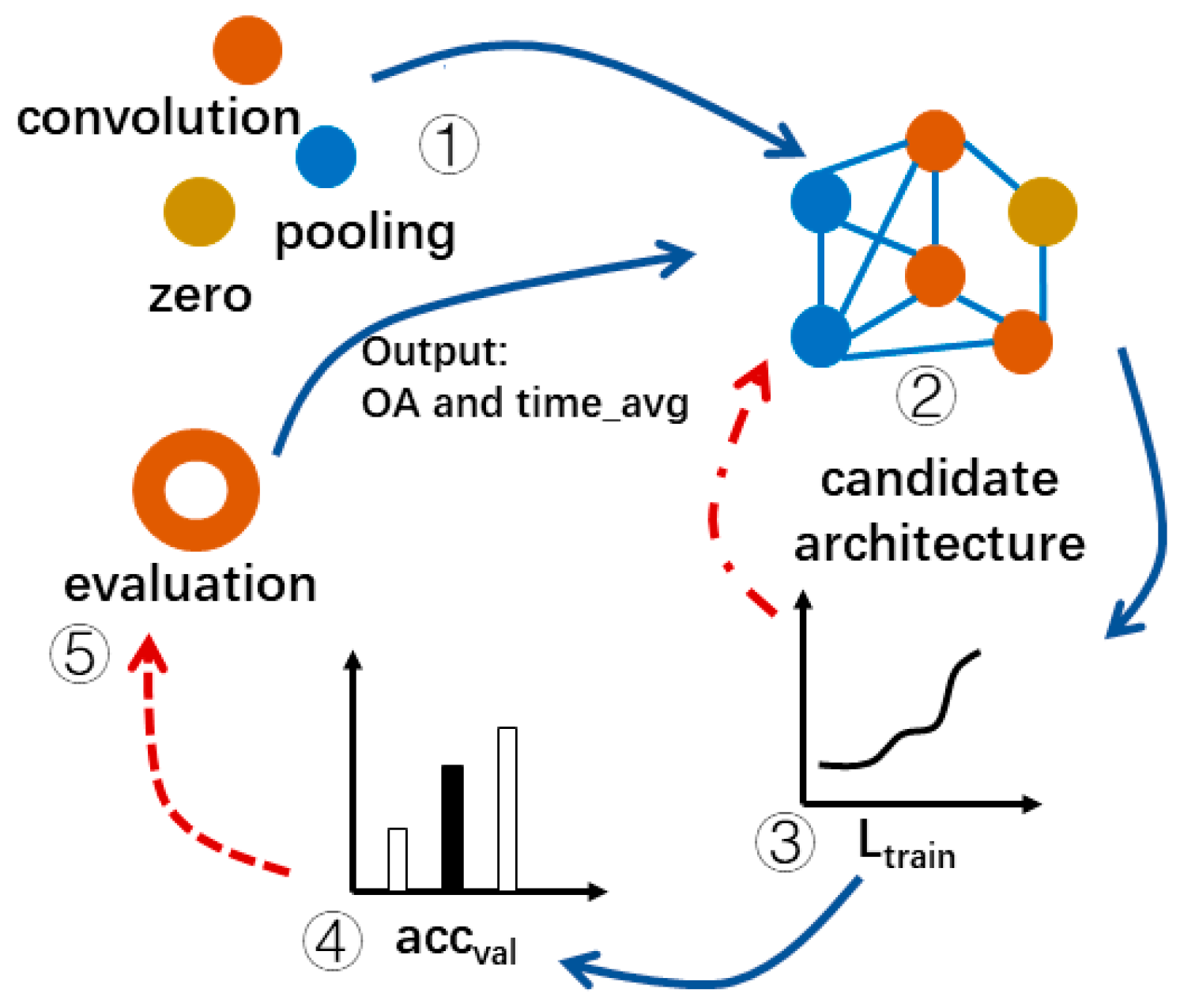
After the search space of the SGNAS is designed to be complete, the framework will be used to search the cross-domain scene classification network of the corresponding dataset. The search process can be divided into three steps: (1) The HSR remote sensing image dataset to be searched is input into the network architecture, and the suitable network is searched according to the different data sets; (2) suitable candidate models are searched for cross-domain scene classification automatically with low computing resources and great global optimization performance; and (3) the overall accuracy (OA) and the inference time (Time_infer) are used to evaluate the accuracy and computational performance of the search network. The whole process is repeated until the final model is found. After the network is obtained by using the framework of SGNAS, the model needs to be retrained by using the search datasets. The purpose of model retraining is to optimize the parameters of the model and obtain a more suitable model for cross-domain scene classification. Finally, a function is added to the searched model since the traditional NAS usually searches models for natural images, which is used to load the HSR remote sensing images for the model; thus, the model can be used for scene classification of HSR remote sensing images. Figure 9 shows the general steps of a network search by the SGNAS. Section 2.2.2 can be divided into two parts: (A) Search strategy and (B) Performance estimation.

A. Search Strategy

The proposed framework proposed is different to traditional NAS. However, the essence of the SGNAS is still a NAS combined with the generalization of a manual design network, which is still a neural network for searching network architecture by using a neural network. Therefore, the architecture is divided into three parts, similar to the traditional NAS: search space, search strategy, and performance estimation. Since the search space was optimized during the design of the search space in this study, thus improving the search efficiency of the framework, the search strategy adopted in this study was a simple random search strategy. Random search is the simplest search strategy, which randomly selects an effective candidate architecture from the search space and does not involve a learning model. However, it has been proven to be very useful in hype-parameter search [54].

B. Performance Estimation

The evaluation step is shown in Figure 9 and requires an effective performance estimation method. The simplest performance estimation method of training from scratch is used to measure the accuracy of the searched model through experiments [54], which is used to obtain feedback to optimize the search algorithm. The proposed framework uses this feedback to retrain the network obtained from the previous search, in order to optimize the model parameters of the model searched previously. Then, a model that is more suitable for cross-domain scene classification can be obtained. Although this method is slow, the search space of the SGNAS is carried out in a low-computation, low-epoch regime, which greatly improves the computing speed.

2.2.3. Cross-Domain Scene Classification

The SGNAS was used to search for the image features of the HSR remote sensing image dataset, in order to obtain the final model suitable for cross-domain scene classification of the searched dataset. The searched model will be migrated to different datasets for cross-domain scene classification to obtain the final classification results, which aims to verify the spatial generalization of the model obtained by the proposed framework. Specific experimental settings and experimental results are shown below.

3. Results

Cross-domain scene classification experiments between different datasets were used to verify the generalization of the framework and confirm the complexity of the SGNAS in order to avoid overfitting. The quantitative and computational performance of the searched network were evaluated by overall accuracy (OA), confusion matrix, and inference time (Time_infer).

3.1. Experimental Setup

3.1.1. Implementation Details

The experiments were implemented using PyTorch. The cross entropy loss function (CrossEntropyLoss) was used as the loss function. The learning rate was initially set to 1e-5 with a weight decay of 5e-6. The mini-batch size was set to eight, and the normalization parameter was set to 5e-5. All models were trained on four NVIDIA RTX2080 GPUs. To verify the spatial generalization ability of the proposed model, we established three cross-domain scenarios termed as UCM→RSSCN7, SIRI-WIIU→RSSCN7, and NWPU-RESIST45→RSSCN7, referring to source domain→target domain for data analysis. As the training set and test set of this experiment came from two different datasets, there were large differences in image types, scales, and contents. To match the seven types in the RSSCN7 dataset, for the UCM dataset, this experiment selected the corresponding seven similar types for the experiment: golf course, agricultural, storage tanks, river, forest, density residential, and parking lot. For the SIRI-WHU dataset, industrial areas, farmland, parking lots, residential areas and rivers were selected to correspond to the five types of industrial region, farmland, parking lot, residential region, and river and lake in the RSSCN7 dataset. Seven similar types were selected from the NWPU-RESIST45 dataset for the experiments: dense residential, forest, golf course, industrial area, parking lot, rectangular farmland, and river. The experiments of AlexNet, Vgg16, ResNet50 [68], and ENAS [69] on the same cross-domain scenario settings were used for comparative validation.

3.1.2. Evaluation Metrics

The OA, inference time, and confusion matrix are employed as the evaluation standard of the cross-domain scene classification. The OA is defined as the number of correctly classified images divided by the total number of images. The inference time implies the inference efficiency of the trained model to make predictions against previously unseen data, and is used as an evaluation metric to validate the efficiency of different models in the experiment. The confusion matrix is an informative table used for analyzing the confusions between different scene classes. It is obtained by counting the correct and incorrect classifications of the test images in each class and accumulating the results in a table.

3.2. Experiment 1: UCM→RSSCN7

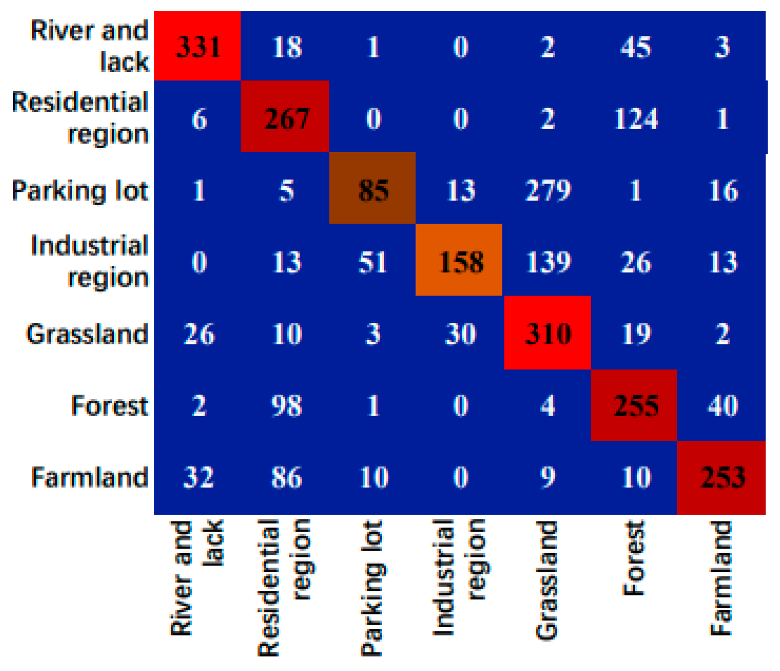
The UCM dataset was used as the training set, and the RSSCN7 dataset was used as the test set in this section to conduct the cross-domain scene classification experiment. The accuracy and the inference time comparison between SGNAS and other models is shown in Table 1, and the accuracy of each scene is shown in Table 2. Figure 10 shows the confusion matrix of the classification results.
Table 1 shows that the experimental results of the model searched by the SGNAS were superior to those of the models used for comparison (i.e., the manually designed Vgg16, AlexNet and ResNet50) and the network searched by ENAS. From Table 2 and Figure 10, it can be seen that the overall classification accuracy of river and lake was the highest, with the classification accuracy of 82.75%, while the parking lot and industrial regions had lower accuracy. The classification accuracy of the parking lot was 21.25%, and that of the industrial region was 39.50%. However, among the seven scenes, the classification accuracies of five scenes were over 60%. As can be seen in the confusion matrix, there was some confusion between certain scenes. For instance, some scenes belonging to the parking lot were classified as grassland. The inference time used by this framework was less than that of the other models used for comparison, as shown in Table 1. This indicates that the proposed SGNAS framework is a promising avenue for efficient cross-domain scene classification.

3.3. Experiment 2: SIRI-WIIU→RSSCN7

This experiment uses the SIRI-WHU dataset as the training set and the RSSCN7 dataset as the test set to conduct the cross-domain scene classification experiment. The accuracy and the inference time comparison between SGNAS and other models is shown in Table 3, and the accuracy of each scene is shown in Table 4. Figure 11 shows the confusion matrix of the classification results.
As shown in Table 4, the farmland class acquires the highest classification accuracy of 79.75%. However, the classification accuracy of the industrial area was only 8.25%. In a total of five types of scenes, the classification accuracies of more than half of the scenes were above 60%. According to the confusion matrix in Figure 11, the proposed model showed some confusion between industrial regions and farmland and between industrial regions and parking lot spaces. The reasons are discussed and explored in Section 4. As shown in Table 3, although the inference time of SGNAS was slightly longer than that of AlexNet and close to that of Vgg16, the OA of SGNAS far transcended that of AlexNet and Vgg16. In addition, the proposed SGNAS framework acquired both better OA and time efficiency compared to ResNet50 and ENAS. This indicates that the proposed SGNAS framework is able to achieve a satisfying balance between the scene classification generalization ability and time efficiency.

3.4. Experiment 3: NWPU-RESIST45→RSSCN7

The NWPU-RESIST45 dataset was used as the training set and the RSSCN7 dataset was used as the test set to conduct the cross-domain scene classification experiment in this section. The accuracy and the inference time comparison between SGNAS and other models is shown in Table 5, and the accuracy of each scene is shown in Table 6. Figure 12 shows the confusion matrix of the classification results.
As shown in Table 6, the proposed SGNAS performed well in all scenes except for the residential regions, and showed particularly good performance for farmland, which had the highest classification accuracy. The classification accuracy of farmland was 91.75%, while that of residential regions was only 20.75%, as can be seen in Table 6. According to the confusion matrix in Figure 12, the proposed model displayed misclassification between farmland and forest, and between farmland and residential regions. AlexNet had the shortest inference time, but the OA of the proposed SGNAS was better than that of AlexNet. ResNet50, Vgg16, and ENAS had longer inference time than SGNAS, as shown in Table 5. The overall classification accuracy of SGNAS was the highest, and it is far superior to Vgg16 and ENAS, as shown in Table 5. This confirms that the proposed framework shows an effective generalization ability compared with the manual designed network and traditional NAS for comparison.
ClassAccuracy (%)
Farmland91.75
Forest52.50
Grassland62.25
Industrial region74.75
Parking lot76.75
Residential region20.75
River and lake60.00

4. Discussion

4.1. Visual Comparative Analysis of Cross-Domain Scene Classification Results

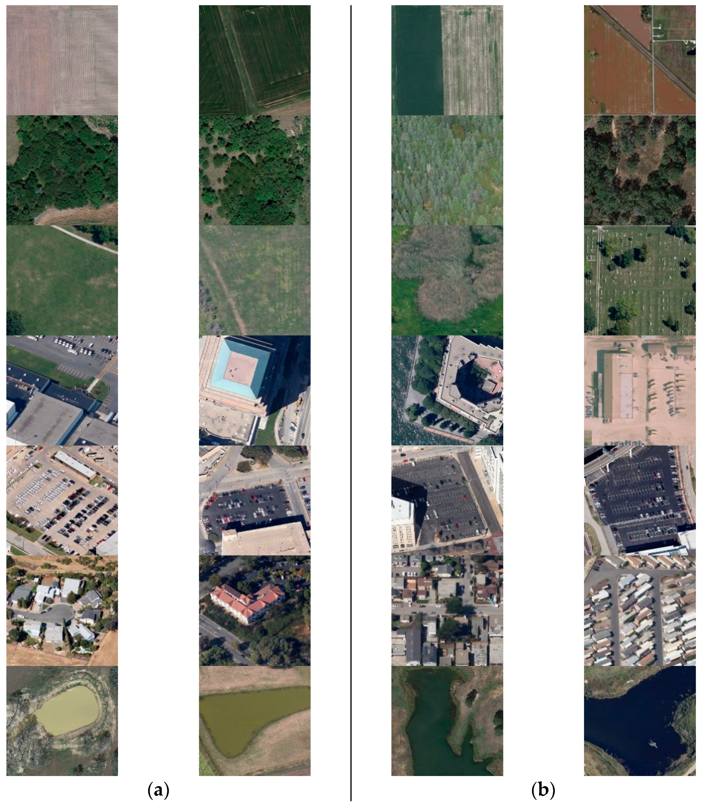
This section focuses on exploring the reason of misclassification through HSR images, on the basis of the confusion matrix and experimental results in Section 3. Figure 13 shows the examples of the main confusion between UCM, SIRI-WIIU, NWPU-RESIST45 dataset, and RSSCN7 dataset.
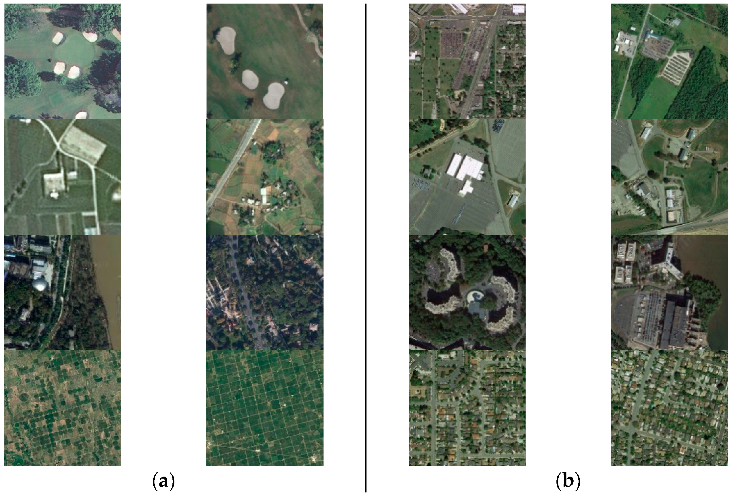
In the experiments of UCM→RSSCN7, there was some confusion between parking lots and grass scenes. This can be explained by the first line in Figure 13, where the golf course in the UCM and the parking lot in the RSSCN7 dataset were similar in spectrum feature. In addition, the two categories were composed of the same objects such as grass and bare ground. For SIRI-WHU→RSSCN7, there was some confusion between farmland and parking lots and industrial region. This can be explained by the fact that the pairs of classes had similar spectral or structural features, which are shown in the second and third rows of Figure 13. Both parking lot in the SIRI-WHU dataset and industrial region in the RSSCN7 dataset feature vegetation cover. In the experiments of NWPU-RESIST45→RSSCN7, the scenes of residential region and farmland had some misclassification. This is due to the similar spatial distribution or spectral characteristics of the categories in different datasets, for example, both residential regions and farmland featuring vegetation cover had a similar texture, as shown in the last row in Figure 13.
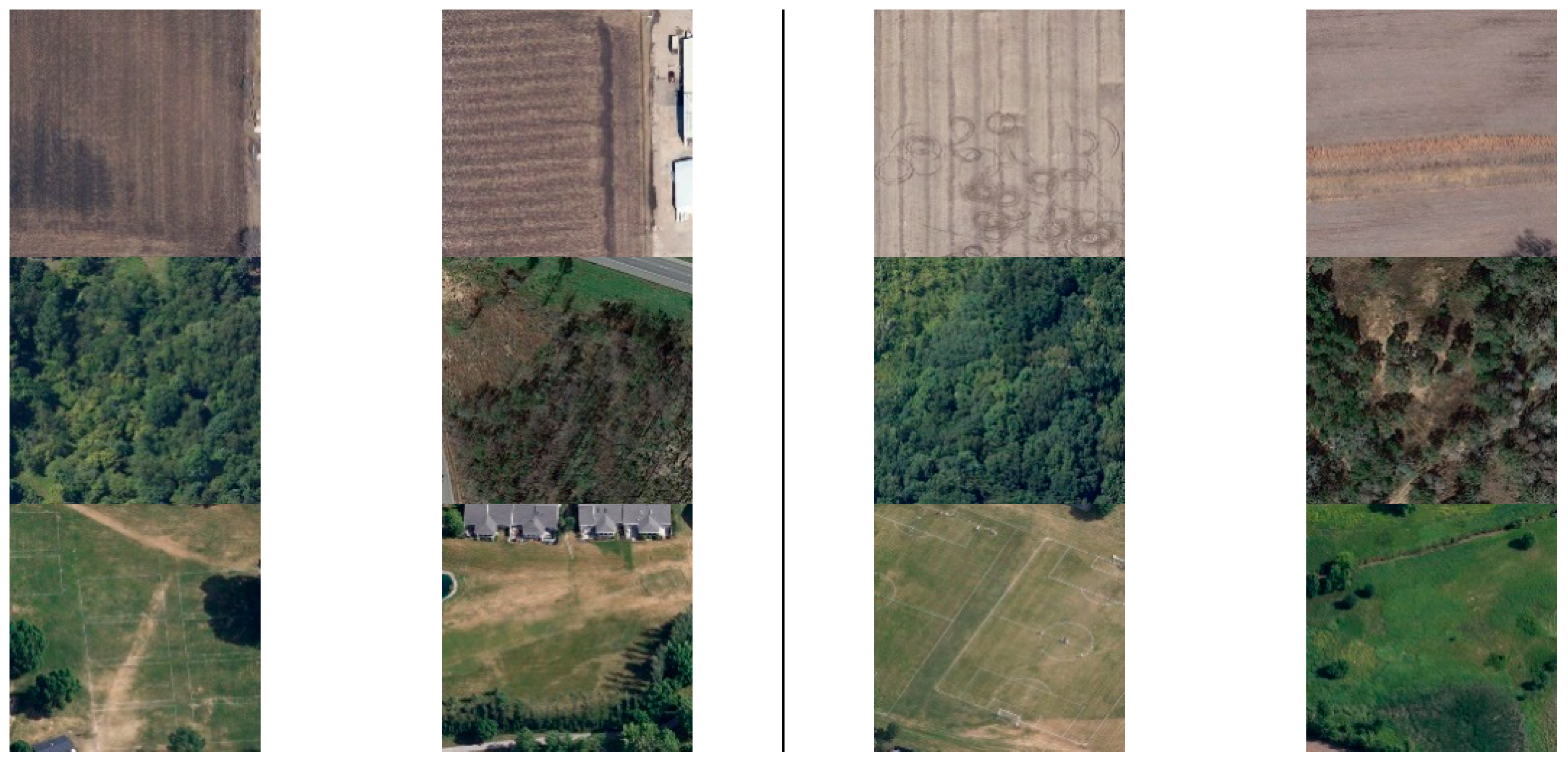
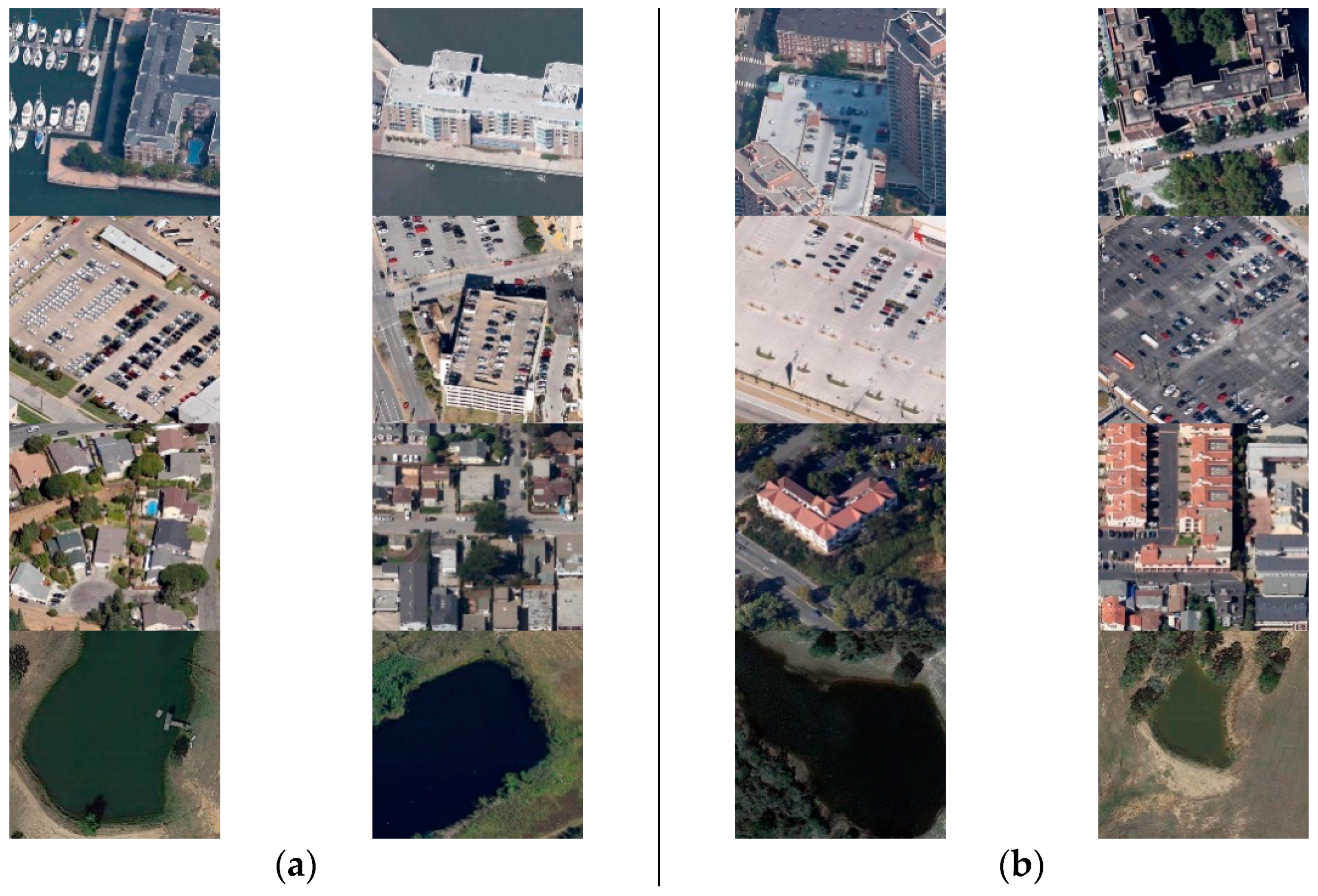
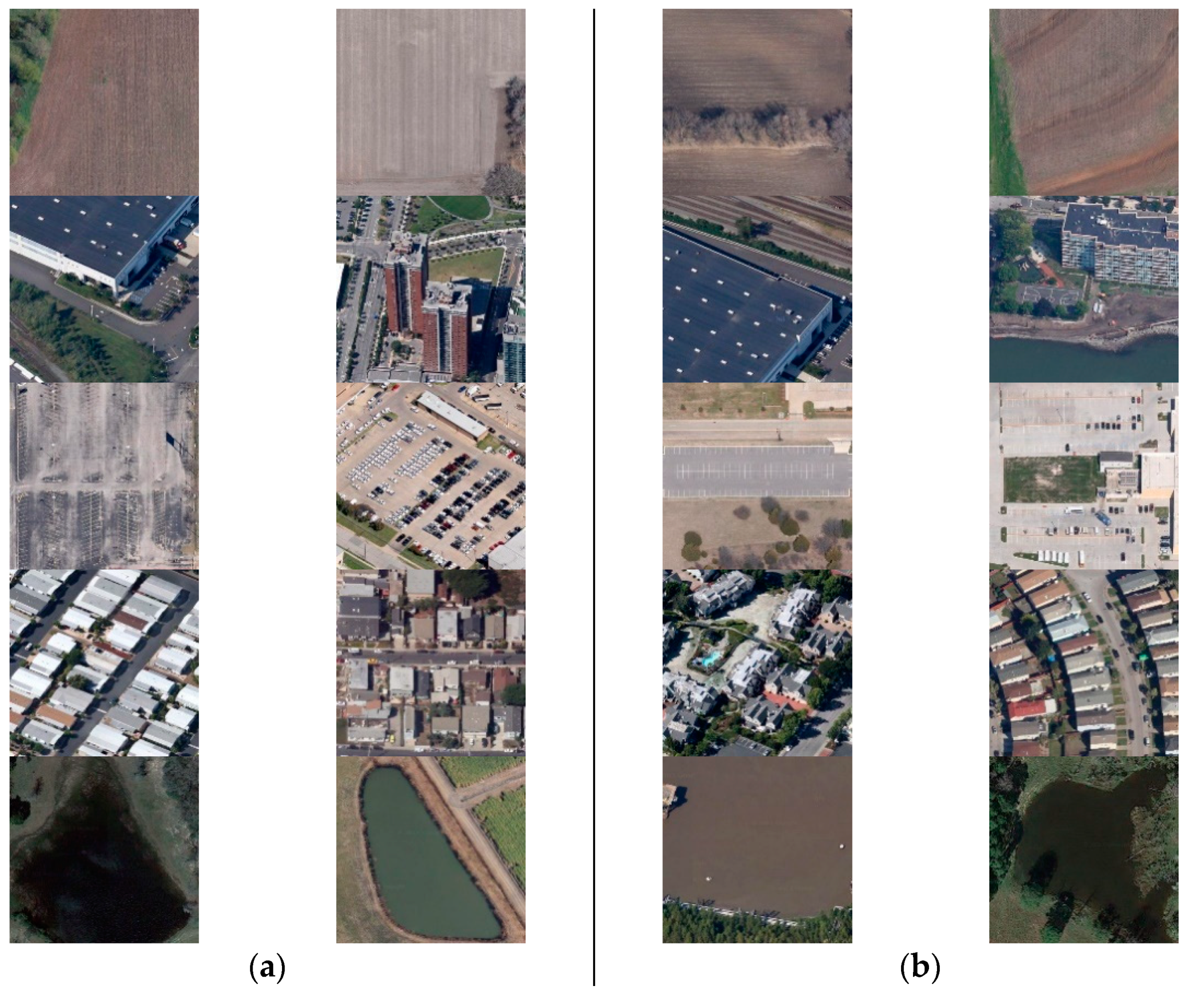
According to the above comparison, it was found that misclassification may happen when the categories between different datasets had similarities between the spectrum, contour, and texture information. To allow for a more specific and detailed visual inspection, some of the classification results of SGNAS and the models used for comparison in Section 3 are shown in Figure 14, Figure 15 and Figure 16, respectively. For example, as can be seen from the sixth row of Figure 14 and Figure 16, the proposed model can correctly classify dense and sparse residential regions scenes at the same time. The last row in Figure 15 shows that SGNAS can correctly classify the river and lack of vegetation cover or not for the experiment of SIRI-WHU→RSSCN7. Therefore, according to the results of the cross-domain experiments and the visual comparative analysis, it can be seen that the proposed model has good generalization ability, making it a good baseline network for future cross-domain research.

4.2. Comprehensive Analysis

In this section, the performance of the models that we used in the experiments are discussed from the aspect of OA. Figure 17 shows the OA values of each method on three cross-domain scenarios. SGNAS showed good performance on UCM→RSSCN7 and NWPU-RESIST45→RSSCN7, but the results for SIRI-WHU→RSSCN7 were not very good. However, the performance of the proposed SGNAS on the three cross-domain experiments was always better than other methods used for comparison. In addition, our method displayed good robustness on the three different cross-domain scenarios, as shown in Figure 17.

5. Conclusions

A spatial generalization neural search framework was proposed in this paper that applies the spatial generalization NAS to the cross-domain scene classification task of HSR remote sensing images for the first time. The framework not only includes the generalization of manually designed networks, but also has the advantages of the automatic search mechanism for traditional NAS. The network suitable for the scene classification of HSR remote sensing images can be automatically searched based on the search space level, and shows a generalization ability. A low-dimensional simple search space was designed in this paper. Based on the low-dimensional simple search space, this study generalized the search space to be extended to different tasks. The proposed framework uses the random search strategy to automatically search the model for specific HSR datasets after the search space design. The model obtained last was used for cross-domain scene classification experiments. The SIRI-WHU dataset, NWPU-RESIST45 dataset, and UCM dataset were used as training sets, and the RSSCN7 dataset was used as the test set to conduct cross-domain scene classification experiments. Experimental results demonstrate that the network obtained by the proposed SGNAS showed good generalization ability.

Author Contributions

All the authors made significant contributions to the work. Conceptualization, Q.G.; funding acquisition, Q.G.; Q.Z., Y.C. and W.T. designed the research and analyzed the results. Z.L. provided advice for the preparation of the paper. All authors have read and agreed to the published version of the manuscript.

Funding

This work was supported in part by the National Natural Science Foundation of China under grant no. 41901306; in part by the Open Research Project of The Hubei Key Laboratory of Intelligent Geo-Information Processing under grant KLIGIP-2019A02; and in part by a grant from the State Key Laboratory of Resources and Environmental Information System.

Data Availability Statement

Data associated with this research are available online. The UC Merced dataset is available for download at http://weegee.vision.ucmerced.edu/datasets/landuse.html. SIRI-WHU is available for download at for download at http://grzy.cug.edu.cn/zhuqiqi/en/index.htm. NWPU-RESIST45 dataset is available for download at http://www.escience.cn/people/JunweiHan/NWPU-RESISC45.html. RSSCN7 dataset is available for download at https://sites.google.com/site/qinzoucn/documents, all accessed on 20 July 2021.

Acknowledgments

The authors would like to thank the editor and the anonymous reviewers for their comments and suggestions.

Conflicts of Interest

The authors declare no conflict of interest.

References

  1. Zhong, Y.; Zhu, Q.; Zhang, L. Scene Classification Based on the Multifeature Fusion Probabilistic Topic Model for High Spatial Resolution Remote Sensing Imagery. IEEE Trans. Geosci. Remote Sens. 2015, 53, 6207–6222. [Google Scholar] [CrossRef]
  2. Zhu, Q.; Deng, W.; Zheng, Z.; Zhong, Y.; Guan, Q.; Lin, W.; Zhang, L.; Li, D. A Spectral-Spatial-Dependent Global Learning Framework for Insufficient and Imbalanced Hyperspectral Image Classification. IEEE Trans. Cybern. 2021. [Google Scholar] [CrossRef] [PubMed]
  3. Zhu, Q.; Zhang, Y.; Wang, L.; Zhong, Y.; Guan, Q.; Lu, X.; Zhang, L.; Li, D. A Global Context-aware and Batch-independent Network for road extraction from VHR satellite imagery. ISPRS J. Photogramm. Remote Sens. 2021, 175, 353–365. [Google Scholar] [CrossRef]
  4. Gómez-Chova, L.; Tuia, D.; Moser, G.; Camps-Valls, G. Multimodal Classification of Remote Sensing Images: A Review and Future Directions. Proc. IEEE 2015, 103, 1560–1584. [Google Scholar] [CrossRef]
  5. Blaschke, T.; Hay, G.; Kelly, M.; Lang, S.; Hofmann, P.; Addink, E.; Feitosa, R.Q.; Meer, F.D.v.d.; Werff, H.v.d.; Coillie, F.V.V.; et al. Geographic Object-Based Image Analysis Towards a new paradigm. ISPRS J. Photogramm. Remote Sens. 2014, 87, 180–191. [Google Scholar] [CrossRef] [PubMed] [Green Version]
  6. Bhaskaran, S.; Paramananda, S.; Ramnarayan, M. Per-pixel and object-oriented classification methods for mapping urban features using Ikonos satellite data. Appl. Geogr. 2010, 30, 650–665. [Google Scholar] [CrossRef]
  7. Li, D.; Tong, Q.; Li, R.; Gong, J.; Zhang, L. Some frontier scientific problems of high resolution earth observation. Chin. Sci. Geosci. 2012, 42, 805–813. [Google Scholar] [CrossRef]
  8. Bellens, R.; Gautama, S.; Martinez-Fonte, L.; Philips, W.; Chan, J.; Canters, F. Improved Classification of VHR Images of Urban Areas Using Directional Morphological Profiles. IEEE Trans. Geosci. Remote Sens. 2008, 46, 2803–2813. [Google Scholar] [CrossRef]
  9. Bratasanu, D.; Nedelcu, I.; Datcu, M. Bridging the Semantic Gap for Satellite Image Annotation and Automatic Mapping Applications. IEEE J. Sel. Top. Appl. Earth Obs. Remote Sens. 2011, 4, 193–204. [Google Scholar] [CrossRef] [Green Version]
  10. Zhu, Q.; Zhong, Y.; Zhang, L.; Li, D. Adaptive deep sparse semantic modeling framework for high spatial resolution image scene classification. IEEE Trans. Geosci. Remote Sens. 2018, 56, 6180–6195. [Google Scholar] [CrossRef]
  11. Zhao, B.; Zhong, Y.; Xia, G.-S.; Zhang, L. Dirichlet-Derived Multiple Topic Scene Classification Model for High Spatial Resolution Remote Sensing Imagery. IEEE Trans. Geosci. Remote Sens. 2016, 54, 2108–2123. [Google Scholar] [CrossRef]
  12. Xia, G.-S.; Hu, J.; Hu, F.; Shi, B.; Bai, X.; Zhong, Y.; Zhang, L.; Lu, X. AID: A Benchmark Data Set for Performance Evaluation of Aerial Scene Classification. IEEE Trans. Geosci. Remote Sens. 2017, 55, 3965–3981. [Google Scholar] [CrossRef] [Green Version]
  13. Bosch, A.; Muñoz, X.; Martí, R. Which is the best way to organize/classify images by content? Image Vis. Comput. 2007, 25, 778–791. [Google Scholar] [CrossRef]
  14. Huang, B.; Zhao, B.; Song, Y. Urban land-use mapping using a deep convolutional neural network with high spatial resolution multispectral remote sensing imagery. Remote Sens. Environ. 2018, 214, 73–86. [Google Scholar] [CrossRef]
  15. Zhong, Y.; Su, Y.; Wu, S.; Zheng, Z.; Zhao, J.; Ma, A.; Zhu, Q.; Ye, R.; Li, X.; Pellikka, P. Open-source data-driven urban land-use mapping integrating point-line-polygon semantic objects: A case study of Chinese cities. Remote Sens. Environ. 2020, 247, 111838. [Google Scholar] [CrossRef]
  16. Yang, Y.; Newsam, S. Geographic Image Retrieval Using Local Invariant Features. IEEE Trans. Geosci. Remote Sens. 2013, 51, 818–832. [Google Scholar] [CrossRef]
  17. Xia, G.-S.; Yang, W.; Delon, J.; Gousseau, Y.; Sun, H.; Maître, H. Structural high-resolution satellite image indexing. In Proceedings of the ISPRS TC VII Symposium-100 Years ISPRS, Vienna, Austria, 5–7 July 2010; pp. 298–303. [Google Scholar]
  18. Lowe, D.G. Distinctive image features from scale-invariant keypoints. Int. J. Comput. Vis. 2004, 60, 91–110. [Google Scholar] [CrossRef]
  19. Swain, M.J.; Ballard, D.H. Color indexing. Int. J. Comput. Vis. 1991, 7, 11–32. [Google Scholar] [CrossRef]
  20. Ojala, T.; Pietikainen, M.; Maenpaa, T. Multiresolution gray-scale and rotation invariant texture classification with local binary patterns. IEEE Trans. Pattern Anal. Mach. Intell. 2002, 24, 971–987. [Google Scholar] [CrossRef]
  21. Oliva, A.; Torralba, A. Modeling the Shape of the Scene: A Holistic Representation of the Spatial Envelope. Int. J. Comput. Vis. 2004, 42, 145–175. [Google Scholar] [CrossRef]
  22. Liénou, M.; Maître, H.; Datcu, M. Semantic Annotation of Satellite Images Using Latent Dirichlet Allocation. IEEE Geosci. Remote Sens. Lett. 2010, 7, 28–32. [Google Scholar] [CrossRef]
  23. Luo, W.; Li, H.; Liu, G. Automatic Annotation of Multispectral Satellite Images Using Autho’ Topic Model. IEEE Geosci. Remote Sens. Lett. 2012, 9, 634–638. [Google Scholar]
  24. Xu, S. Research on Classification of High Spatial Resolution Remote Sensing Image Based on Topic Model. Ph.D. Thesis, Shanghai Jiao Tong University, Shanghai, China, 2012. [Google Scholar]
  25. Chen, S.; Tian, Y. Pyramid of Spatial Relatons for Scene-Level Land Use Classification. IEEE Trans. Geosci. Remote Sens. 2015, 53, 1947–1957. [Google Scholar] [CrossRef]
  26. Lecun, Y.; Bengio, Y.; Hinton, G. Deep learning. Nature 2015, 521, 436. [Google Scholar] [CrossRef]
  27. Hu, F.; Xia, G.-S.; Hu, J.; Zhang, L. Transferring deep convolutional neural networks for the scene classification of high-resolution remote sensing imagery. Remote Sens. 2015, 7, 14680–14707. [Google Scholar] [CrossRef] [Green Version]
  28. Cheng, G.; Han, J.; Guo, L.; Liu, Z.; Bu, S.; Ren, J. Effective and efficient midlevel visual elements-oriented land-use classification using VHR remote sensing images. IEEE Trans. Geosci. Remote Sens. 2015, 53, 4238–4249. [Google Scholar] [CrossRef] [Green Version]
  29. Othman, E.; Bazi, Y.; Alajlan, N.; Alhichri, H.; Melgani, F. Using convolutional features and a sparse autoencoder for land-use scene classification. Int. J. Remote Sens. 2016, 37, 2149–2167. [Google Scholar] [CrossRef]
  30. Zhang, F.; Du, B.; Zhang, L. Saliency-Guided Unsupervised Feature Learning for Scene Classification. IEEE Trans. Geosci. Remote Sens. 2015, 53, 2175–2184. [Google Scholar] [CrossRef]
  31. Gu, J.; Wang, Z.; Kuen, J.; Ma, L.; Shahroudy, A.; Shuai, B.; Liu, T.; Wang, X.; Wang, G.; Cai, J. Recent advances in convolutional neural networks. Pattern Recognit. 2018, 77, 354–377. [Google Scholar] [CrossRef] [Green Version]
  32. Krizhevsky, A.; Sutskever, I.; Hinton, G.E. ImageNet classification with deep convolutional neural networks. Commun. ACM 2012, 60, 84–90. [Google Scholar] [CrossRef]
  33. Simonyan, K.; Zisserman, A. Very Deep Convolutional Networks for Large-Scale Image Recognition. arXiv 2015, arXiv:1409.1556. [Google Scholar]
  34. LeCun, Y.; Bottou, L.; Bengio, Y.; Haffner, P. Gradient-based learning applied to document recognition. Proc. IEEE 1998, 86, 2278–2324. [Google Scholar] [CrossRef] [Green Version]
  35. Wang, F.; Jiang, M.; Qian, C.; Yang, S.; Li, C.; Zhang, H.; Wang, X.; Tang, X. Residual Attention Network for Image Classification. In Proceedings of the 2017 IEEE Conference on Computer Vision and Pattern Recognition (CVPR), Honolulu, HI, USA, 21–26 July 2017; pp. 6450–6458. [Google Scholar]
  36. Hu, J.; Shen, L.; Albanie, S.; Sun, G.; Wu, E. Squeeze-and-Excitation Networks. IEEE Trans. Pattern Anal. Mach. Intell. 2020, 42, 2011–2023. [Google Scholar] [CrossRef] [PubMed] [Green Version]
  37. Woo, S.; Park, J.; Lee, J.-Y.; Kweon, I.-S. CBAM: Convolutional Block Attention Module. In Proceedings of the European conference on computer vision (ECCV), Münich, Germany, 8–14 September 2018. [Google Scholar]
  38. Iandola, F.N.; Moskewicz, M.; Ashraf, K.; Han, S.; Dally, W.; Keutzer, K. SqueezeNet: AlexNet-level accuracy with 50x fewer parameters and <1 MB model size. arXiv 2016, arXiv:1602.07360. [Google Scholar]
  39. Penatti, O.A.B.; Nogueira, K.; Santos, J.A. Do deep features generalize from everyday objects to remote sensing and aerial scenes domains? In Proceedings of the 2015 IEEE Conference on Computer Vision and Pattern Recognition Workshops (CVPRW), Boston, MA, USA, 7–12 June 2015; pp. 44–51. [Google Scholar]
  40. Zhang, P.; Gong, M.; Su, L.; Liu, J.; Li, Z. Change detection based on deep feature representation and mapping transformation for multi-spatial-resolution remote sensing images. ISPRS J. Photogramm. Remote Sens. 2016, 116, 24–41. [Google Scholar] [CrossRef]
  41. Nogueira, K.; Penatti, O.A.B.; Santos, J.A. Towards better exploiting convolutional neural networks for remote sensing scene classification. Pattern Recognit. 2017, 61, 539–556. [Google Scholar] [CrossRef] [Green Version]
  42. Cheng, G.; Han, J.; Lu, X. Remote Sensing Image Scene Classification: Benchmark and State of the Art. Proc. IEEE 2017, 105, 1865–1883. [Google Scholar] [CrossRef] [Green Version]
  43. Zhang, J.; Liu, J.; Pan, B.; Shi, Z. Domain Adaptation Based on Correlation Subspace Dynamic Distribution Alignment for Remote Sensing Image Scene Classification. IEEE Trans. Geosci. Remote Sens. 2020, 58, 7920–7930. [Google Scholar] [CrossRef]
  44. Song, S.; Yu, H.; Miao, Z.; Zhang, Q.; Lin, Y.; Wang, S. Domain adaptation for convolutional neural networks-based remote sensing scene classification. IEEE Geosci. Remote Sens. Lett. 2019, 16, 1324–1328. [Google Scholar] [CrossRef]
  45. Pan, S.J.; Yang, Q. A survey on transfer learning. IEEE Trans. Knowl. Data Eng. 2009, 22, 1345–1359. [Google Scholar] [CrossRef]
  46. Wang, Q.; Gao, J.; Li, X. Weakly supervised adversarial domain adaptation for semantic segmentation in urban scenes. IEEE Trans. Image Process. 2019, 28, 4376–4386. [Google Scholar] [CrossRef] [Green Version]
  47. Wang, J.; Zhong, Y.; Zheng, Z.; Ma, A.; Zhang, L. RSNet: The Search for Remote Sensing Deep Neural Networks in Recognition Tasks. IEEE Trans. Geosci. Remote Sens. 2021, 59, 2520–2534. [Google Scholar] [CrossRef]
  48. Zoph, B.; Vasudevan, V.; Shlens, J.; Le, Q.V. Learning Transferable Architectures for Scalable Image Recognition. In Proceedings of the 2018 IEEE/CVF Conference on Computer Vision and Pattern Recognition, Salt Lake City, UT, USA, 18–23 June 2018; pp. 8697–8710. [Google Scholar]
  49. Liu, C.; Zoph, B.; Shlens, J.; Hua, W.; Li, L.; Fei-Fei, L.; Yuille, A.; Huang, J.; Murphy, K. Progressive Neural Architecture Search. In Proceedings of the European Conference on Computer Vision (ECCV), Münich, Germany, 8–14 September 2018. [Google Scholar]
  50. Real, E.; Moore, S.; Selle, A.; Saxena, S.; Suematsu, Y.; Tan, J.; Le, Q.V.; Kurakin, A. Large-Scale Evolution of Image Classifiers. In Proceedings of the 34th International Conference on Machine Learning, Sydney, Australia, 6–11 August 2017. [Google Scholar]
  51. Miikkulainen, R.; Liang, J.; Meyerson, E.; Rawal, A.; FinkDaniel, E.; Francon, O.; Raju, B.; Shahrzad, H.; Navruzyan, A.; Duffy, N.P.; et al. Evolving Deep Neural Networks. In Artificial Intelligence in the Age of Neural Networks and Brain Computing; Academic Press: Cambridge, MA, USA, 2017; pp. 293–312. [Google Scholar]
  52. Liu, H.; Simonyan, K.; Yang, Y. DARTS: Differentiable Architecture Search. arXiv 2018, arXiv:1806.09055. [Google Scholar]
  53. Liu, C.; Chen, L.-C.; Schroff, F.; Adam, H.; Hua, W.; Yuille, A.; Fei-Fei, L. Auto-DeepLab: Hierarchical Neural Architecture Search for Semantic Image Segmentation. In Proceedings of the 2019 IEEE/CVF Conference on Computer Vision and Pattern Recognition (CVPR), Long Beach, CA, USA, 15–20 June 2019; pp. 82–92. [Google Scholar]
  54. Zoph, B.; Le, Q.V. Neural Architecture Search with Reinforcement Learning. arXiv 2016, arXiv:1611.01578. [Google Scholar]
  55. Tan, M.; Chen, B.; Pang, R.; Vasudevan, V.; Le, Q.V. MnasNet: Platform-Aware Neural Architecture Search for Mobile. In Proceedings of the 2019 IEEE/CVF Conference on Computer Vision and Pattern Recognition (CVPR), Long Beach, CA, USA, 15–20 June 2019; pp. 2815–2823. [Google Scholar]
  56. Radosavovic, I.; Kosaraju, R.P.; Girshick, R.B.; He, K.; Dollár, P. Designing Network Design Spaces. In Proceedings of the 2020 IEEE/CVF Conference on Computer Vision and Pattern Recognition (CVPR), Seattle, WA, USA, 13–19 June 2020; pp. 10425–10433. [Google Scholar]
  57. Lu, X.; Gong, T.; Zheng, X. Multisource compensation network for remote sensing cross-domain scene classification. IEEE Trans. Geosci. Remote Sens. 2019, 58, 2504–2515. [Google Scholar] [CrossRef]
  58. Li, Y.; Shi, T.; Zhang, Y.; Chen, W.; Wang, Z.; Li, H. Learning deep semantic segmentation network under multiple weakly-supervised constraints for cross-domain remote sensing image semantic segmentation. ISPRS J. Photogramm. Remote Sens. 2021, 175, 20–33. [Google Scholar] [CrossRef]
  59. Bashmal, L.; Bazi, Y.; AlHichri, H.; AlRahhal, M.M.; Ammour, N.; Alajlan, N. Siamese-GAN: Learning invariant representations for aerial vehicle image categorization. Remote Sens. 2018, 10, 351. [Google Scholar] [CrossRef] [Green Version]
  60. Othman, E.; Bazi, Y.; Melgani, F.; Alhichri, H.; Alajlan, N.; Zuair, M. Domain adaptation network for cross-scene classification. IEEE Trans. Geosci. Remote Sens. 2017, 55, 4441–4456. [Google Scholar] [CrossRef]
  61. Li, W.; Xu, Z.; Xu, D.; Dai, D.; van Gool, L. Domain generalization and adaptation using low rank exemplar SVMs. IEEE Trans. Pattern Anal. Mach. Intell. 2017, 40, 1114–1127. [Google Scholar] [CrossRef]
  62. Zhu, Q.; Zhong, Y.; Zhao, B.; Xia, G.-S.; Zhang, L. Bag-of-Visual-Words Scene Classifier with Local and Global Features for High Spatial Resolution Remote Sensing Imagery. IEEE Geosci. Remote Sens. Lett. 2016, 13, 747–751. [Google Scholar] [CrossRef]
  63. Yang, Y.; Newsam, S. Bag-of-visual-words and spatial extensions for land-use classification. In Proceedings of the 18th SIGSPATIAL international conference on advances in geographic information systems, San Jose, CA, USA, 2–5 November 2019. [Google Scholar]
  64. Zou, Q.; Ni, L.; Zhang, T.; Wang, Q. Deep Learning Based Feature Selection for Remote Sensing Scene Classification. IEEE Geosci. Remote Sens. Lett. 2015, 12, 2321–2325. [Google Scholar] [CrossRef]
  65. Liu, Z.; Lin, Y.; Cao, Y.; Hu, H.; Wei, Y.; Zhang, Z.; Lin, S.; Guo, B. Swin transformer: Hierarchical vision transformer using shifted windows. arXiv 2021, arXiv:2103.14030. [Google Scholar]
  66. Radosavovic, I.; Johnson, J.; Xie, S.; Lo, W.-Y.; Dollár, P. On network design spaces for visual recognition. In Proceedings of the IEEE/CVF International Conference on Computer Vision, Seoul, Korea, 27 October–2 November 2019; pp. 1882–1890. [Google Scholar]
  67. Bergstra, J.; Bengio, Y. Random Search for Hyper-Parameter Optimization. J. Mach. Learn. Res. 2012, 13, 281–305. [Google Scholar]
  68. He, K.; Zhang, X.; Ren, S.; Sun, J. Deep Residual Learning for Image Recognition. In Proceedings of the 2016 IEEE Conference on Computer Vision and Pattern Recognition (CVPR), Las Vegas, NV, USA, 27–30 June 2016; pp. 770–778. [Google Scholar]
  69. Pham, H.; Guan, M.; Zoph, B.; Le, Q.; Dean, J. Efficient neural architecture search via parameters sharing. In Proceedings of the International Conference on Machine Learning, Stockholm, Sweden, 10–15 July 2018; pp. 4095–4104. [Google Scholar]
Figure 1. Examples from the NWPU-RESIST45 dataset: (1) airplane, (2) airport, (3) baseball diamond, (4) basketball court, (5) beach, (6) bridge, (7) chaparral, (8) church, (9) circular farmland, (10) cloud, (11) commercial area, (12) dense residential, (13) desert, (14) forest, (15) freeway, (16) golf course, (17) ground track field, (18) harbor, (19) industrial area, (20) intersection, (21) island, (22) lake, (23) meadow, (24) medium residential, (25) mobile home park, (26) mountain, (27) overpass, (28) palace, (29) parking lot, (30) railway, (31) railway station, (32) rectangular farmland, (33) river, (34) roundabout, (35) runway, (36) sea ice, (37) ship, (38) snowberg, (39) sparse residential, (40) stadium, (41) storage tank, (42) tennis court, (43) terrace, (44) thermal power station, (45) wetland.
Remotesensing 13 03460 g001
Figure 2. Examples from the SIRI-WHU dataset: (1) farmland, (2) business quarters, (3) ports, (4) idle land, (5) industrial areas, (6) grasslands, (7) overpasses, (8) parking lots, (9) ponds, (10) residential areas, (11) rivers, (12) water.
Remotesensing 13 03460 g002
Figure 3. Examples from the UC Merced dataset: (1) agricultural, (2) airplane, (3) baseball diamond, (4) beach, (5) buildings, (6) chaparral, (7) dense residential, (8) forest, (9) freeway, (10) golf course, (11) harbor, (12) intersection, (13) medium-density residential, (14) mobile home park, (15) overpass, (16) parking lot, (17) river, (18) runway, (19) sparse residential, (20) storage tanks, (21) tennis courts.
Remotesensing 13 03460 g003
Figure 4. Examples from the RSSCN7 dataset: (1) grassland, (2) forest, (3) farmland, (4) parking lot, (5) residential region, (6) industrial region, (7) river and lake.
Remotesensing 13 03460 g004
Figure 5. Cross-domain scene classification process based on the SGNAS.
Remotesensing 13 03460 g005
Figure 6. The design process of the architecture search space in this paper.
Remotesensing 13 03460 g006
Figure 7. The basic network design of the initial search space constructed in this paper.
Remotesensing 13 03460 g007
Figure 8. The structure of residual bottleneck block. (a) Case of stride = 1, (b) Case of stride = 2.
Remotesensing 13 03460 g008
Figure 9. The process of the architecture search in this paper.
Remotesensing 13 03460 g009
Figure 10. Confusion matrix of the cross-domain scene classification results for UCM→RSSCN7.
Remotesensing 13 03460 g010
Figure 11. Confusion matrix of cross-domain scene classification results in SIRI-WHU→RSSCN7.
Remotesensing 13 03460 g011
Figure 12. Confusion matrix of the cross-domain scene classification results for NWPU-RESIST45→RSSCN7.
Remotesensing 13 03460 g012
Figure 13. Randomly sampled images from UCM, SIRI-WHU, NWPU-RESIST45, and RSSCN7 datasets. The first, second, third and fourth rows of (a) correspond to the scene classes of golf course in UCM dataset, farmland in SIRI-WHU dataset, parking lot in SIRI-WHU dataset, and farmland in the NWPU-RESIST45 dataset. The first, second, third, and fourth rows of (b) correspond to the scene classes of parking lot, industrial region, industrial region, and residential region in the RSSCN7 dataset.
Remotesensing 13 03460 g013
Figure 14. Some of the classification results of SGNAS and other models in the cross-domain scene dataset of UCM→RSSCN7. The first, second, third, fourth, fifth, sixth, and seventh rows correspond to the scene classes of farmland, forest, grassland, industrial region, parking lot, residential region, and river and lake in the RSSCN7 dataset, respectively. (a) Correctly classified images for all models. (b) Images classified correctly by SGNAS, but incorrectly classified by other models were used for comparison.
Remotesensing 13 03460 g014aRemotesensing 13 03460 g014b
Figure 15. Some of the classification results of SGNAS and other models in the cross-domain scene dataset of SIRI-WHU→RSSCN7. The first, second, third, fourth, and fifth rows correspond to the scene classes of farmland, industrial region, parking lot, residential region, and river and lake in the RSSCN7 dataset, respectively. (a) Correctly classified images for all the models. (b) Images classified correctly by SGNAS, but incorrectly classified by other models were used for comparison.
Remotesensing 13 03460 g015
Figure 16. Some of the classification results of SGNAS and other models in the cross-domain scene data set of NWPU-RESIST45→RSSCN7. The first, second, third, fourth, fifth, sixth, and seventh rows correspond to the scene classes of farmland, forest, grassland, industrial region, parking lot, residential region, and river and lake in the RSSCN7 dataset, respectively. (a) Correctly classified images for all the models. (b) Images classified correctly by SGNAS, but incorrectly classified by other models were used for comparison.
Remotesensing 13 03460 g016
Figure 17. Overall accuracy values of each model on three cross-domain scenarios.
Remotesensing 13 03460 g017
Table 1. Overall accuracy and inference time of cross-domain scene classification of different models on UCM→RSSCN7.
ModelsOA (%)Time_infer (s)
Vgg1643.7923
AlexNet44.0012
ResNet5046.719
ENAS40.8246
SGNAS59.258
Table 2. Accuracy of various scenes in cross-domain scene classification of the UCM and RSSCN7 datasets of SGNAS.
ClassAccuracy (%)
River and lake82.75
Residential region66.75
Parking lot21.25
Industrial region39.50
Grassland77.50
Forest63.75
Farmland63.25
Table 3. Overall accuracy and inference time of the cross-domain scene classification of different models for SIRI-WHU→RSSCN7.
ModelsOA (%)Time_infer (s)
Vgg1640.3037
AlexNet45.2511
ResNet5042.40142
ENAS46.95137
SGNAS53.9540
Table 4. Accuracy of various scenes in the cross-domain scene classification of the SIRI-WHU and RSSCN7 datasets of the SGNAS.
ClassAccuracy (%)
Farmland79.75
Industrial region8.25
Parking lot49.75
Residential region65.25
River and lake66.75
Table 5. Overall accuracy and inference time of the cross-domain scene classification of different models for NWPU-RESIST45→RSSCN7.
ModelsOA (%)Time_infer (s)
Vgg1641.11678
AlexNet57.8297
ResNet5060.04390
ENAS40.64860
SGNAS63.56158
Table 6. Accuracy of various scenes in the cross-domain scene classification of the NWPU-RESIST45 and RSSCN7 datasets of the SGNAS.
ClassAccuracy (%)
Farmland91.75
Forest52.50
Grassland62.25
Industrial region74.75
Parking lot76.75
Residential region20.75
River and lake60.00
Publisher’s Note: MDPI stays neutral with regard to jurisdictional claims in published maps and institutional affiliations.