Article

Moving Car Recognition and Removal for 3D Urban Modelling Using Oblique Images

1
School of Remote Sensing and Information Engineering, Wuhan University, 129 Luoyu Road, Wuhan 430079, China
2
The State Key Laboratory of Information Engineering in Surveying, Mapping and Remote Sensing, Wuhan University, 129 Luoyu Road, Wuhan 430079, China
3
Institute of Yangtze River Civilization and Archaeology, Wuhan University, 129 Luoyu Road, Wuhan 430079, China
*
Author to whom correspondence should be addressed.
Remote Sens. 2021, 13(17), 3458; https://doi.org/10.3390/rs13173458
Submission received: 14 July 2021 / Revised: 22 August 2021 / Accepted: 29 August 2021 / Published: 31 August 2021
(This article belongs to the Special Issue Urban Multi-Category Object Detection Using Aerial Images)

Abstract

:
With the progress of photogrammetry and computer vision technology, three-dimensional (3D) reconstruction using aerial oblique images has been widely applied in urban modelling and smart city applications. However, state-of-the-art image-based automatic 3D reconstruction methods cannot effectively handle the unavoidable geometric deformation and incorrect texture mapping problems caused by moving cars in a city. This paper proposes a method to address this situation and prevent the influence of moving cars on 3D modelling by recognizing moving cars and combining the recognition results with a photogrammetric 3D modelling procedure. Through car detection using a deep learning method and multiview geometry constraints, we can analyse the state of a car’s movement and apply a proper preprocessing method to the geometrically model generation and texture mapping steps of 3D reconstruction pipelines. First, we apply the traditional Mask R-CNN object detection method to detect cars from oblique images. Then, a detected car and its corresponding image patch calculated by the geometry constraints in the other view images are used to identify the moving state of the car. Finally, the geometry and texture information corresponding to the moving car will be processed according to its moving state. Experiments on three different urban datasets demonstrate that the proposed method is effective in recognizing and removing moving cars and can repair the geometric deformation and error texture mapping problems caused by moving cars. In addition, the methods proposed in this paper can be applied to eliminate other moving objects in 3D modelling applications.

1. Introduction

Three-dimensional (3D) urban modelling is an important and basic task for smart city applications such as city planning, autonomous driving, and emergency decision making [1,2]. Recently, oblique image photogrammetry has been rapidly applied in urban modelling because it can provide both geometric and texture information after automatic model reconstruction processing. The efficiency of oblique image acquisition has dramatically improved with the development of unmanned aerial vehicle (UAV) technology [3]. In addition, many exceptional algorithms for image-based 3D reconstruction have emerged [4,5,6,7,8] and have greatly increased the process efficiency and reduced the cost of 3D city digitization.
The basic assumption of multiview stereo (MVS) vision is that objects maintain a static state during image collection. However, this assumption cannot be easily satisfied in urban modelling applications because there are many moving cars during image collection. Thus, moving cars will inevitably cause errors in the modelling results, especially in the areas containing intersections. The problems caused by moving cars are summarized as follows:
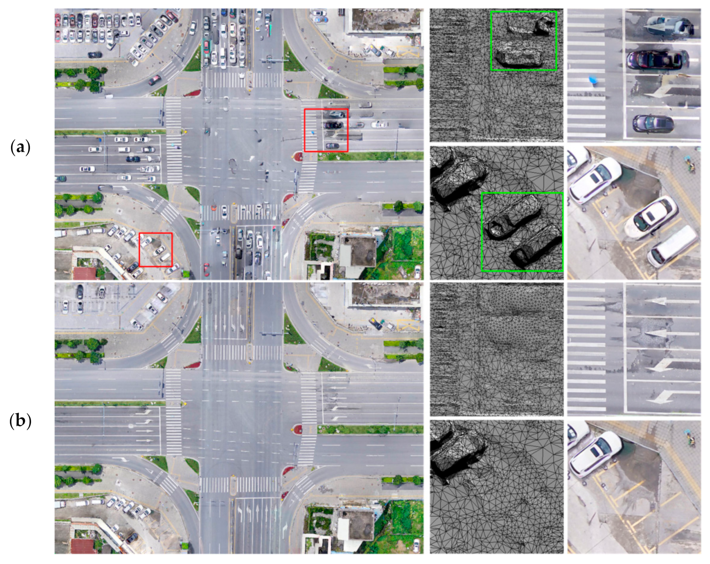
  • Geometric Deformation. If a car is stationary and then leaves during image acquisition, parts of the images will contain car information, and the other parts will not contain car information. The texture inconsistency will lead to mismatching and mesh deformations in the reconstructed 3D model. As shown in Figure 1a, the car in the red selection box was stationary and then left the region during data collection, which resulted in geometric deformations in the generated triangle mesh.
  • Error Texture Mapping. In the texture generation stage of 3D model reconstruction, moving cars will influence texture selection. If there is no pre-processing to identify moving cars, the incorrect moving-car texture information may be selected for mesh patches, resulting in texture mapping errors. As shown in Figure 1b, there are many moving cars at the intersection, and there is a large traffic flow. Due to incorrect texture selection problems caused by the moving cars in road regions, the texture of the reconstructed 3D model looks very disorganized and is quite different from the 3D model of a common road area (e.g., most of the white road marks in front of the zebra crossing are contaminated by car textures).
Figure 1. The influence of moving cars on the 3D reconstruction results, in which Figure (a) displays the mesh deformation and Figure (b) displays the texture distortion.
Remotesensing 13 03458 g001
Currently, the existing 3D reconstruction methods using multiview images cannot effectively solve the problems caused by moving cars, which are inevitable in metro cities. However, the need for realistic and accurate 3D models is still very high, especially in the applications of smart transportation, unmanned driving, etc. Therefore, manual mesh editing is a practical solution to improve model quality [9]; however, it requires considerable time and manpower. Therefore, we hope to resolve the issues by integrating moving car recognition into the 3D reconstruction pipelines to prevent the need for postprocess editing of the produced 3D models.
In this paper, we propose a moving car recognition and removal method that combines deep learning and multiview constraints. First, we use an object detection method based on depth learning to detect cars from oblique images. Subsequently, the car detection results and multiview image information are combined to recognize the moving cars. Then, the textures of the moving cars are erased from the original images, and the corresponding local deformation meshes are flattened. Finally, the car textures recognized during error detection are rejected by the random sample consensus (RANSAC) [10] method in the texture mapping step, and the texture holes are filled using available deep learning approaches.
Figure 2 shows the comparison results before and after processing the moving cars using the method proposed in this paper. The rest of this paper is organized as follows: Section 2 is a brief introduction to object detection and multiview 3D reconstruction. Section 3 elaborates on the method presented in this paper. Section 4 provides an evaluation and analysis of the experiments. The discussion is presented in the last section.

2. Related Work

2.1. Object Detection

Object detection methods mainly include three steps: region selection, feature extraction [11,12,13,14,15,16] and classification [17,18,19,20,21,22]. For example, paper [23] adopted the deformable part model (DPM [21]) classifier with a histogram of oriented gradient (HOG [14]) to detect street-view cars, and it achieved robust car detection. However, traditional object detection using rule or texture patterns has two main defects: (1) artificially designed features are subjective, usually only designed for specific detection tasks, and lack robustness to the diversity of targets; (2) when making region proposals, using a sliding window generates redundant windows, resulting in low efficiency. Thus, traditional object detection methods have low performance and high computational costs [24].
With the development of deep neural networks and the continuous improvement in GPU performance, convolutional neural networks (CNNs) have been widely used in image recognition and object detection [25]. An object detection method based on a region proposal, called R-CNN [24], was proposed to solve the problem of window redundancy in traditional methods and improve window quality while guaranteeing the recall rate. To improve detection efficiency, Fast R-CNN [26] and Faster R-CNN [27] were subsequently proposed. However, these approaches consist of two separate stages: bounding box detection and classification, and the demand for real-time detection still cannot be achieved. Therefore, a method named “you only look once” (YOLO) [28] was proposed. This method can generate a region proposal box during classification. The entire detection process has only one stage, and the speed is greatly improved. To solve the issue of inaccurate locations determined by YOLO, the single-shot detector (SSD) [29] network applies the anchor mechanism of Faster R-CNN, but SSD is not effective in detecting small objects. Similar approaches have been proposed to further improve the effectiveness [30,31,32,33] and to reach a better balance between detection accuracy and efficiency. Recently, a novel fully convolutional method named ImVoxelNet [34] was proposed, and it can obtain state-of-the-art results in car detection on KITTI [35] and nuScenes [36] benchmarks among all methods that accept RGB images.
In summary, object detection methods based on deep learning are far superior to traditional algorithms in terms of accuracy and efficiency. On the other hand, the texture patterns of cars are relatively simple and easy to detect. The reference geographic information of an image can be used to solve the scale issue of car detection because the images were collected by a drone with GPS information. Both pieces of information can improve car detection recall. In this paper, we apply the deep learning-based algorithm in reference [37] to detect car information in oblique images.

2.2. Moving Object Detection

Moving objects are unavoidable interferences in real-world scenes. In order to build clean scene models, some researchers have proposed image-based methods to detect and remove moving objects in video sequences. The related algorithms can be summarized into two types: optical flow algorithm [38] and background subtraction [39]. The general idea of the optical flow method to detect moving objects is using the concept of flow vectors in two subsequent images. The background subtraction method detects moving objects by evaluating the difference of pixel features of the current scene image against the reference background images. However, such algorithms require the camera to be fixed. Some extensions are able to handle moving cameras by registering the images against the background model [40,41]. However, this class of algorithms needs information about the appearance of the background scene, and in most cases, this assumption does not hold [42]. Moreover, other deep learning approaches to detect moving objects have also been proposed [43].
Recently, some researchers have proposed methods to detect and remove moving objects in laser data [42,44,45]. In these works, the authors exploit Dempster-Shafer Theory [46] to evaluate the occupancy of a lidar scan and discriminate points belonging to the static scene from moving ones. The differences of these works are the methods to calculate the occupancy probability, which will seriously influence the detection results. In this paper, combined with the overlap redundancy of oblique images in multiview 3D reconstruction, we introduce a method to detect moving cars using multiview constraints.

2.3. Multiview 3D Reconstruction

As shown in the green wireframe in Figure 3, multiview image-based 3D reconstruction pipelines can be divided into four stages: structure from motion (SfM) [4,8], MVS [5,47,48], surface reconstruction (mesh) [6,49] and texture mapping [7,50]. Currently, these 3D reconstruction methods can generate high-quality 3D models, but they cannot effectively solve the geometric deformation and error texture mapping problems caused by moving cars.
Researchers have proposed methods to solve these problems. Reference [7] proposed a method to remove the image patch of moving objects by texture RANSAC during the texture mapping procedure and achieved relatively good results in some situations. However, because the textures of moving objects are eliminated gradually using RANSAC iteration processing, this method will fail when there are many incorrect texture samples in the candidate images. Directly applying postprocessing to the final mesh model is another way to address geometric deformation and error texture mapping problems. Reference [9] proposed a postprocess editing method for a 3D model that is able to remove vehicles in the model by object detection, mesh flattening and image completion in the selected areas. However, this method requires manual intervention and has an image completion instability problem. We want to provide an automatic solution for the texture and geometric modelling problems caused by moving cars by integrating moving car recognition into a 3D modelling procedure.

3. Method

The method proposed in this paper combines multiview 3D reconstruction with moving car detection to achieve automatic recognition and removal of moving cars in the process of 3D model generation. The pipelines of this method are shown in Figure 3, and the green wireframe is the basic process of multiview 3D reconstruction. To solve the mesh deformation and texture error problems caused by moving cars, we integrate car detection, moving car recognition and cleaning (as shown in the red wireframe in Figure 3) into the abovementioned 3D reconstruction procedure. Each step in this method will be explained below.

3.1. Cars Detection Using Mask R-CNN

Aerial oblique image datasets captured by UAVs are the most widely used datasets for city-scale 3D modelling [51]. Compared to traditional aerial images, oblique image data have the characteristics of high spatial resolutions, a large range of scales, and large numbers. The accuracy and efficiency of an algorithm applied on oblique images should be considered when selecting the object detection method. To obtain accurate masks of cars in oblique images, we select the Mask R-CNN [37] algorithm as the network framework for car detection. Mask R-CNN adds a full convolutional network (FCN) layer to Faster R-CNN for each region of interest (ROI) and is able to detect the target object bounding box and predict the segmentation mask simultaneously. Thus, there is no need for further postprocessing of the image segmentation mask based on the bounding box. The Mask R-CNN model is shown in the green dotted box in Figure 4.
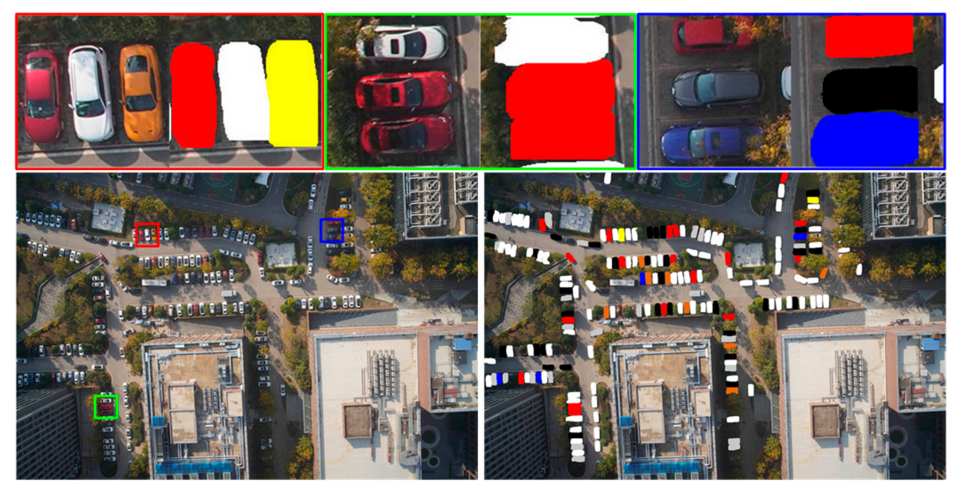
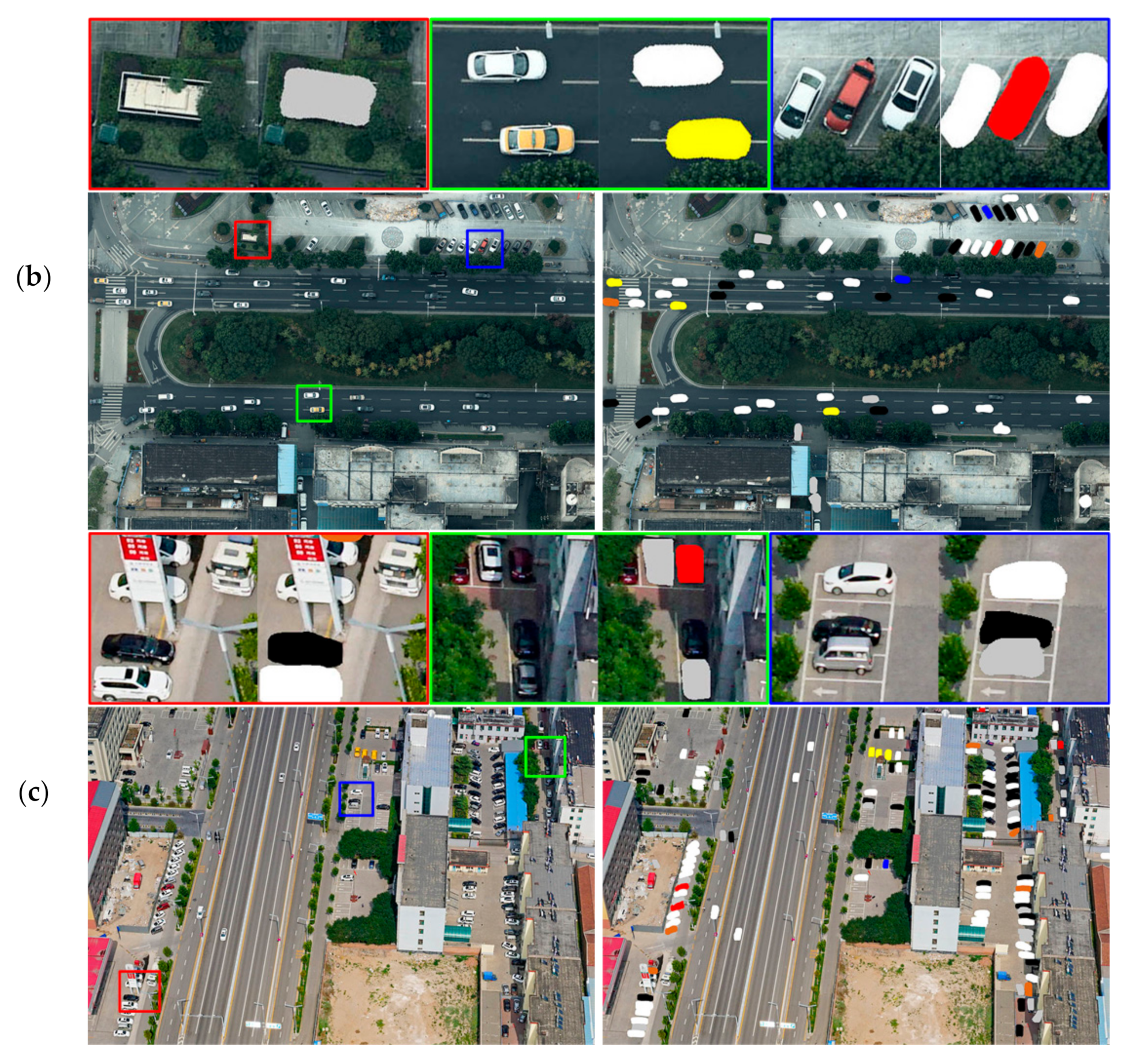
Considering that most of the vehicles in cities are cars, we divided vehicles into two types, cars and non-cars, without taking into account other vehicle types. In addition, parked-car switching (PCS), which is when a parked car leaves and another car parks in the same parking space, occurs very often in cities. We introduce a lightweight network, called MobileNet v3 [52], to classify the colour information of the detected cars and provide auxiliary reference information for PCS detection (as shown in the red dotted box of Figure 4). The colours of cars in this paper are mainly divided into white, red, yellow, blue, black, silver grey and other colours (indicated by brown in the figure). Figure 5 shows the results of the car information detected by our network model, and the masks in the figure represent the car locations and colour information.

3.2. Moving Car Recognition Based on Multiview Constraints

3.2.1. Definition of the Car Moving State (CMS)

Using the method described in Section 3.1, the location and colour information of cars can be identified in each image. However, in actual applications, the moving state of a car is more complicated than expected, and the recognition result of a car state has a serious influence on the processing strategy selection in 3D reconstruction. Therefore, to effectively solve the problems of mesh deformations and texture error mapping, we need to classify the states of the detected cars to perform a proper processing strategy according to the CMS.
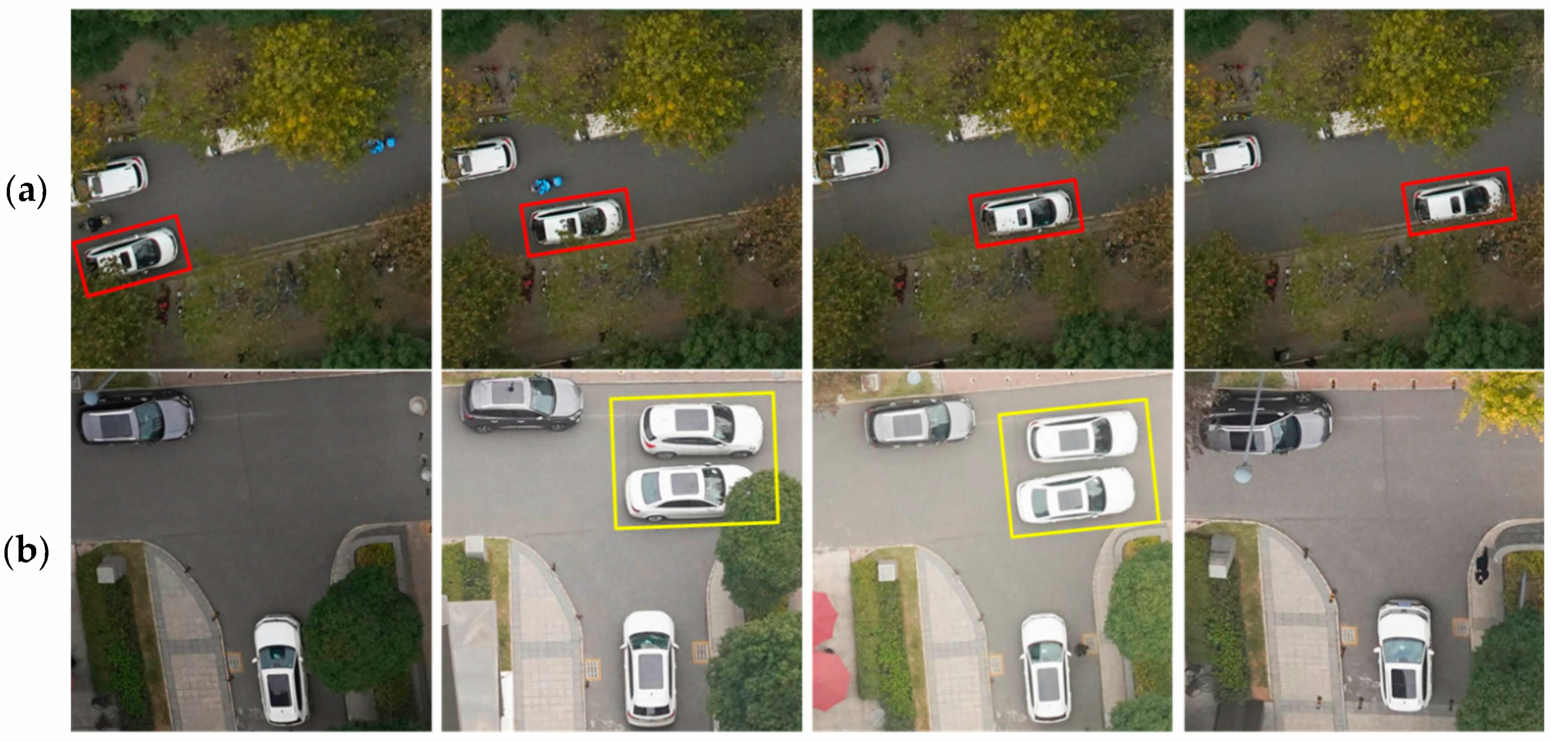
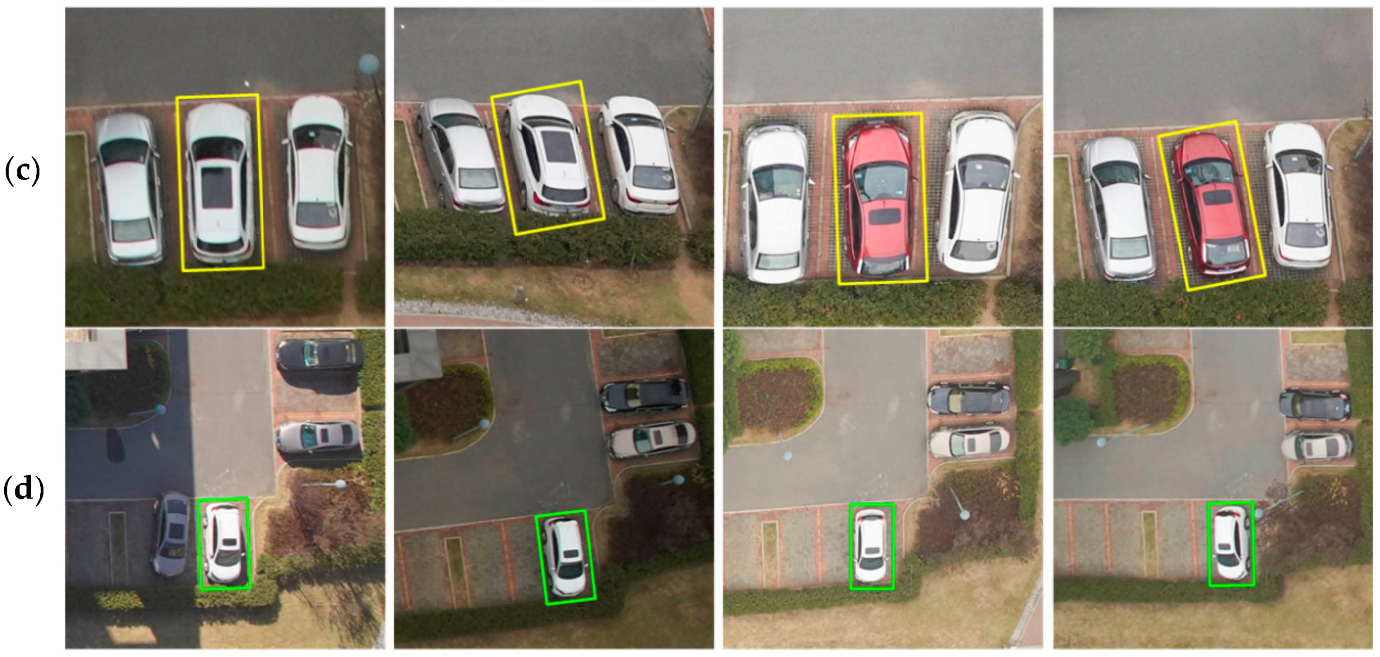
As shown in Figure 6, we divide the CMSs into the following three categories: (1) Moving: Cars that were in a driving state during image collection, as indicated by the red line box in Figure 6a; (2) Short stay: Cars that were temporarily stationary and then left during image collection, as shown in the yellow boxes in Figure 6b,c, and in Figure 6c, different cars that are stationary in the same parking region; and (3) Stationary: Cars whose parking positions never changed throughout the whole image collection process, such as the car identified by the green wireframe in Figure 6d.
According to the above definitions, for stationary cars, we do not need to perform any special processing in the 3D modelling. For a moving car, the geometric information of the car cannot be generated in the dense matching stage because it is not able to find correct correspondence pixels due to its constantly changing position in the images. Therefore, we only need to erase the texture of the moving car in the source image to prevent the problem of error texture mapping caused by the selected texture of the moving car. In the same way, for a temporarily stationary car, we not only need to erase the texture of the car in the source image but also flatten the triangle mesh of the region where the car was temporarily stationary.

3.2.2. Moving Car Recognition

  • Overview
Notably, moving cars cannot be detected by only a single image because we need to compare content between images to find “moving” information. Therefore, combined with the overlap redundancy of oblique images in multiview 3D reconstruction, we introduce a method to detect moving cars using multiview constraints. The basic principle of the method is shown in Figure 7. During image collection, if a car does not move, the corresponding texture patches of the parked car among the multiview images should be consistent. Conversely, if the texture patches of a detected car among multiview images are different, the car has moved. The green scene area in Figure 7 shows three images with different car texture patches, indicating that these cars moved. Therefore, a moving car can be recognized according to the texture differences of the detected car among multiview images.
  • Detailed Procedure for Moving Car Recognition
A triangular mesh is a data structure that is commonly used to represent 3D models created by the MVS method; however, there are multiple types of mesh structures, so in this paper, we also apply triangles as the basic computation elements. The geometric structure of an urban scene can be represented by a triangular mesh S = f i i = 1 , 2 , ... , n . We denote the captured images as I = I i i = 1 , 2 , ... , m , and the car masks detected in Section 3.1 for image I i are denoted by M a s k I i = m a s k j . The perspective projection determined by SfM of image I i is denoted by i   : R 3 R 2 , and the projection from mesh S onto the image I i is denoted by i , S   : i S S i . The specific steps for CMS recognition are shown in Algorithm 1:
  • For each image I i , sequentially remove the car mask ( m a s k j ) that has not yet been processed in M a s k I i . According to the set of triangles ( S i ) that is visible on I i , we can obtain p a t c h j by collecting the triangles whose projected positions are within the area of m a s k j (the green marked region in Figure 7).
  • Count the number of other images (denoted by n k ) that are also visible to p a t c h j but were not processed during the previous step. Count the number of detected car masks (denoted by n 1 ) that overlap with the projection region of p a t c h j in these n k images. If r a t i o 1 = n 1 / n k < δ 0 ( 0 < δ 0 < 0.08 ) , only a very small number of cars passed by p a t c h j during image collection, and m a s k j and the other n 1 car masks should be marked as moving. Then, apply this process to the next car mask m a s k j + 1 . Otherwise, go to the next step.
  • If r a t i o 1 < δ 1 ( 0.8 < δ 1 < 0.95 ) , there were cars parked in p a t c h j for a period of time during the image collection. Then, the states of these n 1 + 1 car masks should be marked as short stay, and the next car mask m a s k j + 1 should be in the processing sequence. Otherwise, the local region p a t c h j is always occupied by the car; hence, go to the next step.
  • Calculate the colour histogram of these n 1 car masks and find the largest peak value n 2 . If r a t i o 2 = n 2 / n 1 > δ 2 ( 0.75 < δ 2 < 0.9 ) , the detected corresponding texture patches of the area of p a t c h j in the multiview images are consistent and should be considered the same car. Then, the states of these n 1 + 1 masks are marked as stationary. Otherwise, the car in p a t c h j has changed, so the states of these n 1 + 1 masks are recorded as short stay. Continually apply these steps to all the unprocessed masks of cars sequentially until there are no unprocessed masks.
Algorithm 1. Car Moving State Recognition.
Input: The urban scene mesh S , car masks of each image M a s k I i
Output: The moving state of every car in each image
1. Set i = 1 , δ 0 = 0.05 , δ 1 = 0.85 , δ 2 = 0.8
2. while  i m  do
3.  Get car masks of current image I i and set j = 1
4.  while  j n i  do
5.   if the state of m a s k j in M a s k I i is unknown
6.    Count the number of other visible images ( n k ) to p a t c h j and count
the number of detected car masks ( n 1 ) that overlap with the projection region of p a t c h j
7.    if  n 1 / n k < δ 0
8.     The CMS is moving
9.    else if  n 1 / n k < δ 1
10.     The CMS is short-stay
11.    else
12.     Calculate the colour histogram of these n 1 car masks and find
      the largest peak value n 2
13.     if  n 2 / n 1 < δ 2
14.      The CMS is short-stay
15.     else
16.      The CMS is stationary
17.     end if
18.    end if
19.   end if
20.    j = j + 1
21.  end while
22.   i = i + 1
23. end while
stop

3.3. Moving Car Cleaning

3.3.1. Mesh Clean

From Section 3.2.1, we know that some regions of the 3D urban scenes will contain temporarily stationary cars during the period of image collection. If these regions containing short-stay cars were captured from multiple positions and directions by cameras during flight, some geometric errors will be introduced into the reconstructed meshes, as shown in the red marquee in Figure 1a. The deformation of the car model is very obvious, and some textures are incorrectly selected. Therefore, it is necessary to clean the triangles of the reconstructed mesh model corresponding to the patch of short-stay cars before texture mapping. Using the recognition method in Section 3.2.2, we can obtain the CMS from the given oblique images. Because the geometric structures of most parked-car regions are planar, we can directly flatten the distorted geometric meshes.

3.3.2. Texture Preprocessing

To prevent texture mapping errors caused by selecting moving cars in the texture mapping stage, it is necessary to clean the moving car textures before texture mapping. According to the recognition results in Section 3.2.2, we can erase the textures of the cars from the source oblique images that are in moving or short-stay states. However, on the one hand, some cars may not have been detected by the process in Section 3.1, and on the other hand, buses, trucks and other vehicles may not have been trained in our object detection network. Thus, the textures of these missed detection vehicles may still appear in the final 3D urban scenes. To eliminate the influence of these few unrecognized vehicle textures, we apply the RANSAC method in article [7] during texture mapping to select correct texture patches. Different from article [7], we removed most of the incorrect texture samples in the previous step, so the probability of successful missed vehicle texture cleaning is higher in our paper.
In addition, there may be different cars parked at the same place during the process of image collection, such as in the parking region in the yellow box in Figure 6c. After removing the textures of the short-stay cars, it is possible that no other textures will be available for texture mapping in these places, which will lead to a blank texture in the obtained 3D models. To prevent this situation, we use the image inpainting method in reference [53] to fill the texture holes generated by erasing the moving car textures in the candidate texture images.

4. Experiments and Discussion

4.1. Data Description

In order to cover all parts of the objects with the minimum flight time and suitable camera inclination, we collect aerial oblique images via the penta-view oblique photography platform on a DJI M600 UAV with a size of 7952 * 5304 pixels, and the ground sample distance (GSD) is 2-6 cm. We collect all experimental data in the Wuhan area, China. We select three typical regions in the urban scene to validate the proposed methods, including viaduct expressways, parking lots, and intersections with high traffic flows. In addition, aerial oblique images are captured under different weather and light conditions. The experimental data preprocessing part uses the open-source algorithms OpenMVG [54] and OpenMVS [55] on the network.

4.2. Car Detection

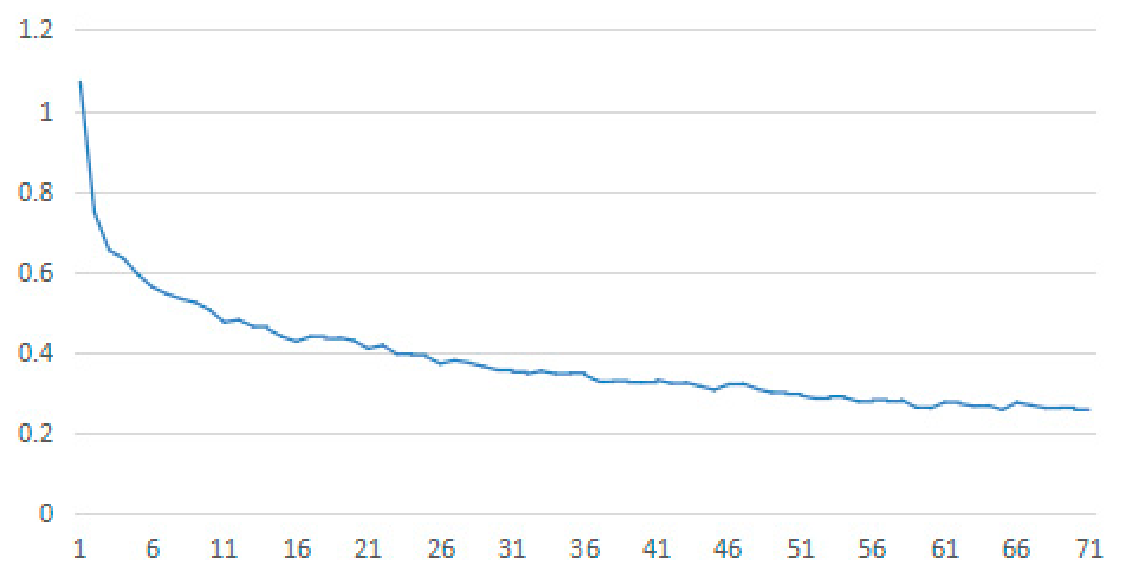
The ground truth of the training datasets for car detection was obtained manually. There are 5000 training samples with different scales, colours and shooting angles. We train the detector for 70 epochs in total and apply 1000 iterations for each epoch. With the experimental environment shown in Table 1, the training time for car detection is approximately 12 h. As depicted in Figure 8, the loss values gradually stabilize as the number of training epochs increases, indicating that the model is close to convergence. By applying the well-trained detector to the validation datasets, we obtain a mean average precision (mAP) of 92.9% for car detection and a precision of 89.7% for car colour recognition.
We also collected testing datasets with different GSDs, different shooting angles, and different lighting conditions to verify the robustness of the well-trained detector. Figure 9 shows several results of testing. Specifically, Figure 9a,b contain aerial top-view photos with GSDs of 2.5 cm, and Figure 9c contains oblique aerial images with GSDs of 3.5–6 cm. In addition, Figure 9a,c depict pictures taken under sufficient light conditions on sunny days, while Figure 9b shows the images collected on cloudy days. As shown in Table 2, the detectors perform well in the three different test scenes. However, a small number of cars are missed or falsely detected (see the red bounding boxes in Figure 9b). Furthermore, the colours of a small number of cars are incorrectly recognized. The main reasons for missed car detection are as follows:
  • Difficult samples, such as cars that are difficult to distinguish from the background, are not easy to notice. For example, a black car in a shadow is not detected (see the green box in Figure 9c).
  • It is challenging to detect cars occluded by a large region, as shown in Figure 9c in the red wireframe. Compared to the other two experimental scenes (Figure 9a,b), the third scene (Figure 9c) with a lower recall rate conforms to reality. On the one hand, there are more occlusion cases in oblique images. On the other hand, there are more shadow areas in urban scenes when light is sufficient.
In addition, we obtain different precision results for car colour recognition in the three types of scenes. (1) The test results reveal that car colour recognition precision on a cloudy day is higher than that on a sunny day. On the one hand, when the light is sufficient, some cars have reflective and overexposure problems, leading to colour recognition errors. In Figure 9a, the silver-grey car in the green wireframe is mistakenly recognized as white. On the other hand, there are more shadow areas on sunny days, which will decrease the performance of car colour recognition. As shown in the green wireframe in Figure 9c, because the quality and colour discrimination of the image in the shaded area are reduced, the white car is mistakenly identified as silver-grey. (2) We obtain a higher colour recognition precision under ortho shooting than under oblique shooting. Due to a significant variation in object scale in oblique shooting scenes, the qualities of different areas in the image are uneven, resulting in a relatively low precision for car colour recognition.

4.3. Moving Car Recognition

According to the movement state of cars defined in Section 3.2.1, we mainly select three urban scenes, including rapid urban roads, public parking areas and traffic light intersection areas, to conduct car state recognition experiments. On rapid urban roads, such as viaducts, cars are mainly moving. In public parking areas, PCS happens very often. We use the same parameters for all the recognition experiments. Specifically, we set δ 0 as 0.05, δ 1 as 0.85 and δ 2 as 0.8. Among them, δ 1 is positively related to the mAP of car detection, and δ 2 is related to the precision of car colour recognition. In our experimental results, we depict the different states of cars by mask with different colours. Red, yellow and green represent the moving state, short-stay state, and stationary state, respectively. The geometric structures of the obtained 3D models are stored using the open-source algorithm OpenMesh [56].
As shown in Figure 10, the method in Section 3.2.2 is applied to recognize car states using urban viaduct images. Figure 10e shows that all the detected cars are accurately recognized as moving because cars on rapid roads, such as urban viaducts, do not stop under normal circumstances and are always in moving states. On the other hand, Figure 10c also shows that among the textures in the multiview images of the red frame area in Figure 10a, most do not have corresponding car information. Therefore, according to the recognition rules in Section 3.2.2, the car corresponding to the local scene area is a moving car, and its texture in Figure 10a should be erased.
We select a small parking lot in front of an office building for the public parking lot urban scenes, as pictured in Figure 11. It can be seen from the recognition results of the car state in Figure 11c that most of the cars in the parking lot area never moved, and only a small number of cars were temporarily stationary. Table 3 shows the statistical results using the method in Section 3.2.2 for some of the car areas selected in Figure 11a. Table 3 reveals that the value of r a t i o 1 or r a t i o 2 is relatively low for short-stay cars. Moreover, the value r a t i o 1 of the yellow box is relatively high, while the value r a t i o 2 is relatively low, indicating that different cars were located in the same parking region and that this is a case of PCS.
Furthermore, the geometric mesh of the scene in Figure 11b helps to further verify the recognition results in Figure 11c. For the regions where cars have stayed (see the green and yellow masked parts in Figure 11c), the geometric structures of the cars at the corresponding positions in Figure 11b have been reconstructed. Conversely, if the geometric structure is not reconstructed, as shown in the red box in Figure 11a,b, the car is in a moving state, and its value n1 is relatively small. In the same way, we can also learn from the 3D car models in the yellow boxes in Figure 11b that there are cars parked on these unoccupied regions in Figure 11a during other periods of image acquisition, so they are in the short-stay state. In addition, it can be seen from the green-box areas in Figure 11d that the triangle meshes of the short-stay regions are flat.
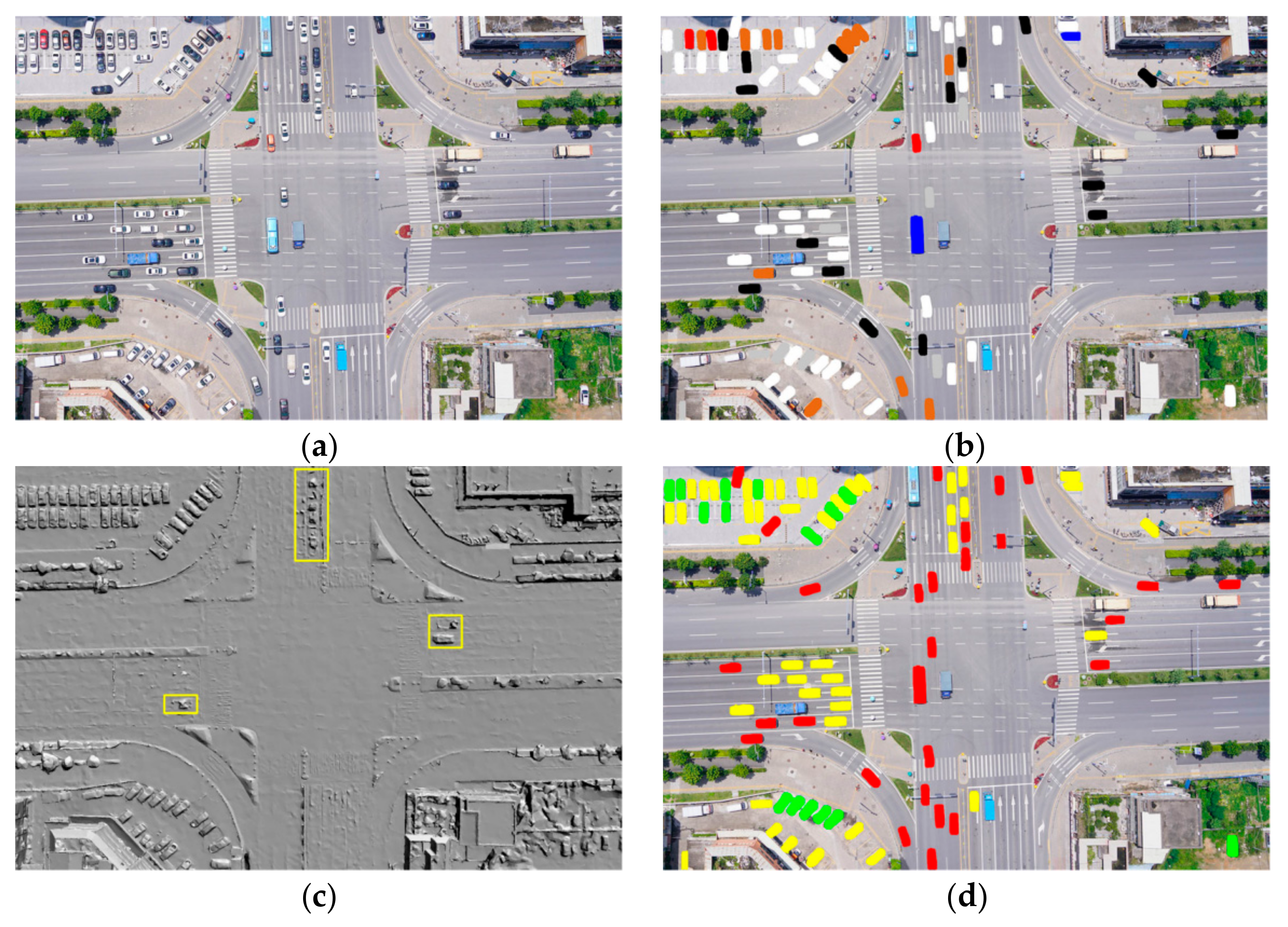
To further verify the effectiveness of the proposed method, we select an intersection area (see Figure 12a) that has a heavy traffic flow and contains various cars in the three different states defined for the experiments. Figure 12b shows the results of car detection in Figure 12a, from which it can be seen that the cars in the scene are well detected. Figure 12d shows the state recognition results of the cars detected in Figure 12b. Figure 12d reveals that the cars on the road are mostly in moving states, while the cars waiting for the traffic lights are likely in the short-stay state. The geometric deformation results of the car models in the yellow boxes in Figure 12c also explain this result. PCS frequently occurs in parking lot spaces (see the top left of Figure 12a). However, unlike Figure 11, more PCS cases occur in this region, where the yellow masks are more than the green masks. Parked cars change more frequently since the parking lot in Figure 12a is in front of a mall.

4.4. Moving Car Cleaning

Once the states of the cars are recognized, the textures of the moving cars can be erased effectively from the oblique images. Additionally, the geometric deformation caused by the temporarily stationary cars can be easily repaired. In this section, we carry out comparative tests based on the experimental results in Section 4.3 to validate the effectiveness of our method in removing moving cars during 3D reconstruction.
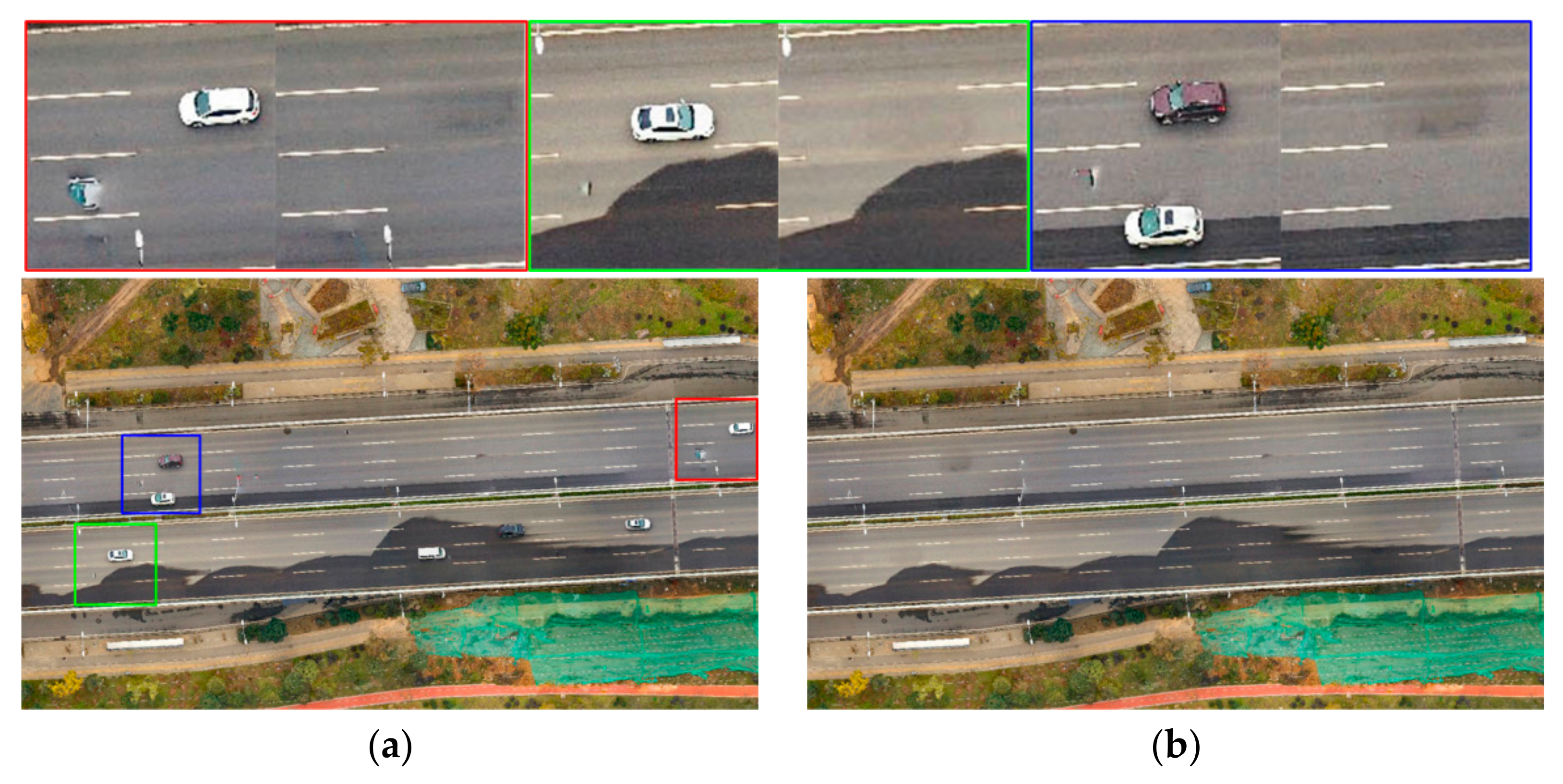
Figure 13 depicts the comparison results of moving car removal from the urban viaduct scene in Figure 10. Specifically, we obtain the 3D scene in Figure 13a using traditional 3D reconstruction pipelines. In addition, we reconstruct the 3D model in Figure 13b via the proposed method in this paper. From the comparison results, the method proposed in this article can effectively remove the textures of all moving cars from the viaduct pavement, and the 3D scene of the whole viaduct road looks clean. Moreover, the information about stationary cars is preserved completely.
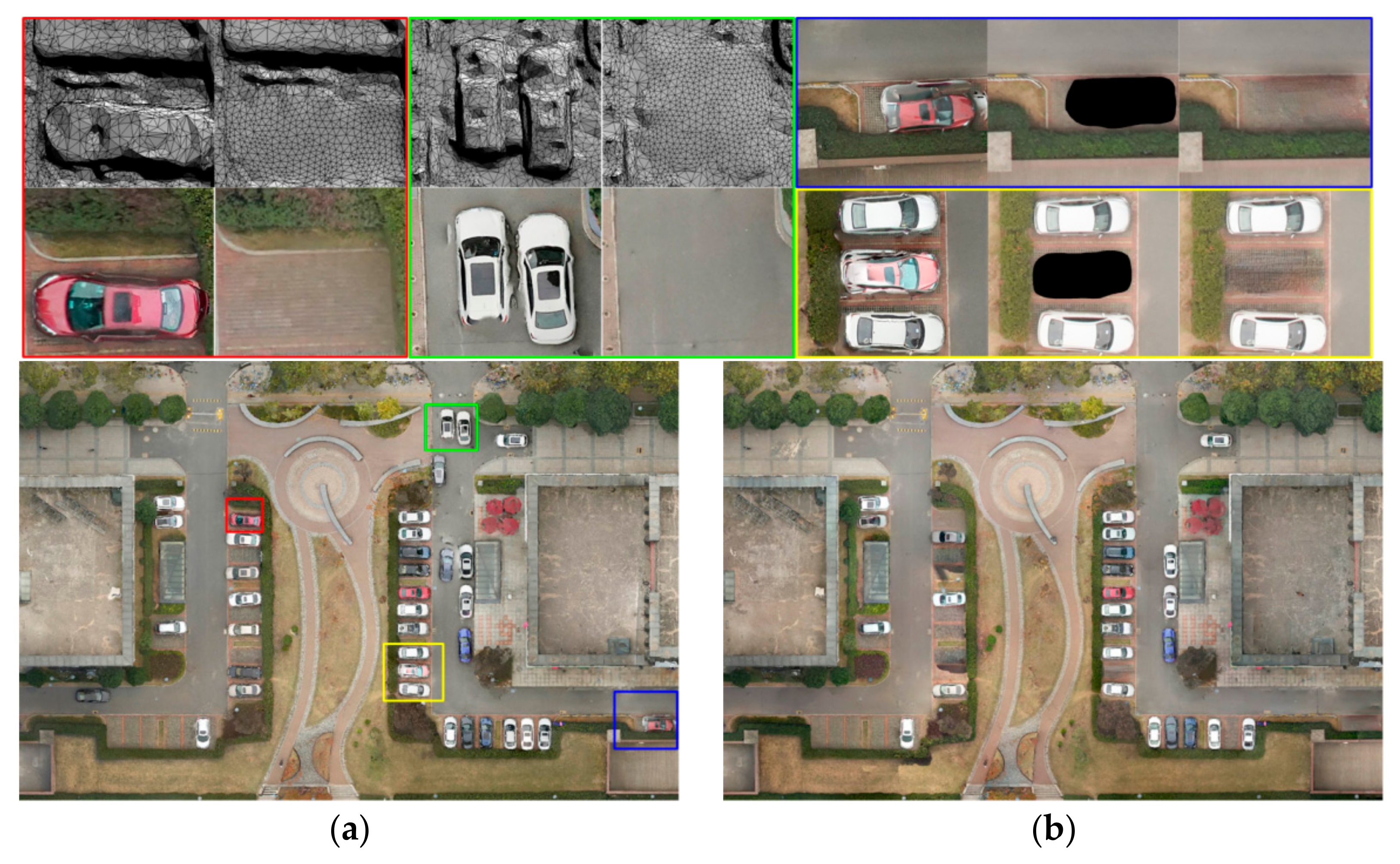
Figure 14 shows the experimental results of moving car removal from the parking lot scene in Figure 11. Two cases (the red and green box regions) were selected from Figure 14a,b, respectively, and demonstrate that our proposed method can better handle the geometry and texture of areas where cars were temporarily stationary. In addition, the parking spaces highlighted by the blue and yellow boxes in Figure 14 are occupied by different cars during the whole process of image acquisition. Therefore, for this kind of region, we need to fill in the texture voids in the images according to the rules in Section 3.3.2. Taking advantage of the algorithm in [53], we obtain a satisfactory region filling result. The comparison results are shown in the blue and yellow boxes in Figure 14.
Figure 15 shows the results of moving car removal from the intersection area in Figure 12. Similarly, we reconstruct the 3D scenes in Figure 15a,b using the traditional pipeline and the proposed method, respectively. The entire 3D scene in Figure 15a undoubtedly looks disorganised due to the moving cars. Compared to the results in Figure 15a, we obtain a more accurate and realistic 3D intersection scene after mesh cleaning and texture preprocessing, especially for typical road areas. All the moving vehicles on the road, including undetected buses and vans, are effectively removed, indicating that the proposed method is robust.

5. Conclusions

This paper proposes a method for moving car recognition and removal that combines deep learning and multiview constraints. Our method mainly includes three steps: car detection, moving car recognition and cleaning. The main contribution of this paper is to integrate object detection into 3D reconstruction pipelines to eliminate the geometric and texture problems caused by moving cars. Compared with the traditional 3D reconstruction method based on multiview images, the experimental results indicate that the proposed method can effectively moderate geometric deformations and texture distortions caused by moving cars in 3D urban scenes. In addition, the method in this paper has a high degree of automation, which can distinctly reduce the workload of manual postprocessing to repair 3D scene models, thereby improving the production efficiency of urban 3D scene modelling.
However, the method proposed in this paper is limited by the following issues, which provide insights for developing future works. (1) We have not yet considered other types of vehicles due to a lack of training samples in our object recognition experiments. Unfortunately, our training samples only contain cars, so other vehicles, such as motorcycles, buses, and trucks, are easily ignored during detection. (2) We only take advantage of colour information to distinguish the PCS cases. This method for similarity detection is too limited to be robust. Therefore, we will further explore this area in future work.

Author Contributions

Conceptualization, F.Z., X.H. and Y.G.; data curation, X.H.; formal analysis, C.Y., F.Z., Y.G., X.H., L.L. and Z.M.; funding acquisition, F.Z.; methodology, C.Y.; writing—original draft, C.Y.; writing—review and editing, C.Y., F.Z., X.H., L.L. and Z.M. All authors have read and agreed to the published version of the manuscript.

Funding

This research was funded by the National Key R&D Program of China No. 2020YFC1523003 and No. 2020YFC1522703.

Data Availability Statement

The data presented in this study are available on request from the corresponding author.

Acknowledgments

The authors would like to thank the researchers who have provided the opensource algorithms, which have been extremely helpful to the research in this paper.

Conflicts of Interest

The authors declare no conflict of interest.

References

  1. Yang, B.; Dong, Z.; Liu, Y.; Liang, F.; Wang, Y. Computing multiple aggregation levels and contextual features for road facilities recognition using mobile laser scanning data. ISPRS J. Photogramm. Remote Sens. 2017, 126, 180–194. [Google Scholar] [CrossRef]
  2. Toschi, I.; Ramos, M.M.; Nocerino, E.; Menna, F.; Remondino, F.; Moe, K.; Poli, D.; Legat, K.; Fassi, F. Oblique photogrammetry supporting 3D urban reconstruction of complex scenarios. ISPRS-Int. Arch. Photogramm. Remote Sens. Spat. Inf. Sci. 2017, XLII-1/W1, 519–526. [Google Scholar] [CrossRef] [Green Version]
  3. Jiang, S.; Jiang, W.S.; Huang, W.; Yang, L. UAV-Based Oblique Photogrammetry for Outdoor Data Acquisition and Offsite Visual Inspection of Transmission Line. Remote Sens. 2017, 9, 278. [Google Scholar] [CrossRef] [Green Version]
  4. Moulon, P.; Monasse, P.; Marlet, R. Global fusion of relative motions for robust, accurate and scalable structure from motion. In Proceedings of the IEEE International Conference on Computer Vision, Sydney, Australia, 3–6 December 2013; pp. 3248–3255. [Google Scholar] [CrossRef] [Green Version]
  5. Han, Y.L.; Liu, W.; Huang, X.; Wang, S.G.; Qin, R.J. Stereo Dense Image Matching by Adaptive Fusion of Multiple-Window Matching Results. Remote Sens. 2020, 12, 3138. [Google Scholar] [CrossRef]
  6. Xu, Z.Q.; Xu, C.; Hu, J.; Meng, Z.P. Robust resistance to noise and outliers: Screened Poisson Surface Reconstruction using adaptive kernel density estimation. Comput. Graph. 2021, 97, 19–27. [Google Scholar] [CrossRef]
  7. Waechter, M.; Moehrle, N.; Goesele, M. Let There Be Color! Large-Scale Texturing of 3D Reconstructions. In Computer Vision—ECCV 2014. ECCV 2014. Lecture Notes in Computer Science; Springer: Cham, Switzerland, 2014; Volume 869, pp. 836–850. [Google Scholar] [CrossRef]
  8. Verykokou, S. Georeferencing Procedures for Oblique Aerial Images. Ph.D. Thesis, National Technical University of Athens, Athens, Greece, 2020. [Google Scholar]
  9. Zhu, Q.; Shang, Q.S.; Hu, H.; Yu, H.J.; Zhong, R.F. Structure-aware completion of photogrammetric meshes in urban road environment. ISPRS J. Photogramm. Remote Sens. 2021, 175, 56–70. [Google Scholar] [CrossRef]
  10. Fischler, M.A.; Bolles, R.C. Random sample consensus: A paradigm for model fitting with applications to image analysis and automated cartography. Commun. ACM 1981, 24, 381–395. [Google Scholar] [CrossRef]
  11. Rublee, E.; Rabaud, V.; Konolige, K.; Bradski, G. ORB: An efficient alternative to SIFT or SURF. In Proceedings of the IEEE International Conference on Computer Vision, Barcelona, Spain, 6–13 November 2011. [Google Scholar] [CrossRef]
  12. Lowe, D.G. Distinctive Image Features from Scale-invariant Keypoints. Int. J. Comput. Vis. 2004, 60, 91–110. [Google Scholar] [CrossRef]
  13. Papageorgiou, C.P.; Oren, M.; Poggio, T. A General Framework for Object Detection. In Proceedings of the Sixth International Conference on Computer Vision, Bombay, India, 7 January 1998; pp. 555–562. [Google Scholar] [CrossRef] [Green Version]
  14. Dalal, N.; Triggs, B. Histograms of Oriented Gradients for Human Detection. In Proceedings of the IEEE Computer Society Conference on Computer Vision and Pattern Recognition, San Diego, CA, USA, 20–25 June 2005; Volume 1, pp. 886–893. [Google Scholar] [CrossRef] [Green Version]
  15. Ojala, T.; Pietikäinen, M.; Mäenpää, T. Gray Scale and Rotation Invariant Texture Classification with Local Binary Patterns. In Computer Vision—ECCV 2000. ECCV 2000. Lecture Notes in Computer Science; Springer: Berlin/Heidelberg, Germany, 2000; Volume 1842, pp. 404–420. [Google Scholar] [CrossRef] [Green Version]
  16. Bay, H.; Ess, A.; Tuytelaars, T.; Gool, L.V. Speeded-Up Robust Features (SURF). Comput. Vis. Image Underst. 2008, 110, 346–359. [Google Scholar] [CrossRef]
  17. Quinlan, J.R. Induction of Decision Trees. Mach. Learn. 1986, 1, 81–106. [Google Scholar] [CrossRef] [Green Version]
  18. Kononenko, I. Semi-naive Bayesian Classifier. In Lecture Notes in Computer Science; Springer: Berlin/Heidelberg, Germany, 1991; Volume 482, pp. 206–219. [Google Scholar] [CrossRef]
  19. Suykens, J.A.K.; Lukas, L.; Dooren, V.P.; Moor, D.B.; Vandewalle, J. Least Squares Support Vector Machine Classifiers: A Large Scale Algorithm. In Proceedings of the European Conference on Circuit Theory and Design, Stresa, Italy, 29 August–2 September 1999; pp. 839–842. [Google Scholar] [CrossRef]
  20. Freund, Y.; Schapire, R.E. A Decision-Theoretic Generalization of On-Line Learning and an Application to Boosting. J. Comput. Syst. Sci. 1999, 55, 119–139. [Google Scholar] [CrossRef] [Green Version]
  21. Felzenszwalb, P.F.; Girshick, R.B.; McAllester, D.; Ramanan, D. Object Detection with Discriminatively Trained Part-based Models. IEEE Trans. Pattern Anal. Mach. Intell. 2010, 32, 1627–1645. [Google Scholar] [CrossRef] [Green Version]
  22. Breiman, L. Random Forest. Mach. Learn. 2001, 45, 5–32. [Google Scholar] [CrossRef] [Green Version]
  23. Chu, W.T.; Chao, Y.C.; Chang, Y.S. Street sweeper: Detecting and removing cars in street view images. Multimed. Tools Appl. 2015, 74, 10965–10988. [Google Scholar] [CrossRef]
  24. Girshick, R.; Donahue, J.; Darrell, T.; Malik, J. Rich feature hierarchies for accurate object detection and semantic segmentation. In Proceedings of the IEEE Conference on Computer Vision and Pattern Recognition, Columbus, OH, USA, 24–27 June 2014; pp. 580–587. [Google Scholar] [CrossRef] [Green Version]
  25. Simonyan, K.; Zisserman, A. Very deep convolutional networks for large-scale image recognition. In Proceedings of the 3rd International Conference on Learning Representations, San Diego, CA, USA, 7–9 May 2015. [Google Scholar]
  26. Girshick, R. Fast R-CNN. In Proceedings of the IEEE International Conference on Computer Vision, Las Condes, Chile, 11–18 December 2015; pp. 1440–1448. [Google Scholar] [CrossRef]
  27. Ren, S.Q.; He, K.M.; Girshick, R.B.; Sun, J. Faster r-cnn: Towards real-time object detection with region proposal networks. IEEE Trans. Pattern Anal. Mach. Intell. 2017, 39, 1137–1149. [Google Scholar] [CrossRef] [Green Version]
  28. Redmon, J.; Divvala, S.K.; Girshick, R.B.; Farhadi, A. You Only Look Once: Unified, Real-Time Object Detection. In Proceedings of the IEEE Conference on Computer Vision and Pattern Recognition, Las Vegas, NV, USA, 27–30 June 2016; pp. 779–788. [Google Scholar] [CrossRef] [Green Version]
  29. Liu, W.; Anguelov, D.; Erhan, D.; Szegedy, C.; Reed, S.; Fu, C.Y.; Berg, A.C. SSD: Single Shot MultiBox Detector. In Proceedings of the European Conference on Computer Vision, Amsterdam, The Netherlands, 11–14 October 2016; Volume 9905, pp. 21–37. [Google Scholar] [CrossRef] [Green Version]
  30. Redmon, J.; Farhadi, A. YOLO9000: Better, Faster, Stronger. In Proceedings of the IEEE Conference on Computer Vision and Pattern Recognition, Honolulu, HI, USA, 21–26 July 2017; pp. 6517–6525. [Google Scholar] [CrossRef] [Green Version]
  31. Redmon, J.; Farhadi, A. Yolov3: An Incremental Improvement. arXiv 2018, arXiv:1804.02767. [Google Scholar]
  32. Bochkovskiy, A.; Wang, C.Y.; Liao, H.Y.M. YOLOv4: Optimal Speed and Accuracy of Object Detection. arXiv 2020, arXiv:2004.10934. [Google Scholar]
  33. YOLOv5. Available online: https://github.com/ultralytics/yolov5 (accessed on 10 July 2021).
  34. Rukhovich, D.; Vorontsova, A.; Konushin, A. ImVoxelNet: Image to Voxels Projection for Monocular and Multi-View General-Purpose 3D Object Detection. arXiv 2021, arXiv:2106.01178. [Google Scholar]
  35. Geiger, A.; Lenz, P.; Urtasun, R. Are we ready for autonomous driving? The kitti vision benchmark suite. In Proceedings of the 2012 IEEE Conference on Computer Vision and Pattern Recognition, Providence, RI, USA, 16–21 June 2012; pp. 3354–3361. [Google Scholar] [CrossRef]
  36. Caesar, H.; Bankiti, V.; Lang, A.H.; Vora, S.; Liong, V.E.; Xu, Q.; Krishnan, A.; Pan, Y.; Baldan, G.; Beijbom, O. nuscenes: A multimodal dataset for autonomous driving. In Proceedings of the IEEE/CVF Conference on Computer Vision and Pattern Recognition, Seattle, WA, USA, 13–19 June 2020; pp. 11618–11628. [Google Scholar] [CrossRef]
  37. He, K.; Gkioxari, G.; Dollár, P.; Girshick, R. Mask R-CNN. IEEE Trans. Pattern Anal. Mach. Intell. 2017, 42, 386–397. [Google Scholar] [CrossRef] [PubMed]
  38. Agarwal, A.; Gupta, S.; Singh, D.K. Review of optical flow technique for moving object detection. In Proceedings of the 2016 2nd International Conference on Contemporary Computing and Informatics (IC3I), Greater Noida, India, 14–17 December 2017; pp. 409–413. [Google Scholar]
  39. Barnich, O.; Droogenbroeck, M.V. ViBe: A universal background subtraction algorithm for video sequences. IEEE Trans. Image Process. 2011, 20, 1709–1724. [Google Scholar] [CrossRef] [Green Version]
  40. Romanoni, A.; Matteucci, M.; Sorrenti, D.G. Background subtraction by combining temporal and spatio-temporal histograms in the presence of camera movement. Mach. Vis. Appl. 2014, 25, 1573–1584. [Google Scholar] [CrossRef] [Green Version]
  41. Kim, S.W.; Yun, K.; Yi, K.M.; Kim, S.J.; Choi, J.Y. Detection of moving objects with a moving camera using non-panoramic background model. Mach. Vis. Appl. 2013, 24, 1015–1028. [Google Scholar] [CrossRef]
  42. Postica, G.; Romanoni, A.; Matteucci, M. Robust Moving Objects Detection in Lidar Data Exploiting Visual Cues. In Proceedings of the 2016 IEEE/RSJ International Conference on Intelligent Robots and Systems, Daejeon, Korea, 9–14 October 2016; pp. 1093–1098. [Google Scholar] [CrossRef] [Green Version]
  43. Lin, T.H.; Wang, C.C. Deep learning of spatio-temporal features with geometric-based moving point detection for motion segmentation. In Proceedings of the 2014 IEEE International Conference on Robotics and Automation, Hong Kong, China, 31 May–7 June 2014; pp. 3058–3065. [Google Scholar] [CrossRef]
  44. Vallet, B.; Xiao, W.; Bredif, M. Extracting mobile objects in images using a velodyne lidar point cloud. ISPRS Ann. Photogramm. Remote Sens. Spat. Inf. Sci. 2015, 1, 247–253. [Google Scholar] [CrossRef] [Green Version]
  45. Hara, Y.; Tomono, M. Moving object removal and surface mesh mapping for path planning on 3D terrain. Adv. Robot. 2020, 34, 375–387. [Google Scholar] [CrossRef]
  46. Bundy, A.; Wallen, L. Dempster-Shafer Theory; Springer: Berlin/Heidelberg, Germany, 1984. [Google Scholar]
  47. Yan, L.; Fei, L.; Chen, C.H.; Ye, Z.Y.; Zhu, R.X. A Multi-View Dense Image Matching Method for High-Resolution Aerial Imagery Based on a Graph Network. Remote Sens. 2016, 8, 799. [Google Scholar] [CrossRef] [Green Version]
  48. Bleyer, M.; Rhemann, C.; Rother, C. PatchMatch Stereo-Stereo Matching with Slanted Support Windows. In Proceedings of the British Machine Vision Conference, Dundee, UK, 29 August–2 September 2011; pp. 1–11. [Google Scholar] [CrossRef] [Green Version]
  49. Pan, H.L.; Guan, T.; Luo, K.Y.; Luo, Y.W.; Yu, J.Q. A visibility-based surface reconstruction method on the GPU. Comput. Aided Geom. Des. 2021, 84, 101956. [Google Scholar] [CrossRef]
  50. Bi, S.; Kalantari, N.K.; Ramamoorthi, R. Patch-based optimization for image-based texture mapping. ACM Trans. 2017, 36, 106. [Google Scholar] [CrossRef]
  51. Google Earth. Available online: https://www.google.com/earth/ (accessed on 10 July 2021).
  52. Howard, A.; Sandler, M.; Chen, B.; Wang, W.J.; Chen, L.C.; Tan, M.X.; Chu, G.; Vasudevan, V.; Zhu, Y.; Pang, R.; et al. Searching for MobileNetV3. In Proceedings of the International Conference on Computer Vision, Seoul, Korea, 27 October–2 November 2019; pp. 1314–1324. [Google Scholar] [CrossRef]
  53. Yu, J.H.; Lin, Z.; Yang, J.M.; Shen, X.H.; Lu, X.; Huang, T. Free-Form Image Inpainting with Gated Convolution. In Proceedings of the International Conference on Computer Vision, Seoul, Korea, 27 October–2 November 2019; pp. 4470–4479. [Google Scholar] [CrossRef] [Green Version]
  54. OpenMVG. Available online: https://github.com/openMVG/openMVG (accessed on 10 July 2021).
  55. OpenMVS. Available online: https://github.com/cdcseacave/openMVS (accessed on 10 July 2021).
  56. OpenMesh. Available online: https://www.graphics.rwth-aachen.de/software/openmesh/ (accessed on 10 July 2021).
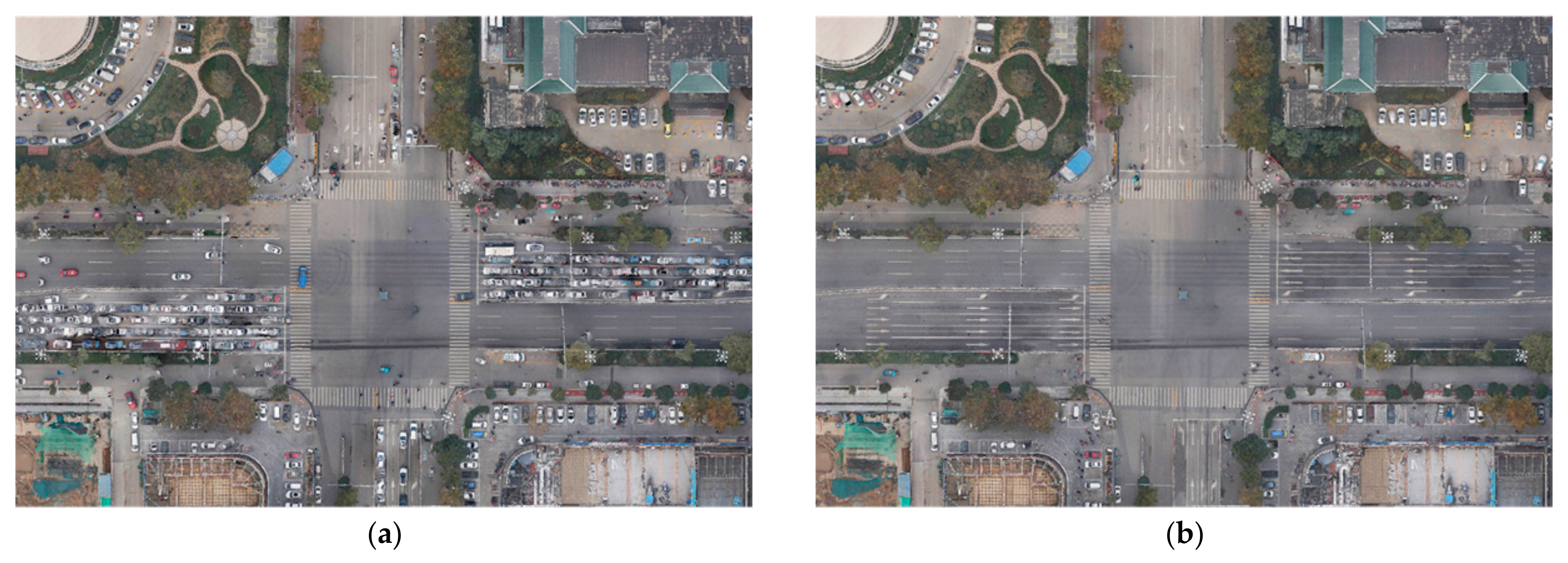
Figure 2. A comparison of the results before and after the optimization of the moving car regions (Figure (a) was obtained using the traditional reconstruction method, and Figure (b) was obtained with our method).
Remotesensing 13 03458 g002
Figure 3. Pipelines of the multiview 3D reconstruction method that integrates moving car recognition and removal.
Remotesensing 13 03458 g003
Figure 4. A schematic diagram of car information recognition based on the Mask R-CNN model.
Remotesensing 13 03458 g004
Figure 5. The recognition results of car information.
Remotesensing 13 03458 g005
Figure 6. Classification diagrams of different car states, in which Figure (a) illustrates cars in the moving state, Figure (b) and Figure (c) illustrate cars that are temporarily stationary, and Figure (d) illustrates stationary cars.
Remotesensing 13 03458 g006aRemotesensing 13 03458 g006b
Figure 7. CMS identification using multiview images.
Remotesensing 13 03458 g007
Figure 8. Loss values of model training.
Remotesensing 13 03458 g008
Figure 9. Car information detection results under different shooting conditions, in which subfigure (a) is the detection result under sunny and ortho-shooting conditions, and subfigure (b) is the detection result under cloudy and ortho-shooting conditions. Subfigure (c) shows the detection results under sunny and oblique-shooting conditions.
Remotesensing 13 03458 g009aRemotesensing 13 03458 g009b
Figure 10. The car state recognition diagram of the viaduct scene, where subfigure (a) is the original image, subfigure (b) is the geometric mesh of the scene, subfigure (c) is the different textures in the multiview images corresponding to the red frame area in subfigure (a), subfigure (d) is the detection results of car information in subfigure (a), and subfigure (e) is the recognition results of car state in Figure (d).
Remotesensing 13 03458 g010
Figure 11. The car state recognition diagram of a public parking lot, in which Figure (a) is the original image, Figure (b) is the geometric mesh of the scene, Figure (c) is the state recognition results of the cars detected in Figure (a), and Figure (d) is the results of geometric mesh clean of the car areas where the temporary stay occurred.
Remotesensing 13 03458 g011
Figure 12. The car state recognition diagram of a traffic light intersection area, in which Figure (a) is the original image, Figure (b) is the detection results of the car information in Figure (a), Figure (c) is the geometric mesh of the scene, and Figure (d) is the state recognition results of the cars detected in Figure (b).
Remotesensing 13 03458 g012
Figure 13. A comparison of the moving car removal results in urban viaduct scenes, where Figure (a) is the scene model constructed using the traditional method and Figure (b) is the 3D reconstruction result using the method in this article.
Remotesensing 13 03458 g013
Figure 14. A comparison of the removal results of moving cars in the parking lot area, where Figure (a) is the 3D model constructed using the traditional method and Figure (b) is the 3D reconstruction result after the moving cars are removed using the method in this paper.
Remotesensing 13 03458 g014
Figure 15. A comparison of the removal results of moving cars in the intersection area, where Figure (a) is the scene model constructed using the traditional method and Figure (b) is the 3D reconstruction result using the method in this article.
Remotesensing 13 03458 g015
Table 1. Experimental Environment.
NameVersion
OSUbuntu 16.04
CPUIntel Core [email protected]
GPUNVIDIA GeForce RTX 2070
LanguagePython 3.6
FrameworkTensorFlow v1.14.0 + Keras v2.1.5
Accelerator LibraryCUDA v10.0 + CUDNN v7.6
Table 2. Detection Results of Car Information.
SceneCar DetectionCar Colour
PrecisionRecallPrecision
Ortho + Sunny0.9540.9460.868
Ortho + Cloudy0.9710.9530.891
Oblique + Sunny0.9370.9250.852
Table 3. Statistic Results of Select Regions.
Regionnkn1ratio1n2ratio2State
Red Box17520.011----Moving
Blue Box168600.357----Short stay
Yellow Box1901830.9631120.612Short stay
Green Box2071950.9421730.887Stationary
Publisher’s Note: MDPI stays neutral with regard to jurisdictional claims in published maps and institutional affiliations.