Difference Curvature Multidimensional Network for Hyperspectral Image Super-Resolution

Abstract

In recent years, convolutional-neural-network-based methods have been introduced to the field of hyperspectral image super-resolution following their great success in the field of RGB image super-resolution. However, hyperspectral images appear different from RGB images in that they have high dimensionality, implying a redundancy in the high-dimensional space. Existing approaches struggle in learning the spectral correlation and spatial priors, leading to inferior performance. In this paper, we present a difference curvature multidimensional network for hyperspectral image super-resolution that exploits the spectral correlation to help improve the spatial resolution. Specifically, we introduce a multidimensional enhanced convolution (MEC) unit into the network to learn the spectral correlation through a self-attention mechanism. Meanwhile, it reduces the redundancy in the spectral dimension via a bottleneck projection to condense useful spectral features and reduce computations. To remove the unrelated information in high-dimensional space and extract the delicate texture features of a hyperspectral image, we design an additional difference curvature branch (DCB), which works as an edge indicator to fully preserve the texture information and eliminate the unwanted noise. Experiments on three publicly available datasets demonstrate that the proposed method can recover sharper images with minimal spectral distortion compared to state-of-the-art methods. PSNR/SAM is 0.3–0.5 dB/0.2–0.4 better than the second best methods.

1. Introduction

Obtained from hyperspectral sensors, a hyperspectral image (HSI) is a collection of tens to hundreds of images at different wavelengths for the same area. It contains three-dimensional hyperspectral (x, y, $\lambda$) data, where x and y represent the horizontal and vertical spatial dimensions, respectively, and $\lambda$ represents the spectral dimension. Compared to previous imaging techniques such as multi-spectral imaging, hyperspectral imaging has much narrower bands, resulting in a higher spectral resolution. Hyperspectral remote sensing imagery has a wide variety of studies from target detection, classification, and feature analysis, and has many practical applications in mineralogy, agriculture, medicine, and other fields [1,2,3,4,5,6,7]. Consequently, higher spatial-spectral resolution of hyperspectral images allows a more efficient way to explore and classify surface features.

To ensure the reception of high-quality signals with low signal-to-noise ratio, there is a trade-off between the spatial and spectral resolution of the imaging process [8,9,10]. Accordingly, HSIs are often accessed under relatively low spatial resolution, which would impede the perception of details and learning of discriminative structural features, as well as further analysis in related applications. With the hope of recovering spatial features economically, post-processing techniques such as super-resolution are an ideal way to restore details from a low-resolution hyperspectral image.

Generally, there exist two prevailing methods to enhance the spatial details, i.e., the fusion-based HSI super-resolution and single HSI super-resolution approaches. For the former category, Palsson et al. [11] proposed a 3D convolutional network for HSI super-resolution by incorporating an HSI and a multispectral image. Han et al. [12] first combined a bicubic up-sampled low-resolution HSI with a high-resolution RGB image into a CNN. Dian et al. [13] propose a CNN denoiser based method for hyperspectral and multispectral image fusion, which overcomes the difficulty of not enough training data and has achieved outstanding performance. Nevertheless, auxiliary multispectral images have fewer spectral bands than HSIs, which will cause spectral distortion of the reconstructed images. To address these drawbacks, some improvements have been made in subsequent works [14,15,16,17,18]. However, the premise is that the two images should be aligned, otherwise the performance will be significantly degraded [19,20,21]. Compared with the former, single HSI super-resolution methods require no auxiliary images, which are more convenient to apply to the real scenario. Many approaches such as sparse regularization [22] and low rank approximation [21,23] have been proposed in this direction. However, such hand-crafted priors are time-consuming and have limited generalization ability.

Currently, the convolutional neural network (CNN) has achieved great success in RGB image super-resolution tasks, and was introduced to restore the HSI. Compared with RGB image super resolution, HSI super-resolution is more challenging. On the one hand, HSIs have far more bands than RGB images and most of the bands are useful for actual analysis of surface features, but unfortunately several public datasets have much smaller training sets compared to RGB images. Hence, the network needs to preserve the spectral information and avoid distortion while increasing the spatial resolution of HSI and the design needs to be delicate enough to refrain from overfitting caused by insufficient data. To handle this problem, there have been many attempts in recent years. For instance, Li et al. [24] proposed a spatial constraint method to increase the spatial resolution as well as preserve the spectral information. Furthermore, Li et al. [25] presented a grouped deep recursive residual network (GDRRN) to find a mapping function between the low-resolution HSI and high-resolution HSI. They first combined the spectral angler mapping (SAM) loss with the mean square error (MSE) loss for network optimization, reducing the spectral distortion. Nonetheless, the spatial resolution is relatively low. To better learn spectral information, Mei et al. [26] proposed a novel three-dimensional full convolutional neural network (3D CNN), which can better learn the spectral context and alleviate distortion. In addition, [27,28] applied 3D convolution to their network. However, the use of 3D convolution requires a huge amount of computation due to the high-dimensional nature of HSI. On the other hand, there exists a large amount of unrelated redundancy in the spatial dimension, which hinders the effective processing of images. Although existing approaches try to extract texture features, it is still difficult to recover the delicate texture in the reconstructed high-resolution HSI [29,30]. For example, Jiang et al. [30] introduced a deep residual network with a channel attention module (SSPSR) and applied a skip-connection mechanism to help promote attention to high-frequency information.

To deal with the hyperspectral image super-resolution (HSI SR) problem, we propose a difference curvature multidimensional network (DCM-Net) in this paper. First, we group the input images in a band-wise manner and feed them into several parallel branches. In this way, the number of parameters can be reduced while the performance can also be improved as evidenced by the experimental results. Then, in each branch, we devise a novel multidimensional enhanced block (MEB), consisting of several cascaded multidimensional enhanced convolution (MEC) units. MEC can exploit long-range intra- and inter-channel correlations through bottleneck projection and spatial and spectral attention. In addition, we design a difference curvature branch (DCB) to facilitate learning edge information and removing unwanted noise. It consists of five convolutional layers with different filters and can easily be applied to the network to recalibrate features. Extensive evaluation of three public datasets demonstrates that the proposed DCM-Net can increase the resolution of HSI with sharper edges as well as preserving the spectral information better than state-of-the-art (SOTA) methods.

In summary, the contributions of this paper are threefold.

1.

We propose a novel difference curvature multidimensional network (DCM-Net) for hyperspectral image super-resolution, which outperforms existing methods in both quantitative and qualitative comparisons.

2.

We devise a multidimensional enhanced convolution (MEC), which leverages a bottleneck projection to reduce the high dimensionality and encourage inter-channel feature fusion, as well as an attention mechanism to exploit spatial-spectral features.

3.

We propose an auxiliary difference curvature branch (DCB) to guide the network to focus on high-frequency components and improve the SR performance on fine texture details.

The rest of the paper is organized as follows. In Section 2 we present the proposed method. The experimental results and analysis are presented in Section 3. Some ablation experiments and a discussion are presented in Section 4. Finally, we conclude the paper in Section 5.

2. Materials and Methods

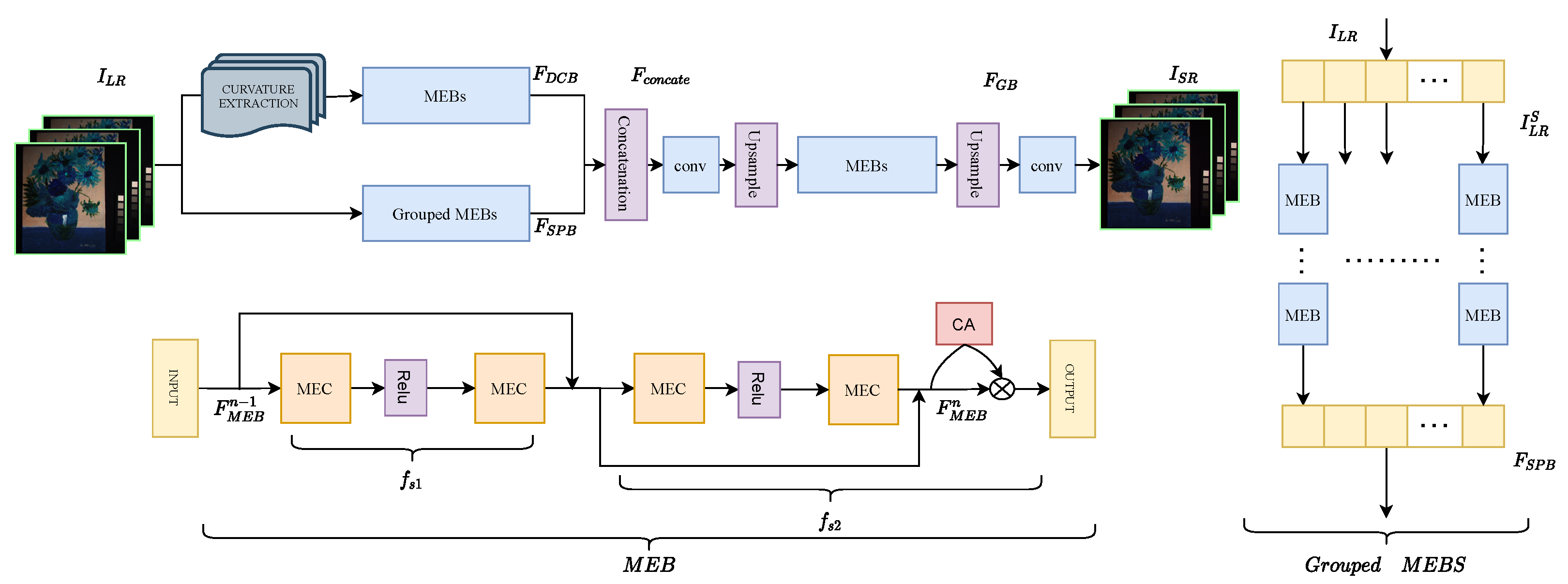
In this section, we present the proposed DCM-Net in detail, including the network structure, the multidimensional enhanced block (MEB), the difference curvature-based branch (DCB), and the loss function. The overview network structure of the proposed DCM-Net is illustrated in Figure 1.

Figure 1. The overall architecture of the proposed DCM-Net, where MEB denotes the multidimensional enhanced convolution.

2.1. Network Architecture

The network of DCM-Net mainly consists of two parts: a two-step network for deep feature extraction and a reconstruction layer. Given the input low-resolution HSI ${\mathbf{I}}_{LR}\in R^{h\times w\times c}$, we want to reconstruct the corresponding high-resolution HSI ${\mathbf{I}}_{SR}\in R^{H\times W\times C}$, where H and W (h and w) denote the height and width of the high-resolution (low-resolution) image, and C represents the number of spectral bands.

First, we feed the input ${\mathbf{I}}_{LR}\in R^{h\times w\times c}$ to two branches, a difference curvature-based branch (DCB), which is designed to further exploit the texture information, and a structural-preserving branch (SPB), which can be formulated as follows:

$${\mathbf{F}}_{\mathit{DCB}}=H_{DCB}\left({\mathbf{I}}_{\mathit{LR}}\right),$$

(1)

$${\mathbf{F}}_{\mathit{SPB}}=H_{SPB}\left({\mathbf{I}}_{\mathit{LR}}\right),$$

(2)

where ${\mathbf{F}}_{DCB}$, ${\mathbf{F}}_{SPB}$, $H_{DCB}$, $H_{SPB}$ stand for the output feature maps and the functions of DCB and SPB, respectively. The two branches both use MEB as the basic unit while in the SPB a group strategy inspired by [24] is adopted: we channel-wisely split the input image to several groups, by which we can reduce the parameters needed for the network, thus lowering the burden on the device. More importantly, given the strong correlation between adjacent spectral bands, we adopt such group strategy to promote the interaction between channels with strong spatial-spectral correlation to a certain extent.

Given that the input is ${\mathbf{I}}_{LR}$, it can be divided into multiple groups: ${\mathbf{I}}_{LR}={\mathbf{I}}_{LR}^{\left(1\right)},{\mathbf{I}}_{LR}^{\left(2\right)},\cdots ,{\mathbf{I}}_{LR}^{(\cdots )}$. Let the number of groups be S, we feed these groups ${\mathbf{I}}_{LR}^{\left(S\right)}$ into multiple MEBs to obtain the deep spatial-spectral feature, where we use a novel convolutional operation that can promote channel-wise interaction as well as exploit the long-range spatial dependency:

$${\mathbf{F}}_{\mathit{MEB}}^{\left(s\right)}=H_{\mathit{MEB}}\left({\mathbf{I}}_{\mathit{LR}}^{\left(S\right)}\right)+{\mathbf{I}}_{\mathit{LR}}^{\left(S\right)},$$

(3)

where $H_{MEB}(·)$ denotes the function of the MEBs, which we will thoroughly demonstrate in the following part.

After obtaining the outputs of both branches, we concatenate them for further global feature extraction and this can be written as $F_{concate}$. To lower the parameters needed and computational complexity, a convolutional layer is applied to reduce the dimension. It is worth noting that, considering that the pre-upsampling approach not only brings about the growth of the number of parameters but also brings about problems such as noise amplification and blurring, and post-upsampling makes it difficult to learn the mapping function directly when the scaling factor is large, we adopt a progressive upsampling method, hoping that through such a compromise, we can avoid the problems brought about by the above two upsampling methods [31,32,33]. The up-sampled values will be noted in the implementation details.

Finally, after obtaining the output of the global branch, we use a convolution layer for reconstruction:

$${\mathbf{I}}_{\mathit{SR}}=f_{rec}\left({\mathbf{F}}_{\mathit{GB}}\right),$$

(4)

where $f_{rec}(·)$ denotes the reconstruction layer and ${\mathbf{I}}_{\mathit{SR}}$ denotes the final output of the network.

2.2. Multidimensional Enhanced Block (MEB)

2.2.1. Overview

The structure of MEB is shown in Figure 2, which is designed to better learn the spectral correlation and the spatial details. Denoting ${\mathbf{F}}_{MEB}^{n-1}$ and ${\mathbf{F}}_{MEB}^n$ as the input and output of the block, and $f_{s1}$ and $f_{s2}$ as the stacked multidimensional enhanced convolution (MEC) layers, we have:

$${\mathbf{F}}_{\mathit{MEB}}^n=f_{s2}(f_{s1}\left({\mathbf{F}}_{\mathit{MEB}}^{n-1}\right)+{\mathbf{F}}_{\mathit{MEB}}^{n-1}),$$

(5)

where $f_{s1}$ and $f_{s2}$ stand for the two steps of the block. The details of MEC will be thoroughly discussed as follows.

Figure 2. The architecture of MEC.

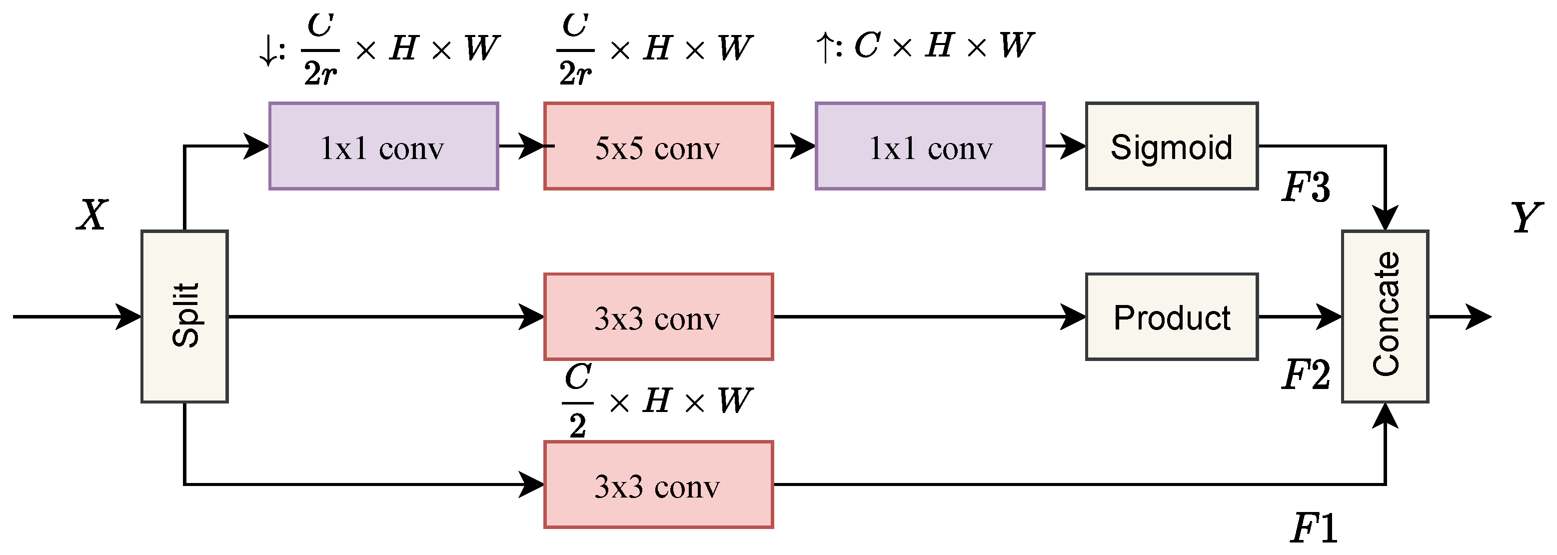
2.2.2. Multidimensional Enhanced Convolution (MEC)

The residual network structure proposed by He et al. [34] has been widely used in many image restoration tasks and achieved impressive performance. However, as mentioned before, dealing with HSI is more tricky, since standard 2D convolution is inadequate to explicitly extract discriminating feature maps from the spectral dimensions, while 3D convolution is more computationally costly. To address this issue, we introduce an effective convolution block to better exploit spectral correlation and reduce the redundancy in the spectral dimension while preserving more useful information.

Specifically, given the input X, we first channel-wisely split it into two groups to reduce the computational burden. Furthermore, we add a branched path in one of the groups; in this path, $1\times 1$ convolution is applied as cross-channel pooling [35] to reduce the spectral dimensionality instead of spatial dimensionality, which indeed performs a linear recombination on the input feature maps and allows information interaction between channels. Besides, the structure builds long-range spatial-spectral dependencies, which can further improve the network’s performance. In addition, the parameters can also be reduced, which allows us to apply $5\times 5$ convolution and enlarge the fields of view. Given the input $\mathbf{X}$, the formulation is presented as follows:

$${\mathbf{F}}_1={\mathbf{F}}_2=f_{3\times 3}\left({\mathbf{X}}^{\frac{\mathbf{C}}{\mathbf{2}}\times \mathbf{H}\times \mathbf{W}}\right),$$

(6)

$${\mathbf{F}}_3=\sigma \left(f_{1\times 1}\left(f_{5\times 5}\left(f_{1\times 1}\left({\mathbf{X}}^{\frac{\mathbf{C}}{\mathbf{2}\mathbf{r}}\times \mathbf{H}\times \mathbf{W}}\right)\right)\right)\right),$$

(7)

$$\mathbf{Y}=f_{concate}(({\mathbf{F}}_2\times {\mathbf{F}}_3),{\mathbf{F}}_1),$$

(8)

where $f_{1\times 1}$ and $f_{3\times 3}$ denote $1\times 1$ convolution and $3\times 3$ convolution, respectively. ${\mathbf{F}}_1$ and ${\mathbf{F}}_2$ are the outputs of the upper and lower branches in Figure 2. $\sigma$ is the sigmoid function; the setting of r will be mentioned in the implementation details.

2.2.3. Attention-Based Guidance

The attention mechanism is a prevalent practice in CNNs nowadays. It allows the network to attend to specific regions in the feature maps to emphasize important features. To further improve the ability of spectral correlation learning, we apply the channel attention module proposed by Zhang et al. [36] in the final part of the MEB. Specifically, with the input ${\mathbf{F}}_{\mathit{MEB}}^n$, a spatial global pooling operation is used to aggregate the spatial information:

$$\mathbf{z}=H_{\mathit{GP}}\left({\mathbf{F}}_{\mathit{MEB}}^n\right),$$

(9)

where $H_{\mathit{GP}}$ denotes the spatial global pooling. Then, a simple gating mechanism with a sigmoid function is applied:

$$\mathbf{s}=f_{CA}\left(\mathbf{z}\right),$$

(10)

where $f_{CA}$ denotes the gating mechanism. $\mathbf{s}$ is the attention map, which is used to re-scale the input ${\mathbf{F}}_{\mathit{MEB}}^n$ via an element-wise multiplication operation:

$${\mathbf{F}}_{\mathit{MEB}}^n=\mathbf{s}\times {\mathbf{F}}_{\mathit{MEB}}^n.$$

(11)

2.3. Difference Curvature-Based Branch (DCB)

In the field of computer vision, there is a long history of using the gradient or curvature to extract texture features. For example, Chang et al. [37] simply concatenated the first-order and second-order gradients for feature representation based on the luminance values of the pixels in the patch. Zhu et al. [38] proposed a gradient-based super-resolution method to exploit more expressive information from the external gradient patterns. In addition, Ma et al. [39] applied a first-order gradient to a generative adversarial network (GAN)-based method as structure guidance for super-resolution. Although they can extract high-frequency components, simple concatenation of gradients also brings undesired noise, which hinders feature learning. Compared with the gradient-based method, curvature is better for representing high-frequency features. There exist three main kinds of curvature: Gaussian curvature, mean curvature, and difference curvature. Chen et al. [40] proposed and applied difference curvature as an edge indicator for image denoising, which is able to distinguish isolated noise from the flat and ramp edge regions and outperforms Gaussian curvature and mean curvature. Later, Huang et al. [41] applied difference curvature for selective patch processing and learned the mixture prior models in each group. As for the hyperspectral image, due to its high dimensionality and relatively low spatial resolution, it is necessary to extract fine texture information efficiently to increase the spatial resolution.

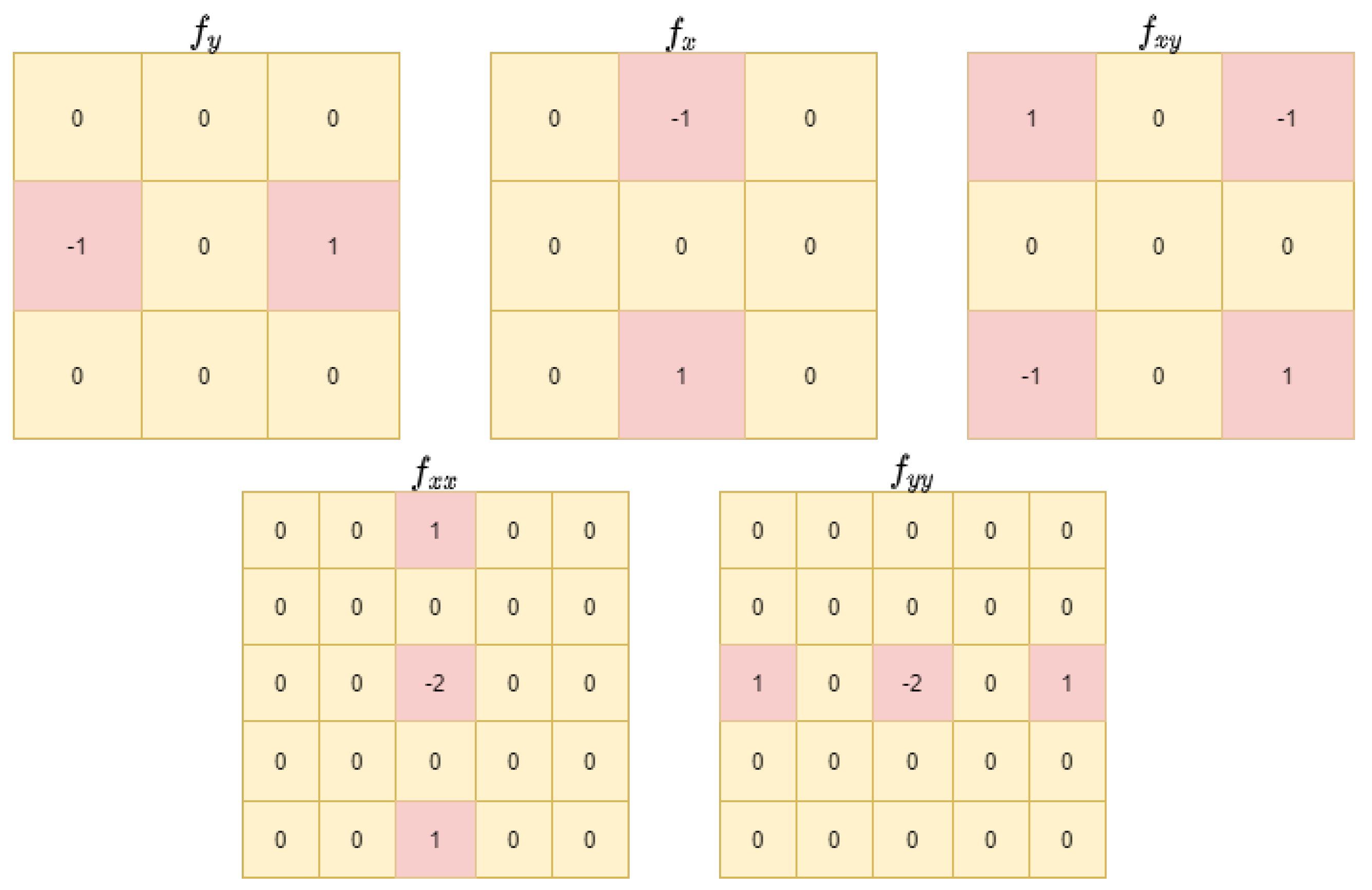
To efficiently exploit the texture information of HSI, we designed an additional DCB to help the network focus on high-frequency components. Compared with traditional gradient-based guidance, which cannot effectively distinguish between edges and ramps, difference curvature combines the first- and second-order gradients, which are more informative. Consequently, it can effectively distinguish edges and ramps together whiling removing unwanted noise. The difference curvature can be defined as follows:

$$\mathbf{D}=\left|\left|{\mathbf{f}}^{ϵ}\right|-\left|{\mathbf{f}}^{\mu }\right|\right|,$$

(12)

where ${\mathbf{f}}_i^{ϵ}$ and ${\mathbf{f}}_i^{\mu }$ are defined as:

$${\mathbf{f}}^{ϵ}=\frac{{\mathbf{f}}_x^2{\mathbf{f}}_{xx}+2{\mathbf{f}}_x{\mathbf{f}}_y+{\mathbf{f}}_y^2{\mathbf{f}}_{yy}}{{\mathbf{f}}_x^2+{\mathbf{f}}_y^2},$$

(13)

$${\mathbf{f}}^{\mu }=\frac{{\mathbf{f}}_x^2{\mathbf{f}}_{xx}-2{\mathbf{f}}_x{\mathbf{f}}_y+{\mathbf{f}}_y^2{\mathbf{f}}_{yy}}{{\mathbf{f}}_x^2+{\mathbf{f}}_y^2}.$$

(14)

As demonstrated in Figure 3, the curvature calculation is easy to implement by using five convolution kernels $({\mathbf{f}}_x,{\mathbf{f}}_y,{\mathbf{f}}_{xx},{\mathbf{f}}_{yy},{\mathbf{f}}_{xy})$ to extract the first- and second-order gradients. The five kernels are ${\mathbf{f}}_x=\left[0,-1,0;0;0,1,0\right]$, ${\mathbf{f}}_y=\left[0;-1,0,1;0\right]$,

Figure 3. The convolution kernels for curvature extraction.

${\mathbf{f}}_{xx}=\left[0,0,1,0,0;0;0,0,-2,0,0;0;0,0,1,0,0\right]$, ${\mathbf{f}}_{yy}=\left[0;0;1,0,-2,0,1;0;0\right]$, and ${\mathbf{f}}_{xy}=\left[1,0,-1;0;-1,0,1\right]$.

Based on these, the calculated difference-curvature has the following properties in different image regions. (1) $\left|{\mathbf{f}}^{ϵ}\right|$ is large but $\left|{\mathbf{f}}^{\mu }\right|$ is small for edges, so $\mathbf{D}$ is large; (2) for smooth regions, $\left|{\mathbf{f}}^{ϵ}\right|$ and $\left|{\mathbf{f}}^{\mu }\right|$ are both small, so $\mathbf{D}$ is small; and (3) for noise, $\left|{\mathbf{f}}^{ϵ}\right|$ is large but $\left|{\mathbf{f}}^{\mu }\right|$ is also large, so $\mathbf{D}$ is small. Therefore, most parts of the curvature map have small values, and only high frequency information is preserved. After the extraction module, we feed the curvature map into multiple MEBs to obtain higher-level information. Then, as shown in Figure 1, the output of the branch is fused with the features from the main branch. In this way, DCB guides the network to focus on high-frequency components and improve the SR performance on fine texture details.

2.4. Loss Function

In previous image restoration works in recent years, L1 loss and MSE loss have been two widely used losses for network optimization. In the field of HSI super-resolution, previous works have also explored other losses, such as SAM loss [24] and SSTV loss [30], considering the special characteristics of HSI. These losses encourage the network to preserve the spectral information. Following the practice, we add the SSTV loss to the L1 loss [30] as the final training objective of our DCM-Net, i.e.,

$${\mathcal{L}}_{SSTV}=\frac{1}{N}\sum _{n=1}^N({∥{\nabla }_h{\mathbf{I}}_{SR}^n∥}_1+{∥{\nabla }_w{\mathbf{I}}_{SR}^n∥}_1+{∥{\nabla }_c{\mathbf{I}}_{SR}^n∥}_1),$$

(15)

$${\mathcal{L}}_1=\frac{1}{N}\sum _{n=1}^N\left({∥{\mathbf{I}}_{HR}^n-H_{DCM-Net}\left({\mathbf{I}}_{LR}^n\right)∥}_1\right),$$

(16)

$${\mathcal{L}}_{total}\left(\theta \right)={\mathcal{L}}_1+\alpha {\mathcal{L}}_{SSTV},$$

(17)

where ${\mathbf{I}}_{LR}^n$ and ${\mathbf{I}}_{HR}^n$ represent the n-th low-resolution image and its corresponding high-resolution one. $H_{DCM-Net}$ denotes the proposed network. ${\nabla }_h$, ${\nabla }_w$, and ${\nabla }_w$ denote the horizontal, vertical, and spectral gradient calculation operators, respectively. The setting of the hyper-parameter $\alpha$ that balances the two losses follows the previous work [30], i.e., it is set to $0.001$ in this paper.

2.5. Evaluation Metrics

We adopted six prevailing metrics to evaluate the performance from both the spatial and spectral aspects. These metrics include the peak signal-to-noise ratio (PSNR), structure similarity (SSIM) [42], spectral angle mapper (SAM) [43], cross correlation (CC) [44], root mean square error (RMSE), and erreur relative globale adimensionnelle de synthese (ERGAS) [45]. PSNR and SSIM are widely used to assess the similarities between images, while the remaining four metrics are often used to evaluate the HSI: CC is a spatial measurement, SAM is a spectral measurement, RMSE and ERGAS are global measurements. In the following experiments, we regard PSNR, SSIM, and SAM as the main metrics, which are defined as follows:

$$PSNR=\frac{1}{L}\sum _{l=1}^L(10{log}_{10}(\frac{{MAX}_l^2}{MS{E}_l})),$$

(18)

$${MSE}_l=\frac{1}{WH}\sum _{w=1}^W\sum _{h=1}^H({\mathbf{I}}_{SR}(w,h,l)-{\mathbf{I}}_{HR}(w,h,l)),$$

(19)

$$SSIM=\frac{1}{L}\sum _{l=1}^L\frac{(2{\mu }_{{\mathbf{I}}_{SR}}^l{\mu }_{{\mathbf{I}}_{HR}}^l+c_1)(2{\sigma }_{{\mathbf{I}}_{SR}{\mathbf{I}}_{HR}}^l+c_2)}{a\times b},$$

(20)

$$a={({\mu }_{{\mathbf{I}}_{SR}}^l)}^2+{({\mu }_{{\mathbf{I}}_{HR}}^l)}^2+c_1,$$

(21)

$$b={({\sigma }_{{\mathbf{I}}_{SR}}^l)}^2+{({\sigma }_{{\mathbf{I}}_{HR}}^l)}^2+c_2,$$

(22)

$$SAM(x_i,\widehat{x_i})=arccos(\frac{⟨{\mathbf{I}}_{SR}{\mathbf{I}}_{HR}⟩}{{∥{\mathbf{I}}_{SR}∥}_2{∥{\mathbf{I}}_{HR}∥}_2}),$$

(23)

where ${MAX}_l$ denotes the maximum pixel value in the l-th band, and ${\mu }_{{\mathbf{I}}_{SR}}$, ${\mu }_{{\mathbf{I}}_{HR}}$ represent the mean of ${\mathbf{I}}_{SR}$ and ${\mathbf{I}}_{HR}$, respectively. ${\sigma }_{{\mathbf{I}}_{SR}}^l$ and ${\sigma }_{{\mathbf{I}}_{HR}}^l$ denote the variance of ${\mathbf{I}}_{SR}$ and ${\mathbf{I}}_{HR}$ in the l-th band while ${\sigma }_{{\mathbf{I}}_{SR}{\mathbf{I}}_{HR}}$ is the covariance of ${\mathbf{I}}_{SR}$ and ${\mathbf{I}}_{HR}$ in the l-th band. $⟨·⟩$ denotes the dot product operation.

2.6. Datasets

1.

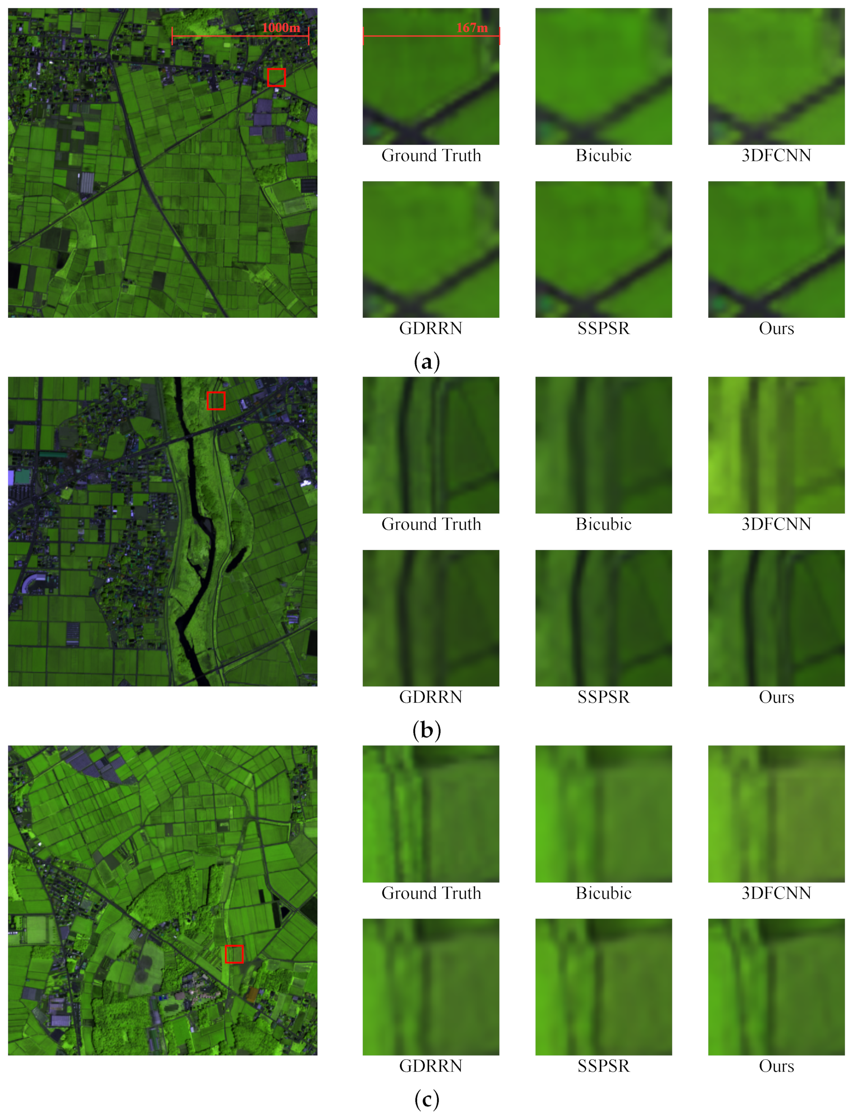
Chikusei dataset [46]: the Chikusei dataset (https://www.sal.t.u-tokyo.ac.jp/hyperdata/ accessed on 29 July 2014) was taken by the Headwall Hyperspec-VNIR-C imaging sensor over agricultural and urban areas in Chikusei, Ibaraki, Japan. The central point of the scene is located at coordinates 36.294946N, 140.008380E. The hyperspectral dataset has 128 bands in the spectral range from 363 nm to 1018 nm. The scene consists of 2517 × 2335 pixels and the ground sampling distance was 2.5 m. A ground truth of 19 classes was collected via a field survey and visual inspection using high-resolution color images obtained by a Canon EOS 5D Mark II together with the hyperspectral data.

2.

Cave dataset [47]: the Cave dataset (https://www.cs.columbia.edu/CAVE/databases/multispectral/ accessed on 29 April 2020) was obtained from Cooled CCD camera and contains full spectral resolution reflectance data from 400 nm to 700 nm at a resolution of 10 nm (31 bands in total), covering 32 scenes of everyday objects. The image size is 512 × 512 pixels and each image is stored as a 16-bit grayscale PNG image per band.

3.

Harvard dataset [48]: the Harvard Dataset (http://vision.seas.harvard.edu/hyperspec/index.html accessed on 29 April 2020) contains fifty images captured under daylight illumination from a commercial hyperspectral camera (Nuance FX, CRI Inc. in U.S.), which is capable of acquiring images from 420 nm to 720 nm at a step of 10 nm (31 bands in total).

2.7. Implementation Details

Because the numbers of spectral bands in the three datasets are different, the experiment setting varies. For the Chikusei dataset, we divided 128 bands into 16 groups, i.e., 8 bands per group. For the Cave and Harvard datasets, which both have 31 bands, we put 4 bands in one group with an overlap of one band between each group (10 groups). The number of MEBs was set to 3 for Chikusei and 6 for Cave and Harvard. As for the MEC module, we applied two $1\times 1$ convolutions to reduce the dimension by half. For the $3\times 3$ convolution, to keep the spatial size of feature maps, the padding size was set to 1. We implemented the network with PyTorch and optimized it using the ADAM optimizer with an initial learning rate of $1\times {10}^{-4}$, which was halved by every 15 epochs. The batch size was 16.

3. Results

In this section, we describe the experiments conducted to evaluate the effectiveness of the proposed DCM-Net and compare it with existing single HSI super-resolution methods on three public datasets, which will be discussed in detail in the following sections.

3.1. Results for the Chikusei Dataset

Taken by the Headwall Hyperspec-VNIR-C imaging sensor over agricultural and urban areas in Chikusei, Ibaraki, Japan, the hyperspectral dataset has 128 bands in the spectral range from 363 nm to 1018 nm [46]. To be consistent with previous works [30], we followed the the same setup and crop four images with 512 × 512 × 128 pixels for testing and used the rest for training (3226 pics for scale factor of 2, and 3119 pics for $\times 4$, 757 for $\times 8$). The results for the different methods are summarized in Table 1. As can be seen, at a scale factor of 2, we have the greatest advantage, with psnr 0.58 dB higher than the second best result and SAM 0.09 lower than the second best result; when the scale factor is 4, the (PSNR/SAM/SSIM) is (0.18 dB, 0.05, 0.005) better than SSPSR; at a scale factor of 8, we also achieved the best performance.

Table 1. Quantitative comparison of different methods for the Chikusei dataset.

	Scale Factor	MPSNR↑	SAM↓	ERGAS↓	MSSIM↑	RMSE↓	CC↑
Bicubic		43.2125	1.7880	3.5981	0.9721	0.0082	0.9781
3DCNN		43.3474	2.0869	3.9442	0.9738	0.0082	0.9756
GDRRN	2	44.3162	1.9147	3.6428	0.9807	0.0068	0.9803
SSPSR		47.4403	1.2072	2.2805	0.9897	0.0050	0.9910
DCM-NET		48.0238	1.1160	2.1766	0.9906	0.0047	0.9916
Bicubic		37.6377	3.4040	6.7564	0.8954	0.01560	0.9212
3DCNN		37.7371	3.6217	6.9364	0.9013	0.0153	0.9197
GDRRN	4	38.0868	3.4031	6.8083	0.9151	0.0142	0.9259
SSPSR		40.3612	2.3527	4.9894	0.9413	0.0114	0.9565
DCM-NET		40.5139	2.3012	4.8584	0.9464	0.0112	0.9581
Bicubic		34.5049	5.0436	9.6975	0.8069	0.0224	0.8314
3DCNN		34.8409	4.9703	9.6065	0.8241	0.0209	0.8463
GDRRN	8	35.2210	4.6363	9.0720	0.8354	0.0202	0.7977
SSPSR		35.8279	4.0282	8.3177	0.8538	0.0192	0.8773
DCM-NET		35.9809	3.9310	8.1459	0.8580	0.0189	0.8811

To further illustrate the superiority of DCM-Net, we present the visual results in Figure 4 as well as their spectral curves in Figure 5. As can be seen, it is obvious that our method outperforms others. In Figure 4a, there is a thin light-colored line along the dark black thick line in the ground truth image, which is not captured and restored by 3DFCNN. Although it can be observed in the results reconstructed by GDRRN and SSPSR, the line is too inconspicuous to be easily detected. By contrast, our method can preserve the details, making it much clearer. In Figure 4b, compared with the results by other methods, which are blurry, our DCM-Net yields a better result with clear details, e.g., the edge is sharper and the structure is more consistent. In Figure 4c, there are two very close lines in the ground truth image, which are hardly distinguished in the results by other methods. By contrast, these two lines can still be observed in our result, demonstrating that our DCM-Net can exploit the spectral interactions and benefit from the difference-curvature guidance to reconstruct fine edges. Subsequently, we also present the spectral curves of the three test images and their super-resolution results in Figure 5, which is yielded by ENVI (remote-sensing software that provides hyperspectural image analysis, image enhancement, and feature extraction). We can see that the curves of 3DFCNN, GDRRN, and SSPSR are very close to the bicubic interpolation, implying a limited performance for the restoration of spectral information. By contrast, the curve of our DCM-Net is close to the ground truth, demonstrating that our network can better preserve spectral information and avoid distortions. In addition, we show the absolute error maps of these three images in Figure 6. Usually, the bluer the image is, the closer the reconstructed image is to the original image; here again, it can be seen that our reconstructed method is better able to preserve edge features.

Figure 4. Visual results of the three reconstructed images (a–c) of the Chikusei dataset for different SR methods. Scale factor is 2. Bands 70/100/36 are treated as the R/G/B channels for visualization. As can be seen in all three figures, for the recovery of lines, especially those in close proximity to each other, we were able to recover better.

Figure 5. The spectral curves corresponding to the three reconstructed images (a–c) in Figure 4 by different methods.

Figure 6. The absolute error maps corresponding to the three reconstructed images (a–c) in Figure 4 by different methods.

3.2. Results for the Cave Dataset

Different from the Chikusei Dataset, which was obtained from a remote sensing camera, the Cave dataset obtained from a cooled CCD camera contains full spectral resolution reflectance data from 400 to 700 nm at a resolution of 10 nm (31 bands in total), covering 32 scenes of everyday objects [47]. The images are of size 512 × 512 pixels and are stored as 16-bit grayscale PNG images per band. We randomly chose 8 scenes for testing and used the left images during training. They were randomly cropped into the size of 32 × 32 pixels, 64 × 64 pixels, and 128 × pixels, when the scale factors were 2, 4, and 8, respectively (1555 pics for scale factors of 2, 4, and 8).

The same as for the Chikusei dataset, we tested our method on the Cave dataset at three scale factors and compared it with three recent approaches, i.e., 3DFCNN, GDRRN, and SSPSR. The results are reported in Table 2. As can be seen, our DCM-Net outperforms the second best method to varying degrees. To better illustrate that, we also show the visual results of two test images in the Cave dataset by different methods in Figure 7, absolute maps in Figure 8, and their spectral curves in Figure 9. By comparing the absolute error maps of different methods it is not difficult to find that the absolute error map generated by our method is bluer, especially around the edges. This indicates that our ability to recover texture information is better and the recovered image is closest to the original image. In general, the above results show that our network not only gains better performance on HSI images with hundreds of bands, but also outperforms other methods on the multispectral dataset.

Table 2. Quantitative comparison of different methods for the Cave dataset.

	Scale Factor	MPSNR↑	SAM↓	ERGAS↓	MSSIM↑	RMSE↓	CC↑
Bicubic		38.0603	3.2370	4.9579	0.9662	0.0147	0.9907
3DCNN		38.8706	4.0307	4.3886	0.9663	0.0131	0.9924
GDRRN	2	39.2550	3.7454	4.2106	0.9683	0.0126	0.9929
SSPSR		41.3895	3.1472	3.3333	0.9752	0.0101	0.9953
DCM-NET		41.9867	2.7051	3.1217	0.9771	0.0095	0.9957
Bicubic		33.0421	4.7962	7.8460	0.9202	0.0258	0.9767
3DCNN		33.8198	5.6688	7.6617	0.9224	0.0236	0.9780
GDRRN	4	34.4236	5.0185	6.7641	0.9361	0.0219	0.9825
SSPSR		35.3433	4.1654	6.5045	0.9434	0.0200	0.9838
DCM-NET		35.5055	3.9460	6.4092	0.9445	0.0197	0.9843
Bicubic		29.2466	6.6079	12.2687	0.8320	0.0390	0.9439
3DCNN		30.0771	7.6626	11.5550	0.8463	0.0359	0.9518
GDRRN	8	30.3026	7.1510	11.0352	0.8513	0.0353	0.9533
SSPSR		31.1290	5.5101	10.1804	0.8749	0.0325	0.9595
DCM-NET		31.3766	5.3067	9.9363	0.8822	0.0316	0.9618

Figure 7. Visual results of two reconstructed images (a,b) of the Cave dataset for different SR methods. Scale factor is 2. Bands 10/30/21 are treated as the R/G/B channels for visualization.

Figure 8. Absolute error maps corresponding to the two reconstructed images (a,b) in Figure 7 by different methods.

Figure 9. The spectral curves corresponding to the two reconstructed images (a,b) in Figure 7 by different methods.

3.3. Results for the Harvard Dataset

The Harvard dataset contains fifty images captured under daylight illumination from a commercial hyperspectral camera (Nuance FX, CRI Inc., Woburn, MA, USA), which is capable of acquiring images from 420 to 720 nm at a step of 10 nm (31 bands in total) [48]. For training, we randomly selected 90% of the images (45 images) and cropped them into $32\times 32$ patches, $64\times 64$ patches, and $128\times 128$ patches when the scale factors were 2, 4, and 8, respectively. We used the other 5 images for testing (3888 pics for scale factors of 2, 4, and 8).

Table 3 summarizes the results of different approaches on the Harvard dataset for scale factors 2, 4, and 8. As can be seen, the results here are different from our performance on Chikusei and Cave; our method is slightly behind the SSPSR when the scale factor is 2, while we have a clear advantage when the scale factor is 8. To better illustrate the superiority of our DCM-Net, we present the super-resolution results of a test image from the Harvard dataset by different methods in Figure 10. Here we chose the scale factor 8 to illustrate the robustness of our method. From Figure 10b, we can see that the super-resolution images by 3DFCNN and GDRRN are very blurry. Besides, white grid artifacts can be found in their zoom-in results. As for SSPSR, it recovers sharper images at the first glance. However, many structures in the original images have been lost. For such a large scale factor, although our DCM-Net does not recover the fine structures of the words, it indeed captures the outline of the words without causing geometry-inconsistency, which is closest to the ground truth. As for Figure 10a, it is also obvious that among all the methods, DCM-Net yields a super-resolution image with few structural distortions.

Table 3. Quantitative comparison of different methods for the Harvard dataset.

	Scale Factor	MPSNR↑	SAM↓	ERGAS↓	MSSIM↑	RMSE↓	CC↑
Bicubic		48.4963	2.7820	2.8659	0.9785	0.0056	0.9721
3DCNN		49.1729	2.8882	2.6007	0.9846	0.0047	0.9775
GDRRN	2	49.2539	2.8540	2.5774	0.9848	0.0046	0.9779
SSPSR		50.2929	2.7017	2.2116	0.9871	0.0041	0.9841
DCM-NET		50.2559	2.7389	2.2166	0.9856	0.0042	0.9829
Bicubic		43.7975	3.2996	4.6179	0.9471	0.0101	0.9352
3DCNN		44.0104	3.6372	4.5179	0.9504	0.0091	0.9415
GDRRN	4	44.0918	3.5741	4.4469	0.9504	0.0091	0.9432
SSPSR		45.2164	3.4292	3.9324	0.9552	0.0082	0.9510
DCM-NET		45.4087	3.3102	3.7988	0.9557	0.0080	0.9543
Bicubic		39.5065	3.7196	6.9913	0.9083	0.0165	0.8868
3DCNN		40.3186	4.3056	6.5590	0.9131	0.0148	0.8960
GDRRN	8	40.4038	4.1746	6.4915	0.9137	0.0147	0.8989
SSPSR		40.7316	3.6438	5.9926	0.9213	0.0138	0.9169
DCM-NET		41.2203	3.6520	5.8124	0.9220	0.0135	0.9176

Figure 10. Visual results of two reconstruted images (a,b) of the Harvard Dataset for different SR methods. Scale factor is 8. Bands 10/30/21 are treated as the R/G/B channels for visualization.

4. Discussion

4.1. Analysis on Loss Function

The choice of the loss function is crucial for reconstructing high-quality images, and here we mainly experiment and discuss for L1.MSE and the SSTV loss we use. In previous work, people preferred to use MSE loss to train their networks, because it is believed that MSE loss converges faster and yields better metrics [24,25,49]. However, through the experiments we conducted, it can be seen in Table 4 that MSE loss is not a good choice for HSI SR. First, as can be seen from the loss graph in Figure 11, when it is close to optimum, its derivatives are too small and the learning slows down, and this actually makes the network convergence time much longer than expected. In addition, studies have shown that MSE loss yields images of relatively poor perceptual quality because there is a strong penalty for large errors and a low penalty for small errors, and if a texture or mesh appears, then optimizing MSE may smooth out this area [50]. Spatial-spectral total variation (SSTV) was proposed by Aggarwal et al. [51] and was applied as a loss function by Jiang et al. [30], and it is presumed to encourage the network to reserve spatial-spectral information and avoid distortion. Through the experiment, we can confirm that although there is a certain improvement in SSTV loss compared with L1 loss, the improvement is very limited because the main body of this loss is still L1 loss.

Table 4. Ablation study of the loss function for the Chikusei dataset. Scale factor is 4.

	PSNR	SAM	SSIM
SSTV loss	40.5139	2.3012	0.9464
L1	40.4977	2.3213	0.9453
MSE	40.1801	2.4821	0.9422

Figure 11. The curves yielded by different loss functions. It is worth stating that because the training loss curves of L1 and SSTV are too close, only one line can be visually observed on the tensorboard, and the curve of SSTV is covered by the blue line.

4.2. Analysis of Multidimensional Enhanced Convolution (MEC)

Before we discuss the impact that MEC brings to our network, we experimented on MEC with two popular structures, res2net [52] and SCConv [53], which inspired our design and modification of MEC in the initial phase of the experiment (presented in Figure 12). In 2019, Gao et al. [52] constructed a new CNN structure, Res2Net, which represents multi-scale features at the granularity level and enlarges the perceptual field of each layer by constructing hierarchical residual connections within a single residual block, and claimed that it can be used in state-of-the-art backbone networks. Then in 2020, Liu et al. [53] proposed a novel self-calibrated convolution, SCConv, which models long-range dependencies as well as enlarging fields of view by average-pooling. It can also be plugged into any network to augment standard convolution. However, according to the Table 5, neither structure performs well in this experiment, and this is mainly due to the small amount of data provided by the hyperspectral image dataset. In the res2net experiment, the loss of the training set keeps decreasing, while the validation loss keeps failing to converge. SCConv reduces overfitting and accelerates convergence to some extent by adding pooling but it does not get a good result, which may be attributed to pooling again, and which deprives the network of some information that is essential for image reconstruction [54].

Figure 12. The structure of res2net and SCConv.

Table 5. Exploring different structures of MEC on the Chikusei dataset. Scale factor is 4.

	PSNR	SAM	SSIM	MACs(G)	Params(M)
MEC	40.5139	2.3012	0.9464	41.89	10.96
SCConv	38.23495	3.731482	0.913639	110.47	48.46
res2net	33.32135	7.953455	0.749981	50.95	17.63

Next, we performed an ablation study of MEC. In Table 6, “Our” and “Our-w/o MEC” denote the model equipped both modules and the model without MEC, which only uses standard convolutions instead. As can be seen, after removing MEC, PSNR drops 0.16 dB and SAM is 0.06 higher. The results clearly demonstrate that MEC outperforms standard convolutions and can better learn the spatial and spectral correlation. It not only improves the spatial resolution but also avoids the spectral distortion.

Table 6. Ablation study of the proposed-Net on the Chikusei dataset. Scale factor is 4.

	PSNR	SAM	SSIM	MACs(G)	Params(M)
Our	40.5139	2.3012	0.9464	41.89	10.96
Our-w/o DCB	40.4432	2.3419	0.9453	38.93	10.22
Our-w/o MEC	40.3846	2.3639	0.9447	58.98	20.3
Our-w/o CA	40.4432	2.3236	0.9458	41.28	10.76

More importantly, using MEC reduces the parameters by a factor of two and saves nearly 10(G) of computation compared to using normal $3\times 3$ convolution.

4.3. Difference Curvature-Based Branch (DCB)

The additional difference-curvature branch is designed to extract the curvature and provide guidance information for the network to preserve the texture and fine details. As can be seen from Table 6, without DCB, the PSNR of “Our-w/o DCB” is 0.10 dB lower than that of “Our”, demonstrating the effectiveness of the DCB. Besides, the SSIM and SAM scores are also inferior to those of “Our”. In addition, we show the visual results after curvature extraction in Figure 13 and from which it is clear that after curvature extraction, the edges are well preserved and we wish to use it to guide the network to focus on the texture and edge areas to preserve the fine details in the super-resolution results. On the right side of Figure 13, the visual differences between our method with and without DCB are presented and it can be seen that with the help of DCB, the lines of the image are sharper and more detailed features are preserved. Most importantly, the module does not bring too much computational burden.

Figure 13. Visual results after curvature extraction.

It is worth noting that, although DCB tends to recover sharper images, this does not usually mean a significant increase in the numerical index, but certainly improves the visual quality.

4.4. Analysis of Channel Group Numbers

The application of grouping strategy in hyperspectral images actually exists in many different forms [25,30,55], and they all aim at reducing the computational overhead and making the subsequent upscaling operation feasible, especially for hyperspectral images with a much smaller data volume than RGB images but several hundred channels; the grouping strategy is theoretically important to ensure the network performance while avoiding the network being too wide and too difficult to train. To better understand the impact of the grouping approach on both computational overhead and network performance, we conducted some experiments on the number of groups. First of all, the experimental combinations we chose were 1, 16, 20, and 25. Next, we selected PSNR, SAM and SSIM as indicators of image reconstruction quality. Multiply and accumulation per second (MACs(G)) and Params(M) indicate the calculating overhead and parameters needed. As we can see from Table 7, firstly, without group strategy, although the computational overhead of the network remains consistent with that of a grouped network, its required parameters are greatly increased. This makes it much more difficult for the network to process hyperspectral data with a generally small number of training sets. Therefore, a dimensionality reduction strategy like grouping is effective. After experimenting with multiple groupings, we set the number of groupings to 20, taking into account the computational overhead and the performance of the network.

Table 7. Ablation study of group number.

Group Number	PSNR	SAM	SSIM	MACs(G)	Params(M)
1	40.2285	2.3795	0.9428	45.70	60.99
16	40.3846	2.3639	0.9447	38.44	10.95
20	40.5139	2.3012	0.9464	41.89	10.96
25	40.5159	2.2892	0.9464	53.76	10.95

4.5. Analysis on Attention-Driven Guidance

Channel attention has been verified as a very effective tool for learning the channel correlation and has been adopted by various methods in different fields [30,36,56]. We tested this mechanism on the Chikusei dataset with a scaling factor of 4. What can be seen from Table 6 is that, without channel attention, our network performs the worst on SAM, which means the worst capability of learning spectral correlation. In addition, both PSNR and SSIM have declined to varying degrees. In the case of comparing the computation with and without CA, adding CA actually does not bring too much computational overhead, which also shows that it does not improve the effect by blindly increasing the computation. For hyperspectral images with hundreds of spectral bands, CA undoubtedly plays an important role.

4.6. Complexity Analysis

As can be seen on Table 8, although the network consisting of two branches looks very complex, we reduced the computational overhead of the model by applying some methods. First of all, by applying parameter sharing, the number of parameters has been reduced by at least 70 percent. The grouping strategy we used reduced the required parameters and computational overhead while ensuring the performance of the network; without the grouping function, the network needs to be wider and deeper to keep up the performance. In addition, by using MEC instead of standard $3\times 3$ convolution, we lowered the param(M) from 20.3 to 10.96, and MACs(G) from 58.98G to 41.89G.

Table 8. Efficient study of different methods.

	MACs(G)	Params(M)
3DFCNN	0.3	0.039
GDRRN	0.76	0.589
SSPSR	43.63	13.56
DCM-NET	41.89	10.96

5. Conclusions

In this paper, we proposed a deep difference curvature-based network with multidimensional enhanced convolutions for HSI super-resolution. Specifically, to reduce the redundancy as well as better exploit the spectral information, we introduced a multidimensional enhanced convolution unit into the network, which can learn the useful spectral correlation through a self-attention mechanism and a bottleneck projection. In addition, we designed an additional difference curvature branch to extract the delicate texture features of a hyperspectral image. This works as an edge indicator to fully preserve the texture information and eliminates the unwanted noise. Experiments on three public datasets demonstrated that our method is able to recover finer details and yield sharper images with minimal spectral distortion compared to state-of-the-art methods. Despite the good results obtained by the network, it is still difficult to apply in real-world applications due to the heavy computational overhead. We understand the difficulty and significance of hardware-based implementation of high-quality super-resolution, and we will next work on making the network lightweight and able to be applied on hardware.