Article

Determining Temporal Uncertainty of a Global Inland Surface Water Time Series

1
German Remote Sensing Data Center (DFD), German Aerospace Center (DLR), Münchener Str. 20, 82234 Wessling, Germany
2
Institute of Geography, University of Innsbruck, Innrain 52f, 6020 Innsbruck, Austria
3
Institute of Geology and Geography, Chair of Remote Sensing, University of Würzburg, Oswald-Külpe-Weg, 97074 Würzburg, Germany
*
Author to whom correspondence should be addressed.
Remote Sens. 2021, 13(17), 3454; https://doi.org/10.3390/rs13173454
Submission received: 20 July 2021 / Revised: 19 August 2021 / Accepted: 26 August 2021 / Published: 31 August 2021

Abstract

:
Earth observation time series are well suited to monitor global surface dynamics. However, data products that are aimed at assessing large-area dynamics with a high temporal resolution often face various error sources (e.g., retrieval errors, sampling errors) in their acquisition chain. Addressing uncertainties in a spatiotemporal consistent manner is challenging, as extensive high-quality validation data is typically scarce. Here we propose a new method that utilizes time series inherent information to assess the temporal interpolation uncertainty of time series datasets. For this, we utilized data from the DLR-DFD Global WaterPack (GWP), which provides daily information on global inland surface water. As the time series is primarily based on optical MODIS (Moderate Resolution Imaging Spectroradiometer) images, the requirement of data gap interpolation due to clouds constitutes the main uncertainty source of the product. With a focus on different temporal and spatial characteristics of surface water dynamics, seven auxiliary layers were derived. Each layer provides probability and reliability estimates regarding water observations at pixel-level. This enables the quantification of uncertainty corresponding to the full spatiotemporal range of the product. Furthermore, the ability of temporal layers to approximate unknown pixel states was evaluated for stratified artificial gaps, which were introduced into the original time series of four climatologic diverse test regions. Results show that uncertainty is quantified accurately (>90%), consequently enhancing the product’s quality with respect to its use for modeling and the geoscientific community.

Graphical Abstract

1. Introduction

Environmental changes affect life on Earth at an increasing pace. For an integrated understanding of underlying processes, global-scale investigations are necessary [1,2,3]. Large-area Earth observation time series offer unique opportunities for the quantification of corresponding dynamics on the Earth’s surface. However, remote sensing acquisition techniques are prone to errors from various sources [4,5]. To minimize error propagation in further applications and provide a reliable basis for decision making, it is crucial that data uncertainties are well documented.
The application range of Earth observation products depends on spatial (geometric), radiometric, spectral and temporal characteristics, which are determined by sensor properties, as well as spatial coverage and revisit times of space-borne platforms [6,7]. Consequent sampling errors [8] can limit the validity of remote sensing measurements. Generally, the generation of consistent time series datasets is challenged by temporal diversities as the Sun–sensor geometry, atmospheric conditions or limited acquisition frequency [9,10,11,12,13]. Thus, data gaps introduce uncertainty regarding the true state of investigated variables at unmonitored points in time (epistemic uncertainty). Especially for optical data, atmospheric distortions (e.g., clouds, dust particles) influence the radiation transfer and might result in invalid observations for affected pixels and regions [6]. As a consequence, the temporal integrity of a time series is reduced. In order to gain more consistent time series, value compositing or interpolation methods are frequently applied. Temporal composites (e.g., MODIS Nadir Bidirectional Reflectance Distribution Function (BRDF)-Adjusted Reflectance (NBAR) dataset (MCD43A4) and Terra Vegetation Indices (MOD13Q1v006)) utilize certain values (e.g., maximum value) from multiple images of preset periods to create representative, cloud-free datasets with the least atmospheric attenuation and viewing geometry effects [14]. Although resulting images are less influenced by missing data and unexpected day-to-day variations, information loss and lower temporal consistency has to be considered [15,16]. If data gaps occur with high frequency or excessive length (e.g., in tropical areas), even composite products can contain extensive gaps [17]. On the other hand, temporal interpolation of data gaps enables the generation of spatiotemporal consistent remote sensing time series. Common reconstruction methods, including harmonic analysis, double logistic, asymmetric Gaussian/Whittaker smoother or Savitzky-Golay filter, are frequently applied [18]. The hereby introduced temporal uncertainty relies mainly on the occurrence frequency and length of the data gaps, as well as on the reconstruction method [18,19]. Improved reconstruction abilities were demonstrated by taking into account the spatial relationship to neighboring pixels in addition to temporal information [20,21]. The resulting increased datapoint frequency enhances the information content and usability of a product. Furthermore, spatiotemporal inconsistencies with other model- or remote sensing datasets (e.g., water budget estimation [22]) are reduced. Nonetheless, when utilizing gap-corrected data in downstream applications, error propagation may cause false inferences if the corresponding interpolation uncertainty is neglected [17].
To unlock the full potential of remote sensing datasets, information on uncertainties and error magnitudes is essential [23]. For instance, comprehensive information on data uncertainties is a prerequisite for sophisticated modeling and data assimilation applications [22,24,25,26]. Furthermore, consideration of product uncertainties increases the validity of research results. Most large-area remote sensing time series utilize related products for inter-comparisons during indirect validations, followed by the comparison to reference data with higher reliability (e.g., in situ data, higher resolution remote sensing data) during direct validations [4]. However, by moving toward global scales and high temporal resolution (in the order of days), product-related uncertainty estimation and validation efforts are increased dramatically, as the acquisition of adequate reference data for a larger variety of spatial and temporal recordings is complex and difficult to maintain [23,27,28]. Moreover, the majority of temporally dense large-area datasets are based on optical data [4], resulting in a lack of corresponding uncertainty information regarding data gaps. Yet, to enhance the usability of time series datasets, this information is usually required consistently along with the product’s spatiotemporal extent. For this purpose, pursuing an internal validation approach to estimate theoretical uncertainties based on product inherent features can be more eligible. Emerging from the inverse procedure in remote sensing, theoretical uncertainties relate to uncertainties in the input data, along with model simplifications. Thus, many products feature auxiliary layers, addressing uncertainty in the form of quality information layers (e.g., quality assessment (QA) flags) [29,30,31]. These layers can help to restrict ambiguous observations and provide information on retrieval quality by flagging data acquisitions. The added quality indicators complement the original observation without modifying or removing it [32]. Consequently, the shortcomings of retrieval algorithms and inaccurate prior knowledge can be anticipated [33].
In this article, we present the development of auxiliary layers for the quantification of temporal uncertainty of large-area remote sensing time series. Hereby, data from a global, diurnal inland surface water time series, the Global Water Pack (GWP [9]), is utilized. To investigate errors that emerge from data gap interpolation, seven temporal probability layers are derived from information inherent to the time series. Each layer focuses on specific spatiotemporal characteristics of surface water, which include long-term, yearly, monthly, seasonal and short-term behavior, as well as spatial neighborhood information. These spatiotemporal scales cover a broad range of inland surface water dynamics on a global level and allow for a comprehensive evaluation. The performance of single layers, as well as their combination, are evaluated in detail for artificial datasets of four selected test regions of interest (ROIs). By processing the complete spatiotemporal data range of the GWP, product-related temporal uncertainties are revealed globally at pixel-level.

2. Materials and Methods

2.1. Data Basis

Klein et al. [2] introduced the Global Water Pack (GWP) as a temporally consistent large-area time series dataset for inland surface water (e.g., Figure 1).
For GWP time series generation, primarily, the 250 m RED (620–670 nm) and NIR (841–876 nm) channels of MODIS sensors Aqua (MYD09GQ) and Terra (MOD09GQ) are utilized in a dynamic threshold-based classification [9]. Additionally, several auxiliary layers (multispectral information, day–night difference, urban areas, relief shadows, thermal information) are used to refine classification output and mask clouds (MODIS MYD10A1 and MOD10A1). Data gaps in the original product (mostly due to cloud cover) are interpolated using a moving window approach [9]. For this study, we utilize the complete global coverage of the GWP product for all currently available years (2003–2020). Furthermore, artificially gapped time series of ten years duration (2010–2019) are generated for a selection of four ROIs (MODIS tiles h10v08, h17v07, h18v03 and h24v05), to evaluate temporal probability layers in detail (Figure 2).
To feature various cloud and surface water occurrence patterns, the choice of ROIs involves diverse climatic regions of the planet. Furthermore, two ROIs (h10v08 and h17v07) are influenced by the Intertropical Convergence Zone (ITCZ), where convective clouds frequently inhibit optical sensors from observing the surface. Such regions typically feature large data gaps over time, emphasizing the importance of corresponding uncertainty estimations.

2.2. Generation of Temporal Probability Layers

In our study, temporally dense information from the GWP is used for inferences on temporal water probability and the reliability of such estimates. The principle for water probability (pwater) estimation is based on the ratio of actually detected water (DW) states to valid observations (VO) (Equation (1)), which is determined using the GWP remote sensing framework:
p w a t e r = D W V O
For every pixelwise probability estimate, the respective reliability (r) is stated, referring to the ratio of actual VO and the number of theoretically possible observations (PO) (Equation (2)) of a considered timeframe:
r = V O P O
As the GWP relies on two observations per day (MODIS Aqua and Terra satellites), their information is combined into two storage-efficient binary sparse matrices (Figure 3).
For each pixel, the corresponding VO band contains “true” only if both sensors detect either water or non-water on the respective day. Accordingly, the DW band states “true” in case both observations are valid and classify water.

2.2.1. Long-Term Probability

For the estimation of long-term probability based on a time series of the extent tmin to tmax, every day t of the complete time series {t ∈ ℕ|tminttmax} is considered. Accordingly, long-term water probability (pl) is calculated using
p l = t m i n t m a x D W t t m i n t m a x V O t
The output layer features two additional bands, stating the reliability (rl) of a probability estimate using
r l = t m i n t m a x V O t t m i n t m a x P O t
and the variability (Va) according to the total number of pixel state changes (SCs) between the observed water and non-water states in the time series:
V a = t m i n t m a x S C t

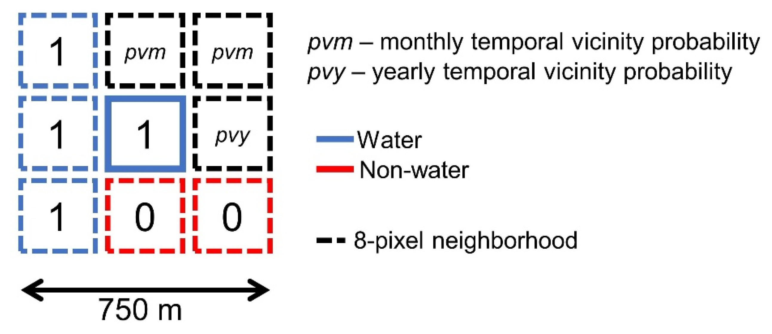
2.2.2. Temporal Vicinity Probability

To consider more short-term changes, the yearly and monthly temporal vicinity of each pixel is evaluated. Whereas the monthly timeframe covers a rather small number of temporal neighbors {t ∈ ℤ|−15 ≤ t ≤ 15}, yearly estimates focus on the behavior of a complete annual cycle {t ∈ ℤ|−182 ≤ t ≤ 182}. A two-band layer is generated for each defined temporal vicinity (31 days and 365 days) using Equation (3) to estimate water probability (month pvm, year pvy) and Equation (4) for the corresponding reliability (month rvm, year rvy). An example for the theoretical consideration of an 8-day past/future vicinity is given in Figure 4.
In case the temporal investigation extent is not covered by the available time series data, additional days are added to the past or future vicinity. Thus, the same amount of information is considered for all estimates. If no valid observation can be found in the aspired timeframe, the layer states “no data” and reliability equals zero. This results in a daily output of vicinity layer information.

2.2.3. Seasonal Probability

Waterbodies typically exhibit seasonally dependent extent changes. This behavior is captured by the seasonal probability layer (ps) by investigating the state of a pixel at a specified time in every available year of the time series. Therefore, the monthly temporal vicinity probability (pvm) of a certain day of the year (DOY) of every complete year within the input time series is considered (Figure 5).
Consequently, the typical seasonal state of a pixel is revealed. Pixelwise processing of seasonal probability and reliability (rs) is achieved by considering the total number of investigated years (N) and the number of valid years (Nvalid) for which a valid estimate pvmy at the evaluated DOY is available:
p s = y = 1 N p v m y ( D O Y ) N v a l i d
r s = N v a l i d N
Only with a sufficient amount of observed temporally connected years, it is possible to describe seasonal characteristics accurately. As a result, seasonal layer estimates are provided once for every DOY.

2.2.4. Spatial Neighborhood Probability

Water naturally accumulates to larger coherent waterbodies on the surface. Due to this spatial relationship, a pixel that has a relatively high number of water-covered neighbors is more likely to contain water itself. This relationship can be quantified by considering the 8-pixel neighborhood of an evaluation pixel in the center (Figure 6).
To estimate neighborhood probability (pn) and reliability (rn), the respective probabilities (pi) and reliabilities (ri) of all n valid pixels in the neighborhood, as well as the center pixel, are averaged:
p n = i = 1 9 p i n
r n = i = 1 9 r i n
Hereby, valid water or non-water observations contribute with 100% or 0% probability, respectively. In case of invalid observations, primarily, the monthly temporal vicinity layer (pvm, rvm) is employed. Alternatively, annual temporal vicinity estimates (pvy, rvy) substitute monthly estimates in case they render “no data.” If no valid estimate is found in both temporal vicinity layers, the pixel is disregarded for calculation.
p i = { 100 % 0 % p v m ,   p v y   if   water   observation if   non - water   observation else ,   if   available
r i = { 100 % r v m , r v y if   valid   observation else ,   if   available  

2.2.5. Temporally Closest-Observation-Based Probability

Pixel states of the temporally closest valid observations constitute the most short-term information available. We estimated probability and reliability (pc, rc) by considering the closest valid time series observations (e.g., t−1 and t3 in Figure 4) in an ROI-specific search window. This window is defined by the pixel variabilities given by the long-term layer Va band. By considering the mean variability of pixels that at least changed once (Va > 0), the average number of days until a state change occurs (d) is determined. The search window extent (ts) in which the days of closest past and future observations are identified, is defined according to {ts ∈ ℤ|−dts ≤ d}. The information of the two temporally closest detected pixel states (DWcpast, DWcfuture) is combined with respect to their temporal distance to the evaluation day (tc), in order to yield a water probability estimate:
p c = D W c p a s t w p a s t + D W c f u t u r e w f u t u r e w p a s t + w f u t u r e
with
w = 1 | t c |  
Thus, pc only deviates from 0% or 100% if the past and future closest observations display opposite states. The reliability of these estimates (rc) is given by the number of invalid observations (IO) until the closest valid observations, relative to the total number of possible invalid observations within the search window:
r c = 1 I O ( d 2 ) 2
Consequently, direct valid temporal neighbors result in 100% reliability, whereas the closest valid observations on the edge of the search window produces 0% reliability. In case no past and future observations are found within the search window, the pixel is disregarded due to a lack of temporal coherence.

2.2.6. Combination of Temporal Probability Layers

Each of the presented temporal probability layers concentrates on specific spatiotemporal characteristics. To combine their information, a single temporal probability estimate (pt) is generated. Therefore, the weighted arithmetic mean function is used to aggregate the previously established probabilities by considering their respective reliabilities as weights:
p t = p l r l + p v y r v y + p v m r v m + p s r s + p n r n + p c r c r l + r v y + r v m + r s + r n + r c
As a result, the reliability of a pixel probability estimate determines its contribution to the combined daily outcome.

3. Results

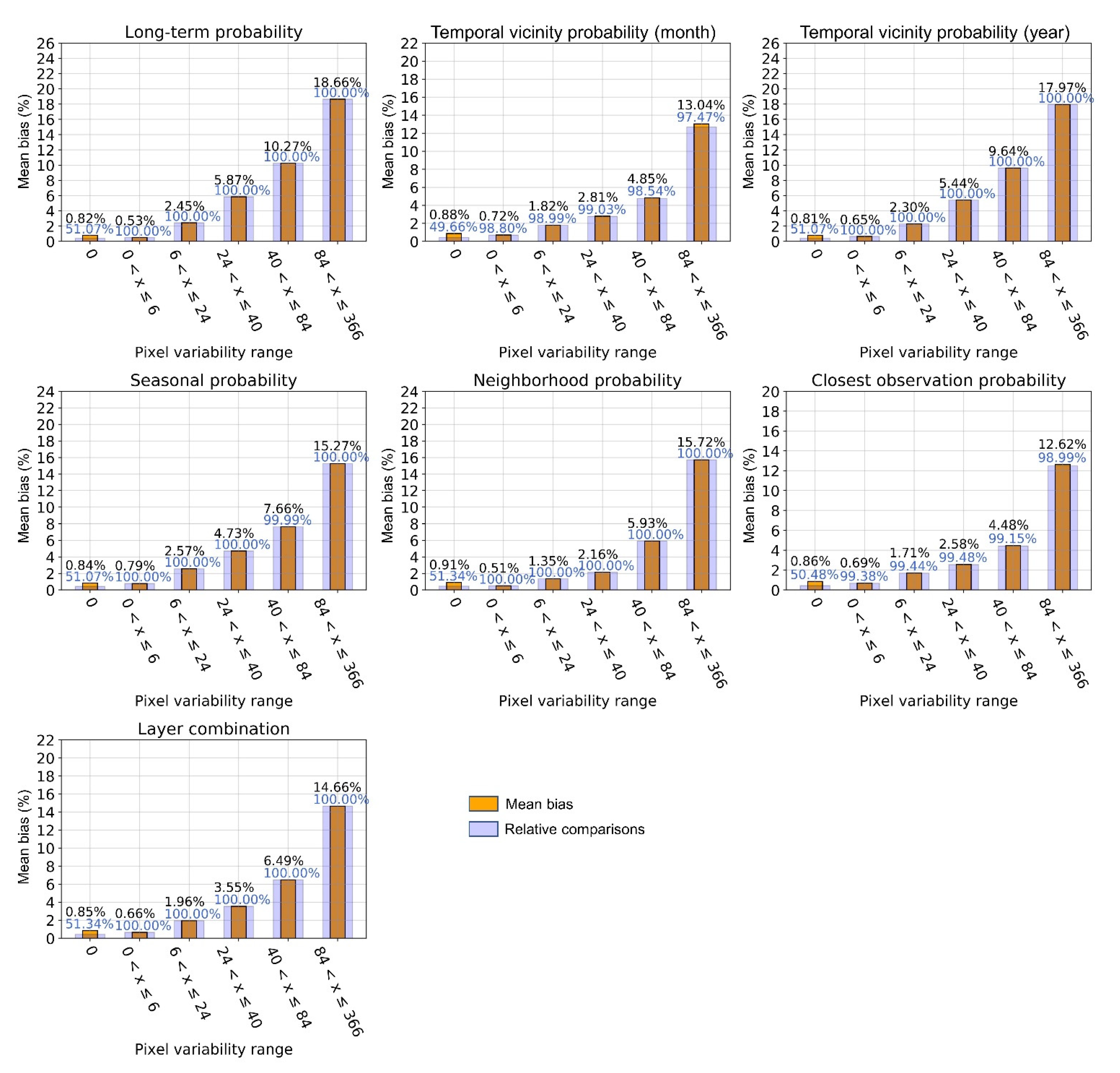
3.1. Evaluation of Temporal Probability Layers

We introduced a total of 788,832 artificial gaps (invalid observations) to the original time series of four test ROIs (Figure 2) by following a stratification strategy based on variability percentiles. Temporal layer generation on these manipulated time series enabled a subsequent assessment. To account for different behavioral-types of pixels, the gapping process is structured with reference to long-term pixel variability (Va). Based on the number of pixel state changes throughout the time series, percentiles are determined to create specific evaluation ranges for each test ROI. As most areas within a test ROI are constituted by permanent non-water surface, the majority of pixels are allocated to the zero-variability percentile. However, only unique percentiles were chosen as limits for evaluation ranges, with each representing one percent of the MODIS tile data (except the zero-variability range). Accordingly, unique sets of evaluation ranges are determined per test ROI. Pixels contained in the determined evaluation ranges for ROI h18v03 are shown in Figure 7.
As temporal layer generation is sensitive to invalid observations and the pixel state change frequency, an evaluation in variability ranges provides detailed insight into layer performance. Stratifying artificial gaps according to data percentiles also ensures that the gapping process does not excessively interfere with the true nature of the original time series. We randomly introduced two gaps per day and evaluation range. For an ROI, this results in a total of 7304 gaps per evaluation range. The absolute differences of temporal probability estimates and detected (gapped) states were calculated to yield the mean bias for each evaluation range. The results of test ROI h18v03 are shown in Figure 8.
Despite differing evaluation variability ranges of the specific ROIs, results showed similar patterns in all four test sites. With increasing variability, layers that focused on more immediate temporal windows for probability estimation (month-vicinity-, neighborhood- and closest-observation-based probability) had lower bias than long-term-, year-vicinity- and seasonal-probability layers, as well as the combined layer. For relatively static pixels (low variability), better performance was observed for layers considering larger temporal windows. The most challenging test site regarding layer performance was test ROI h18v03 (Figure 7 and Figure 8), as it features considerable cloud coverage and various water variability patterns. Temporal layer performances regarding the highest pixel variability range (variability ≥ 99th percentile) for all test ROIs are shown in Table 1.
Results in all four test ROIs indicate, that temporal layer combination (pt) can determine the true state with >90% accuracy on average in the challenging circumstances of high pixel variability.

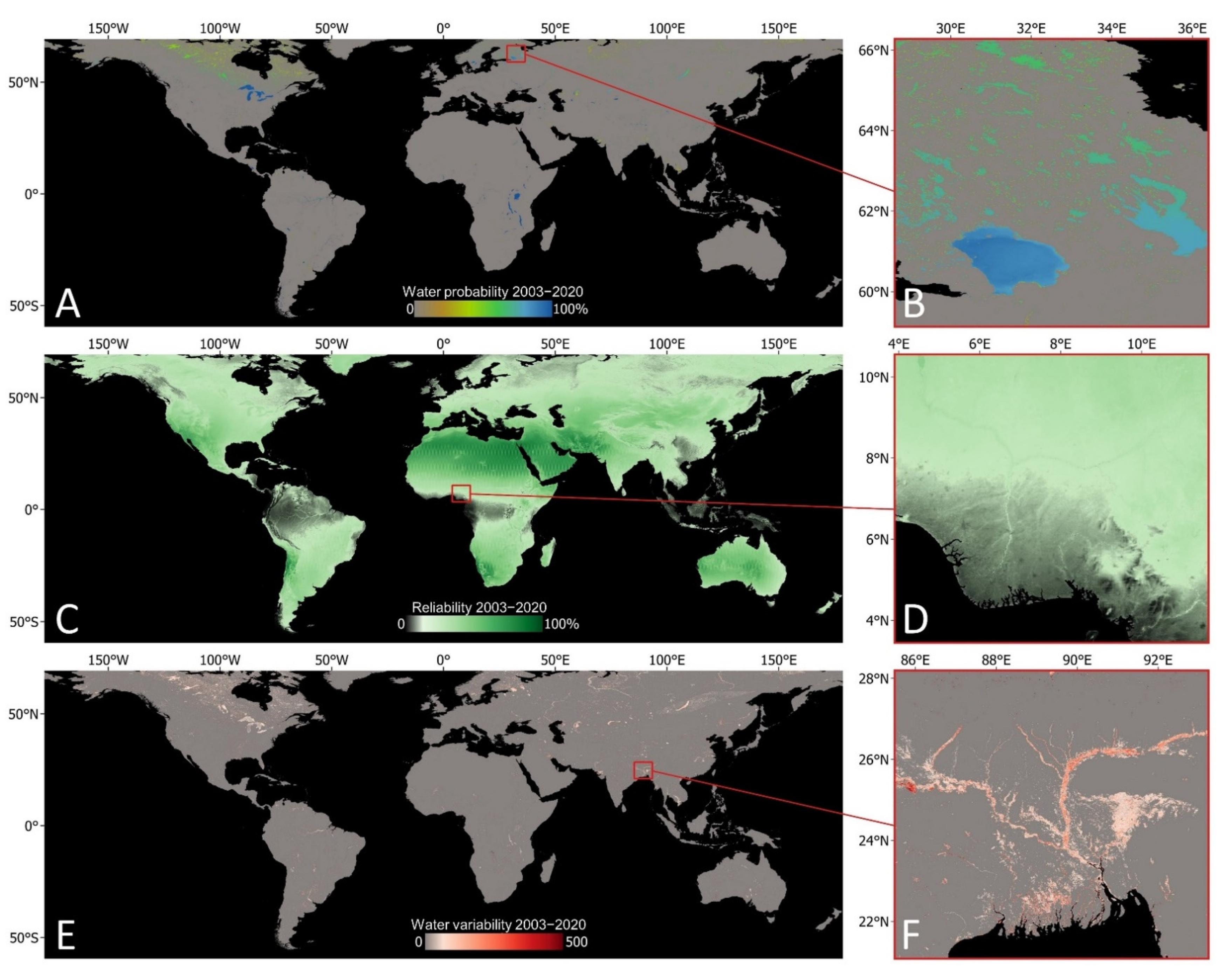
3.2. Global Uncertainty Maps

Utilizing the full spatiotemporal range of the GWP product, we generated global maps based on 6574 days of data (2003–2020). Accordingly, comprehensive uncertainty-related information regarding the product is given by the spatial distribution of long-term probability (pl), reliability (rl) and variability (Va) (Figure 9).
The global water probability map (Figure 9A,B) indicates how often a pixel was classified as water, considering only valid observations. Therefore, a high water probability of 95–100% represents relatively permanent water pixels, which account for 0.53% of the data. The majority of data (97.03%) consists of zero probability pixels, depicting permanent non-water areas. Other probability ranges suggest that surface water has been present for a limited amount of time, or exhibits reoccurrence patterns (e.g., due to seasonal lake ice; Figure 9B). The map of global reliability (Figure 9C,D) shows how many valid observations are available per pixel to detect water and non-water states. Accordingly, water probability estimates for areas with high reliability are based on a larger data background. This is mostly the case for regions with low cloud coverage (e.g., arid desert regions; see also Figure 2). On the other hand, estimates with low reliability are mainly found in the tropics (convective clouds), but also in regions that commonly feature orographic clouds (e.g., northern Andes). The degree to which pixels are subject to water/non-water state changes is shown by the water variability map (Figure 9E,F). Such pixels are typically located along coastlines of surface water bodies and rivers, or flood-prone areas (e.g., Monsoon flooding in the Ganges–Brahmaputra estuary; Figure 9F).

4. Discussion

Evaluation results based on the artificial gapping of the surface water time series of four test ROIs showed similar layer performance patterns for all study sites. As we stratified artificial gaps according to water variability, probability layer performance mainly depended on the water permanence type. Accordingly, pixels with lower variability (more constant pixels) generally showed smaller mean bias to probability layer estimates than pixels with higher variability. Layers concentrating on closer temporal neighbors by utilizing smaller temporal windows (short-term-oriented) showed better performance for change-intensive pixels (Table 1). For relatively constant pixels, long-term-oriented (≥1 year) probability layers performed only slightly better than short-term-oriented layers. This suggests that short-term-focused layers are generally more suitable for the prediction of unknown surface water states based on time series information. Considering all presented temporal characteristics of surface water, as well as reliability related to data availability, the combined temporal probability layer offers a good compromise for broad application. With an overall mean bias of 3.45% in our evaluation experiments, this layer is able to accurately quantify temporal uncertainty of surface water time series.
The global and long-term applicability of our approach was demonstrated by the generation of global uncertainty maps featuring long-term probability, reliability and variability. With this information, it is possible to assess the likelihood of surface water occurrence, data availability and water/non-water change characteristics for a given surface water time series dataset.

4.1. Potential and Limitations of Single Probability Layers

Generally, the long-term layer (pl, rl, Va) is the most comprehensive probability layer, as all available temporal information is condensed in one raster composite (Figure 9). This helps to characterize typical surface water behavior and provides guidance on which probability layer is suitable for the prediction of invalid observations. For instance, in regions with low reliability, an emphasis on layers that feature larger temporal windows (e.g., a long-term or yearly temporal vicinity layer) can prove beneficial. On the other hand, given high reliability and variability, a focus on short-term information (e.g., temporally closest observations) should be preferred. Moreover, reliability and variability play an important role in the anticipation of the magnitude of temporal uncertainties regarding an ROI. Accordingly, long-term reliability reveals actual data availability in a region, offering an overview on data gap characteristics. In case of high long-term variability, larger uncertainties have to be expected for invalid observations (additional aleatoric uncertainty). Accordingly, layer evaluation showed that long-term probability is more suitable for estimating pixels featuring low variability (Figure 8).
Two temporal vicinity layers facilitate the assessment of specific temporal windows on a daily basis. In our study, we focused on monthly (pvm, rvm) and yearly (pvy, rvy) intervals. The probability regarding intermittent monthly observations showed good overall performance for capturing surface water behavior. The larger yearly window, which is intended to capture surface water dynamics influenced by all occurring seasonal effects, performs well mainly in low variability ranges. Nonetheless, for regions with extensive data gaps exceeding one month, the yearly layer provides a stable substitute for more short-term estimates.
To capture the seasonal characteristics of surface water in particular, the seasonal layer (ps, rs) provides probability for reoccurring water coverage (of a pixel) in a monthly time window. As most surface waterbodies exhibit seasonal extent changes, this layer shows adequate performance. Emphasis on this layer may be given if prior knowledge of distinct seasonal behavior of surface water is at hand or the focus of the investigation.
The neighborhood layer (pn, rn) combines current or (if not available) temporal vicinity information of a center pixel and its eight-pixel neighborhood. As a result, daily estimates regarding the probability that a pixel is part of a larger coherent waterbody are provided. This also promotes inferences on partial water coverage, as non-water pixels adjacent to water pixels have a higher chance of containing water fragments themselves. Conversely, the same principle is applicable for water pixels neighboring non-water pixels. Performance evaluation revealed that neighborhood probability estimates perform best (in comparison) for pixels featuring medium variability (Figure 8). Furthermore, relatively high (>95%) or low (<5%) neighborhood probability, in combination with high reliability, indicates complete water or non-water coverage of a pixel, respectively.
Utilizing the temporally closest information available, the closest observation-based layer (pc, rc) outperforms other layers for pixels with high variability (Table 1). This becomes beneficial when water coverage is prone to frequent short-term changes (high variability). Since this layer is only based on two observations, misclassifications can have a strong impact on its accuracy. This also applies if the temporal distance to closest temporal observations is large (indicated by the corresponding reliability).

4.2. Uncertainty Quantification

Outcomes of the presented methodologies are probabilistic estimates at pixel-level. Water probability in a temporal context provides information on the likelihood that a pixel is covered by water in case it cannot be observed directly. Consequently, the validity of total surface water extent, which is also based on interpolated pixels, can be assessed. For the conversion to areal uncertainty values, probabilities can be utilized to define the relative amount of the total pixel area that can be regarded as uncertain. By aggregating this information for a selection of pixels (ROI), the corresponding uncertainty can be quantified. The resulting temporal error ranges determine the uncertainty span in which the true water extent can be assumed, considering lack of knowledge due to invalid observations. Furthermore, the reliability band allows for the evaluation of probability estimates, as well as the actual data availability for specific study sites.

4.3. Alternative Applications and Extension to Other Time Series Datasets

Generated layer estimates are provided for every pixel of an image, independent of valid or invalid observations. Thus, valid observation pixels showing distinct diversity of classification outcome and specific probability estimate can be identified. This enables the systematic investigation of potential misclassifications or unexpected classifications. Furthermore, layer estimates are suitable for a probabilistic interpolation of data gaps. Other studies utilized temporal information inherent to a geospatial time series dataset primarily outside uncertainty-related context. For instance, Pekel et al. [36] generated a global surface water dataset based on the Landsat data archive spanning over more than 32 years. Hereby, temporal information was involved in the classification procedure, the generation of thematic maps and the identification of temporal water types and their transitions. Similarly, Mueller et al. [37] used the frequency of detected water to determine temporal water types. Pickens et al. [38] utilized temporal information from Landsat time series for quantifying the extent and change dynamics of global inland surface water. Additionally, they used standard errors based on reference samples to comprehensively quantify the associated uncertainties of areal estimates.
Many widely used Earth observation variables (e.g., normalized difference vegetation index (NDVI), leaf area index (LAI), soil moisture, burned area, snow cover) exhibit distinct spatiotemporal characteristics. Layer development in this study is focused on the specific target variable of surface water. To optimize method application and layer performance for different target variables, relevant spatiotemporal characteristics (e.g., length of temporal windows or spatial connection) have to be considered. For non-binary variables (e.g., NDVI, LAI), normalization to values ranging from 0 to 1 is required for a straightforward implementation of the proposed probability-based methodology.

4.4. Limitations

Limitations of temporal uncertainty estimation are given by the temporal resolution. For example, compared to MODIS (daily revisit times of two sensors), Landsat sensor imagery exhibits a significantly lower temporal resolution (~16-day revisit period coupled with cloud contamination). Consequently, derived temporal uncertainty has to be interpreted in a different context, as important dynamics might be missed [39,40]. If information is generated with a detail level that is not sustained by data availability, uncertainty increases due to sampling errors.
Layer performance mainly depends on two factors: data variability and reliability. In case of high variability but low reliability, the quality of probabilistic estimates decreases. Moreover, in case of low reliability, the accurate determination of variability is limited. This can lead to an incorrect assessment of study regions if limitations given by the data are not considered.

5. Conclusions

The demand for a comprehensive understanding of planet-wide processes drives the need for global Earth observation time series. Users of respective data products are often unaware of inherent uncertainty, as it is not sufficiently communicated. Many time series datasets rely on interpolation methods, making temporal interpolation uncertainty an essential characteristic. To fully comprehend the validity and limitations of data applications, it is imperative to consider the sensitivity to uncertainties. For geospatial data, this means locating and quantifying uncertainties spatially and temporally in order to ensure data quality.
We demonstrated a systematic approach to accurately quantify the temporal uncertainties of a global surface water time series. Seven temporal layers featuring probability and reliability at pixel-level were derived from time series-inherent information. This enables the straightforward provision of uncertainties alongside a product’s global and daily spatiotemporal resolution. Layers are designed to characterize specific surface water behavior. Hereby, temporal and spatial aspects were considered. Accordingly, we chose temporal intervals to characterize long-term behavior (long-term probability), natural reoccurring events (year-vicinity- and seasonal-probability) and sporadic behavior (month-vicinity-, neighborhood- and closest-observation-based probability), which may occur due to extreme weather events (e.g., floods, droughts), or human interaction (e.g., dams, irrigation). Focus on distinct layers may be appropriate, depending on prior knowledge of the study area (e.g., typical behavior of the target variable), data usage (e.g., processing capabilities) or scientific question (e.g., interest in seasonal dynamics). Otherwise, various aspects of temporal information contained in the time series should be considered. With an emphasis on layer reliability, the combined temporal probability layer fulfills this requirement. As a result, users of the GWP product are able to benefit from different types of temporal uncertainty information. A detailed performance analysis was conducted for 788,832 artificial data gaps in four test regions. Hereby, the potentials of single layers and their combination were outlined.
Extensive uncertainty maps were generated by processing 6574 days (2003–2020) of global-scale data. Hereby, the ability to evaluate comprehensive spatiotemporal time series information was demonstrated, and important characteristics of the global product were revealed. By applying the proposed methodology, temporal uncertainty of manifold geospatial time series products can be quantified. As a result, the validity of the results obtained through time series datasets can be improved. This becomes especially relevant for the development and calibration of models driven by respective data. Furthermore, time series accompanied by uncertainty layers at pixel-level allow for a more critical view on spatiotemporal data patterns. Consequently, a foundation for sound scientific conclusions and rational decision making is provided.

Author Contributions

S.M. developed the initial research design. C.K., I.K. and M.R. provided guidance on the research content, manuscript structure and suggested figures. S.M. and I.K. performed the literature research. S.M. wrote the manuscript and designed the figures. All authors contributed to the final version of the manuscript via intensive discussions and working over consecutive versions of the text and figures. All authors have read and agreed to the published version of the manuscript.

Funding

This research was funded by the DFG (Deutsche Forschungsgemeinschaft) GlobalCDA (Global Calibration and Data Assimilation) project.

Institutional Review Board Statement

Not applicable.

Informed Consent Statement

Not applicable.

Data Availability Statement

The data presented in this study are available on request from the corresponding author.

Conflicts of Interest

The authors declare no conflict of interest.

References

  1. Global Climate Observing System (GCOS). Monitoring Principles. Available online: https://gcos.wmo.int/en/essential-climate-variables/about/gcos-monitoring-principles (accessed on 17 August 2021).
  2. Kavvada, A.; Metternicht, G.; Kerblat, F.; Mudau, N.; Haldorson, M.; Laldaparsad, S.; Friedl, L.; Held, A.; Chuvieco, E. Towards Delivering on the Sustainable Development Goals Using Earth Observations. Remote Sens. Environ. 2020, 247, 111930. [Google Scholar] [CrossRef]
  3. Kansakar, P.; Hossain, F. A Review of Applications of Satellite Earth Observation Data for Global Societal Benefit and Stewardship of Planet Earth. Space Policy 2016, 36, 46–54. [Google Scholar] [CrossRef]
  4. Mayr, S.; Kuenzer, C.; Gessner, U.; Klein, I.; Rutzinger, M. Validation of Earth Observation Time-Series: A Review for Large-Area and Temporally Dense Land Surface Products. Remote Sens. 2019, 11, 2616. [Google Scholar] [CrossRef] [Green Version]
  5. Serrat-Capdevila, E.M.C.D.A. Challenges of Remote Sensing Validation. In Earth Observation for Water Resources Management: Current Use and Future Opportunities for the Water Sector; The World Bank: Washington, DC, USA, 2016; pp. 167–171. ISBN 978-1-4648-0475-5. [Google Scholar]
  6. Kuenzer, C.; Dech, S.; Wagner, W. Remote Sensing Time Series; Springer International Publishing: Basel, Switzerland, 2015; Volume 22. [Google Scholar]
  7. Kuenzer, C.; Ottinger, M.; Wegmann, M.; Guo, H.; Wang, C.; Zhang, J.; Dech, S.; Wikelski, M. Earth Observation Satellite Sensors for Biodiversity Monitoring. Int. J. Remote Sens. 2014, 35, 6599–6647. [Google Scholar] [CrossRef] [Green Version]
  8. Campbell, J.B. Introduction to Remote Sensing, 3rd ed.; Guilford Press: New York, NY, USA, 2002; ISBN 1-57230-640-8. [Google Scholar]
  9. Klein, I.; Gessner, U.; Dietz, A.J.; Kuenzer, C. Global WaterPack–A 250 m Resolution Dataset Revealing the Daily Dynamics of Global Inland Water Bodies. Remote Sens. Environ. 2017, 198, 345–362. [Google Scholar] [CrossRef]
  10. Liu, Y. Why NDWI Threshold Varies in Delineating Water Body from Multitemporal Images? In Proceedings of the 2012 IEEE International Geoscience and Remote Sensing Symposium, Munich, Germany, 22–27 July 2012; IEEE: Munich, Germany, 2012; pp. 4375–4378. [Google Scholar]
  11. Kutser, T.; Vahtmäe, E.; Praks, J. A Sun Glint Correction Method for Hyperspectral Imagery Containing Areas with Non-Negligible Water Leaving NIR Signal. Remote Sens. Environ. 2009, 113, 2267–2274. [Google Scholar] [CrossRef]
  12. Ticehurst, C.; Guerschman, J.P.; Chen, Y. The Strengths and Limitations in Using the Daily MODIS Open Water Likelihood Algorithm for Identifying Flood Events. Remote Sens. 2014, 19, 11791–11809. [Google Scholar] [CrossRef] [Green Version]
  13. Kumar, C.; Podestá, G.; Kilpatrick, K.; Minnett, P. A Machine Learning Approach to Estimating the Error in Satellite Sea Surface Temperature Retrievals. Remote Sens. Environ. 2021, 255, 112227. [Google Scholar] [CrossRef]
  14. Brown, M.E.; Pinzon, J.E.; Didan, K.; Morisette, J.T.; Tucker, C.J. Evaluation of the Consistency of Long-Term NDVI Time Series Derived from AVHRR, SPOT-Vegetation, SeaWiFS, MODIS, and Landsat ETM+ Sensors. IEEE Trans. Geosci. Remote Sens. 2006, 44, 1787–1793. [Google Scholar] [CrossRef]
  15. Lei, F.; Crow, W.T.; Shen, H.; Su, C.-H.; Holmes, T.R.H.; Parinussa, R.M.; Wang, G. Assessment of the Impact of Spatial Heterogeneity on Microwave Satellite Soil Moisture Periodic Error. Remote Sens. Environ. 2018, 205, 85–99. [Google Scholar] [CrossRef]
  16. Verger, A.; Baret, F.; Weiss, M. A Multisensor Fusion Approach to Improve LAI Time Series. Remote Sens. Environ. 2011, 115, 2460–2470. [Google Scholar] [CrossRef] [Green Version]
  17. Weiss, D.J.; Atkinson, P.M.; Bhatt, S.; Mappin, B.; Hay, S.I.; Gething, P.W. An Effective Approach for Gap-Filling Continental Scale Remotely Sensed Time-Series. ISPRS J. Photogramm. Remote Sens. Off. Publ. Int. Soc. Photogramm. Remote Sens. ISPRS 2014, 98, 106–118. [Google Scholar] [CrossRef] [PubMed] [Green Version]
  18. Zhou, J.; Jia, L.; Menenti, M.; Gorte, B. On the Performance of Remote Sensing Time Series Reconstruction Methods–A Spatial Comparison. Remote Sens. Environ. 2016, 187, 367–384. [Google Scholar] [CrossRef]
  19. Zhou, J.; Jia, L.; Menenti, M. Reconstruction of Global MODIS NDVI Time Series. Remote Sens. Environ. 2015, 163, 217–228. [Google Scholar] [CrossRef]
  20. Fang, H.; Liang, S.; Townshend, J.; Dickinson, R. Spatially and Temporally Continuous LAI Data Sets Based on an Integrated Filtering Method. Remote Sens. Environ. 2008, 112, 75–93. [Google Scholar] [CrossRef]
  21. Gerber, F.; de Jong, R.; Schaepman, M.E.; Schaepman-Strub, G.; Furrer, R. Predicting Missing Values in Spatio-Temporal Remote Sensing Data. IEEE Trans. Geosci. Remote Sens. 2018, 56, 2841–2853. [Google Scholar] [CrossRef] [Green Version]
  22. Abolafia-Rosenzweig, R.; Pan, M.; Zeng, J.L.; Livneh, B. Remotely Sensed Ensembles of the Terrestrial Water Budget over Major Global River Basins: An Assessment of Three Closure Techniques. Remote Sens. Environ. 2020, 252, 112191. [Google Scholar] [CrossRef]
  23. Bayat, B.; Camacho, F.; Nickeson, J.; Cosh, M.; Bolten, J.; Vereecken, H.; Montzka, C. Toward Operational Validation Systems for Global Satellite-Based Terrestrial Essential Climate Variables. Int. J. Appl. Earth Obs. Geoinf. 2021, 95, 102240. [Google Scholar] [CrossRef]
  24. Pasetto, D.; Arenas-Castro, S.; Bustamante, J.; Casagrandi, R.; Chrysoulakis, N.; Cord, A.F.; Dittrich, A.; Domingo-Marimon, C.; El Serafy, G.; Karnieli, A.; et al. Integration of Satellite Remote Sensing Data in Ecosystem Modelling at Local Scales: Practices and Trends. Methods Ecol. Evol. 2018, 9, 1810–1821. [Google Scholar] [CrossRef] [Green Version]
  25. Schneider, K.; Mauser, W. Using Remote Sensing Data to Model Water, Carbon, and Nitrogen Fluxes with PROMET-V; Owe, M., D’Urso, G., Zilioli, E., Eds.; International Society for Optics and Photonics: Barcelona, Spain, 2001; pp. 12–23. [Google Scholar]
  26. Calvet, J.-C.; de Rosnay, P.; Penny, S.G. Editorial for the Special Issue “Assimilation of Remote Sensing Data into Earth System Models”. Remote Sens. 2019, 11, 2177. [Google Scholar] [CrossRef] [Green Version]
  27. Boschetti, L.; Roy, D.P.; Giglio, L.; Huang, H.; Zubkova, M.; Humber, M.L. Global Validation of the Collection 6 MODIS Burned Area Product. Remote Sens. Environ. 2019, 235, 111490. [Google Scholar] [CrossRef] [PubMed]
  28. Papa, F.; Prigent, C.; Aires, F.; Jimenez, C.; Rossow, W.B.; Matthews, E. Interannual Variability of Surface Water Extent at the Global Scale, 1993–2004. J. Geophys. Res. 2010, 115, D12111. [Google Scholar] [CrossRef]
  29. Carroll, M.L.; Townshend, J.R.; DiMiceli, C.M.; Noojipady, P.; Sohlberg, R.A. A New Global Raster Water Mask at 250 m Resolution. Int. J. Digit. Earth 2009, 2, 291–308. [Google Scholar] [CrossRef]
  30. Carroll, M.L.; DiMiceli, C.M.; Townshend, J.R.G.; Sohlberg, R.A.; Elders, A.I.; Devadiga, S.; Sayer, A.M.; Levy, R.C. Development of an Operational Land Water Mask for MODIS Collection 6, and Influence on Downstream Data Products. Int. J. Digit. Earth 2016, 10, 207–218. [Google Scholar] [CrossRef]
  31. D’Odorico, P.; Gonsamo, A.; Pinty, B.; Gobron, N.; Coops, N.; Mendez, E.; Schaepman, M.E. Intercomparison of Fraction of Absorbed Photosynthetically Active Radiation Products Derived from Satellite Data over Europe. Remote Sens. Environ. 2014, 142, 141–154. [Google Scholar] [CrossRef]
  32. Dorigo, W.A.; Xaver, A.; Vreugdenhil, M.; Gruber, A.; Hegyiová, A.; Sanchis-Dufau, A.D.; Zamojski, D.; Cordes, C.; Wagner, W.; Drusch, M. Global Automated Quality Control of In Situ Soil Moisture Data From The International Soil Moisture Network. Vadose Zone J. 2013, 12, 1–21. [Google Scholar] [CrossRef]
  33. Wang, D.; Liang, S. Improving LAI Mapping by Integrating MODIS and CYCLOPES LAI Products Using Optimal Interpolation. IEEE J. Sel. Top. Appl. Earth Obs. Remote Sens. 2014, 7, 445–457. [Google Scholar] [CrossRef]
  34. Lehner, B.; Döll, P. Development and Validation of a Global Database of Lakes, Reservoirs and Wetlands. J. Hydrol. 2004, 296, 1–22. [Google Scholar] [CrossRef]
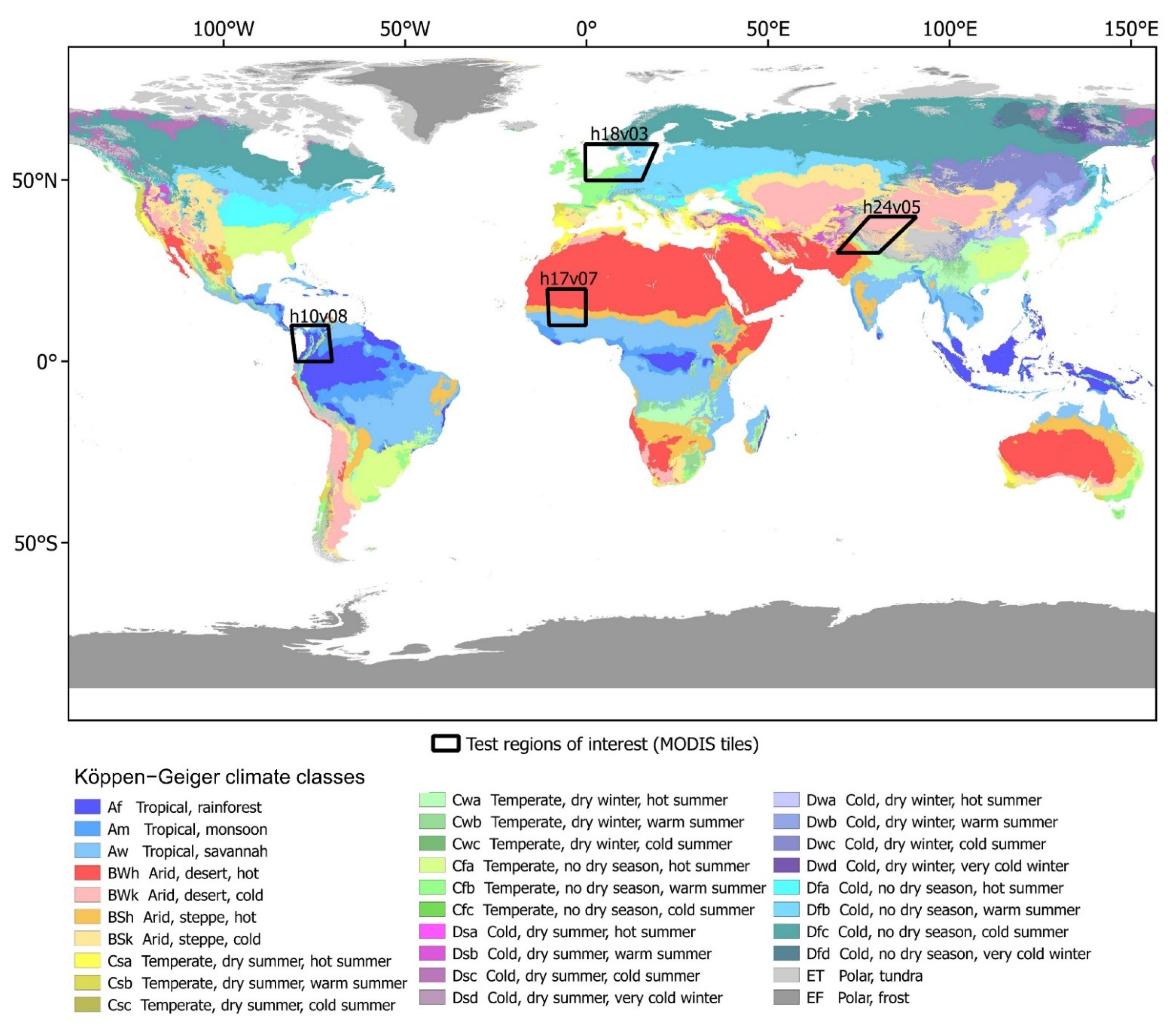
  35. Beck, H.E.; Zimmermann, N.E.; McVicar, T.R.; Vergopolan, N.; Berg, A.; Wood, E.F. Present and Future Köppen-Geiger Climate Classification Maps at 1-Km Resolution. Sci. Data 2018, 5, 180214. [Google Scholar] [CrossRef] [PubMed] [Green Version]
  36. Pekel, J.-F.; Cottam, A.; Gorelick, N.; Belward, A.S. High-Resolution Mapping of Global Surface Water and Its Long-Term Changes. Nature 2016, 540, 418–422. [Google Scholar] [CrossRef] [PubMed]
  37. Mueller, N.; Lewis, A.; Roberts, D.; Ring, S.; Melrose, R.; Sixsmith, J.; Lymburner, L.; McIntyre, A.; Tan, P.; Curnow, S.; et al. Water Observations from Space: Mapping Surface Water from 25 Years of Landsat Imagery across Australia. Remote Sens. Environ. 2016, 174, 341–352. [Google Scholar] [CrossRef] [Green Version]
  38. Pickens, A.H.; Hansen, M.C.; Hancher, M.; Stehman, S.V.; Tyukavina, A.; Potapov, P.; Marroquin, B.; Sherani, Z. Mapping and Sampling to Characterize Global Inland Water Dynamics from 1999 to 2018 with Full Landsat Time-Series. Remote Sens. Environ. 2020, 243, 111792. [Google Scholar] [CrossRef]
  39. Ling, F.; Li, X.; Foody, G.M.; Boyd, D.; Ge, Y.; Li, X.; Du, Y. Monitoring Surface Water Area Variations of Reservoirs Using Daily MODIS Images by Exploring Sub-Pixel Information. ISPRS J. Photogramm. Remote Sens. 2020, 168, 141–152. [Google Scholar] [CrossRef]
  40. Li, L.; Skidmore, A.; Vrieling, A.; Wang, T. A New Dense 18-Year Time Series of Surface Water Fraction Estimates from MODIS for the Mediterranean Region. Hydrol. Earth Syst. Sci. 2019, 23, 3037–3056. [Google Scholar] [CrossRef] [Green Version]
Figure 1. Global WaterPack (GWP) application to monitor the surface water decline of Lake Urmia from 2003–2016. Grey areas refer to the Global Lakes and Wetlands Database (GLWD) [34].
Remotesensing 13 03454 g001
Figure 2. Selected test ROIs for layer evaluation and climate classes [35].
Remotesensing 13 03454 g002
Figure 3. Combination of MODIS sensor information from Aqua and Terra satellites into a time series of two binary arrays. Binary assessment: 1 ≙ true and 0 ≙ false.
Remotesensing 13 03454 g003
Figure 4. Pixel representation of temporal neighbors in the past and future vicinity. Here, an 8-day past/future vicinity is considered and water probability for the evaluated pixel would be 2/3 with a reliability of 3/9. Binary assessment: 1 ≙ true and 0 ≙ false.
Remotesensing 13 03454 g004
Figure 5. Seasonal probability on pixel-level by considering water reoccurrence on a specific day of the year. Binary assessment: 1 ≙ true and 0 ≙ false.
Remotesensing 13 03454 g005
Figure 6. Example of the pixel neighborhood used for probability estimation. Here, three observations are invalid and, therefore, they are substituted using temporal vicinity estimates (pvm, pvy). Binary assessment: 1 ≙ true and 0 ≙ false.
Remotesensing 13 03454 g006
Figure 7. Evaluation ranges according to pixel variabilities (water/non-water state changes) over 3652 days (2010–2019) for test ROI h18v03: (A) complete ROI tile (1:8,500,000), (B) zoomed-in tile (1:650,000), (C) higher-resolution Landsat 8 true color image (1:650,000), and (D) zoomed-in Lake Müritz (1:86,000).
Remotesensing 13 03454 g007
Figure 8. Evaluation results for temporal probability layers of test ROI h18v03. The blue bars show the ratio of potential comparisons (7304) to possible comparisons (layer estimate ≠ “no data”).
Remotesensing 13 03454 g008
Figure 9. Global long-term water probability (A,B), reliability (C,D) and variability (E,F) for the years 2003–2020.
Remotesensing 13 03454 g009
Table 1. Mean bias of temporal layers regarding the highest variability evaluation range for each test ROI.
LayerTile h10v08Tile h17v07Tile h18v03Tile h24v05
Long-term probability (pl)13.98%8.28%18.66%13.67%
Year vicinity probability (pvy)9.32%7.50%17.97%12.00%
Month vicinity probability (pvm)6.75%2.93%13.04%5.69%
Seasonal probability (ps)13.63%5.14%15.27%10.20%
Neighborhood probability (pn)6.83%2.89%15.72%5.31%
Closest observation probability (pc)6.88%2.63%12.62%4.73%
Combined temporal probability (pt)9.31%4.42%14.66%7.82%
Publisher’s Note: MDPI stays neutral with regard to jurisdictional claims in published maps and institutional affiliations.

