Article

An Entropy-Weighting Method for Efficient Power-Line Feature Evaluation and Extraction from LiDAR Point Clouds

1
College of Earth Sciences, Chengdu University of Technology, Chengdu 610059, China
2
Faculty of Geomatics, East China University of Technology, Nanchang 330013, China
3
Chengdu Alundar Technology Co., Ltd., Chengdu 610041, China
*
Author to whom correspondence should be addressed.
Remote Sens. 2021, 13(17), 3446; https://doi.org/10.3390/rs13173446
Submission received: 11 July 2021 / Revised: 19 August 2021 / Accepted: 27 August 2021 / Published: 30 August 2021
(This article belongs to the Special Issue Remote Sensing for Power Line Corridor Surveys)

Abstract

:
Power-line inspection is an important means to maintain the safety of power networks. Light detection and ranging (LiDAR) technology can provide high-precision 3D information about power corridors for automated power-line inspection, so there are more and more utility companies relying on LiDAR systems instead of traditional manual operation. However, it is still a challenge to automatically detect power lines with high precision. To achieve efficient and accurate power-line extraction, this paper proposes an algorithm using entropy-weighting feature evaluation (EWFE), which is different from the existing hierarchical-multiple-rule evaluation of many geometric features. Six significant features are selected (Height above Ground Surface (HGS), Vertical Range Ratio (VRR), Horizontal Angle (HA), Surface Variation (SV), Linearity (LI) and Curvature Change (CC)), and then the features are combined to construct a vector for quantitative evaluation. The feature weights are determined by an entropy-weighting method (EWM) to achieve optimal distribution. The point clouds are filtered out by the HGS feature, which possesses the highest entropy value, and a portion of non-power-line points can be removed without loss of power-line points. The power lines are extracted by evaluation of the other five features. To decrease the interference from pylon points, this paper analyzes performance in different pylon situations and performs an adaptive weight transformation. We evaluate the EWFE method using four datasets with different transmission voltage scales captured by a light unmanned aerial vehicle (UAV) LiDAR system and a mobile LiDAR system. Experimental results show that our method demonstrates efficient performance, while algorithm parameters remain consistent for the four datasets. The precision F value ranges from 98.4% to 99.7%, and the efficiency ranges from 0.9 million points/s to 5.2 million points/s.

Graphical Abstract

1. Introduction

Power networks are significant components of infrastructure that transport electricity from power supply institutions to consumers. Management and maintenance of power transmission lines (PTLs) are important for stable power supplying [1]. Power transmission line (PTL) inspection mainly includes regular inspection for power component defects to avoid malfunction, such as power failure caused by components breakage [2], and to detect surrounding potential threats, especially vegetation invasion, which may cause loss of power or even forest fire if contact is made with PTLs. However, traditional inspection methods are much too reliant on artificial observation or manual analysis of aerial photos and videos, which is inefficient and relies on experience [3]. Meanwhile, PTLs are often exposed to harsh environments or high mountainous areas that are dangerous and difficult to reach for inspectors [4,5]. Therefore, it is a challenging task to detect a wide range of PTLs. Recently, light detection and ranging (LiDAR) technology has been becoming an efficient and accurate inspection solution, because it can acquire spatial geometric data in the form of 3D point clouds rapidly without being affected by light conditions [6,7]. Compared with aerial images captured by traditional methods, the point clouds contain information such as multiple echoes, intensity and coordinates of each point, whose 3D surface information (e.g., geometric structure and semantic information) can be described directly. PTLs can be analyzed by a series of processes of extraction or classification, modelling and assessment of risk, helping to finish PTL corridor inspection.
According to different platforms, LiDAR is mainly divided into two types: airborne LiDAR and terrestrial LiDAR [2]. For PTL inspection, different LiDAR platforms have their own advantages and limitations. Airborne LiDAR can obtain point clouds with relatively uniform density in a large scope of transmission line channels and can ignore terrain conditions, entering areas that are hard to reach by vehicles or workers [8,
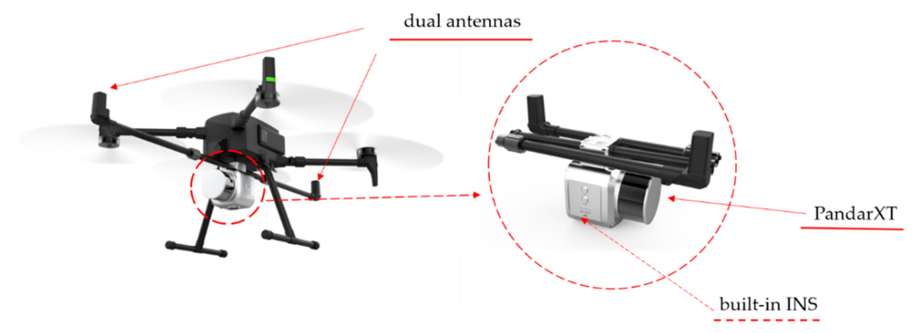
9]. Airborne LiDAR systems (ALS) often integrate with LiDAR sensor units, GPS (Global positioning system) units and INS (inertial navigation system) units, and can be carried on a manned aircraft (e.g., helicopter), a fixed-wing unmanned aerial vehicle (UAV) or a Rotary-wing UAV platform. Manned aircraft LiDAR is restricted by its expensive flying costs and strict airspace application conditions. UAV LiDAR can obtain a wide range of point clouds, and its spatial resolution is relatively high because of its lower flight height and flying speed mode. Rotary-wing UAV LiDAR can closely obtain high-resolution point clouds and have the advantages of flexibility and less strict requirements for take-off and landing, so they become an economical PTL inspection solution and the best choice for small- and medium-sized enterprises and ordinary consumers. Terrestrial LiDAR systems, such as mobile LiDAR scanning systems (MLS), are integrated with LiDAR units, GPS units, Charge Coupled Devices (CCD) units, and DMI units. The MLS often obtains the PTL point clouds only when PTL channels are located in no-fly zones and urban areas. The farther the distance from the scanner, the lower is the obtained MLS point-cloud density, which makes it possible to obtain breakage PTLs [10,11].
For PTLs inspection, the research has mainly concerned power elements detection [9,10,12,13,14,15,16,17,18,19], PTL and pylon reconstruction [20,21,22,23,24,25], safety analysis and simulation [1,7,26,27,28,29]. As the basis of reconstruction and analysis, extraction accuracy of the PTLs determines the effectiveness of reconstruction and recognition of safety hazards. Thus, the PTL classification has received much attention. In recent years, PTL extraction methods have been greatly researched, which mainly include optical images [4,7,30,31,32], thermal images [33] and point clouds [9,15,28,34] acquired from different platforms. Thermal images are used to detect electrical faults but not for 3D reconstruction in high-voltage electric utilities [35]. Because of high resolution and low cost, the optical images are widely applied in PTL extraction. The Hough Transform is a popular method to extract PTLs for images. Nasseri et al. detected PTLs by using the Hough Transform and a particle filter [36]. Song et al. proposed a sequential local-to-global algorithm based on morphological filtering [30]. Fryskowska presented a wavelet-based method for processing data acquired with a low-cost UAV camera [37]. However, the accuracy is unstable and dependent on the quality of obtained images, which are susceptible to natural weather.
Many point-cloud algorithms aiming at power-line extraction have been developed, and most of the extraction methods can be divided into three steps: pre-processing, power-line extraction and refinement. The purpose of pre-processing is to optimize the captured data to reduce interference from non-PTL points and improve efficiency in the subsequent steps. There is a certain distance from PTLs to ground, so the ground points are separated by ground filtering techniques, such as cloth simulation [38] and TIN densification filtering [39], and then the candidate points are selected from non-ground points by height difference filtering [9,12,15,21]. However, ground filtering is a time-consuming process, and pre-treatment results are affected by the terrain in most of these methods. Chen et al. [26]. and Awrangjeb et al. [13] obtained the scope of PTLs by location information about pylons. However, due to various structure types of pylons, complex parameters are required to pick up pylons. Thus, these algorithms are high complexity in their identification of pylons. To eliminate influence of differences in point density from different collection platforms, Zhang et al. [12] and Jung et al. [40] used voxel-based subsampling to balance point cloud density. In addition, data sampling may cause loss of accuracy.
Feature determination and optimization is a critical issue for determining PTL extraction accuracy. Feature-based filters are applied frequently, including eigenvalue features [9,10,12], elevation difference features [13,15] and density features [10,21]. Guan et al. [19] detected PTLs from MLS by combining a height filter, a density filter and a shape filter. Due to low point density and occlusion caused by other objects, the performance of Guan’s method was affected. To solve the accuracy loss caused by uneven distribution or obscured PTLs, Fan used a hierarchical clustering method for extraction in various gap situations [41]. Point-based features are widely applied to extract PTLs by analyzing and calculating points’ properties by neighborhood searching. Certain limitations of differences in corridor terrain and data on distinct platforms could influence the feature stability. Zhang et al. [12] clustered point clouds by dividing voxel data structures, and the PTLs were extracted by eigenvalue and distribution features. The combination of multiple features improves robustness of classification to some extent, which gained our attention. However, there is no in-depth analysis of feature selection and weight in Zhang’s study. There have been some methods that projected point clouds into 2D image structures and efficiently extracted PTLs by existing computer vision processing techniques [42]. Jaehoon et al. [36] used a combination of 2D image features and 3D features to extract power lines and compared various algorithms to prove his method’s superiority in accuracy and efficiency. In the study of Axelsson [43], point clouds were detected from the horizontal XOY plane by using Hough Transform and RANSAC algorithms. Munir et al. combined 2D grid and 3D point-based structures to extract individual conductors [44]. However, the 2D projected methods cannot deal with the interference points in the vertical direction, and the data conversion between 2D images and 3D points may cause the loss of extraction accuracy. Meanwhile, the existing algorithms have no in-depth study concerning how to select features and quantify the importance of different features to optimal extraction.
Furthermore, machine learning is another strategy for PTL extraction. The popular supervised classifiers include JointBoost [45], support vector machine (SVM) [16,46], random forest (RF) [6,37,47] and adaptive boosting (AdaBoost) [16]. Precision is closely related to selection of classifiers. Guo et al. [45] used the JointBoost classifier and a graph-cut segmentation algorithm to classify PTLs. Suresh K. Lodha et al. compared the SVM classifier with the AdaBoost classifier and concluded that the extraction performances of SVM and AdaBoost are similar [14]. Wang et al. [46] compared six classifiers and found the random forest was the most suitable for extracting PTLs, and Peng et al. [8] reached the same conclusion. By executing SVM classifier training, Wang et al. proposed a multi-scale slant cylindrical neighborhood-searching algorithm for spatial structural features extraction, and then extracted PTLs by multi-scale features [46]. Yang et al. classified PTLs using a random forest that was optimized by Markov Random Field [48]. Machine learning methods can obtain excellent extraction accuracy, but the unbalanced samples and data gaps could affect the success rate of extraction. Meanwhile, the time-consuming nature of samples training makes it expensive for PTL classification. It is limited by the differences (point densities, various terrains) in data across different platforms. With the continuous improvement of computer performance and excellent performance of deep learning technology in target recognition, researchers have become interested in using deep learning to classify transmission line scenarios. At present, there are two commonly used deep learning strategies for power scenarios. In the first strategy, 2D feature images converted from 3D point clouds are applied to 2D CNNs for classification [49]. However, transforming unstructured 3D point sets into regular representation inevitably may cause spatial information loss. The second one is to use PointNet [50], PointNet++ [51], PointCNN [52] and so on to classify transmission line scenarios. These models are overly dependent on sample training and cannot obtain stable classification accuracy with different data.
A post-processing refinement step is employed to improve the accuracy of PTL extraction. Jaehoon et al. [36] rasterized candidate power-line points onto 2D binary images, removing error points using image-based filtering. Zhang et al. [12] and Awrangjeb [13] analyzed the positional relationship between pylons and PTLs in the 3D space to filter out false positives. In addition, PTLs also can be refined by modelling. The PTLs can be fitted using 3D mathematical models, which consist of two parts: a XOY projection plane model and a vertical projection plane (XOZ plane or YOZ plane) model [21]. Alternatively, a catenary curve model also can be applied to reconstruct the PTLs [22]. Post-treatment may cause a few of the power-line points to be missing and increase time consumption as well.
Overall, there is a lot of advanced work on PTL extraction. However, there are still limitations on generality and efficiency. For the most unsupervised methods, extraction accuracy overly depends on the performance of the pre-processing step. Prior information, such as vehicle trajectory and sample data, as well as classified pylon point clouds or pylon coordinates are required, which affects the generality of many algorithms. Some algorithms depend heavily on the stability of features. In complex environments (e.g., mountains, cities), accuracy reduction of extraction results from the proximity of PTLs to vegetation or buildings. The popular algorithms extract PTLs by hierarchical-multiple-rule evaluation of many geometric features, which need strict input parameters. When extracting PTLs from different scenes, manual intervention is necessary to achieve stable extraction results. To achieve efficient PTL extraction for different platforms and complex scenes, this paper proposes a method based on entropy-weighting feature evaluation (EWFE), which focuses on efficient PTL extraction by using as few salient geometric features as possible and achieving robust extraction with few parameter adjustments.
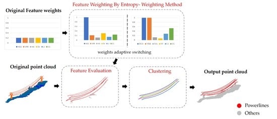
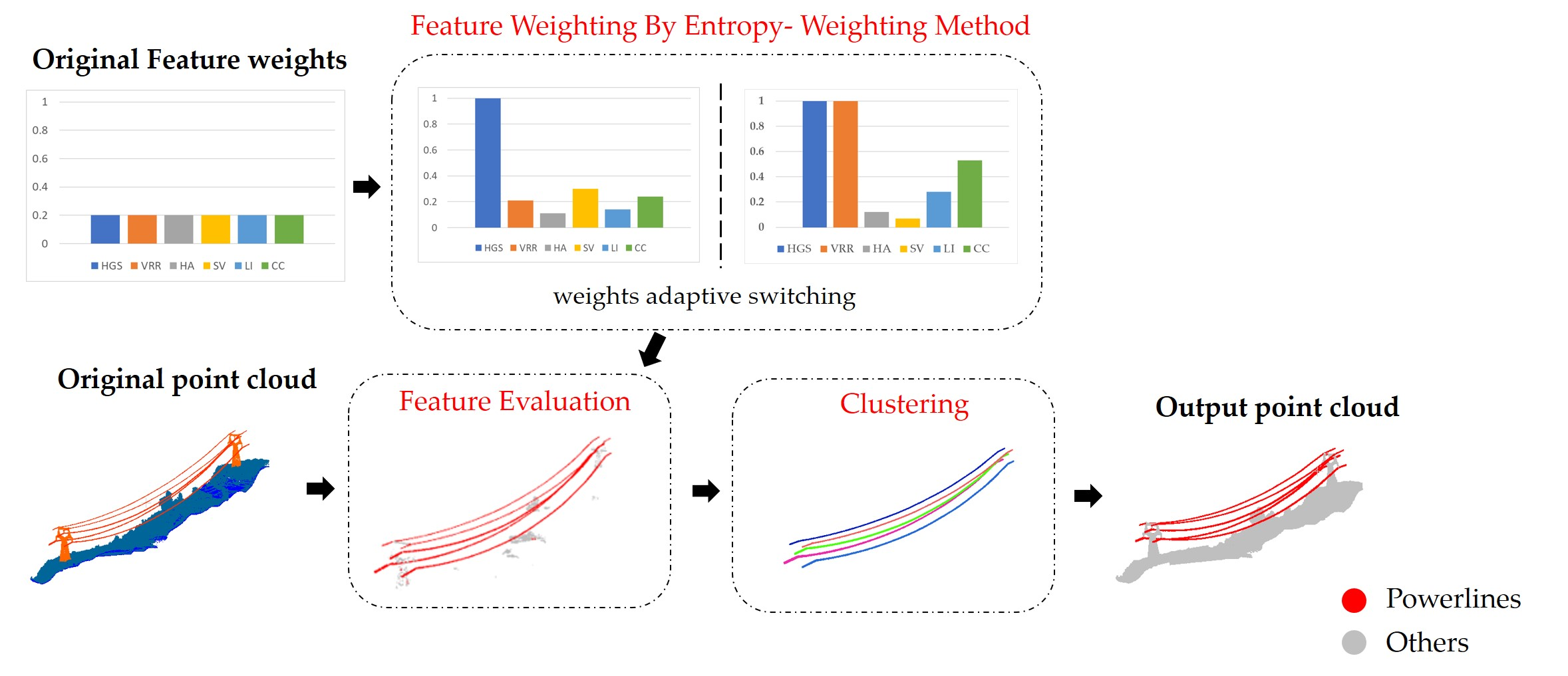
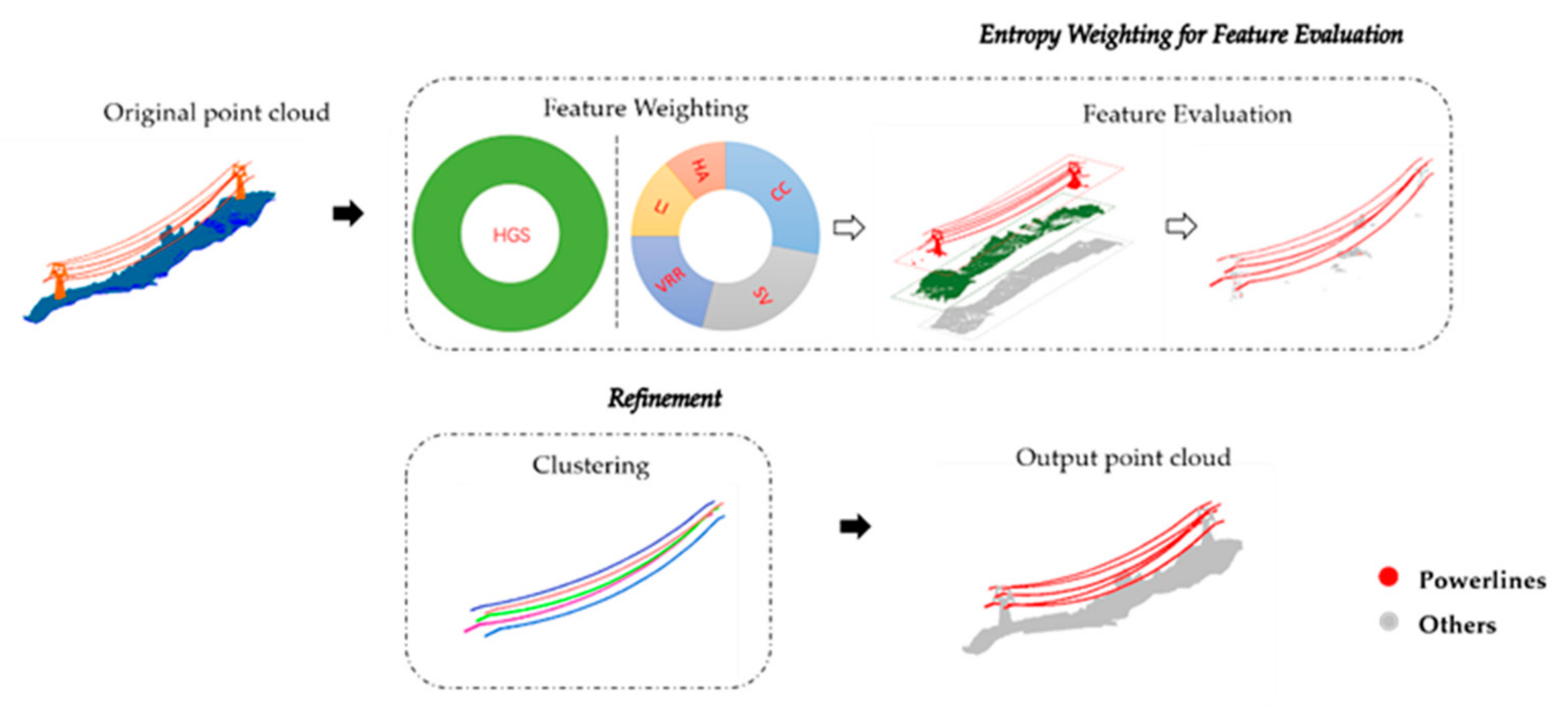
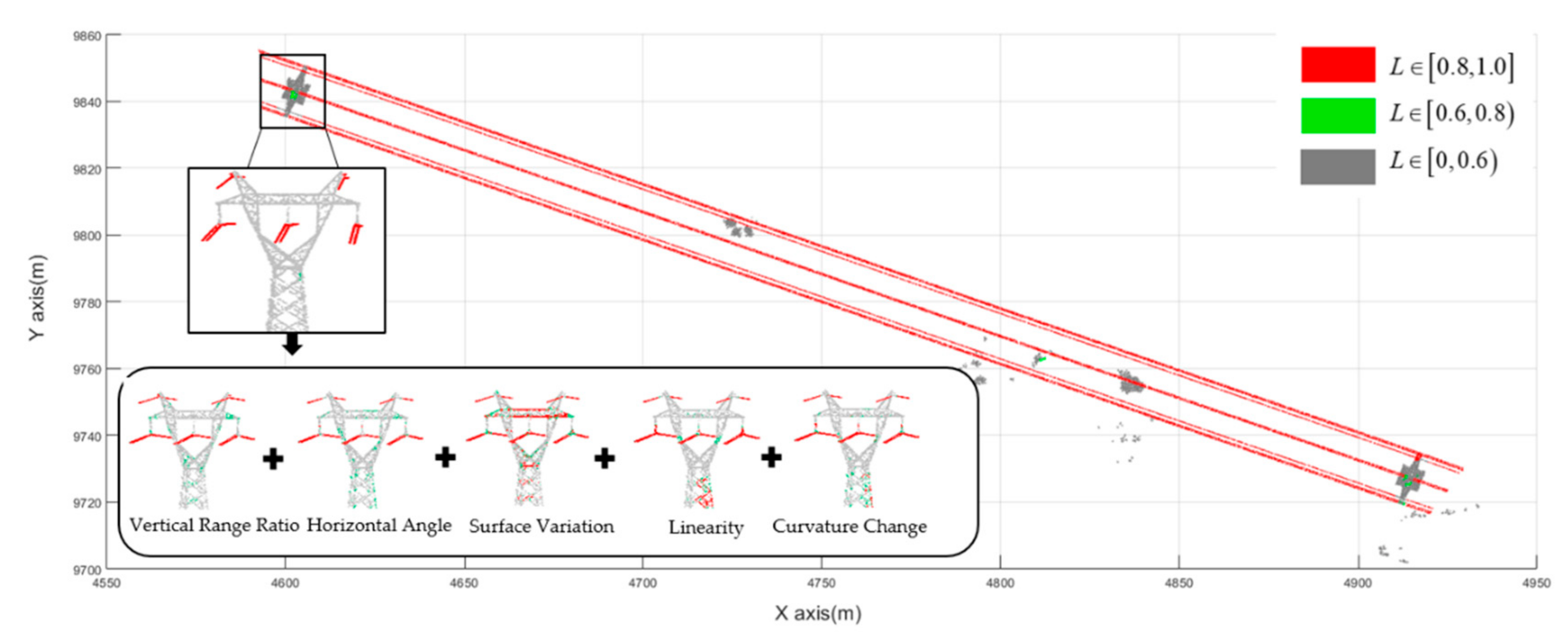
A feature vector is constituted by analyzing six salient features (SSFs) including Height above Ground Surface (HGS), Vertical Range Ratio (VRR), Horizontal Angle (HA), Surface Variation (SV), Linearity (LI) and Curvature Change (CC). After the feature information normalization, the weights of the SSFs are calculated and assigned by entropy-weighting method. The point clouds are filtered by the HGS feature, which can improve the processing efficiency by removing most non-PTL points with minimal PTL loss. Then, PTLs are extracted by the remaining five features evaluated by an adaptive feature-weighting algorithm. Noises are finally removed by clustering. The whole workflow of the proposed EWFE algorithm is illustrated in Figure 1.
This paper is structured as follows: Section 2 describes the datasets and analyzes the proposed method in detail. Experiments are provided for describing the applicability of the proposed detecting method in Section 3. Discussions about the influence of feature weighting distribution and real-time detection analysis are presented in Section 4. Finally, Section 5 concludes this work and provides plans for the future.

2. Materials and Methods

2.1. Datasets

To test effectiveness of the proposed EWFE PTL extraction method, we obtained four datasets from different platforms. The first three datasets were collected by CBI-200P, a light and small LiDAR system weighting about 1.6 kg. The CBI-200P system was carried on a quad-rotor UAV platform. It integrates a PandarXT laser scanner and a built-in Inertial Navigation Unit (INS), and two identical antennas are located at each end as illustrated in Figure 2. The ranging accuracy of PandarXT is 2 cm, its effective range is about 200 m and the vertical angular step width is set to 0.2°. These three datasets are each located in different PTL corridor scenes, and they are named Sanmenxia 220 kV (Dataset 1), Mianyang 500 kV (Dataset 2) and Chongqing 220 kV (Dataset 3) by the place names and voltage level for convenience of memory. To test the performance on different platforms, the last dataset was obtained from urban street scenes in Wuhan by a vehicle-borne LiDAR system, where the transmission voltage level is 110 kV. The vehicle-borne LiDAR system integrates a Rigel-VUX scanner and was carried on a vehicle for accurate data acquisition. The ranging accuracy of the Rigel-VUX is 5 mm, and the vertical scan angular step width is selectable and was set to 0.015°. Laser beams from a laser scanner are reflected off the targets and back to the receiver to obtain target point-cloud data. Point-cloud data contain three-dimensional coordinate information of spatial objects, as well as the intensity, echo number and other information.
Geographic information about the four datasets is revealed in Figure 3, where detailed terrain is exhibited at the corridor example site. Dataset 1 was colllected from a rural area that contains large amounts of farmland, including mountain terrain with significant elevation fluctuation in the first half of data and flat terrain with farmland and low vegetation in the second half of data. Dataset 2 was scanned from a flatland with little vegetation and about 0.95 km length. Dataset 3 was collected from a complex scene including mountain terrain. Dataset 4 includes two corridors, lies in an urban area, and was collected by mobile LiDAR. Due to the limitation of distance or occlusion, there are some PTLs missing and broken in Dataset 4. The flying or driving speed during all data collection was from about 5 m/s to 8 m/s. The detailed information on the four datasets is summarized in Table 1.

2.2. Features and Significance

The construction and calculation of features determine the precision and result of PTL classification. The power lines are distributed between two neighboring electric pylons or poles with sag and are regular and linear. Furthermore, there are obvious differences between power lines and other ground features in physical size and spatial distribution. Thus, we constructed the point-cloud features by analyzing the spatial distribution characteristics and surface characteristics of the PTLs. We chose different local neighborhoods to obtain each point with a series of fixed parameters, which includes the search radius, k-nearest neighborhood and so on. The features are used in the classification of the power lines and other objects.
The designed features mainly fall into the following three categories: Height features, Eigenvalue features and Density features, as listed in Table 2. The transmission line scene includes many different ground objects, such as ground, vegetation, buildings, towers and PTLs. Certain features make it difficult to distinguish power lines from other objects, resulting in relatively less contribution of these features to classification accuracy. The features that are similar to target ground object characteristics or can suppress non-target objects should be selected. After testing one by one, we selected the SSFs, including height features (HGS and VRR) and eigenvalue features (HA, SV, LI and CC), as the features of the proposed EWFE algorithm to distinguish PTLs from other ground objects.
Height features: The PTLs are suspended on utility pylons and located in clearance regions at a certain distance to ground surface. There are industry criterions for different transmission voltage scales in China [53] or America [19]. By establishing 2D grid structures on the XOY projected planes, the minimum height of point in all grids was regarded as the reference ground height. The Z ground is the minimum Z coordinate in grids, as shown in Equation (1) The HGS feature H G can be used to judge the approximate spatial relationship between the object and the ground.
Z ground = min { Z i }
3D voxel structures were established as point-cloud storage units. The VRR represents the ratio between the max–min height difference and the length of a voxel. A voxel is considered as the processing unit, and all points have the same VRR feature. According to the coordinates, the voxels were built and the points were distributed into each voxel according to Equation (2). Figure 4 shows the different object point clouds with voxels. Different ground objects have different VRR feature values in the voxel. The objects with vertical structure can be identified by VVR.
R = x i x min / l ; C = ( y i y min ) / d ; L = ( z i z min ) / h ;
In this equation, ( R , C , L ) represent the row, column and layer index of the voxel for i -th point. ( l , d , h ) represent the length, width and height of all voxels.
Eigenvalue features: The power lines are linear and continuous. Eigenvalue features can distinctly extract linearity, edge and plane, which are used to distinguish PTLs and other objects (e.g., vegetation) popularly [12,15]. Point clouds were stored in a kd-tree, and then eigenvalues and eigenvector were computed by the points searched in k-nearest neighborhood. The HA ( H A ), SV ( S V ), LI ( L I ) and CC ( C U ) features were calculated from eigenvalues and eigenvectors.
To analyze the performance of SSFs on different types of objects, feature values were computed and assigned to three intervals: high, medium and low. As is illustrated in Figure 5, we tested the SSFs in a transmission line scene and obtained the performance distinction between PTLs and other objects. The HGS, SV and LI features were referred to as positive features in which PTLs are in a high characteristic interval. Inversely, the VRR, HA and CC were called negative features. HGS can distinguish ground, low vegetation and building. VRR and HA can filter a portion of towers and vegetation, and HA has better performance in distinguishing vegetation. SV and LI can detect power lines with few noises. Different features can distinguish different objects. The combined evaluation of features can improve the robustness of the model.

2.3. Feature Weights Determined by Entropy-Weighting Method

The existing hierarchical-multiple-rule extraction methods [9,12,18,21,30,34] are generally adopted to classify PTL points, for which construction and calculation of multiple features through threshold rules step by step determined the final detection accuracy. These approaches created a high requirement for stability of the constructed features. Due to the diversity of data quality and power transmission scenes, it is difficult for all PTLs to obtain a stable performance in each feature. Thus, the extraction accuracy could be affected. To improve the robustness of classification, we extract PTLs by comprehensive feature evaluation. Whether points belong to power lines is determined by the evaluation of all features, which can reduce the effect of feature instability on accuracy. As mentioned in Section 2.2, different features have different contributions for PTL extraction. We should give the features which possess the stronger detection ability and robustness greater weight in the evaluation process.
To determine the optimal feature weights to maximize the performance of the feature combination, this paper uses the entropy-weighting method (EWM), by which different weights are given to different performance features. Entropy was originally a concept in thermodynamics and was introduced to information theory by C. E. Shannon [54]. The EWM, as a comprehensive evaluation method that is applied to describe indexes in a complex system, has been widely used in many popular fields (e.g., engineering and economics). In information theory, entropy represents the degree of chaos in a system [55]. It can also quantify the amount of information provided by each index and analyze the proportion of each indicator in the system. The quantity of information is quantified as the concept of entropy value and entropy weight [56]. The basic ideas of the EWM are as follows: The entropy values of indicators are in inverse proportion to their entropy weighting. In a certain index, if the data of one object vary considerably, according to information theory, its entropy would be low. That means that if the object could contribute much useful information, its entropy weight would be high. Otherwise, the entropy weight should be low correspondingly. The determination of entropy weights requires the information provided by the samples. The selection of samples can affect the final entropy weights. We found that there are significant weight changes in two typical scenes where the power lines hang from pylons and away from the pylons. Two samples from the Sanmenxia 220 kV data (Dataset 1), including the sample near the pylons and the sample away from the pylons, were used to calculate the entropy weights. There are three steps to obtain the weight distribution by EWM.
(1) Feature information matrix construction and standardization. A feature information matrix reflects the information of each feature. Each element in the matrix is an evaluation of each point according to the SSFs. To eliminate the influence of unit magnitude and scale on the feature matrix, the feature values are normalized from 0–1 by min–max threshold intervals. The HA, SV and LI are positive features by which the PTLs are distributed in a high characteristic range. Thus, the higher the feature values, the more likely a point is to be a PTL and the better its evaluation. On the contrary, the VRR, HA and CC are negative features. The lower the feature values, the better the evaluation. The traditional entropy-weighting method evaluation indicators are limited to error and data accuracy, making it hard to obtain maximum or minimum feature values in relation to PTL extraction. Thus, we optimized the evaluation by setting the threshold interval instead of the extreme value to improve robustness, and the detailed calculation equation is Equation (3):
positive   feature V i j > V high , e i j = 1 V i j ( V l o w , . V high ) , e i j = V i j V l o w ( V high V l o w ) V i j < V l o w , e i j = 0 , ( i = 1 , , 6 ; j = 1 , n ) negative   feature V i j > V high , e i j = 0 V i j ( V l o w , . V high ) , e i j = V high V i j ( V high V l o w ) V i j < V l o w , e i j = 1 , ( i = 1 , , 6 ; j = 1 , n )
where ( V l o w , . V high ) separately represent the minimum and maximum thresholds; e i j represents the evaluation value of the i-th feature on the j-th point.
The comprehensive evaluation information matrix is shown in Equation (4).
E = ( e i j ) 6 × n = e 11 e 12 e 1 n e 21 e 22 e 2 n e 61 e 62 e 6 n , ( i = 1 , 2 , 6 ; j = 1 , 2 , n )
(2) Entropy-weighting calculation. The entropy value is determined by the degree of stability, either high and low, of each point evaluation value of a feature. The entropy value of the i-th feature is calculated by Equation (5) by referencing Zhao’s research [57]:
S i = 1 ln n j = 1 n P i j ln P i j ; P i j = e i j j = 1 n e i j ( i = 1 , 2 , , 6 ; j = 1 , 2 , , n )
where P i j represents the index proportion of the i-th feature on the j-th point, and S i represents the entropy value of the i-th indicator. When P i j = 0 , P i j ln P i j = 0 .
After computing the entropy value of each feature, the entropy weight is calculated as in Equation (6):
ω i = 1 S i i = 1 n ( 1 S i ) = 1 S i n i = 1 n S i , ( i = 1 , 2 , 6 )
where ω i represents the entropy weight of i-th feature, 0 ω i 1 , i = 1 6 ω i = 1 .
(3) Feature-weighting calculation. The entropy weights are in inverse proportion to the final feature weights of feature-based classification. If a feature displays a smaller entropy value than the other features, it means that the point clouds possess a stronger order and lower uncertainty for this feature. In other words, this feature is more conducive to information extraction and possesses a higher weight value. The inverse relation between the final weight ω i and entropy weight is shown in Equation (7).
ω i = ( 1 / ω j ) i = 1 6 ( 1 / ω i ) , ( i = 1 , 2 , , 6 )
After analyzing the entropy weights, we obtained the final weights in two sample scenes. As shown in Table 3, the entropy of the HGS feature is computed as 1 in both samples, which means the HGS feature can keep the all PTL information and remove a portion of the other object points. Thus, the HGS feature can achieve separate evaluation without PTL precision loss. When away from the pylons, the SV has the highest weight (0.3) among the remaining features, which indicates that it has the largest contribution to power-line extraction in this scene. In the area close to pylons, the weight of the VVR feature is 1, which is the same as the HGS feature. Among the remaining features, the CC has the highest weight (0.53).

2.4. Feature Evaluation

The PTL points are extracted by feature evaluation. Because the entropy value of HGS feature is 1, the LiDAR points are separately evaluated by the HGS feature to remove a portion of the non-PTL points. The remaining points participate in subsequent evaluation. The advantage of this step is that it can improve the efficiency of subsequent feature calculation and directly eliminate the interference of non-PTL points in power-line extraction. Then, the original evaluation information matrix is formed. Through the evaluation information matrix and the weight matrix, the PTL points are extracted by the comprehensive feature evaluation. The HGS feature evaluation c and the comprehensive feature evaluation E are calculated by Equation (8):
C = e j ω HGS , ( j = 1 , 2 , , n ) C = E ω = e 21 e 22 e 2 n e 31 e 32 e 3 n e 61 e 62 e 6 n ω VVR       ω HA       ω SV       ω LI       ω CC
where n represents the number of points and n represents the number of points which are selected by HGS evaluation.
The weights are different between the pylon area and the area away from pylons. These two types of areas constitute the complete power-line point-cloud data. To realize the weights’ adaptive switching, we designed a moving window to detect the pylon areas. Pylons have distinct geometric characteristics. In the vertical direction, there is a certain gap between power lines, while each pylon has strong vertical continuity and HGS feature. The pylon regions can be judged by these two characteristics. The process of pylons detection is shown in Figure 6.
The feature evaluation results are shown in Figure 7 Most of the PTL points were extracted out, but there were a few erroneous extractions of points from pylons and vegetation objects when the evaluation threshold E was set at 0.6–0.8. If E rose to 0.8, the number of erroneous extraction points was greatly decreased.
The extraction results of two different types of towers before and after adaptive weights transformation are shown in Figure 8. The adaptive weights can effectively reduce the phenomenon of error extraction in the pylons without manual intervention. After feature evaluation, the extracted points may still include a few noisy non-PTL points with similar linearity. The noises are irregularly distributed in pylons and buildings generally. To remove the noises, the point clouds were grouped into a set of clusters by Euclidean distance clustering. The points in the clusters whose lengths were less than a predefined length threshold ( l min ) were considered noises.

3. Experiments and Analysis

3.1. Evaluation Metrics

For most of the past methods, precision, recall and F1-score were recommended for evaluating the PTL extraction performance of the EWFE algorithm, as in Equation (9). The extracted point clouds were compared with the reference datasets, which were labelled manually by using Alundar point-cloud-processing software downloaded from the website (www.a-lidar.com) in 1 June 2021. The efficiency of the method was evaluated by calculating the ratio of running time (sec) to points number (millions), where the running time of data reading and writing was not counted. The proposed method was programmed on Microsoft Visual Studio 2015 with C++ 11 standard. The datasets were tested on a common laptop with i7-9750H and 16G RAM.
Precision = TP TP + FP , Recall = TP TP + FN , F = 2 / ( 1 Precision + 1 Recall )
In this equation, TP is the number of correctly classified PTL points, FP represents the number of non-PTL points that are incorrectly detected as PTL points and FN represents the number of PTL point that are labelled as non-PTL points.

3.2. Parameters Sensitivity Analysis

The algorithm parameters were separately tested to obtain the optimal setting and were set by standard, empiric and significance analysis. The standard parameters were adaptively changed according to different transmission line scales. After significance analysis, the radius for neighbor search is recommended to be set to 3 m. Compared with the rule-based thresholds, the threshold intervals that were confirmed by the feature significance comparison are more robust, because they provided buffer zones. In different datasets, the PTL points may be not in the optimal threshold for every feature interval, but the most of the PTL points can be within an excellent threshold range for the feature intervals of the feature vector. Thus, the threshold intervals possessed low sensitivity. The E HGS can be automatically set according to the clearance distance standards of different transmission scales and can also be modified manually to improve the efficiency of the algorithm. We tested the four threshold interval parameters ( H min , H max , S min , S max , C min , C max , L min , L max ) and there were four threshold intervals for each parameter. The tests also proved that the threshold intervals had steady performance. The empiric parameters may need to be set experimentally based on the case’s requirements to achieve the best performance. After the parameter tests, we listed all parameters and suggested values of the proposed approach in Table 4.
To obtain the specific effects on extraction accuracy of empiric parameters changing, we tested the empiric parameters (evaluation threshold E t and minimum length of line l min ) to understand how much they affect accuracy. Five fragments, which are site A-1 in Dataset 1, site B-1 in Dataset 2, site C-1 and C-2 in Dataset 3 and site D-1 in Dataset 4, respectively, were chosen as test data. The evaluation standard chosen was an average F1-score to evaluate parameter sensitivity. The results are seen in Figure 9. The average F1-score is in an excellent and stable range (99.2–99.04%) for the minimum length of line l min . The highest F value is just about greater 0.16% than the lowest F1-score on l min . Conversely, the influence of the evaluation threshold E t on accuracy is more obvious. The F1-score ranges from 99.2% to 95.4%, and the highest F value differs by 3.8% from the lowest F value of l min . The minimum length of line has lower sensitivity than the evaluation threshold. The changing of l min has a small influence on precision, which is acceptable. The evaluation threshold determines the result of feature evaluation and may change for different datasets to obtain the optimal extraction accuracy.

3.3. Results and Analysis

The extracted PTL results are shown in Figure 10 by using the suggested algorithm parameters. For the four datasets, only empiric parameters were manually adjusted, and other parameters were kept consistent or adapted to change, as seen in Table 4. The extracted PTLs are labelled with red color in Figure 10. The zoomed regions show the detailed extraction results. The PTLs were detected accurately from all four datasets. Even in steep mountains (Dataset 1 and Dataset 3) and urban areas with sparse PTL density (Dataset 4), the PTLs could also be precisely separated from ground, vegetation and building objects. The EWFE algorithm could maintain stable extraction results for single 110 kV PTLs (Dataset 4), twin-bundled 220 kV PTLs (Dataset 1) and quad-bundled 500 kV PTLs (Dataset 2 and Dataset 3). This shows the proposed method can provide a stable evaluation to differentiate PTLs and non-PTLs, thus producing accurate and efficient PTL detection results.
The recall, precision and F1-score of all datasets are listed in Table 5. The recall and precision were distributed between 98.8% and 99.9% and between 97.6% and 99.9%, respectively. The efficiency was calculated to be between 1.2 and 5.9 million points per second. Benefitting from the flat terrain, the F precision of Dataset 2 was the highest at about 99.7%. The poor result with Dataset 4 is due to low-density PTL points (2.1–18.9 points/m3) being inaccurately removed. Furthermore, there are some fracture PTL points that were filtered as noises during the clustering step. Benefitting from the excellent performance of feature evaluation, there were no vegetation, ground or building points extracted as PTLs in the four datasets. The HGS feature evaluation determines the number of subsequent points involved in the calculation of complex features. Thus, the evaluation threshold parameter is an important factor that affects the efficiency of the algorithm. Due to the steep terrain, we set a more relaxed evaluation threshold to ensure that there was no loss of power-line accuracy in Dataset 1. Thus, the efficiency of Dataset 3 was the lowest (0.9 million points/s). The highest efficiency was from Dataset 4 (5.9 million points/s). In urban areas, the terrain is flat, and more non-PTL objects can be filtered by HGS feature evaluation.
Two typical false-extraction scenarios are shown in Figure 11. Because the drainage lines are related to the power lines and have linear structure, it is easy to misidentify them as PTLs, resulting in a loss of precision. Figure 11a shows the drainage line that was extraction as a PTL in Dataset 1. Due to occlusion, partly by other PTLs, there are partially fractured power lines in Dataset 4. The EWFE can still accurately identify the power lines at both ends of the fracture. However, there are a few sparse point clouds that are not correctly identified (Figure 11b). By analyzing the fragment PTLs, we found the sparse PTLs can be excellently identified by feature evaluation. Unfortunately, these PTLs are easily filtered during the refinement step. After reducing the minimum length of line ( l min ), more discrete PTLs can be retained with more noises.
To evaluate the efficiency of each step in the EWFE algorithm, this paper lists the point numbers that were calculated in each step in Table 6 and the time consumption of each process in Table 7. According to the entropy-weighting feature evaluation, the HGS feature evaluation eliminated the most points and provided a high efficiency process with cost-effective time consumption. For example, the HGS feature can filter 98% of the non-PTLs in 3.7% of the whole process’s time consumption. Due to its complex domain search and computation, eigenvalue features calculation took the largest proportion of time consumption, including 65.8% for features calculations in Dataset 1, 77.5% in Dataset 2, 85.7% in Dataset 3 and 64.7% for Dataset 4. Fortunately, the high-time-consumption feature evaluation brings higher accuracy benefits, even in the absence of clustering. The clustering only removed a small number of points, which proved only a small amount of noises were extracted.

3.4. Comparative Study

We tried to utilize Zhang’s method [10] and Jaehoon’s method [38]. After the parameter optimization, we tried to reach the best classification performance of these methods in the four datasets. The results are listed in Table 8. Zhang’s method was proposed for UAV LiDAR, so it was not tested in Dataset 4. All three methods had the highest precision performance in Dataset 2, for which the terrain is flat and the vegetation is far away from the PTLs. In Dataset 3, the complex terrain variation affected the algorithm performance. Compared with the performance on Dataset 2, the F fell 1.1% for our method, 1.4% for Zhang’s method and 1.8% for Jaehoon’s method. In Dataset 4, the broken PTLs posed a challenge to Jaehoon’s method. There were a few broken PTLs which the method failed to extract. Thus, the precision and F of Dataset 4 were the lowest. Compared with Zhang’s method, Jaehoon’s method acquired more outstanding performance in terms of precision. In Jaehoon’s method, the refinement step, which includes a series of optimization processes, is an important factor in removing noises. Benefitting from the excellent performance of adaptive feature evaluation, the precision of our method for the four datasets was obviously better than Zhang’s method and Jaehoon’s method.
The efficiency in Table 9 is calculated by dividing the number of all dataset points by the time consumption listed. For contrast, the efficiency presented in the literature was recorded in the parentheses. It should be noted that the time consumption does not account for loading and writing the data. Unfortunately, Zhang’s method did not measure the separate PTL extraction time. The time consumption includes the time of tower extraction and PTL extraction. Thus, the efficiency of Zhang’s method must be greater than 1.1. Due to the ground filtering and a series of elaboration steps, the efficiency of Jaehoon’s method was the lowest (1.2 million points/s). In the EWFE and Zhang’s method, feature calculation is the most time-consuming step, which is unavoidable. In the EWFE method, HGS evaluation filtered out most of the non-PTLs. The EWEF simplifies the pre-processing and the post-processing steps. Thus, the efficiency of the EWFE is higher than that of Zhang’s and Jaehoon’s methods. The proposed method could be more efficient if parallel computing is used.

4. Discussion

4.1. Influence of Feature Weighting on PTL Extraction

Different features have different levels of contribution. Feature weighting is an extremely important factor in the accuracy of extraction. For the quantitative assessment of the EWFE algorithm, two different weighting strategies are employed: average weight feature evaluation (AWFE) and the EWFE method. AWFE gives equal weighting values to all feature items. Furthermore, the rule-based extraction was implemented and compared, which is a popular strategy in others’ research [12,21]. The algorithm parameters of the three strategies were set by sensitivity experiments to obtain optimum effect separately. The points were judged to be PTLs only when their performance was qualified in each feature in rule-based extraction. If any feature performance did not meet the threshold requirement, points were determined as non-PTLs. These three methods were selected from SSFs. The precision results are illustrated in Figure 12. The rule-based extraction had poor performance in precision, recall and F in the four datasets. Dataset 4 in particular had obvious PTLs missing, with its accuracy apparently further reduced than in the other datasets. Compared with rule-based extraction, the accuracy of the AWFE strategy showed a significant improvement. Of the three strategies, the accuracy of the EWFE strategy was the highest in all datasets. The F of the EWFE strategy separately increased 3.3%, 0.8%, 3.5% and 1.6% compared to the AWFE strategy. The results indicate that feature evaluation can improve PTL extraction effectively. On the basic of this, entropy-weighting allocation for features can further optimize precision.

4.2. Real-Time PTLs Extraction by EWFE

UAVs are becoming the most widely used power-line inspection platforms because of their convenience, low cost and short-distance collection with high-resolution data. LiDAR point clouds are scanned by UAVs, and this process depends on advance flight-path planning. Inaccurate flight paths may result in poor quality of the captured point clouds, or even UAVs crashing. However, during the flight, UAVs usually cannot reliably perceive whether their flight paths are correct and safe or not. Real-time detection could help UAVs by giving them PTL geometric position information to assist path planning and improve obstacle avoidance abilities. Thus, there has been increasing interest in the application of real-time PTL detection.
At present, there is little research on real-time power-line extraction. However, there are similar studies on wildfire detection [28] and 3D object detection [58,59]. Due to distance and real-time limits, distal PTLs are sparse and hard to extract, which poses a challenge to the robustness of an extraction algorithm. With the popularity of UAV LiDAR systems, the point-cloud density is greatly increased compared with manned aircraft LiDAR systems. The input data are raw high-density point clouds. Thus, real-time detection requires high efficiency. To analyze the effect of real-time extraction on the EWFE algorithm, we tested the three datasets captured by UAV LiDAR. The scanning frequency of the laser scanner was 20 Hz (20 frames per s), and the fly speed was maintained at 5 m/s. We segmented the raw point clouds by 2 s. Thus, the UAV flew about 10 m and the laser scanner completed 40 frames within 2 s. Compared with the raw point clouds, the time intervals data had a significant decrease in the average point density (415 pts/m2 to 42 pts/m2). The point density of different time intervals can be different. At the edge of the data, the PTL density dropped to a fairly low range (within 5 pts/m2). We used the same implementation environment and laptop with the experiments in Section 3.3. After extracting, we combined five copies (total 10 s, 200 frames) of data as a block to display the intuitive extraction effect and calculate efficiency. Figure 13 shows a portion of blocks which came from Dataset 3. The same effect can be observed in other blocks and datasets.
The EWFE algorithm turned out to be efficient, and accurately detected PTL points with the density changing. The majority of sparse PTL points at the far end were also identified. In all blocks, there are no obvious errors in extraction or missing extractions. In terms of efficiency, the time consumption of classification was kept within a satisfactory range. The average reading and running time of 20 frames of data was 0.013 s. The PTL extraction running time of 20 frames ranged from about 0.019 s to 0.126 s. Even in the block with dense towers among the point clouds, the total time consumption, which includes reading consumption and classification consumption, was only 0.139 s/20 frames. The efficiency of the algorithm can meet the demand of real-time PTL classification.

5. Conclusions

This paper proposes an accurate PTL extraction method by using entropy-weighting feature evaluation (EWFE) for UAVs and mobile LiDAR point clouds. To achieve efficient extraction, a feature vector constituted by six geometric features including Height above Ground Surface (HGS), Vertical Range Ratio (VRR), Horizontal Angle (HA), Surface Variation (SV), Linearity (LI) and Curvature Change (CC) is used. The feature values are normalized to eliminate the influence of unit magnitude and scale among the features. The characteristic weights are calculated by the entropy-weighting method. The first feature is evaluated to filter out a portion of non-PTLs. Then, PTLs are extracted by the other five features’ evaluation. The EWFE algorithm is applicable to mobile LiDAR and UAV point clouds without any supplemental data, and thereby improves the utility. It can extract PTLs accurately without pre-treatment, such as ground filtering, which improved the efficiency. When tested in four different datasets after sensitivity analysis, the average F precision is about 99.1%, and the average efficiency is 2.5 million points/s.
In the discussion, we chose another two different extraction strategies to compare with the proposed EWFE algorithm to confirm that the EWFE algorithm can improve the extraction accuracy to a certain extent. Furthermore, we discussed the potential use for real-time classification of the EWFE algorithm. In terms of efficiency, EWFE can meet the efficiency requirements of real-time extraction with excellent extraction accuracy. Nevertheless, the proposed method has the following issues, which need to be further investigated. There were a few towers and insulator points detected as PTLs mistakenly. How to optimize the extraction of pylon connections without precision loss is the focus for future work. Multi-scale features have attracted our attention for this question. In addition, after detecting PTLs, refined tower and insulator extraction is also of interest for our future study.

Author Contributions

Conceptualization, J.T. and H.Z.; Data curation, R.Y., H.L. and S.L.; Funding acquisition, J.T.; Methodology, J.T. and H.Z.; Resources, S.L.; Software, H.L. and J.L.; Supervision, S.L. and J.L.; Validation, R.Y., H.L. and S.L.; Visualization, J.T., H.Z. and R.Y.; Writing—Original draft, J.T. and H.Z.; Writing—review and editing, J.T., H.Z., R.Y., H.L., S.L. and J.L. All authors have read and agreed to the published version of the manuscript.

Funding

This research was funded by the Science and Technology Plan Project of Sichuan Province (Grant number 2021YJ0369).

Acknowledgments

We would like to thank Chengdu Alundar Technology, China, and Wuhan Rgspace Technology, China, for providing the experimental data and to thank the anonymous reviewers for their valuable feedback.

Conflicts of Interest

The authors declare no conflict of interest.

References

  1. Xu, K.; Zhang, X.; Chen, Z.; Wu, W.; Li, T. Risk assessment for wildfire occurrence in high-voltage power line corridors by using remote-sensing techniques: A case study in Hubei Province, China. Int. J. Remote Sens. 2016, 37, 4818–4837. [Google Scholar] [CrossRef] [Green Version]
  2. Matikainen, L.; Lehtomäki, M.; Ahokas, E.; Hyyppä, J.; Karjalainen, M.; Jaakkola, A.; Kukko, A.; Heinonen, T. Remote sensing methods for power line corridor surveys. ISPRS J. Photogramm. Remote Sens. 2016, 119, 10–31. [Google Scholar] [CrossRef] [Green Version]
  3. Yan, G.; Li, C.; Zhou, G.; Zhang, W.; Li, X. Automatic Extraction of Power Lines from Aerial Images. IEEE Geosci. Remote Sens. Lett. 2007, 4, 387–391. [Google Scholar] [CrossRef]
  4. Oh, J.; Lee, C. 3D Power Line Extraction from Multiple Aerial Images. Sensors 2017, 17, 2244. [Google Scholar] [CrossRef] [Green Version]
  5. Siranec, M.; Höger, M.; Otcenasova, A. Advanced Power Line Diagnostics Using Point Cloud Data—Possible Applications and Limits. Remote Sens. 2021, 13, 1880. [Google Scholar] [CrossRef]
  6. Watts, A.C.; Ambrosia, V.G.; Hinkley, E.A. Unmanned Aircraft Systems in Remote Sensing and Scientific Research: Classification and Considerations of Use. Remote Sens. 2012, 4, 1671–1692. [Google Scholar] [CrossRef] [Green Version]
  7. Zhang, Y.; Yuan, X.; Li, W.; Chen, S. Automatic Power Line Inspection Using UAV Images. Remote Sens. 2017, 9, 824. [Google Scholar] [CrossRef] [Green Version]
  8. Peng, S.; Xi, X.; Wang, C.; Dong, P.; Wang, P.; Nie, S. Systematic Comparison of Power Corridor Classification Methods from ALS Point Clouds. Remote Sens. 2019, 11, 1961. [Google Scholar] [CrossRef] [Green Version]
  9. Wang, Y.; Chen, Q.; Liu, L.; Li, K. A Hierarchical unsupervised method for power line classification from airborne LiDAR data. Int. J. Digit. Earth 2018, 12, 1406–1422. [Google Scholar] [CrossRef]
  10. Shi, Z.; Lin, Y.; Li, H. Extraction of urban power lines and potential hazard analysis from mobile laser scanning point clouds. Int. J. Remote Sens. 2020, 41, 3411–3428. [Google Scholar] [CrossRef]
  11. Yang, B.; Dong, Z.; Zhao, G.; Dai, W. Hierarchical extraction of urban objects from mobile laser scanning data. ISPRS J. Photogramm. Remote Sens. 2015, 99, 45–57. [Google Scholar] [CrossRef]
  12. Zhang, R.; Yang, B.; Xiao, W.; Liang, F.; Liu, Y.; Wang, Z. Automatic Extraction of High-Voltage Power Transmission Objects from UAV Lidar Point Clouds. Remote Sens. 2019, 11, 2600. [Google Scholar] [CrossRef] [Green Version]
  13. Awrangjeb, M. Extraction of Power Line Pylons and Wires Using Airborne LiDAR Data at Different Height Levels. Remote Sens. 2019, 11, 1798. [Google Scholar] [CrossRef] [Green Version]
  14. Zhang, Y.; Yuan, X.; Fang, Y.; Chen, S. UAV Low Altitude Photogrammetry for Power Line Inspection. ISPRS Int. J. Geo-Inf. 2017, 6, 14. [Google Scholar] [CrossRef]
  15. Shen, X.; Qin, C.; Du, Y.; Yu, X.; Zhang, R. An automatic extraction algorithm of high voltage transmission lines from airborne LIDAR point cloud data. Turk. J. Electr. Eng. Comput. Sci. 2018, 26, 2043–2055. [Google Scholar] [CrossRef]
  16. Lodha, S.K.; Fitzpatrick, D.M.; Helmbold, D.P. Aerial Lidar Data Classification Using AdaBoost. In Proceedings of the Sixth International Conference on 3-D Digital Imaging and Modeling (3DIM 2007) IEEE, Montreal, QC, Canada, 21–23 August 2007; pp. 435–442. [Google Scholar] [CrossRef] [Green Version]
  17. Pingel, T.J.; Clarke, K.C.; McBride, W.A. An improved simple morphological filter for the terrain classification of airborne LIDAR data. ISPRS J. Photogramm. Remote Sens. 2013, 77, 21–30. [Google Scholar] [CrossRef]
  18. Tong, W.-G.; Li, B.-S.; Yuan, J.-S.; Zhao, S.-T. Transmission Line Extraction and Recognition from Natural Complex Background. In Proceedings of the 2009 International Conference on Machine Learning and Cybernetics IEEE, Baoding, China, 12–15 July 2009; pp. 2473–2477. [Google Scholar] [CrossRef]
  19. Guan, H.; Yu, Y.; Li, J.; Ji, Z.; Zhang, Q. Extraction of power-transmission lines from vehicle-borne lidar data. Int. J. Remote Sens. 2015, 37, 229–247. [Google Scholar] [CrossRef]
  20. Chen, S.; Wang, C.; Dai, H.; Zhang, H.; Pan, F.; Xi, X.; Yan, Y.; Wang, P.; Yang, X.; Zhu, X.; et al. Power Pylon Reconstruction Based on Abstract Template Structures Using Airborne LiDAR Data. Remote Sens. 2019, 11, 1579. [Google Scholar] [CrossRef] [Green Version]
  21. Melzer, T.; Briese, C. Extraction and Modeling of Power Lines from ALS Point Clouds. In Proceedings of the Workshop, Magdeburg, Germany, 20–21 September 2004. [Google Scholar]
  22. Ortega, S.; Trujillo-Pino, A.; Santana, J.M.; Suárez, J.P.; Santana, J. Characterization and modeling of power line corridor elements from LiDAR point clouds. ISPRS J. Photogramm. Remote Sens. 2019, 152, 24–33. [Google Scholar] [CrossRef]
  23. Jwa, Y.; Sohn, G. A Piecewise Catenary Curve Model Growing for 3D Power Line Reconstruction. Photogramm. Eng. Remote Sens. 2012, 78, 1227–1240. [Google Scholar] [CrossRef]
  24. Zhou, R.; Jiang, W.; Huang, W.; Xu, B.; Jiang, S. A Heuristic Method for Power Pylon Reconstruction from Airborne LiDAR Data. Remote Sens. 2017, 9, 1172. [Google Scholar] [CrossRef] [Green Version]
  25. Guo, B.; Li, Q.; Huang, X.; Wang, C. An Improved Method for Power-Line Reconstruction from Point Cloud Data. Remote Sens. 2016, 8, 36. [Google Scholar] [CrossRef] [Green Version]
  26. Alhassan, A.; Zhang, X.; Shen, H.; Xu, H. Power transmission line inspection robots: A review, trends and challenges for future research. Int. J. Electr. Power Energy Syst. 2020, 118, 105862. [Google Scholar] [CrossRef]
  27. Ahmad, J.; Malik, A.S.; Xia, L.; Ashikin, N. Vegetation encroachment monitoring for transmission lines right-of-ways: A survey. Electr. Power Syst. Res. 2013, 95, 339–352. [Google Scholar] [CrossRef]
  28. Ma, J.; Cheng, J.C.; Jiang, F.; Gan, V.J.; Wang, M.; Zhai, C. Real-time detection of wildfire risk caused by powerline vegetation faults using advanced machine learning techniques. Adv. Eng. Inform. 2020, 44, 101070. [Google Scholar] [CrossRef]
  29. Guan, H.; Sun, X.; Su, Y.; Hu, T.; Wang, H.; Wang, H.; Peng, C.; Guo, Q. UAV-lidar aids automatic intelligent powerline inspection. Int. J. Electr. Power Energy Syst. 2021, 130, 106987. [Google Scholar] [CrossRef]
  30. Song, B.; Li, X. Power line detection from optical images. Neurocomputing 2014, 129, 350–361. [Google Scholar] [CrossRef]
  31. Moeller M, S. Monitoring powerline corridors with stereo satellite imagery. In Proceedings of the MAPPS/ASPRS Conference, San Antonio, TX, USA, 6–10 November 2006. [Google Scholar]
  32. Jóźków, G.; Jagt, B.V.; Toth, C. Experiments with uas imagery for automatic modeling of power line 3d geometry. ISPRS-Int. Arch. Photogramm. Remote Sens. Spat. Inf. Sci. 2015, XL-1/W4, 403–409. [Google Scholar] [CrossRef] [Green Version]
  33. Jadin, M.S.; Ghazali, K.H.; Taib, S. Thermal Condition Monitoring of Electrical Installations Based on Infrared Image Analysis. In Proceedings of the 2013 Saudi International Electronics, Communications and Photonics Conference IEEE, Riyadh, Saudi Arabia, 27–30 April 2013; pp. 1–6. [Google Scholar]
  34. Sohn, G.; Jwa, Y.; Kim, H.B. Automatic powerline scene classification and reconstruction using airborne lidar data. ISPRS Ann. Photogramm. Remote Sens. Spat. Inf. Sci. 2012, I-3, 167–172. [Google Scholar] [CrossRef] [Green Version]
  35. Stockton, G.R.; Tache, A. Advances in Applications for Aerial Infrared Thermography. In Thermosense XXVIII; International Society for Optics and Photonics: Washington, DC, USA, 2006; Volume 6205. [Google Scholar] [CrossRef]
  36. Nasseri, M.H.; Moradi, H.; Nasiri, S.M.; Hosseini, R. Power Line Detection and Tracking Using Hough Transform and Particle Filter. In Proceedings of the 2018 6th RSI International Conference on Robotics and Mechatronics (IcRoM) IEEE, Tehran, Iran, 23–25 October 2018; pp. 130–134. [Google Scholar]
  37. Fryskowska, A. Improvement of 3D Power Line Extraction from Multiple Low-Cost UAV Imagery Using Wavelet Analysis. Sensors 2019, 19, 700. [Google Scholar] [CrossRef] [Green Version]
  38. Zhang, W.; Qi, J.; Wan, P.; Wang, H.; Xie, D.; Wang, X.; Yan, G. An Easy-to-Use Airborne LiDAR Data Filtering Method Based on Cloth Simulation. Remote Sens. 2016, 8, 501. [Google Scholar] [CrossRef]
  39. Axelsson, P. DEM Generation from Laser Scanner Data Using Adaptive TIN Models. Int. Arch. Photogramm. Remote Sens. 2000, 33, 110–117. [Google Scholar]
  40. Jung, J.; Che, E.; Olsen, M.; Shafer, K.C. Automated and efficient powerline extraction from laser scanning data using a voxel-based subsampling with hierarchical approach. ISPRS J. Photogramm. Remote Sens. 2020, 163, 343–361. [Google Scholar] [CrossRef]
  41. Fan, Y.; Zou, R.; Fan, X.; Dong, R.; Xie, M. A Hierarchical Clustering Method to Repair Gaps in Point Clouds of Powerline Corridor for Powerline Extraction. Remote Sens. 2021, 13, 1502. [Google Scholar] [CrossRef]
  42. Zhu, L.; Hyyppä, J. Fully-Automated Power Line Extraction from Airborne Laser Scanning Point Clouds in Forest Areas. Remote Sens. 2014, 6, 11267–11282. [Google Scholar] [CrossRef] [Green Version]
  43. Axelsson, P. Processing of laser scanner data—Algorithms and applications. ISPRS J. Photogramm. Remote Sens. 1999, 54, 138–147. [Google Scholar] [CrossRef]
  44. Munir, N.; Awrangjeb, M.; Stantic, B. Automatic Extraction of High-Voltage Bundle Subconductors Using Airborne LiDAR Data. Remote Sens. 2020, 12, 3078. [Google Scholar] [CrossRef]
  45. Guo, B.; Huang, X.; Zhang, F.; Sohn, G. Classification of airborne laser scanning data using Joint Boost. ISPRS J. Photogramm. Remote Sens. 2015, 100, 71–83. [Google Scholar] [CrossRef]
  46. Wang, Y.; Chen, Q.; Liu, L.; Zheng, D.; Li, C.; Li, K. Supervised Classification of Power Lines from Airborne LiDAR Data in Urban Areas. Remote Sens. 2017, 9, 771. [Google Scholar] [CrossRef] [Green Version]
  47. Kim, H.B.; Sohn, G. Point-based Classification of Power Line Corridor Scene Using Random Forests. Photogramm. Eng. Remote Sens. 2013, 79, 821–833. [Google Scholar] [CrossRef]
  48. Juntao, Y.; Zhizhong, K. Multi-scale Features and Markov Random Field Model for Powerline Scene Classification. Acta Geod. Cartogr. Sin. 2018, 47, 188. [Google Scholar] [CrossRef]
  49. Ku, J. Joint 3d Proposal Generation and Object Detection from View Aggregation. In Proceedings of the 2018 IEEE/RSJ International Conference on Intelligent Robots and Systems (IROS), Madrid, Spain, 1–5 October 2018; pp. 1–8. [Google Scholar] [CrossRef] [Green Version]
  50. Qi, C.R.; Su, H.; Nießner, M. Volumetric and Multi-view CNNs for Object Classification on 3D Data. In Proceedings of the IEEE Conference on Computer Vision and Pattern Recognition, Las Vegas, NV, USA, 27–30 June 2016; pp. 5648–5656. [Google Scholar]
  51. Chen, Y.; Liu, G.; Xu, Y.; Pan, P.; Xing, Y. PointNet++ Network Architecture with Individual Point Level and Global Features on Centroid for ALS Point Cloud Classification. Remote Sens. 2021, 13, 472. [Google Scholar] [CrossRef]
  52. Siddiqui, Z.A.; Park, U.; Lee, S.-W.; Jung, N.-J.; Choi, M.; Lim, C.; Seo, J.-H. Robust Powerline Equipment Inspection System Based on a Convolutional Neural Network. Sensors 2018, 18, 3837. [Google Scholar] [CrossRef] [Green Version]
  53. Ministry of Housing and Urban-Rural Development of the People’s Republic of China. Code for Construction and Acceptance of 110~750 kV Overhead Transmission Line; Planning Press: Beijing, China, 2005; p. 63. [Google Scholar]
  54. Shannon, C.E. A Mathematical Theory of Communication. Bell Syst. Tech. J. 1948, 27, 379–423. [Google Scholar] [CrossRef] [Green Version]
  55. Wen, K.L.; Chang, T.C.; You, M.L. The Grey Entropy and Its Application in Weighting Analysis. In Proceedings of the 1998 IEEE International Conference on Systems, IEEE, San Diego, CA, USA, 14 October 1998; Volume 2, pp. 1842–1844. [Google Scholar] [CrossRef]
  56. Li, L.-H.; Mo, R. Production Task Queue Optimization Based on Multi-Attribute Evaluation for Complex Product Assembly Workshop. PLoS ONE 2015, 10, e0134343. [Google Scholar] [CrossRef] [Green Version]
  57. Zhao, H.; Li, N. Optimal Siting of Charging Stations for Electric Vehicles Based on Fuzzy Delphi and Hybrid Multi-Criteria Decision Making Approaches from an Extended Sustainability Perspective. Energies 2016, 9, 270. [Google Scholar] [CrossRef] [Green Version]
  58. Yan, L.; Liu, K.; Belyaev, E.; Duan, M. RTL3D: Real-time LIDAR-based 3D object detection with sparse CNN. IET Comput. Vis. 2020, 14, 224–232. [Google Scholar] [CrossRef]
  59. Gao, Z.; Yang, G.; Li, E.; Liang, Z.; Guo, R. Efficient parallel branch network with multi-scale feature fusion for real-time overhead power line segmentation. IEEE Sensors J. 2021, 21, 12220–12227. [Google Scholar] [CrossRef]
Figure 1. The workflow of the proposed EWFE algorithm.
Remotesensing 13 03446 g001
Figure 2. The CBI-200P system carried on the quad-rotor UAV platform. The INS system is built-in.
Remotesensing 13 03446 g002
Figure 3. Test datasets. (a) Nanchong 220 kV (Dataset 1), (b) Mianyang 500 kV (Dataset 2), (c) Sanmenxia 220 kV (Dataset 3) and (d) Wuhan 110 kV (Dataset 4). The zoomed pictures show part of the four datasets.
Remotesensing 13 03446 g003aRemotesensing 13 03446 g003b
Figure 4. The voxels with different types of scenes. (a) Voxels with pylons and PTLs; (b) voxels with vegetation and PTLs.
Remotesensing 13 03446 g004
Figure 5. Feature significance. The values of SSFs were normalized into three levels: high, medium and low: (a) Original point clouds with categories; (bg) the different performances of the HGS, VRR, HA, SV, LI and CC features. The orange represents high performance, where the point clouds are on a high level. The yellow represents points on medium level. The gray represents points on low level.
Remotesensing 13 03446 g005
Figure 6. A schematic diagram of tower detection. The h represents the HGS of point clouds in the moving window, and d represents the biggest height gap in the moving window.
Remotesensing 13 03446 g006
Figure 7. An example of the entropy-weighting feature evaluation. Different color represents different evaluation level. The grey represents the evaluation values under 0~0.6, the orange represents the evaluation values under 0.6~0.8 and the red represents the evaluation values under 0.8~1.
Remotesensing 13 03446 g007
Figure 8. The optimization effect of the adaptive entropy weights switching. (a) The extraction results before and after adaptive weights with a steel pipe tower; (b) the extraction results before and after adaptive weights with a cat-head tower.
Remotesensing 13 03446 g008
Figure 9. Performance testing for different empiric parameters. The other parameters were set as in Table 4. (a) The accuracy of the minimum length of line; (b) the accuracy of the evaluation threshold.
Remotesensing 13 03446 g009
Figure 10. Extracted results. (ad) represent the qualitative results of Dataset 1–4, respectively. The extracted PTL points were labelled with red color. The zoomed pictures show the extraction effects of pylon connections or complex scenes.
Remotesensing 13 03446 g010aRemotesensing 13 03446 g010b
Figure 11. Examples of error extraction in the four datasets. (a) The drainage lines which were labelled as PTLs in Dataset 1; (b) error extraction in Dataset 4.
Remotesensing 13 03446 g011
Figure 12. The comparison of the evaluation metrics of the rule-based extraction, AWFE and the proposed EWFE extraction methods.
Remotesensing 13 03446 g012aRemotesensing 13 03446 g012b
Figure 13. The results of sequential blocks (each block includes 10 s, 200 frames data). The average time consumption of processing 20 frames is labelled in the bottom right corner.
Remotesensing 13 03446 g013
Table 1. Description of the experiment datasets.
Scanner Type SiteUAV-LiDARVehicle-Borne LiDAR
SanmenxiaMianyangChongqingWuhan
PlatformUAVUAVUAVVehicle
Voltage type (kV)220500500110
Length (km)6.730.953.041.52
Vehicle speed (m/s)5558
Point density (pts/m2)415399215685
Point mutual distance (cm)0.240.250.460.14
Total points (millions)167.3219.9651.8268.80
Power-line points (thousands)1569.04450.511039.3371.15
TerrainMountain, steepRural, flatMountain, steepCity, flat
Table 2. The designed features. The first column represents the feature category, the second column represents the feature formal definition name, the third column represents the abbreviation of the feature, and the fourth column is the equation for calculating the feature.
CategoryFormal DefinitionDescriptionSymbol AbbreviationEquation
Height featuresHeight above Ground SurfaceDistance to the lowest point H G H G = Z Z ground
Vertical Range Points height in voxels V R V R = ( Z max Z min )
Vertical Range RatioRatio of vertical range to length V RR V RR = ( Z max Z min ) / l
Height BelowDistance to the highest point H B H B = Z max Z
Height AboveDistance to the lowest point H Ab H Ab = Z Z min
Eigenvalue featuresSumSum of eigenvalues S U S U = λ 1 + λ 2 + λ 3
AnisotropyThe uniformity of points A N A N = ( λ 1 λ 3 ) / λ 1
Horizontal AngleThe horizontal angle of points H A H A = 180 θ ( θ 90 ) 90 θ ( θ < 90 )
Surface VariationThe surface roughness of points S V S V = λ 3 / ( λ 1 + λ 2 + λ 3 )
LinearityThe linearity of points L I L I = ( λ 1 λ 2 ) / λ 1
Curvature ChangeThe extent of curvature change C U C U = λ 1 / ( λ 1 + λ 2 + λ 3 )
Density featuresPlanarityThe planarity of points P L P L = ( λ 2 λ 3 ) / λ 1
Density of Point SetThe number of points within the radius D P D P = 3 4 n u m ( r ) π r 3
Density RatioThe ratio of density in projection plane D R D R = 3 4 r n u m ( 3 D ) n u m ( 2 D )
Where Z ground represents the minimum Z coordinate in a grid and is considered to be reference ground coordinate; ( Z max , Z min ) represent the maximum Z coordinate and the minimum Z coordinate in a voxel; θ represents the angle between points and vertical direction; λ 1 , λ 2 , λ 3 ( λ 1 > λ 2 > λ 3 ) are the eigenvalues.
Table 3. An example of entropy weight and final weight calculation of two samples from the Sanmenxia 220 kV data (Dataset 1). Sample 1 is of the PTLs which are away from pylons. Sample 2 is of the PTLs close to pylons.
FeatureWeights
Sample 1Sample 2
HGS11
VRR0.211
HA0.110.12
SV0.300.07
LI0.140.28
CC0.240.53
Table 4. Parameter setting for the proposed EWFE algorithm. The first column represents the parameter’s name, the second column represents the abbreviation of the parameter, the third column represents the parameter’s thresholds suggested for the EWFE algorithm, and the last column represents the parameter’s setting sources.
PhaseParametersSymbolValuesSources
Weight calculationRatio of vertical range to length V RR [0, 0.15], [0, 0.25], [0, 0.3]Standard
Radius for neighbor search (m) K 3Significance analysis
Horizontal angle threshold scope H min , H max [0°, 30°]Significance analysis
Surface variation threshold scope S min , S max [2, 6]Significance analysis
Curvature scope C min , C max [0.02, 0.06]Significance analysis
Linearity threshold scope L min , L max [0.8, 1]Significance analysis
Feature evaluationThe HGS evaluation threshold (m) E HGS 8, 10, 12Standard
The other features evaluation threshold E t 0.6, 0.7, 0.8Empiric
RefinementMinimum length of line (m) l min 6, 8, 10Empiric
Table 5. Quantitative results of performance evaluation.
DatasetRecall (%)Precision (%)F (%)Efficiency (Million Points/s)
Dataset 198.898.398.62.8
Dataset 299.999.599.71.8
Dataset 399.398.498.90.9
Dataset 499.297.698.45.9
Table 6. Number of residual points after each step with the optimized parameters (unit: thousands).
DatasetTotal PointsFeature EvaluationClusteringOriginal PTLs
HGSThe Other Features
Dataset 1167,3252960161115771569
Dataset 219,938784454452450
Dataset 358,4272343136810651055
Dataset 468,800674382377371
Table 7. Processing time for each step with the optimized parameters.
DatasetTotal Time Consumption (s)Feature Evaluation (s)Clustering (s)Efficiency (Million Points/s)
Height FeaturesEigenvalue Features
Dataset 180.019.2568.562.22.1
Dataset 29.51.477.360.672.1
Dataset 362.528.6252.81.10.97
Dataset 410.483.337.010.56.3
Table 8. The accuracy performance comparison among the existing approaches (unit: %).
DatasetProposed MethodZhang’s MethodJaehoon’s Method
RecallPrecisionFRecallPrecisionFRecallPrecisionF
Dataset 198.898.398.696.193.194.695.895.195.5
Dataset 299.999.599.797.394.896.097.697.197.3
Dataset 399.398.498.995.491.893.694.292.793.5
Dataset 499.297.698.4\\\94.290.892.3
Table 9. The efficiency comparison among the existing approaches. (Unit: million points/s).
Proposed MethodZhang’s MethodJaehoon’s Method
Computation rate2.851.4 (>1.1)1.2 (1.46)
Publisher’s Note: MDPI stays neutral with regard to jurisdictional claims in published maps and institutional affiliations.

