Abstract
Accurate registration for multisource high-resolution remote sensing images is an essential step for various remote sensing applications. Due to the complexity of the feature and texture information of high-resolution remote sensing images, especially for images covering earthquake disasters, feature-based image registration methods need a more helpful feature descriptor to improve the accuracy. However, traditional image registration methods that only use local features at low levels have difficulty representing the features of the matching points. To improve the accuracy of matching features for multisource high-resolution remote sensing images, an image registration method based on a deep residual network (ResNet) and scale-invariant feature transform (SIFT) was proposed. It used the fusion of SIFT features and ResNet features on the basis of the traditional algorithm to achieve image registration. The proposed method consists of two parts: model construction and training and image registration using a combination of SIFT and ResNet34 features. First, a registration sample set constructed from high-resolution satellite remote sensing images was used to fine-tune the network to obtain the ResNet model. Then, for the image to be registered, the Shi_Tomas algorithm and the combination of SIFT and ResNet features were used for feature extraction to complete the image registration. Considering the difference in image sizes and scenes, five pairs of images were used to conduct experiments to verify the effectiveness of the method in different practical applications. The experimental results showed that the proposed method can achieve higher accuracies and more tie points than traditional feature-based methods.
1. Introduction
With the development of remote sensing technology, multisource remote sensing images, which provide richer information for the same region [1], have been applied in remote sensing tasks such as earthquake disaster monitoring, change detection, and ground target identification. Meanwhile, the spatial resolution of remote sensing images is continuously improving, making the details of ground objects more prominent [2]. However, the size and amount of image data are also increasing, which increases the difficulty of multisource high-resolution remote sensing data preprocessing and analysis.
As an essential preprocessing step of remote sensing imagery, image registration is a method to map one or more remote sensing images (local) to the target image optimally by using some algorithm and based on some evaluation criteria [3]. However, in various remote sensing applications, the size of the image, differences between different sensors, and complexity of the covering area will affect the accuracy and efficiency of image registration. Thus, the registration of high-resolution (HR) remote sensing images for multisource in different applications has been hotspot in remote sensing image preprocessing research.
The automatic registration algorithms for remote sensing images include three categories, namely, intensity-based, feature-based, and combined registration [4,5]. The intensity-based method uses the pixel intensity between two images to find a transformation model for registration. It includes area-based methods and methods based on optical flow estimation. The key of the area-based method is the similarity measurement approach, such as mutual information (MI) [6], normalized cross-correlation (NCC), and the minimum distance criteria [7]. The optical flow estimation mainly includes dense optical flow estimation [8] and sparse optical flow estimation [9], which calculate pixel intensity information based on intensity and gradient consistency constraints. However, intensity-based methods have a large amount of computation and are easily disturbed by texture. The feature-based method extracts image features, including point features, line features, and regional features, for image registration. Point features have been widely used in image registration because of their advantages, such as easy acquisition, strong robustness, and short running time. Since 1977, when Moravec proposed the Moravec corner detection algorithm [10], a large number of point-based feature algorithms have been developed. Eleven years later, Harris proposed Harris corner points algorithm [11] based on Moravec, and Shi developed Shi_Tomasi corner detection algorithm [12] in 1994, which can extract more and more evenly distributed corner points. In addition, Lowe proposed the scale-invariant feature transform (SIFT) [13] algorithm to describe the local features of images. Subsequently, a series of point feature extraction algorithms, such as speeded up robust features (SURF) [14], and features from accelerated segment test (FAST) [15], were developed. SIFT has been widely used in various algorithms because its extracted feature points can effectively maintain brightness, rotation, and scale invariance [16]. Since the SIFT algorithm is easily affected by image noise and texture changes [17], many combined methods have been developed in recent years. Some studies combined area- and feature-based methods to improve the distribution and accuracy of features, such as the combination of MI and SIFT [18], the combination of intensity information and scale-invariant salient region features [19], and the combination of NCC and wavelet-based feature extraction method [20]. In addition, the integration of two geometric feature-based methods is the most popular in remote sensing image registration, including orientation-restricted SIFT (OR-SIFT) [21], mode-seeking SIFT (MS-SIFT) [22], and the combination of Harris and SIFT [23]. These methods yielded better performance than SIFT in terms of accuracy or efficiency. However, these methods used only low-level local features. For HR remote sensing images with complex terrain, significant topographic relief, or disaster information, registration methods using only low-level local features cannot meet high-precision registration requirements.
With the development of deep learning methods, convolutional neural networks (CNNs) [24] have been widely applied in the fields of image classification [25], image retrieval [26], and target recognition [27]. In these applications, the middle-level features extracted from the CNN model pretrained with ImageNet, a large-scale dataset, perform better and have better performance than the common low-level features. In recent years, image registration based on deep learning, which belongs to feature-based registration category, has become a research hot spot, and a series of new methods have been developed [28]. These methods improve the accuracy of registration to different degrees. For example, a CNN-based method called MatchNet was proposed by Han et al. [29] to extract image region features and measure similarity. The DeepCompare method, which uses CNNs to compare the similarity of grayscale image block pairs, was proposed by Zagoruyko et al. [30]. Yang et al. [31] proposed the DeepCD framework, which learns a pair of complementary descriptors for image patch representation by employing deep learning techniques. However, most of these methods were developed for natural images. The stability and accuracy of these methods applied for multisource HR remote sensing image registration of complex terrain need to be further verified. Consequently, an image registration method based on a deep residual network (ResNet) and SIFT was proposed for HR remote sensing image registration in this study. The proposed method uses the capability of CNN feature extraction and representation and preserves the scale invariance of SIFT features. It has great potential in improving the reliability of remote sensing image registration. Two experiments were conducted to evaluate the performance of the proposed method.
The rest of this paper is organized as follows. Section 2 introduces the related works of remote sensing image registration and convolutional neural networks. Section 3 describes the operation of the proposed method, and Section 4 demonstrates the experiments and results. Finally, the discussion and conclusions are carried out in Section 5 and Section 6, respectively.
2. Related Works
2.1. Image Registration
The proposed method is developed based on feature-based image registration. Feature-based image registration is realized by detecting robust, strong features in the image and establishing a mapping relationship via four steps [32]: the feature extraction, the feature matching, the transformation model estimation, and the image registration.
Feature extraction and matching are two essential steps in feature-based image registration. Feature extraction extracts features from an image by using one or more feature detection methods. For point features, there are two parts: the key point, which has direction and scale information; and the descriptor, which describes the neighborhood pixel information of the key point. When features are extracted from images, matching between images using similarity measures is called feature matching. The similarity measure calculates the similarity between sub-windows of each feature, and the closest features are extracted as control points. Representative methods include the nearest neighbor radio, nearest Euclidian distance, and bidirectional matching. In addition, it is necessary to remove the outliers using the random sample consensus (RANSAC) [33].
To obtain the uniform and invariant feature points, this paper uses the Shi_Tomasi algorithm to extract the feature points, and uses the SIFT algorithm to describe the feature points. For SIFT, the descriptor is obtained by calculating the gradient histogram of different directions in the 4 × 4 window of the feature points. In this paper, the SIFT descriptors of 128-dimensional (4 × 4 × 8) eigenvectors suggested by Lowe are used.
2.2. Deep Residual Network
In the past several years, CNNs have been studied for processing remote sensing data. The CNN is an artificial neural network with deep learning structure with multilayer feedforward. It is a research hot spot in many scientific and applications fields, including image recognition and classification. It also avoids complex image preprocessing. A CNN is generally composed of multiple convolutional layers, pooling layers, and fully connected layers. The convolutional layer uses various convolution check inputs to carry out convolution operations and extract various features. Pooling reduces the number of network parameters by pooling the input dimension. The full connection layer (FC), which usually appears in the last part of CNN, plays the role of "classifier" in the convolutional neural network. Finally, the network outputs the advanced features of the input image and, after statistical calculation by the classifier, outputs the probability of the corresponding category label of the input image. This is widely used in image classification and recognition.
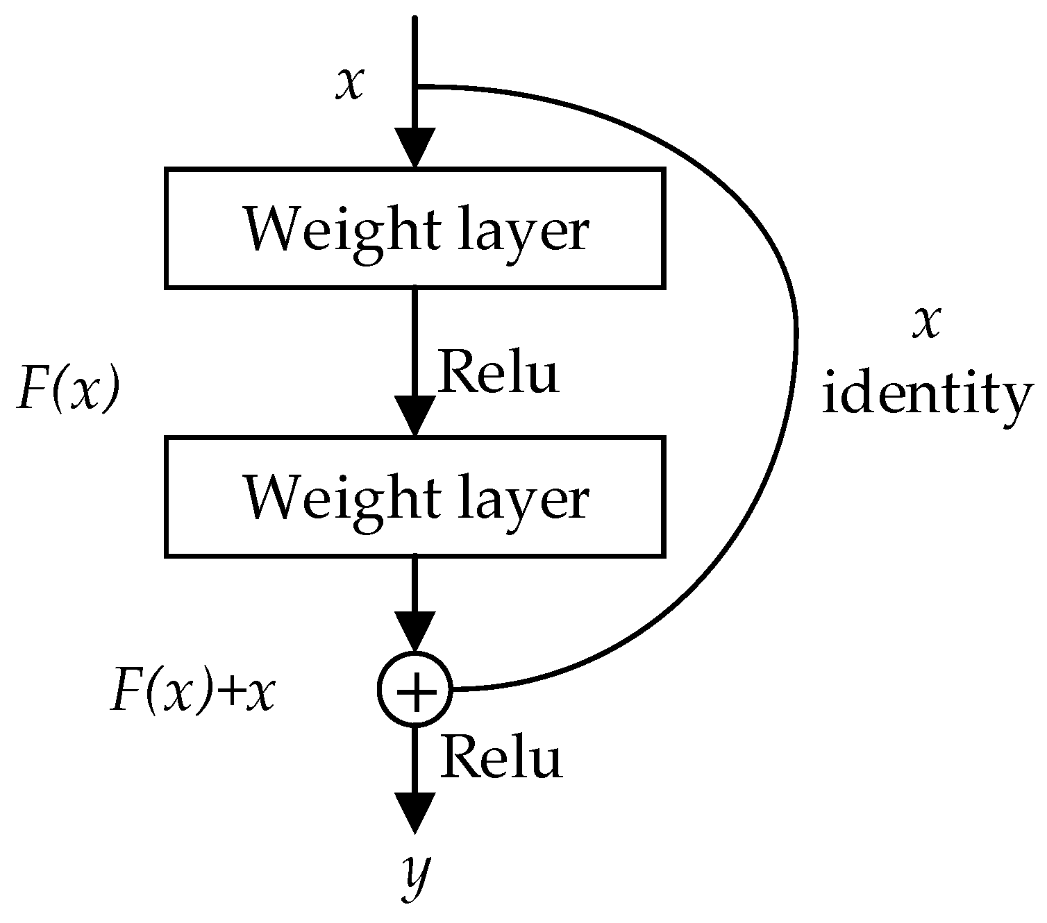
A deep residual network (ResNet) [34] is a deep network based on residual learning that won first place on the ImageNet Large Scale Visual Recognition Challenge 2015 (ILSVRC2015). Increasing the network depth of CNN can improve the accuracy of recognition and classification. At the same time, residual learning can solve the performance degradation caused by different network depths. In addition to the basic structure of general CNNs, ResNet also realizes residual learning by establishing cross-layer links between layers. A CNN shows the powerful ability of feature representation because it naturally integrates low-/middle-/high-level features and classifiers in an end-to-end multilevel manner. The “levels” of features can be enriched by the number of stacked layers (depth). However, a series of problems are caused by adding layers in the suitably deep model, such as vanishing/exploding gradients and higher training errors. ResNet, which introduces a deep residual learning framework (as shown in Figure 1), can maintain higher training accuracy as the depth of the network increases to hundreds of layers. Each unit can be explained by Equation (1):
where x and F(x) are the input and output vectors of the layers considered, respectively, and H(x) represents the residual mapping to be learned.

Figure 1.
Residual learning: a building block.
In this study, ResNet34 and ResNet50 networks were used for feature extraction. The structures of the two networks are shown in Table 1. The two networks include six blocks: Conv1, Conv2, Conv3, Conv4, Conv5, and Fc. As the name suggests, ResNet34 has 33 convolution layers and one fully connected layer, whereas ResNet50 includes 49 convolutional layers and one fully connected layer. For ResNet34, Conv1 consists of one convolution layer with a size of 7 × 7, a depth of 64, and a stride of 2. For Conv2, Conv3, Conv4, and Conv5, a stack of 2 layers is used in each residual function. The convolution kernel size of each stack is 3 × 3, and the depths are 64, 128, 256, and 512. Each block has a different number of stacks: 3, 4, 6, and 3. The size of the output characteristic map of Conv5 is 3 × 3 × 512. Finally, the Softmax function is adopted to classify the feature map of Conv 5, and the output is the category of classification. The convolution combination of ResNet50 is more complex, which uses a stack of 3 layers instead of 2 with each residual function. The three convolution kernels are 1 × 1, 3 × 3, and 1 × 1, respectively. The number of stacks in each block is similar to ResNet34. The output size of Conv5 of Resnet50 is 7 × 7 × 2048. In image registration, the registration feature is usually calculated using the eigenmatrix rather than the class value output by the fully connected network. Therefore, the output of the last convolution layer of Conv5 of ResNet34 and ResNet50 was used for feature fusion and registration.

Table 1.
ResNet network structure diagram of different depths.
3. Methodology
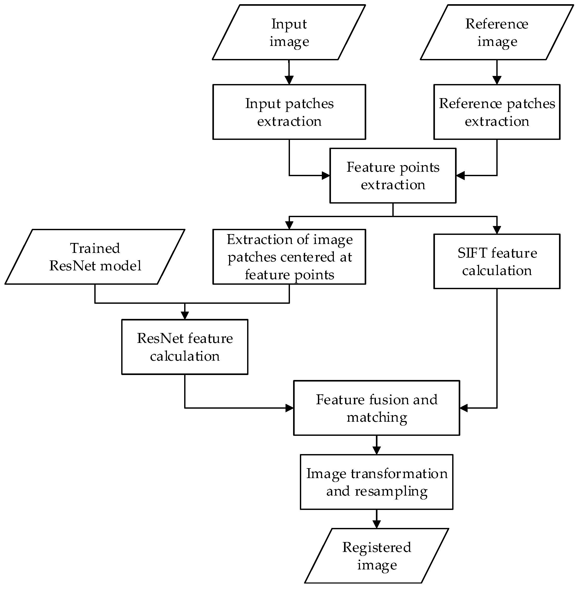
The proposed method fuses CNN and SIFT features to describe feature points obtained using the SSR method [35]. As shown in Figure 2, the proposed method consists of two major steps. The ResNet model was first trained to obtain a trained ResNet model, which was then used to extract ResNet features. Then, the combined SIFT and ResNet features were employed for image registration. The details are introduced in the following sections.
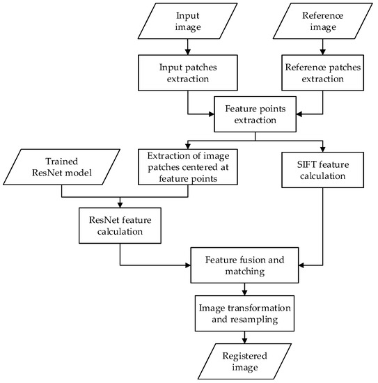
Figure 2.
The image registration flowchart for the combination of ResNet and SIFT.
3.1. Training of ResNet Model
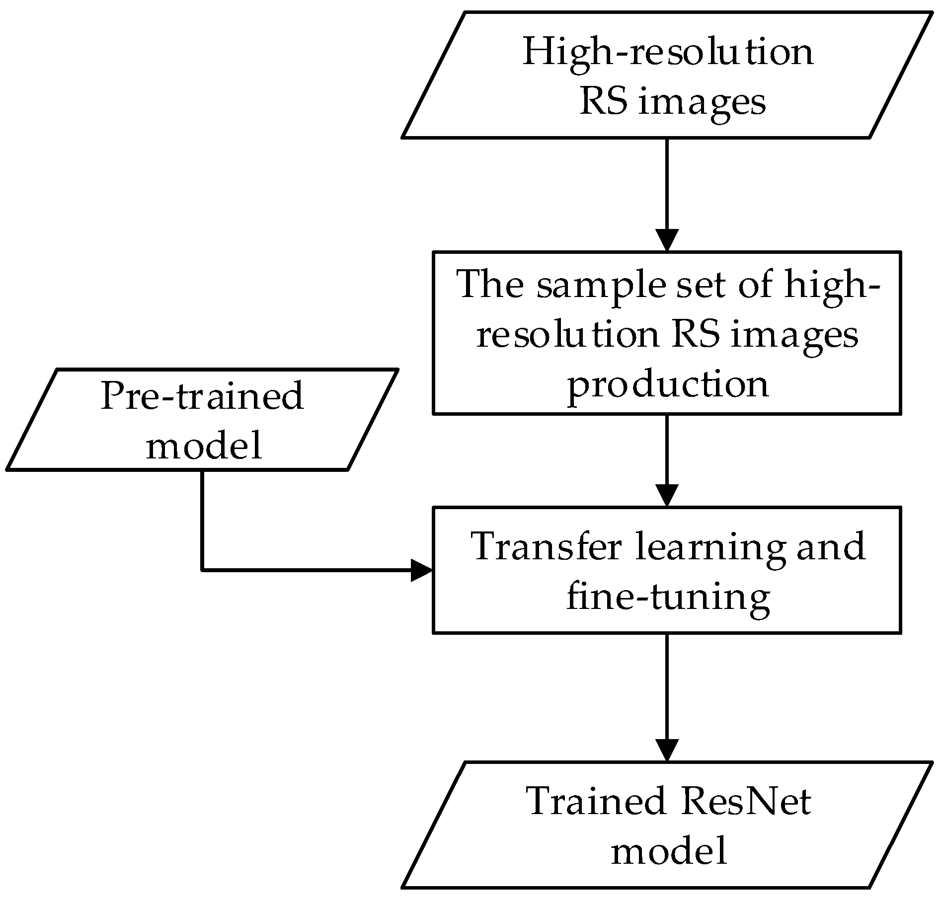
In this part, the sample set of HR remote sensing images was constructed, and the ResNet model suitable for image registration was constructed through transfer learning and fine-tuning. The training process of the ResNet model is shown in Figure 3.

Figure 3.
Training process of the ResNet model.
3.1.1. Sample Set of HR Remote Sensing Images
Similar to other CNN networks, ResNet is usually used for natural images, which cannot be directly applied in remote sensing image processing. Compared with natural images, HR remote sensing images has more complex image information. In addition, images from different sensors have different spectral widths and different number of bands. For example, the GaoFen (GF) images used have four spectral bands, whereas the Google Earth (GE) images used in this work have three spectral bands. Moreover, transfer learning was employed to solve the problem of a limited number of samples and improve efficiency. Therefore, it is necessary to perform image preprocessing when constructing a training sample set for multisource HR remote sensing images.
In this paper, the first three principal components were extracted by principal component analysis (PCA) for multisource satellite images to form new images with three bands. The PCA was selected for three reasons. First, as a data dimension reduction method, PCA can be used to obtain independent components of HR remote sensing images. Second, the first three principal components of PCA can preserve the major information shown in the original data to the maximum extent. Third, PCA is an unsupervised algorithm with less manual intervention and is easy to implement in practice.
Based on the images obtained from image preprocessing, the training sample set is created through two steps, namely, collecting sample image patch pairs with tie points and image transformation on the collected sample image patches. To obtain sample image patch pairs, this work follows the conventional algorithm to extract matched tie points and select the image patches centered on these points with a size of 64 × 64. Then, three types of random transformation (image scaling, rotation, and brightness transformation) were carried out for each image patch to expand the sample image patches. In this paper, a total of 253 image patch pairs were extracted, and 96 transformations, including 18 scaling and brightness transformations and 60 rotation transformations, were selected. The sample set of HR remote sensing images constructed in this paper only contains registered sample image patches. For each patch, the original image patch and the corresponding transformed image patches have the same label, which is regarded as a registration feature class. Therefore, a sample set of 253 classes, each class consisting of 194 (2 + 96 × 2) image patches, was constructed. At the same time, the training and testing sets were randomly split into 80% and 20%.
3.1.2. Transfer Learning and Fine-Tuning
A large number of sample images are needed for the training of CNNs to better describe the image features. However, a limited number of samples were available, as remote sensing images were used in this paper. Therefore, the ResNet models were trained through transfer learning and fine-turning, which can reduce the training time and improve the feasibility of the training model for new images.
Transfer learning is the process of taking a pretrained network as the initial state of the target network and then fine-tuning the target network using the target data [36]. Thus, the generalization performance of the target network is improved and dramatically reduces the training cost [37]. In this work, the pretrained ResNet model was obtained by training the ImageNet dataset [38]. ResNet models were finally obtained by fine-tuning the pretrained ResNet model using the stochastic gradient descent (SGD) algorithm and a sample set of HR remote sensing images. Fine-tuning aims to make the existing trained ResNet models more suitable for new images. Regarding the fine-tuning process, the input size, learning rate, momentum, weight decay, and iteration times were set as 64 × 64, 0.001, 0.9, 0.0005, and 10,000, respectively.
3.2. Image Registration Based on a Combination of SIFT and ResNet Features
The ResNet model obtained in Section 3.1 was used to combine the SIFT and ResNet features to complete the image registration based on the feature-based image registration method. This work consists of three steps, which are feature extraction based on an image partitioning strategy, feature fusion and matching, and image registration.
3.2.1. Feature Extraction Basedn Image Partitioning Strategy
For HR remote sensing images with a large size, feature detection usually requires a long computation time. Thus, to reduce the computation time and complexity, the proposed method adopts an image partitioning strategy [35]. This strategy considers geographic information of remote sensing images. First, n × n patches were obtained by cutting the input image, and the image coordinates of the four corners of each patch were recorded. Next, the image coordinates were transformed into the projected coordinates using a mapping relationship (Equation (2)). Then, the position of each patch in the reference image was located according to the previous step. Finally, the reference image of each patch was clipped from the entire reference image to form image patch pairs with the corresponding input image patches.
where (xi, yi) are the image coordinates of the ith pixel, and (Xi, Yi) are the corresponding projected coordinates of (Ii, Ji); (X0, Y0) are the projected coordinates of the top left corner in the original whole scene input image, and G1, G2, G3 and G4 are the parameters of the transformation model.
As described in Section 2.1, feature points were detected from image patch pairs by the Shi_Tomasi algorithm. For the Shi_Tomasi algorithm, we refer to [35] and set the maximum number of feature points for each image patch as 1500 in this work.
The SIFT feature descriptor uses local features at a low level, while the ResNet feature descriptor represents the features of the image at a deep level. Therefore, a more accurate feature descriptor can be obtained by combining the SIFT and ResNet feature descriptors. For each feature point P(x, y), the SIFT descriptor (denoted as fS) was first calculated. Then, the image patch centered on P(x, y) with a size of 64 × 64 was clipped from the input image. Finally, the image patch was taken as the input data of the trained ResNet model, and the output of the last convolution layer of the ResNet model (i.e., Conv5) were taken as the feature descriptor of the ResNet model, which is denoted as fC.
3.2.2. Feature Fusion and Matching
Due to the significant difference between the SIFT descriptor and the ResNet descriptor, the normalization operation must be applied to the two descriptors before combining the two descriptors. In this work, the Z-score normalization method was employed to normalize the two descriptors, respectively. Then, the cosine distance [Equation (3)] was applied to measure the similarity between the two candidate key points in the reference and input image:
where D (i, j) are the cosine similarity between i and j, the value range is [−1, 1]. i and j are candidate key points in the range of [1, n]. n is the number of feature points. fr and fw are feature descriptors of candidate key points in the reference image and the input image, respectively.
Finally, the similarity between the candidate key points was calculated by using Equation (4):
where Pr and Pw represent the candidate key points from the reference image and the input image, respectively. D (Pr, Pw) represents the cosine distance between feature vector Pr and feature vector Pw, while the DC (Pr, Pw), DS (Pr, Pw) and DF (Pr, Pw) represent the D (Pr, Pw) of ResNet, SIFT and the combination of ResNet and SIFT, respectively. In this work, the best bin first (BBF) algorithm was selected for feature-matching. A matched point is determined by calculating the ratio R of the distance of the nearest neighbor (DNN) to the distance of the second nearest neighbor (DSNN) (R = DNN/DSNN). R is greater than 0.9 in this work. Finally, the coordinates of each matching point need to be converted from image patch to the whole image scene [35].
To obtain matched tie points with even distribution, this work adopts a greedy algorithm [39] to remove redundant matched tie points. Start from a tie point with a small RMSE value, and if the distance between the point and the other points is less than the threshold, then the larger RMSE point is deleted as of a redundant control point. The operation was repeated until the end of the traversal.
3.2.3. Image Transformation and Resampling
The polynomial rectification model was used to warp the input image in this work. The coefficients of the polynomial model were solved using the matched tie points. After the coefficients were obtained, the input image was transformed and resampled to align it with the reference image.
4. Experiments and Results
In this section, we use five pairs of HR remote sensing images to evaluate the performance of the proposed method. The compared methods including the classical SIFT (hereafter referred to as SIFT), the advanced SIFT algorithm which adopts the same partitioning strategy as the proposed method (hereafter referred to as Patch-SIFT), and SURF. Section 4.1 describes the details of the five datasets. Then, the evaluation criteria are carried out in Section 4.2. Finally, Section 4.3 demonstrates the experimental results of the three methods.
All experiments were implemented under PyCharm 2019.3 (Python) for one PC with an Intel Core i7-8550U CPU 1.80-GHz processor. The physical memory of computer is 8.0 GB.
4.1. Datasets
Considering the differences in image size, terrain, and scene under different application conditions, two types of images were used in this work. The first is GaoFen satellite datasets with large sizes and covering urban and mountainous areas (Section 4.1.1). The other is HR satellite datasets with disaster information caused by severe earthquakes (Section 4.1.2). The registration accuracy of remote sensing images is important for earthquake disaster assessment and change detection.
4.1.1. Experiment 1: GaoFen Satellite Datasets
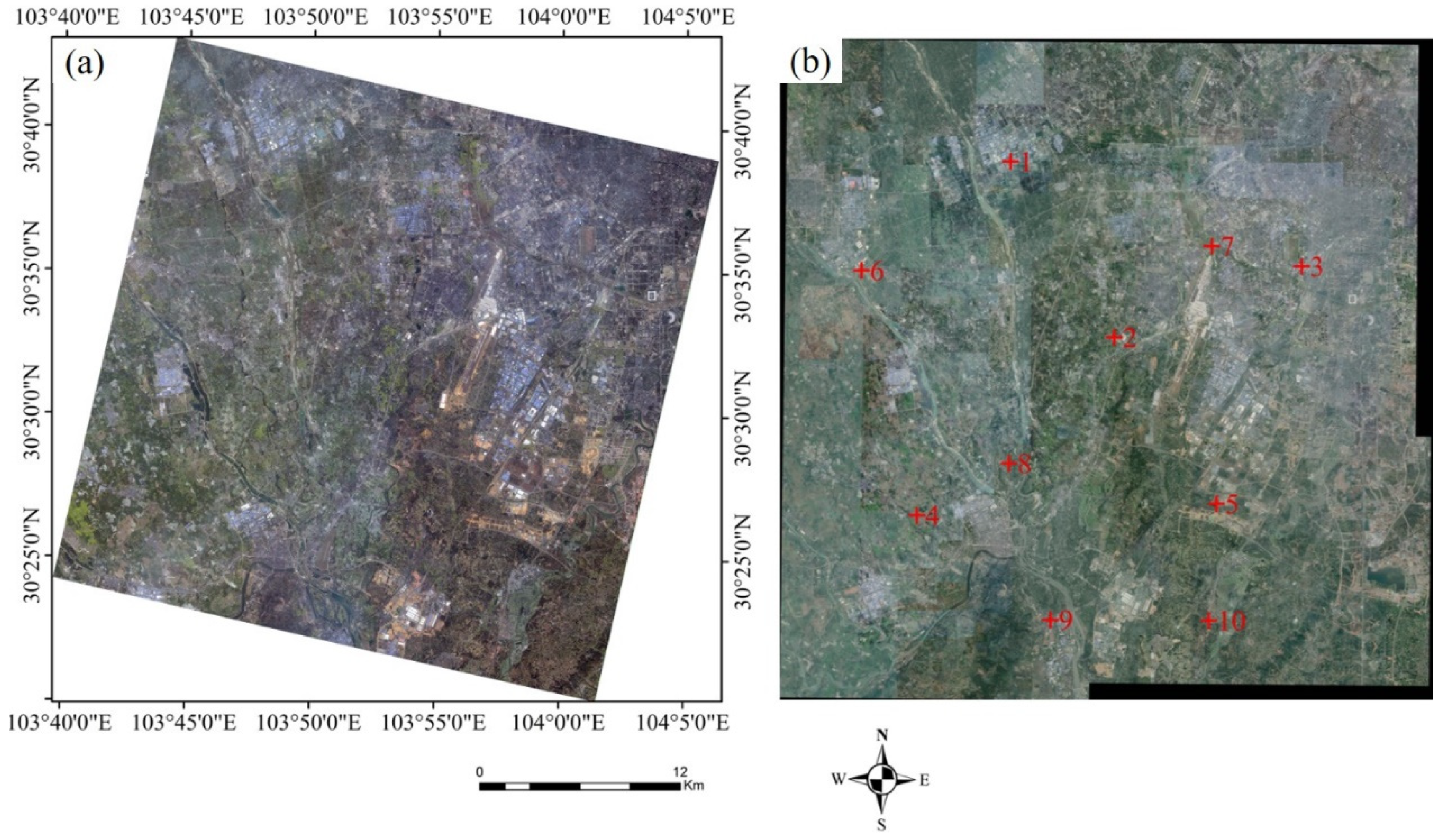
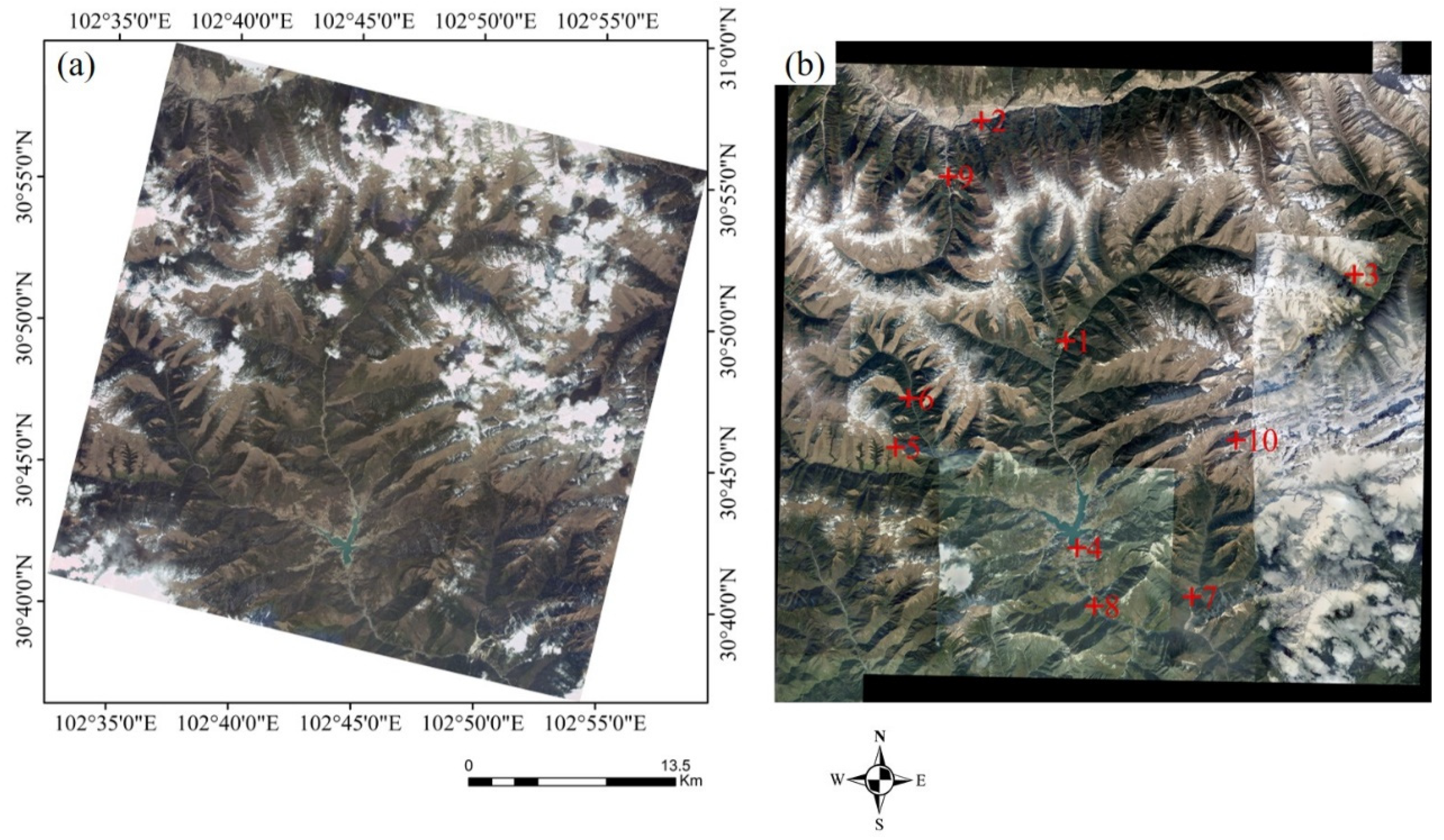
To verify the effectiveness of the proposed method in the registration of GaoFen remote sensing images, two sets of GaoFen-1 (GF-1) images covering urban (denoted as P-A) and mountainous areas (denoted as P-B) were used in the experiment. The multispectral images of GF-1 have a spatial resolution of 8 m. The GF-1 image of P-A, which covers the urban area of Chengdu, was acquired on 9 March 2018. The GF-1 image of P-B was recorded on 1 March 2018. It covers the mountainous area of Baoxing Town. In this work, Google Earth (GE) images were used as reference images. The details of GaoFen satellite remote sensing images and GE images are introduced in Table 2, and the images are shown in Figure 4a and Figure 5a. Due to the range of each input image being relatively large, it is difficult to obtain GE images recorded simultaneously. Therefore, we used GE images made from multiperiod coverage and mosaics as references.

Table 2.
Details of GaoFen multispectral images.

Figure 4.
GaoFen multispectral images of P-A. (a) GF-1 image (input image), (b) GE image (reference image). Points in red are verification points.

Figure 5.
GaoFen multispectral images of P-B. (a) GF-1 image (input image), (b) GE image (reference image). Points in red are verification points.
The characteristics of the two sets of images are that they all come from different sensors and different acquisition times, and the spectral differences between the input image and reference image are significant. In addition, the P-B covers a mountainous area with an average elevation of more than 3000 meters, and there is a small amount of cloud cover in the image. All of these factors increase the difficulty of automatic registration.
4.1.2. Experiment 2: HR Satellite Datasets with Disaster Information
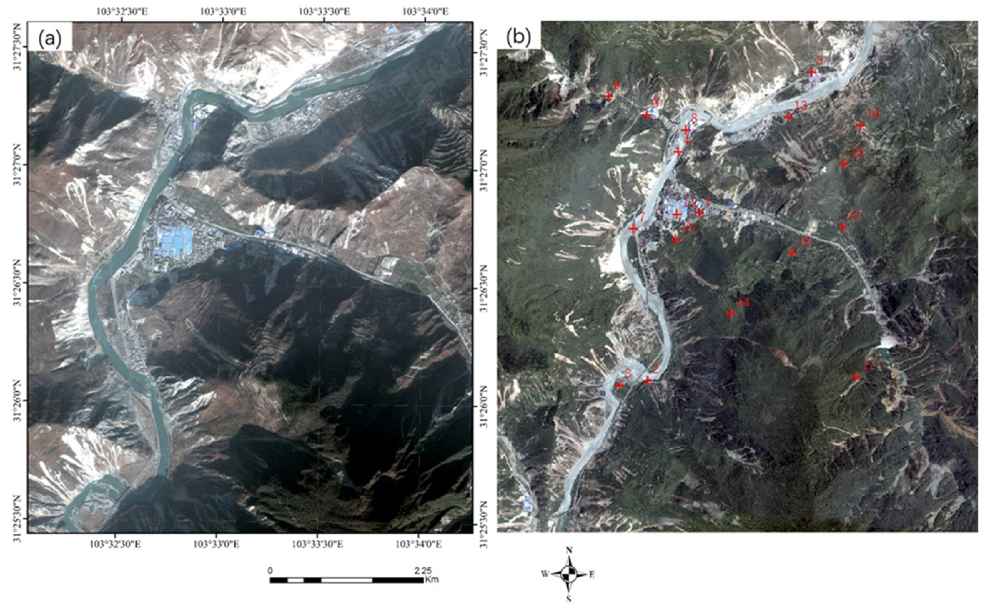
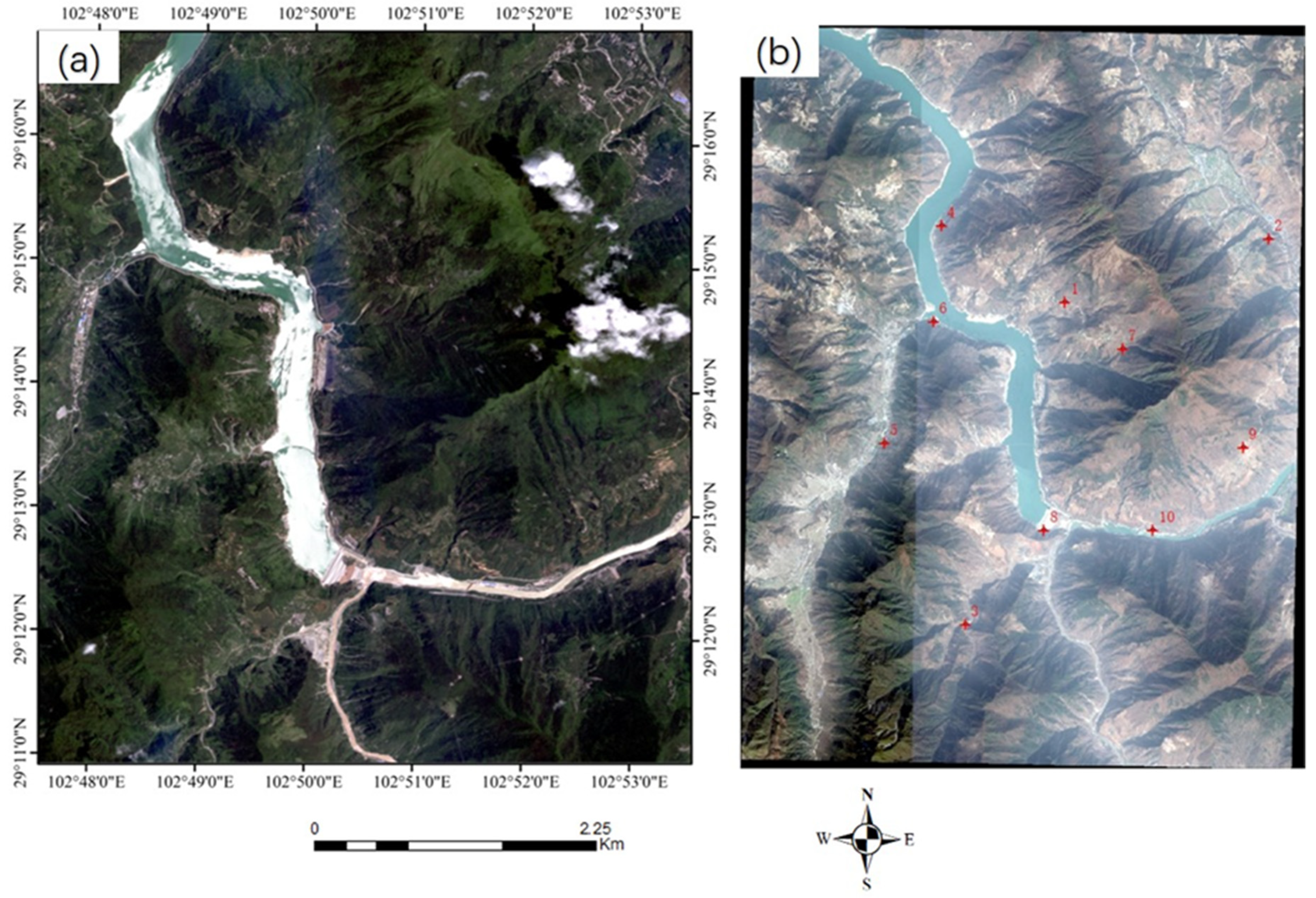
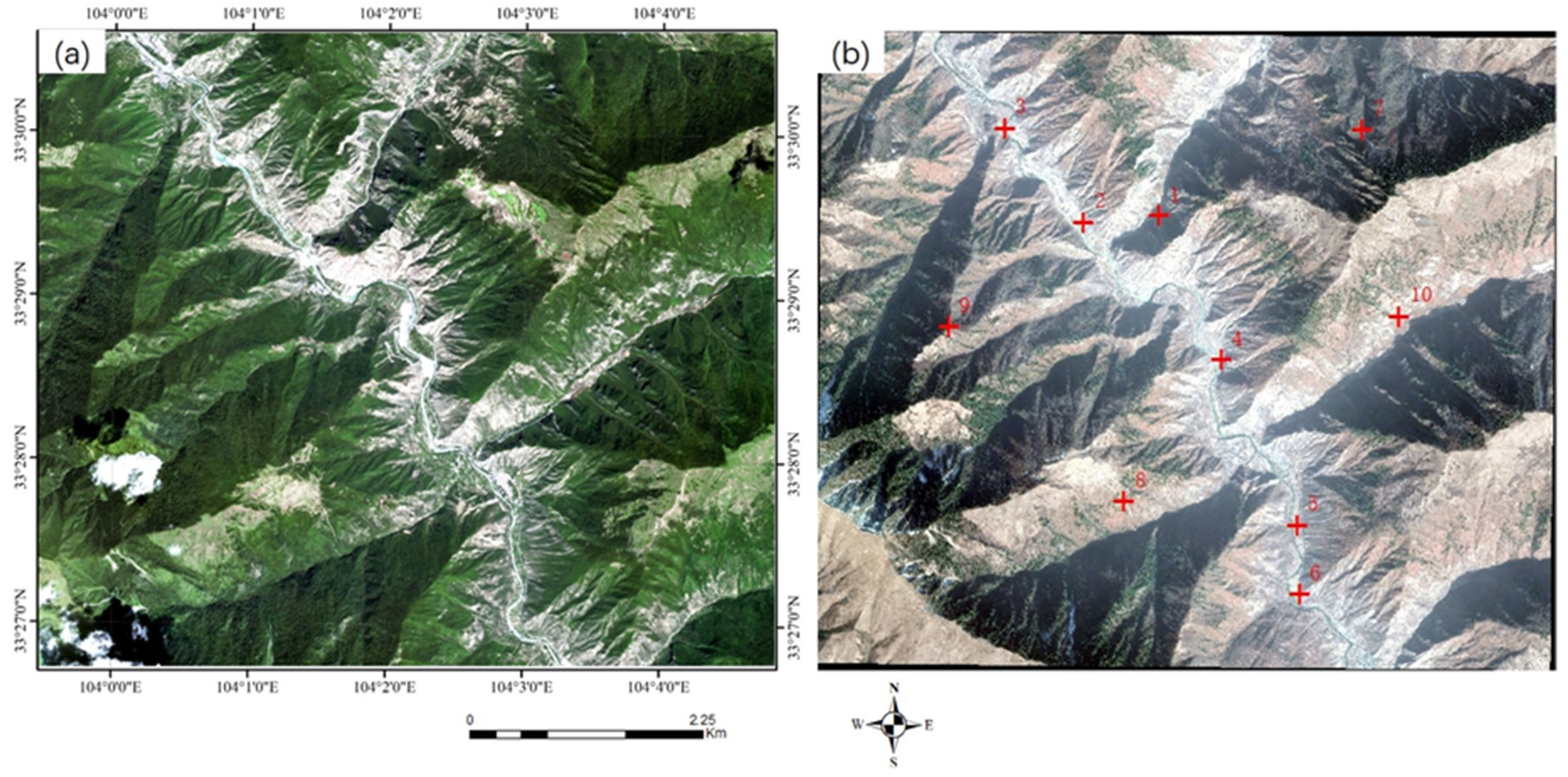
Both the accuracy and efficiency of automatic registration are crucial for rapid disaster assessment using remote sensing technology. Therefore, in addition to large HR images, three sets of HR remote sensing images containing different kinds of secondary disasters were employed to explore the applicability of the proposed method in different scenarios. The data details of the three sets denoted as P-C, P-D, and P-E are introduced in Table 3. The input image of P-C is a QuickBird multispectral image, which covers the landslides caused by the Wenchuan earthquake. The input image of P-D, which covers Baoxing Town, includes river expansion and landslides that suffered from the Yaan earthquake. The input image of P-E is a GaoFen-2 (GF-2) multispectral image. It covers the Jiuzhaigou area and contains landslides triggered by the Jiuzhaigou earthquake. Similarly, GE images were still used as reference images in this experiment. Secondary disasters can be observed from these images, as shown in Figure 6, Figure 7 and Figure 8.

Table 3.
Details of HR multispectral images with disaster information.

Figure 6.
HR multispectral images with disaster of P-C. (a) QuickBird image (input image), (b) GE image (reference image). Points in red are verification points.

Figure 7.
HR multispectral images with disaster of P-D. (a) GF-1 image (input image), (b) GE image (reference image). Points in red are verification points.

Figure 8.
HR multispectral images with disaster P-E. (a) GF-2 image (input image), (b) GE image (reference image). Points in red are verification points.
4.2. Evaluation Criteria
In this paper, five evaluation criteria [35,40] were adopted: number of matched tie points (Ncp), the time for registration (T), the transformation model accuracy obtained by the final tie points (RMSEM), root-mean-square based on the leave-one-out (LOO) method (RMSELoo), and geometric accuracy yielded using selected verification points (RMSET).
RMSEM, RMSELoo, and RMSET were calculated by Equation (5):
where (xi, yi) and (Xi, Yi) are the coordinates of the ith point on the reference image and after transformation, respectively. N is the number of matched tie points. The RMSEM is computed by all matched tie points, and RMSET is calculated by selected verification tie points, which were evenly distributed on ENVI. For RMSET, (Xi, Yi) corresponds to the reference image, whereas (xi, yi) is for the registered image. RMSELoo calculates the residual of tie points based on the leave-one-out method. For each tie point, the polynomial coefficients were estimated using the remaining N − 1 tie points and an RMSE was calculated. Finally, RMSELoo is the average RMSE of the N tie points.
4.3. Experimental Results
4.3.1. Experiment 1: GaoFen Multispectral Images
The statistical results of the four evaluation criteria introduced in Section 4.2 of the four methods for the two datasets are shown in Table 4. SIFT + ResNet34 and SIFT + ResNet50 represent the proposed method using a combination of SIFT and ResNet34 features and a combination of SIFT and ResNet50 features, respectively.

Table 4.
Registration results for GaoFen multispectral images.
Table 4 shows that SIFT + ResNet34 and SIFT + ResNet50 can achieve lower RMSE values than the compared methods for both urban areas (P-A) and mountainous areas (P-B). The proposed method using the combination of SIFT and ResNet34 (SIFT + ResNet34) has the lowest RMSE values, which are less than 0.5 pixels and 1 pixel for P-A and P-B, respectively. Compared with Patch-Sift and SIFT, the registration accuracy of the proposed method is improved by 0.22 and 0.23 pixels on average. For P-A, SIFT + ResNet34 yielded the largest number of tie points (Ncp = 184), which is obviously more than the compared methods (Ncp = 102, 116, 80, respectively). For P-B, SIFT + ResNet34 obtained 120 tie points, significantly more than the three compared methods. The Patch-SIFT yields 90 tie points, while SIFT and SURF only obtains 22 and 77 tie points, respectively. Although the Ncp obtained by the comparison method can satisfy the quadratic or cubic polynomial correction, incomplete registration exists in local areas due to the dispersed distribution of tie points. In addition, the running time of the proposed method is longer than the compared methods because the multilayer convolution of the ResNet network requires more time.
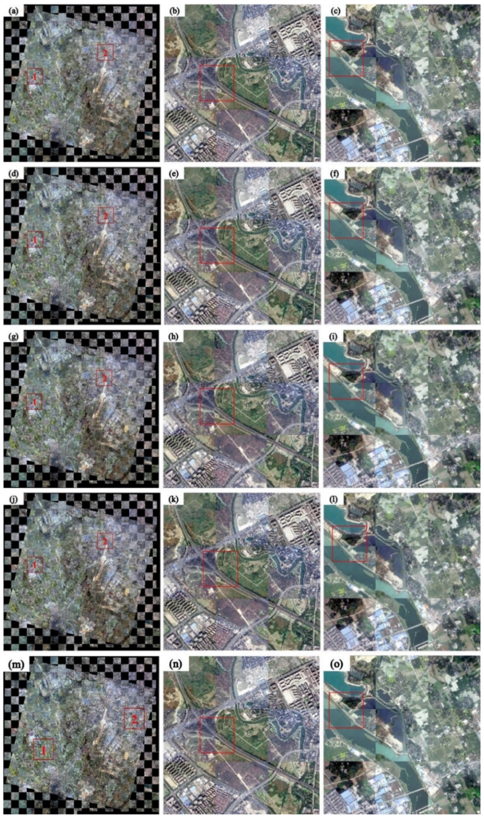
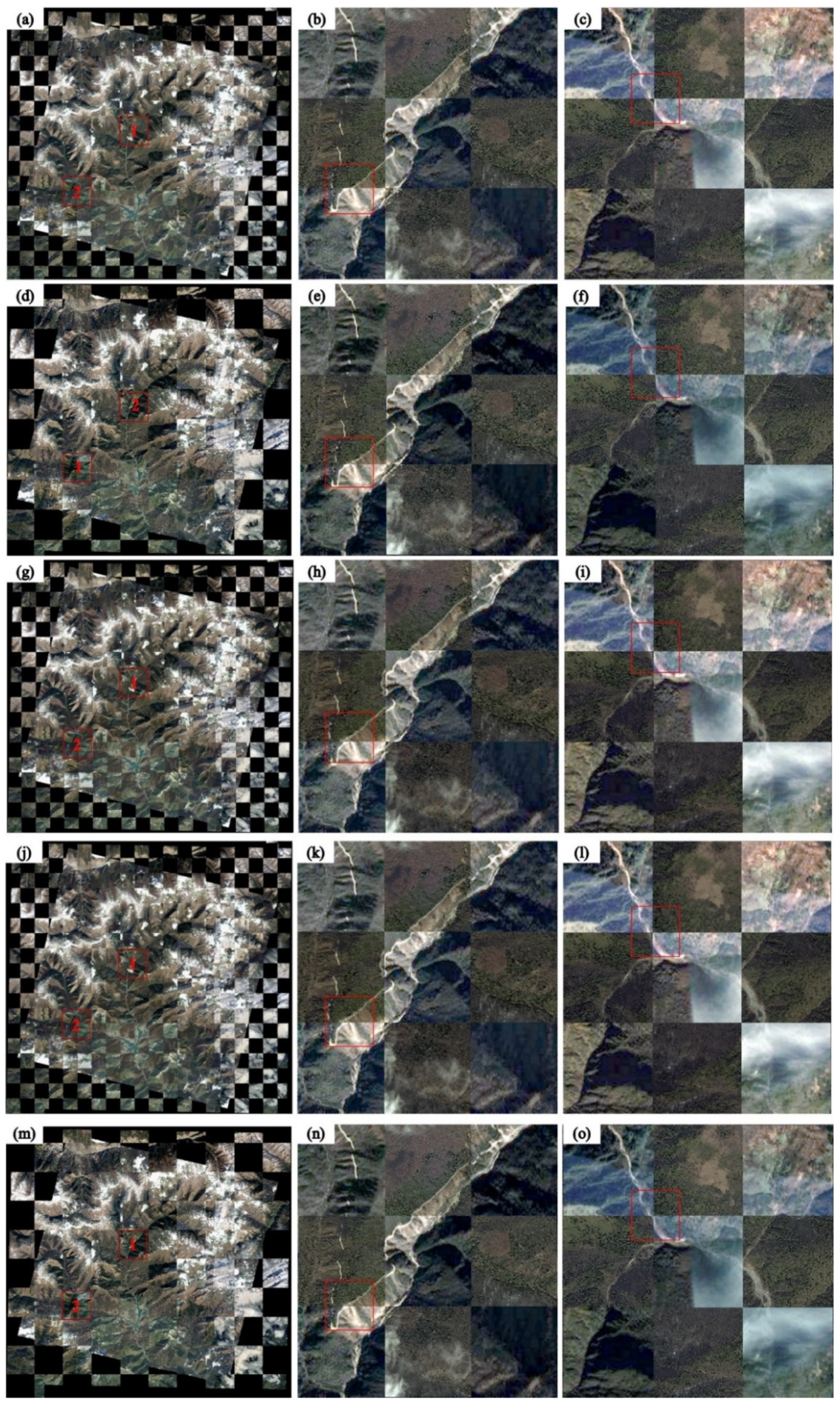
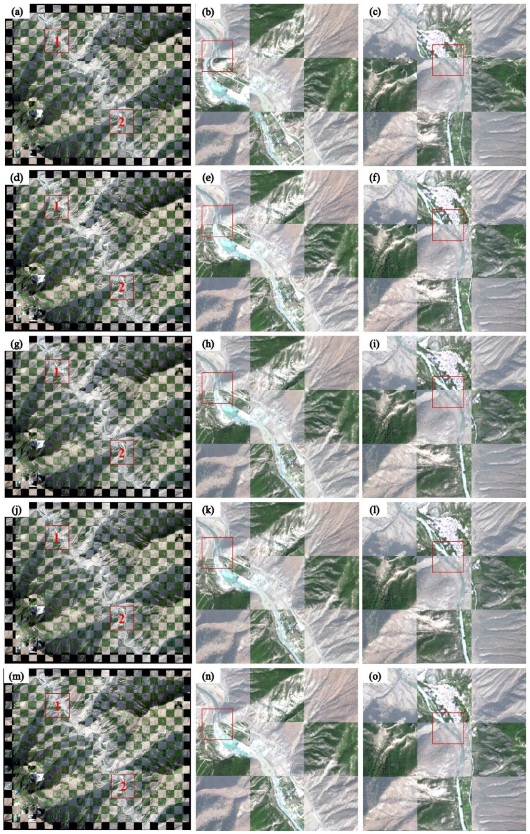
The registration results of the SIFT + ResNet34 and local details for the two sets are shown in Figure 9 and Figure 10, respectively. The registered image obtained by the proposed method (Figure 9d–o and Figure 10d–o) can effectively correct the deviations between roads, rivers in P-A, and mountains in P-B.
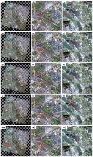
Figure 9.
Checkerboard images for the P-A dataset. (a) Original image; (b) enlarged image of red box 1 in (a); (c) enlarged image of red box 2 in (a); (d) result for the proposed method; (e) enlarged image of red box 1 in (d); (f) enlarged image of red box 2 in (d); (g) result for the Patch-SIFT; (h) enlarged image of red box 1 in (g); (i) enlarged image of red box 2 in (g); (j) result for the SIFT; (k) enlarged image of red box 1 in (j); (l) enlarged image of red box 2 in (j); and (m) result for the SURF; (n) enlarged image of red box 1 in (m); (o) enlarged image of red box 2 in (m). The red boxes indicate the regions where noticeable differences can be observed.

Figure 10.
Checkerboard images for the P-B dataset. (a) Original image; (b) enlarged image of red box 1 in (a); (c) enlarged image of red box 2 in (a); (d) result for the proposed method; (e) enlarged image of red box 1 in (d); (f) enlarged image of red box 2 in (d); (g) result for the Patch-SIFT; (h) enlarged image of red box 1 in (g); (i) enlarged image of red box 2 in (g); (j) result for the SIFT; (k) enlarged image of red box 1 in (j); (l) enlarged image of red box 2 in (j); and (m) result for the SURF; (n) enlarged image of red box 1 in (m); (o) enlarged image of red box 2 in (m). The red boxes indicate the regions where noticeable differences can be observed.
4.3.2. Experiment 2: HR Multispectral Images with Disaster Information
Table 5 shows the experimental results of HR multispectral images with disaster information. The RMSET values obtained by the proposed method were all less than 2 pixels. The lowest RMSET was achieved by SIFT + ResNet34, followed by SIFT + ResNet50.

Table 5.
Experimental results for HR multispectral images with disaster information.
In experiment 2, the SIFT method can hardly handle the image registration because of images containing different kinds of secondary disasters. For F-C, the SIFT + ResNet34 method provided 104 pairs of matched tie points, while the compared methods obtained 45, 21, and 12 tie points, respectively. The RMSET value of SIFT + ResNet34 is 1.69 pixels, which is improved 0.32, 7.49, and 0.74 pixels compared to the comparison method, respectively. For P-D, SIFT + ResNet34 extracted 31 tie points and yield 1.78 pixels RMSET. By contrast, the patch-SIFT and SIFT methods only extracted 9 and 4 tie points, providing RMSET values of 3.11 and 5.10 pixels, respectively. As the input image in P-D contains landslides and river expansion, SURF only obtains 4 tie points. Although the number of tie points is the same with that of the SIFT method, the RMSE of all tie points of the SURF method is too large to transform the input image. For P-E, the SIFT + ResNet34, Patch-SIFT, SIFT, and SURF methods provided 179, 94, 46, and 52 tie points, respectively. The RMSET yielded by the SIFT + ResNet34 method is lower than those obtained by the compared methods (1.14 pixels < 1.70 pixels < 1.88 pixels < 2.48 pixels). Although the SIFT method provided the lowest RMSEM values for P-C and P-E (0.81 pixels and 0.72 pixels, respectively), the corresponding RMSET values (9.18 pixels and 2.48 pixels, respectively) were high due to the small number of tie points and non-uniform distribution of tie points. In general, the RMSET of SIFT + ResNet34 improved by 0.80, 4.05, and 0.65 pixels on average. Similarly, the running time of the proposed method was obviously longer than those of the compared methods.
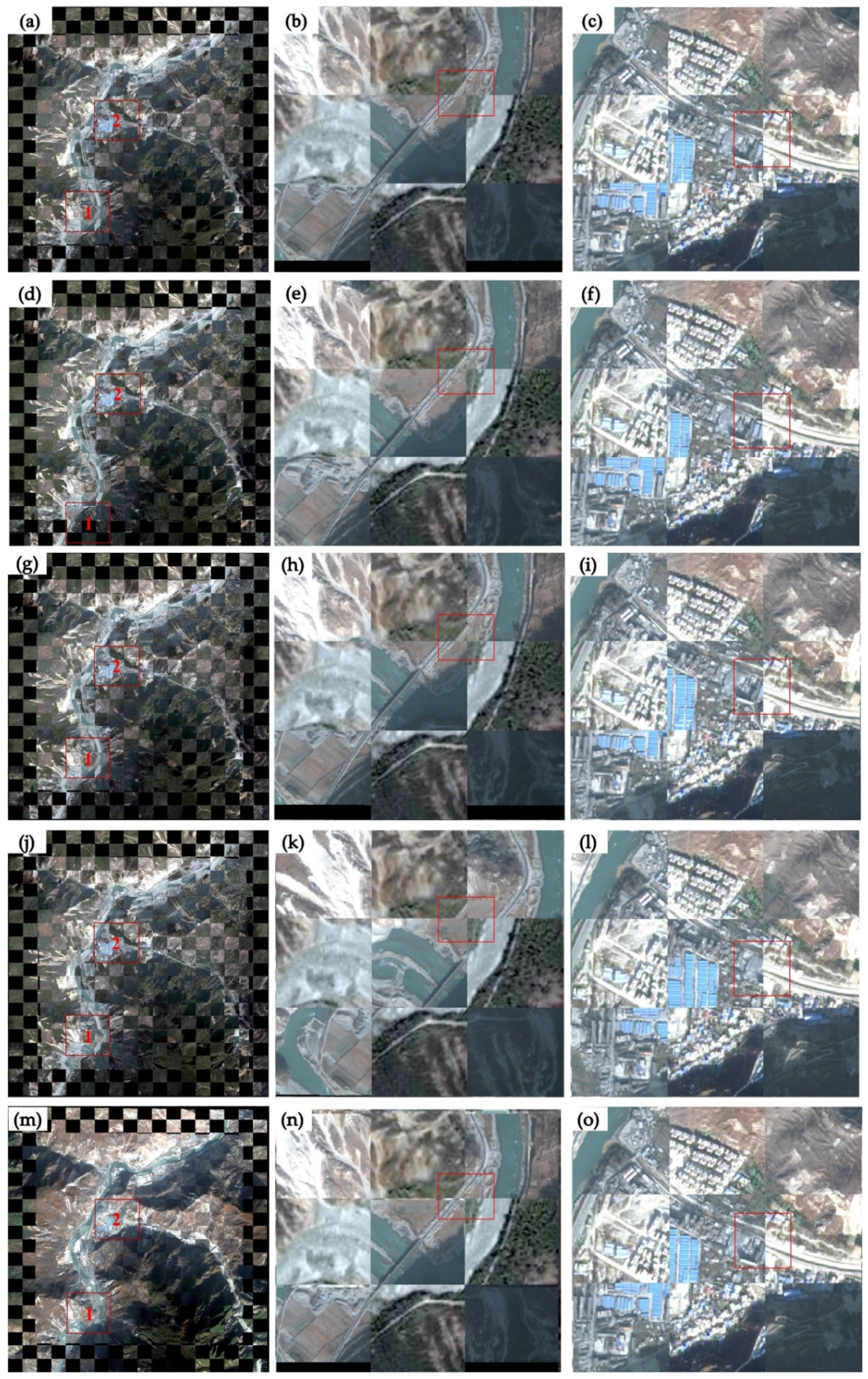
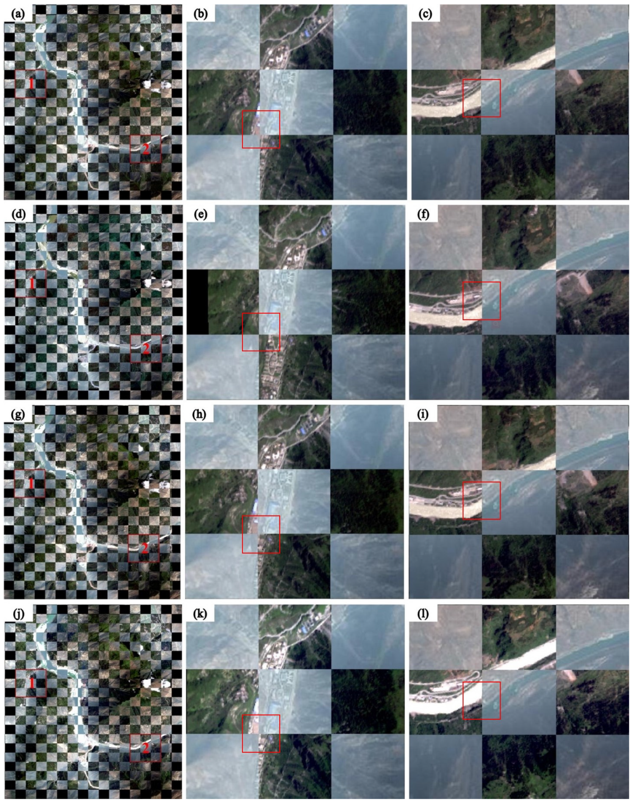
The registration results and local details for the three sets are shown in Figure 11, Figure 12 and Figure 13. Since the SURF method cannot yield a registered image for P-D, only the registration results of the other three methods were shown in Figure 12. The geometric position deviation of objects can be corrected by the proposed method in the registered image. Although the registered images produced by the SIFT + ResNet34 method show slight displacement for some roads (Figure 11e), houses (Figure 12e), and rivers (Figure 13f), SIFT + ResNet34 outperformed Patch-SIFT and SIFT.
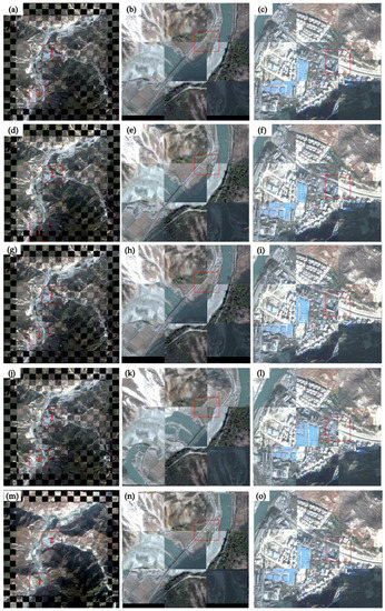
Figure 11.
Checkerboard images for the P-C dataset. (a) Original image; (b) enlarged image of red box 1 in (a); (c) enlarged image of red box 2 in (a); (d) result for the proposed method; (e) enlarged image of red box 1 in (d); (f) enlarged image of red box 2 in (d); (g) result for the Patch-SIFT; (h) enlarged image of red box 1 in (g); (i) enlarged image of red box 2 in (g); (j) result for the SIFT; (k) enlarged image of red box 1 in (j); (l) enlarged image of red box 2 in (j); and (m) result for the SURF; (n) enlarged image of red box 1 in (m); (o) enlarged image of red box 2 in (m). The red boxes indicate the regions where noticeable differences can be observed.
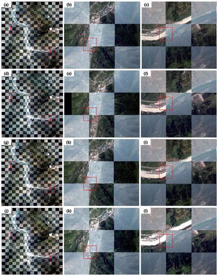
Figure 12.
Checkerboard images for the P-D dataset. (a) Original image; (b) enlarged image of red box 1 in (a); (c) enlarged image of red box 2 in (a); (d) result for the proposed method; (e) enlarged image of red box 1 in (d); (f) enlarged image of red box 2 in (d); (g) result for the Patch-SIFT; (h) enlarged image of red box 1 in (g); (i) enlarged image of red box 2 in (g); (j) result for the SIFT; (k) enlarged image of red box 1 in (j); (l) enlarged image of red box 2 in (j); and (m) result for the SURF; (n) enlarged image of red box 1 in (m); (o) enlarged image of red box 2 in (m). The red boxes indicate the regions where noticeable differences can be observed.
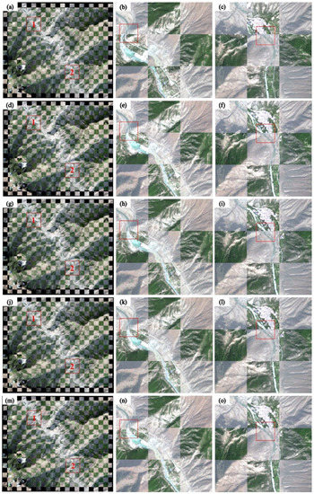
Figure 13.
Checkerboard images for the P-E dataset. (a) Original image; (b) enlarged image of red box 1 in (a); (c) enlarged image of red box 2 in (a); (d) result for the proposed method; (e) enlarged image of red box 1 in (d); (f) enlarged image of red box 2 in (d); (g) result for the Patch-SIFT; (h) enlarged image of red box 1 in (g); (i) enlarged image of red box 2 in (g); (j) result for the SIFT; (k) enlarged image of red box 1 in (j); (l) enlarged image of red box 2 in (j); and (m) result for the SURF; (n) enlarged image of red box 1 in (m); (o) enlarged image of red box 2 in (m). The red boxes indicate the regions where noticeable differences can be observed.
5. Discussion
The experimental results show that the proposed method can effectively improve registration accuracy by integrating high-dimensional ResNet features with conventional SIFT features. Compared with SIFT and patch-SIFT, the proposed method showed significant advantages in the number of matched tie points and accuracy. In the experiment using GaoFen multispectral remote sensing images, the RMSET of the urban area (P-A) was less than 0.5 pixels, and the RMSE of the mountain area (P-B) was less than 1 pixel. Meanwhile, for multisource remote sensing images with significant topographic relief and disaster information, the proposed method can effectively obtain better registered image.
In addition to the ResNet model, the VGG16 model was explored in combination with the SIFT feature. The output feature of the first fully connected layer (named FC6) was combined with SIFT; this was named SIFT + FC6, which was also evaluated using the two datasets introduced in Section 4.1.1 and compared to SIFT + ResNet34. The experimental results of SIFT + FC6 and SIFT + ResNet34, which yielded the best performance in Section 4.3, are shown in Table 6. As seen from the table, there was a slight difference in the registration accuracy between the two methods. However, SIFT + Resnet34 had a significant advantage in running time (T). For example, the running time of SIFT + ResNet34 for P-A was 41.65 s, which is only 32% of that of SIFT + FC6 (129.46 s). In general, the depth of networks greatly impacts the running time: the more convolution layers, the longer the running time. For example, SIFT + Resnet50 yielded a longer time than SIFT + Resnet34. The number of convolution layers of ResNet34 is approximately twice that of VGG16. However, the processing of the fully connected layer of VGG16 requires greater weight storage and runtime [41]. Therefore, compared with SIFT + FC6, SIFT + Resnet34 can provide faster registration speed.

Table 6.
Experimental results for different CNNs.
The weight for fusing the SIFT feature with the ResNet feature was set as a fixed value in this proposed method. This may not provide the optimal performance of some remote sensing images. Considering the different spectral characteristics of different images, setting the weight automatically according to different images to obtain the optimal registration performance is one way to improve future work. In addition, it takes a long time to extract high-dimensional features using a convolutional neural network. Therefore, it is necessary to improve the efficiency of feature extraction using convolutional neural networks in the future.
6. Conclusions
Traditional registration methods that only use low-level local features cannot meet the accuracy requirement of HR remote sensing images in complex terrain. A new registration method based on a deep residual network (ResNet) and SIFT was proposed to improve multisource remote sensing image registration accuracy. First, a sample set was constructed using registered HR remote sensing images. The ResNet model, which was pretrained by ImageNet, was then fine-tuned by the sample set. Then, based on the feature extraction algorithm, a combination of SIFT and ResNet features was constructed for image registration. In this work, two ResNets (ResNet34 and ResNet50) were selected to obtain combined features. These were denoted as SIFT + ResNet34 and SIFT + ResNet50, respectively. By using five pairs images, the accuracy and efficiency are compared with the traditional SIFT method and Patch-SIFT method. The RMSETs of the five pairs of HR images were all less than 2 pixels, and the RMSET of the urban area (P-A) was less than 0.5 pixels. Compared with SIFT, Patch-SIFT, and SURF, the number of tie points increased by 1.24–3.87 times, and the registration accuracy (RMSET) improved by 32.1–53.7%. The experimental results showed that the proposed method integrating deep-level ResNet features can effectively improve the registration accuracy of remote sensing images. The proposed method adopts the deep features of feature points to obtain accurate descriptors. This effectively increases the number of tie points and improves the registration accuracy. Meanwhile, the experimental results also indicated that the proposed method has better robust than the compared methods. The proposed method improves the registration performance of large-scale and HR images and meets the requirements of image registration in different applications, such as the registration of post-earthquake HR remote sensing images used for earthquake damage assessment.
Author Contributions
All authors made significant contributions to this work. X.Z. and H.L. designed the experiments and analyzed the datasets; X.Z. writing the original draft and edited the English text; H.L., L.J. and P.W. revised the manuscript. All authors read and agreed to the published version of the manuscript.
Funding
This research was funded by the Finance Science and Technology project of Hainan Province, China, grant number 418MS113, the National Natural Science Foundation of China, grant number 41801259, the Aerospace Information Research Institute, Chinese Academy of Sciences grant number Y951150Z2F, and the National Natural Science Foundation of China, grant number 41972308.
Institutional Review Board Statement
Not applicable.
Informed Consent Statement
Not applicable.
Conflicts of Interest
The authors declare no conflict of interest.
References
- Li, K.; Zhang, Y.; Zhang, Z.; Lai, G. A coarse-to-fine registration strategy for multi-sensor images with large resolution differences. Remote Sens. 2019, 11, 470. [Google Scholar] [CrossRef]
- Huang, F.; Mao, Z.; Shi, W. ICA-ASIFT-based multi-temporal matching of high-resolution remote sensing urban images. Cybern. Inf. Technol. 2016, 16, 34–49. [Google Scholar] [CrossRef][Green Version]
- Jiang, J.; Shi, X. A robust point-matching algorithm based on integrated spatial structure constraint for remote sensing image registration. IEEE Geosci. Remote Sens. Lett. 2016, 13, 1716–1720. [Google Scholar] [CrossRef]
- Ma, W.; Zhang, J.; Wu, Y.; Jiao, L.; Zhu, H.; Zhao, W. A novel two-step registration method for remote sensing images based on deep and local features. IEEE Trans. Geosci. Remote Sens. 2019, 57, 4834–4843. [Google Scholar] [CrossRef]
- Feng, R.; Shen, H.; BAI, J.; Li, X. Advances and opportunities in remote sensing image geometric registration: A systematic review of state-of-the-art approaches and future research directions. IEEE Geosci. Remote Sens. Mag. 2021, 3, 2–25. [Google Scholar] [CrossRef]
- Gong, M.; Zhao, S.; Jiao, L.; Tian, D.; Wang, S. A novel coarse-to-fine scheme for automatic image registration based on SIFT and mutual information. IEEE Trans. Geosci. Remote Sens. 2014, 52, 4328–4338. [Google Scholar] [CrossRef]
- Dawn, S.; Saxena, V.; Sharma, B.; Technology, I. Remote sensing image registration techniques: A survey. In Proceedings of the International Conference on Image and Signal Processing, Hong Kong, China, 12–15 September 2010; Springer: Berlin/Heidelberg, Germany, 2010; Volume 6134, pp. 103–112. [Google Scholar]
- Xiong, J.; Luo, Y.; Tang, G. An improved optical flow method for image registration with large-scale movements. Acta Autom. Sin. 2008, 34, 760–764. [Google Scholar] [CrossRef]
- Tu, Z.; Xie, W.; Zhang, D.; Poppe, R.; Veltkamp, R.C.; Li, B.; Yuan, J. A survey of variational and CNN-based optical flow techniques. Signal Process. Image Commun. 2019, 72, 9–24. [Google Scholar] [CrossRef]
- Moravec, H.P. Towards automatic visual obstacle avoidance. In Proceedings of the 5th International Joint Conference on Artificial Intelligence, Cambridge, MA, USA, 22–25 August 1977; pp. 584–590. [Google Scholar]
- Harris, C.G.; Stephens, M.J. A combined corner and edge detector. In Proceedings of the 4th Alvey Vision Conference, Manchester, UK, 31 August–2 September 1988; pp. 147–151. [Google Scholar]
- Shi, J.; Tomasi, C. Good features to track. In Proceedings of the IEEE Conference on Computer Vision and Pattern Recognition, New York, NY, USA, 21–23 June 1994; pp. 593–600. [Google Scholar]
- Lowe, D.G. Distinctive Image features from scale-invariant keypoints. Int. J. Comput. Vis. 2004, 60, 91–110. [Google Scholar] [CrossRef]
- Bay, H.; Ess, A.; TuytelAars, T.; Gool, L.V. Speeded-up robust feature (SURF). Comput. Vis. Image Underst. 2008, 110, 346–359. [Google Scholar] [CrossRef]
- Rosten, E.; Porter, R.; Drummond, T. Faster and better: A machine learning approach to corner detection. IEEE Trans. Pattern Anal. Mach. Intell. 2010, 32, 105–119. [Google Scholar] [CrossRef] [PubMed]
- Chen, S.; Zhong, S.; Xue, B.; Li, X.; Zhao, L.; Chang, C.I. Iterative scale-invariant feature transform for remote sensing image registration. IEEE Trans. Geosci. Remote Sens. 2021, 59, 3244–3265. [Google Scholar] [CrossRef]
- Mikolajczyk, K.; Schmid, C. Scale & affine invariant interest point detectors. Int. J. Comput. Vis. 2004, 60, 63–86. [Google Scholar]
- Heo, Y.S.; Lee, K.M.; Lee, S.U. Jiont depth map and color consistency estimation for stereo images with different illuminations and cameras. IEEE Trans. Pattern Anal. Mach. Intell. 2013, 35, 1094–1106. [Google Scholar]
- Huang, X.; Sun, Y.; Metaxas, D.; Sauer, F.; Xu, C. Hybrid image registration based on configural matching of scale-invariant salient region features. In Proceedings of the 2004 Conference on Computer Vision and Pattern Recognition Workshop (CVPR), Washington, DC, USA, 27 June–2 July 2004; p. 167. [Google Scholar]
- Hong, G.; Zhang, Y. Combination of feature-based and area-based image registration technique for high resolution remote sensing image. In Proceedings of the 2007 IEEE International Geoscience and Remote Sensing Symposium (IGASS), Barcelona, Spain, 23–28 July 2007; pp. 377–380. [Google Scholar]
- Teke, M. High-resolution multispectral satellite image matching using scale invariant feature transform and speeded up robust features. J. Appl. Remote Sens. 2011, 5, 053553. [Google Scholar] [CrossRef]
- Kupfer, B.; Netanyahu, N.S.; Shimshoni, I. An efficient SIFT-based mode-seeking algorithm for sub-pixel registration of remotely sensed images. IEEE Geosci. Remote Sens. Lett. 2015, 12, 379–383. [Google Scholar] [CrossRef]
- Zhao, X.; Zhang, Y. Fast image matching algorithm based on Harris corner point and SIFT. J. Lanzhou Univ. Technol. 2019, 45, 101–106. [Google Scholar]
- Simonyan, K.; Zisserman, A. Very deep convolutional networks for large-scale image recognition. In Proceedings of the 3rd International Conference on Learning Representations, ICLR 2015, San Diego, CA, USA, 7–9 May 2015; pp. 1–14. [Google Scholar]
- Chandrasekhar, V.; Lin, J.; Morère, O.; Goh, H.; Veillard, A. A practical guide to CNNs and Fisher Vectors for image instance retrieval. Signal Process. 2016, 128, 426–439. [Google Scholar] [CrossRef]
- Zhang, H.; Liu, X.; Yang, S.; Li, Y. Retrieval of remote sensing images based on semisupervised deep learning. J. Remote Sens. 2017, 21, 406–414. [Google Scholar]
- Liu, F.; Shen, T.; Ma, X. Convolutional neural network based multi-band ship target recognition with feature fusion. Acta Opt. Sin. 2017, 37, 248–256. [Google Scholar]
- Lee, W.; Sim, D.; Oh, S.J. A CNN-based high-accuracy registration for remote sensing images. Remote Sens. 2021, 13, 1482. [Google Scholar] [CrossRef]
- Han, X.; Leung, T.; Jia, Y.; Sukthankar, R.; Berg, A.C. MatchNet: Unifying feature and metric learning for patch-based matching. In Proceedings of the IEEE Conference on Computer Vision and Pattern Recognition, Boston, MA, USA, 7–12 June 2015; pp. 3279–3286. [Google Scholar]
- Zagoruyko, S.; Komodakis, N. Learning to compare image patches via Convolutional Neural Networks. In Proceedings of the IEEE Conference on Computer Vision and Pattern Recognition, Boston, MA, USA, 7–12 June 2015; pp. 885–894. [Google Scholar]
- Yang, T.Y.; Hsu, J.H.; Lin, Y.Y.; Chuang, Y.Y. Deepcd: Learning deep complementary descriptors for patch representations. In Proceedings of the IEEE International Conference on Computer Vision, Venice, Italy, 22–29 October 2017; pp. 3334–3342. [Google Scholar]
- Dame, A.; Marchand, E. Second-order optimization of mutual information for real-time image registration. IEEE Trans. Image Proc. 2012, 21, 4190–4203. [Google Scholar] [CrossRef] [PubMed]
- Fischiled, M.A.; Bolles, R.C. Random sample consensus-a paradigm for model-fitting with applications to image-analysis and automated cartography. Commun. ACM 1981, 24, 381–395. [Google Scholar]
- He, K.; Zhang, X.; Ren, S.; Sun, J. Identity mappings in deep residual networks. In Lecture Notes in Computer Science, Proceedings of the 14th European Conference, Amsterdam, The Netherlands, 11–14 October 2016; Springer nature: Basingstoke, UK, 2016; Volume 9908, pp. 630–645. [Google Scholar]
- Zhao, X.; Li, H.; Wang, P.; Jing, L. An image registration method for multisource high-resolution remote sensing images for earthquake disaster assessment. Sensors 2020, 20, 2286. [Google Scholar] [CrossRef] [PubMed]
- Wang, S.; Quan, D.; Liang, X.; Ning, M.; Guo, Y.; Jiao, L. A deep learning framework for remote sensing image registration. ISPRS J. Photogramm. Remote Sens. 2018, 145, 148–164. [Google Scholar] [CrossRef]
- Yosinski, J.; Clune, J.; Bengio, Y.; Lipson, H. How transferable are features in deep neural networks? In Proceedings of the 27th International Conference on Neural Information Processing Systems, Montreal, QC, Canada, 8–13 December 2014; MIT Press: Cambridge, MA, USA, 2014; Volume 2, pp. 3320–3328. [Google Scholar]
- Krizhevsky, A.; Sutskever, I.; Hinton, G.E. ImageNet classification with deep convolutional neural networks. In Proceedings of the 27th International Conference on Neural Information Processing Systems, Montreal, QC, Canada, 8–13 December 2014; MIT Press: Cambridge, MA, USA, 2012; pp. 1097–1105. [Google Scholar]
- Paul, S.; Pati, U.C.; Member, S. Remote sensing optical image registration using modified uniform robust SIFT. IEEE Geosci. Remote Sens. Lett. 2016, 13, 1300–1304. [Google Scholar] [CrossRef]
- Goncalves, H.; Goncalves, J.A.; Corte-Real, L. Measures for an objective evaluation of the geometric correction process quality. IEEE Geosci. Remote Sens. Lett. 2009, 6, 292–296. [Google Scholar] [CrossRef]
- He, K.; Zhang, X.; Ren, S.; Sun, J. Deep residual learning for image recognition. In Proceedings of the IEEE Conference on Computer Vision and Pattern Recognition, Las Vegas, NV, USA, 27–30 June 2016; pp. 770–778. [Google Scholar]
Publisher’s Note: MDPI stays neutral with regard to jurisdictional claims in published maps and institutional affiliations. |
© 2021 by the authors. Licensee MDPI, Basel, Switzerland. This article is an open access article distributed under the terms and conditions of the Creative Commons Attribution (CC BY) license (https://creativecommons.org/licenses/by/4.0/).

