Novel Intelligent Spatiotemporal Grid Earthquake Early-Warning Model

Abstract

The integration analysis of multi-type geospatial information poses challenges to existing spatiotemporal data organization models and analysis models based on deep learning. For earthquake early warning, this study proposes a novel intelligent spatiotemporal grid model based on GeoSOT (SGMG-EEW) for feature fusion of multi-type geospatial data. This model includes a seismic grid sample model (SGSM) and a spatiotemporal grid model based on a three-dimensional group convolution neural network (3DGCNN-SGM). The SGSM solves the problem concerning that the layers of different data types cannot form an ensemble with a consistent data structure and transforms the grid representation of data into grid samples for deep learning. The 3DGCNN-SGM is the first application of group convolution in the deep learning of multi-source geographic information data. It avoids direct superposition calculation of data between different layers, which may negatively affect the deep learning analysis model results. In this study, taking the atmospheric temperature anomaly and historical earthquake precursory data from Japan as an example, an earthquake early warning verification experiment was conducted based on the proposed SGMG-EEW. Five groups of control experiments were designed, namely with the use of atmospheric temperature anomaly data only, use of historical earthquake data only, a non-group convolution control group, a support vector machine control group, and a seismic statistical analysis control group. The results showed that the proposed SGSM is not only compatible with the expression of a single type of spatiotemporal data but can also support multiple types of spatiotemporal data, forming a deep-learning-oriented data structure. Compared with the traditional deep learning model, the proposed 3DGCNN-SGM is more suitable for the integration analysis of multiple types of spatiotemporal data.

1. Introduction

Spatiotemporal big data analysis is a hot topic in the field of geospatial information. Recently, deep learning has provided a solution for the pattern recognition of a single type of geospatial data, such as land-use classification based on optical remote sensing image data [1,2,3]. However, it is typically necessary to use multiple data types. For example, in the analysis of earthquake precursors, the data concerning the time and space of earthquakes include atmospheric anomalies and historical earthquakes. Multi-type geospatial information integration analysis challenges the existing spatiotemporal data organization model and the analysis model based on deep learning.

Before the popularization of big data, the standard methods primarily included earthquake warnings based on earthquake mechanisms, mechanical models, and earthquake precursor analysis using statistics. For example, UCERF [4], which established a fault model for California in the United States, is based on earthquake mechanisms. The attributes of each study-area raster grid cell are a series of mechanical and statistical characteristics based on the fault model. However, UCERF only provides the possibility of earthquake occurrence on a very rough time scale (~10 years), showing the complexity of earthquake mechanical mechanisms. By analyzing the spatiotemporal correlation between earthquakes and their possible precursors, the relationship between them was established and then an earthquake warning system was developed. The earliest work in this field was the Gutenberg–Richter (GR) law [5]. This model gives the relationship between a certain magnitude threshold and the total number of earthquakes with magnitudes exceeding the threshold in a specific region and time. The GR law shows a strong correlation between earthquakes and historical earthquakes, thus the historical earthquakes can be the precursors of new earthquakes in the same region. The parameter b of the GR law is an important statistical feature. Some follow-up studies have further designed statistical features on the basis of parameter b, assigning these statistical features to each grid cell on the basis of raster data organization and used historical earthquakes to predict new earthquakes [6] or used the data of the main shock to predict possible aftershocks [7].

Some researchers have also combined a model based on earthquake mechanisms with a model based on statistics. The representative literature in this field is Zhou et al. [8]. Based on historical earthquake data, the author carried out further feature engineering on the earthquake catalog with a dynamic model. Taking the average value of the earthquake time interval and earthquake magnitude as the input information, statistical machine learning methods, such as the support vector machine (SVM), can be used for earthquake early warning. In recent years, studies of earthquake prediction based on statistics have found that the geographical phenomena with strong spatiotemporal correlation with earthquakes include not only historical earthquakes but also geothermal anomalies [9], geomagnetic anomalies [10], and atmospheric anomalies [11]. However, unlike earthquakes and historical earthquakes, the statistical relationship between these spatiotemporal phenomena and earthquakes has not been established as the general formula of the GR law, which is not suitable for the raster data model that requires statistical characteristics as grid attributes. The data are arranged according to a hierarchical organizational model based on a vector point model. Therefore, these studies primarily analyze the original earthquake and its precursor data, and the data organization is based on the hierarchical organization model of the vector point.

Research on earthquake prediction based on the traditional non-deep learning analysis model shows a highly non-linear spatiotemporal correlation between earthquake precursors and earthquakes, and a more complex analysis model can improve earthquake early warning reliability. Therefore, in recent years, with the emergence of deep learning with higher model complexity, many studies are exploring deep learning for earthquake prediction. In a study by Alves [12] based on historical earthquake data, some indexes, such as the moving average of historical earthquake times, are designed as inputs and the fully connected neural network (FCNN) is used for earthquake prediction. The predicted earthquake was accurate to the space area with a longitude–latitude span of approximately 2° and a time window with a time span of approximately one year. The difference between the predicted and actual magnitudes was approximately a value of one. Based on historical earthquakes and the GR law, various characteristics reflecting seismic mechanical properties, energy, and time distribution were designed as inputs in studies by Asencio-Cortés et al. [13] and Reyes et al. [14], and FCNN was used for earthquake prediction. The desired prediction concerned whether two cities in Chile would have an earthquake of a magnitude of >4.5 in a five-day time window. Devries et al. [15] did not use historical earthquakes but designed a series of mechanical characteristics based on the fault zone model as the input of the FCNN to predict aftershocks in each 5 km × 5 km sub-region of areas where major earthquakes have occurred. The prediction accuracy index of the experimental results reached an AUC of 0.85. In earthquake predictions using FCNN, the researchers primarily studied the relationship between earthquakes and historical data and used a hierarchical model based on vector point objects to organize the spatiotemporal data of earthquakes. Mosavi et al. [16] used historical earthquake data from Iran and a radial basis function neural network to predict the time interval of large earthquakes in this dataset. Asencio-Cortés et al. [17] used historical earthquake data from Japan and FCNN to predict whether an earthquake with a magnitude of >5 would occur within seven days. The results showed that the prediction accuracy of FCNN was higher than that of some traditional machine learning methods, such as SVM and K-nearest neighbor.

In a study by Panakkat and Adeli [18], in addition to FCNN, the input historical earthquake data were organized and entered into the recurrent neural network (RNN) according to the time sequence to predict the maximum earthquake magnitude likely to occur in the next month at specific locations. The experiment revealed that RNN’s prediction ability was better than FCNN’s in this case. The seismic features used by Panakkat and Adeli [18], Asencio-Cortés et al. [13], and Reyes et al. [14] are different. Martínez-Álvarez et al. [19] analyzed the importance of different features in earthquake prediction using FCNN and seismic data from Chile and the Iberian Peninsula. It was found that these features had a similar order of importance in the two different study areas and the feature based on the GR law was the most important. In a study by Asim and Martínez-Álvarez [20], historical earthquakes and RNN were used to predict whether earthquakes with magnitudes of >5.5 would occur within the next month in the Hindu Kush Mountains and the prediction accuracy reached 71% in the test set. In Wang et al. [21], historical earthquake data were input into a long short-term memory (LSTM) network, that is, an improved RNN. Earthquake prediction was based on two simulation datasets. The above-mentioned earthquake prediction using RNN was primarily based on the hierarchical model of vector point objects to organize the spatiotemporal data of earthquakes. Huang et al. [22] organized the historical earthquake data of the entire Taiwan Province using the raster model. The study area was divided into 256 × 256 square sub-regions. The accumulated data of every 120 days formed a 256 × 256 raster map and the value of each raster grid represented the maximum magnitude of the corresponding sub-region over the past 120 days. Convolution neural networks (CNNs) can predict whether earthquakes with magnitudes of >6 will occur in the Taiwan Province over the next 30 days. The R-score was used to evaluate the prediction accuracy and the R-score of the prediction model was approximately 0.3. Although far from ideal, the accuracy of the earthquake prediction (R-score is close to 1) is significantly higher than that obtained using random input data (R-score is 0.065).

Compared with the use of historical earthquakes to predict new earthquakes, research on earthquake prediction based on atmospheric anomalies is still in its infancy and primarily focuses on the statistical correlation between different types of atmospheric anomalies and earthquakes. Shah et al. [23] conducted a correlation analysis between three large earthquakes (magnitude of 6 or above) in Pakistan and Iran, and the atmospheric observation data at that time. It was found that there were significant anomalies in different atmospheric parameters, including long-wave radiation, surface temperature, and nitrogen dioxide, which could be observed in a minimum of 5 days and a maximum of 21 days before the earthquake. However, the time difference between the anomalies and earthquake occurrence shows conspicuous differences in different areas. In Fujiwara et al. [11], 29 earthquakes with magnitudes of >4.8 in Japan and the atmospheric observation data at that time were analyzed, and it was found that these earthquakes had a strong correlation with the electromagnetic wave anomalies in the five days before the earthquake.

Deep learning can automatically learn and extract characteristics from the original data and CNN, a representative deep learning model, uses a spatial window to explore the spatial association information between data [24], which is suitable for grid data. In earthquake precursor analysis, deep learning analysis of the earthquake precursor based on multi-layer and multi-source spatial data is in its early stages and there is little related research. The deep learning frontier for multi-layer data is concentrated around traditional computer vision and remote sensing data analysis. With non-uniform multi-layer input gridded data, the existing methods primarily design the branch structure of the CNN, in which each branch network processes a layer and the results of different branches are summarized at the neural network’s end. Land-use classification based on multi-source remote sensing data [25,26] is a typical challenge. Chen et al. [27] designed a CNN with two branches to process and integrate multispectral optical remote sensing image data and (light detection and ranging) LiDAR data. Xu et al. [28] designed a CNN with three branches to process and integrate the hyperspectral remote sensing image, digital elevation model, and LiDAR data for land-use classification. Ienco et al. [29] designed a CNN with four branches to fuse the multi-temporal remote sensing image data of Sentinel-1 and Sentinel-2 satellites. In Hang et al. [30], a CNN with two branches was designed to fuse hyperspectral and LiDAR remote sensing images, and parameter-sharing technology was used for some parameters of the two branches, reducing the complexity of the model. Hong et al. [31] summarized the design ideas of branching neural networks in several studies and proposed that different branches of the neural network adopt different architectures. For example, one branch could use FCNN and the other branch could use CNN.

For the branching CNN for multi-layer data integration, the data matrix and data unit sizes can differ on different branches and there is no direct superposition between layer features on different branches. However, the structure of a branching neural network is complex. More data layers mean more branches and a more complex model. Therefore, the branch network is unsuitable for earthquake prediction involving multiple data types. Compared with a branching neural network, the structure of a neural network with only one backbone is simple and the costs of both network design and calculation are low. However, using a single backbone neural network for multi-layer data analysis requires overcoming the problems of correspondence between the different layers in data organization and feature integration of multi-source data in the analysis. Regarding data organization, for multi-layer data, the input data of CNN is block data with a unified matrix structure (layer number C, image height H, image width W). The data matrix formed by the different layers should be consistent in the H and W dimensions. Therefore, in terms of data organization, the gridding of different vector layers requires the different layers to form a unified H and W. This creates a relationship between the upper and lower layers, and a single-layer data slice can then form a multi-layer data block. Concerning data analysis, the calculation results of different layers are superimposed in the CNN. When different layers represent different data types, the data of different layers have different meanings. Therefore, this type of direct superposition is meaningless and should be avoided.

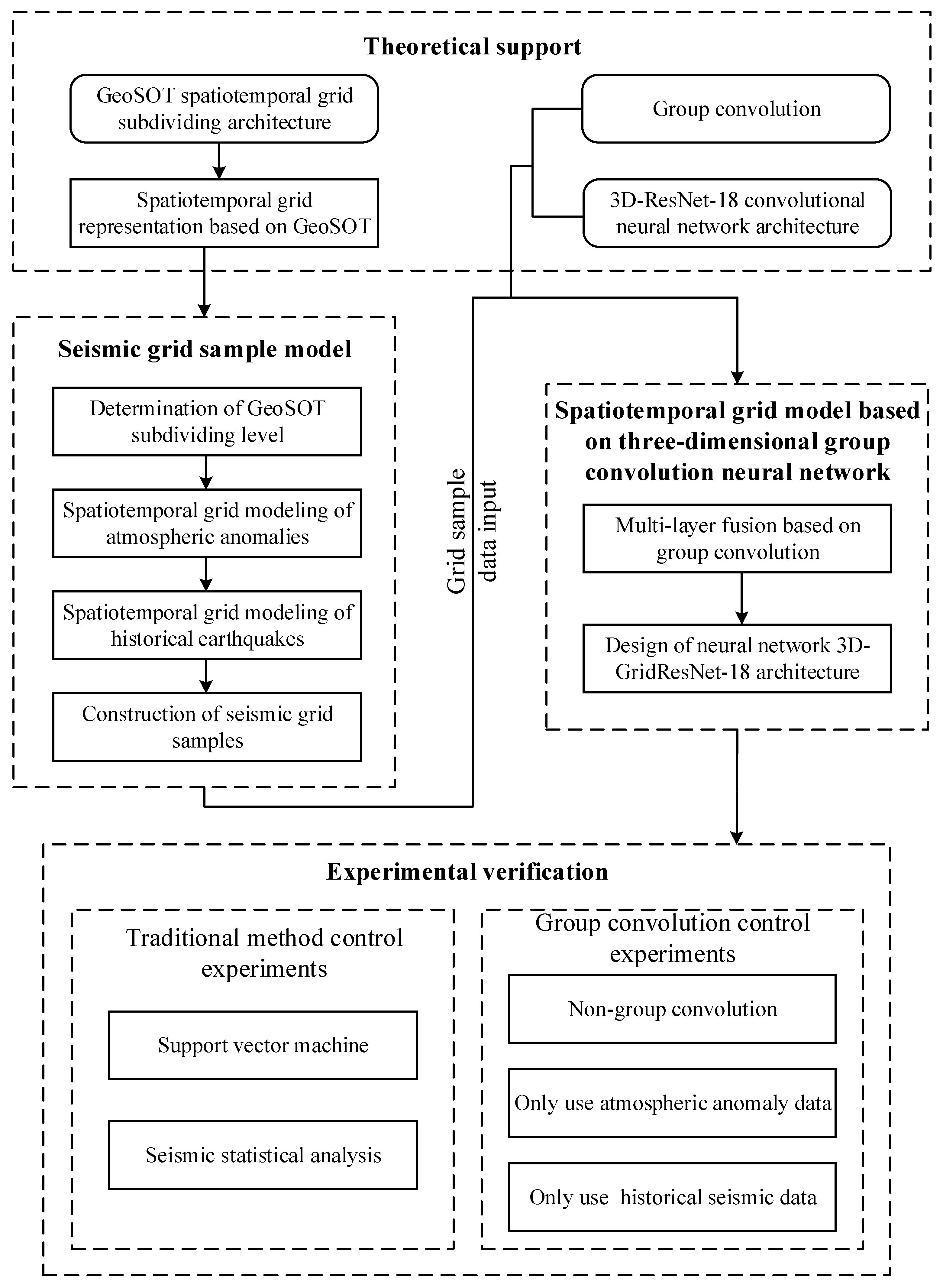
In summary, this study focuses on the deep learning of multiple spatial information in spatiotemporal big data, as shown in Figure 1. For earthquake warnings, this study proposes a seismic grid sample model (SGSM) organizing multiple single-layer data slice spatial information data to form a multi-layer data block with a consistent data structure oriented to the deep learning model. Furthermore, the study proposes a spatiotemporal grid model based on a three-dimensional group convolution neural network (3DGCNN-SGM) to improve the learning effect of the integration analysis of multiple spatial information.

2. Materials and Methods

2.1. Spatiotemporal Grid Representation Based on GeoSOT

The geographical coordinate grid subdivision by a one-dimensional integer and two-to-nth power (GeoSOT) [32] is a global equal longitude and latitude spherical subdividing grid system proposed by Cheng’s team at Peking University. This system has the advantages of multi-scale, identifiable, localizable, indexable, computable, and automatic spatial association, constituting a spatial grid framework for big data management and application. The GeoSOT grid extends the latitude and longitude space of the Earth’s surface three times and then divides the whole Earth into a hierarchical grid system of the integer degree, integer minute, integer second, and below from global to centimeter by a strict recursive quadtree partition. Specifically, the first space expansion is to expand the whole Earth’s surface to 512° × 512°; the center of the patch coincides with the intersection of the equator and the prime meridian, and then recursively quads to a 1° grid unit. The second space expansion is purposed to expand the 1° grid unit from 60’ to 64’ and then recursively quad to one grid unit. The third space expansion is purposed to expand the 1’ grid unit from 60” to 64” and then recursively quad to 1” grid unit. The subdivision units below 1” are directly divided by a quadtree partition until (1/2048)” of 32 levels. In this way, GeoSOT divides the longitude and latitude space of the whole Earth surface into a multi-level grid system covering the whole world in the direction of longitude and latitude through a strict dichotomy.

The difficulty with spatiotemporal object modeling concerns extending the spatial grid to express the temporal changes in spatial objects. Space and time are typically considered as two mutually orthogonal dimensions and therefore the current idea of spatiotemporal object modeling is to add an additional model dimension to the spatial object to represent time. This idea corresponds to the grid model, which expands the original two-dimensional spatial grid description to three dimensions. In the original two spatial dimensions, the spatial grid is used to model the spatial object at a specific time, whereas in the time dimension, the spatial data at different times are organized according to the time sequence and a certain time interval. In other words, the gridding description of spatiotemporal objects is essentially a three-dimensional grid set. The GeoSOT divides the Earth’s surface space into multilevel discrete regions with similar areas and shapes, with no gaps and no overlaps. Each discrete region is a spatial grid and the set of spatial grids can describe the spatial objects occupying the corresponding positions. Spatial objects continuously changing over time can be described by a set of spatial grids for each specific time. Then, the spatial grid sets are organized according to the time sequence and specific time interval to form the grid description of the spatial objects. Thus, a single spatiotemporal grid constitutes the basic description unit of the GeoSOT subdividing data model for spatiotemporal objects.

Let the grid system of space subdivision be $ℂ=\left\{C_0,C_1,\dots C_i,\dots C_n\right\}$, where $C_i=C_{i0},C_{i1},\dots C_{ij},\dots C_{i{n}_i}$ represent all grids of the i-th level, and for any two grids of the i-th level, $C_{is},C_{it}\left(s\ne t\right)$, all $C_{is}\cap C_{it}=\varphi$. Then, for the spatial object $O$, let $O\left(Obj\right)$ denote the real space it occupies, $Ob{j}^{t_j}$ denote the space state of the object at the t_j moment, and the corresponding subdivision level of the representation accuracy of the spatial object at any time in the spatial grid system is r, where t_j = t₀,…,t_T. If the time difference between any two adjacent times ($\mathsf{\Delta }t$) is the same, the spatiotemporal object can be expressed as n_r sets of r-level spatiotemporal grids:

$$\{\begin{array}{c}G\left(Obj;r, \Delta t\right)=\underset{j=0}{\overset{T}{{\displaystyle \cup }}}{G}^{t_j}\left(Obj;r\right)=\underset{j=0}{\overset{T}{{\displaystyle \cup }}}\underset{C_{ri}\cap O\left(Obj\right)\ne \varnothing }{\overset{i\le n_r}{{\displaystyle \cup }}}{C}_{ri}^{t_j}\\ Attr\left(Obj;r,\Delta t\right)=\underset{j=0}{\overset{T}{{\displaystyle \cup }}}Att{r}^{t_j}\left(Obj;r\right)=\underset{j=0}{\overset{T}{{\displaystyle \cup }}}\underset{C_{ri}\cap O\left(Obj\right)\ne \varnothing }{\overset{i\le n_r}{{\displaystyle \cup }}}Attr\left(C_{ri}^{t_j}\right)\end{array}$$

(1)

2.2. SGSM

This study takes the seismic precursor data, atmospheric anomaly, to elaborate on the spatiotemporal grid modeling method. The aim of establishing the spatiotemporal grid model of atmospheric anomaly data is to determine the subdividing level of GeoSOT, establish the spatial interpolation model, and finally establish the spatiotemporal grid model of atmospheric anomaly data as a data composition type of SGSM.

2.2.1. Determination of GeoSOT Subdividing Level

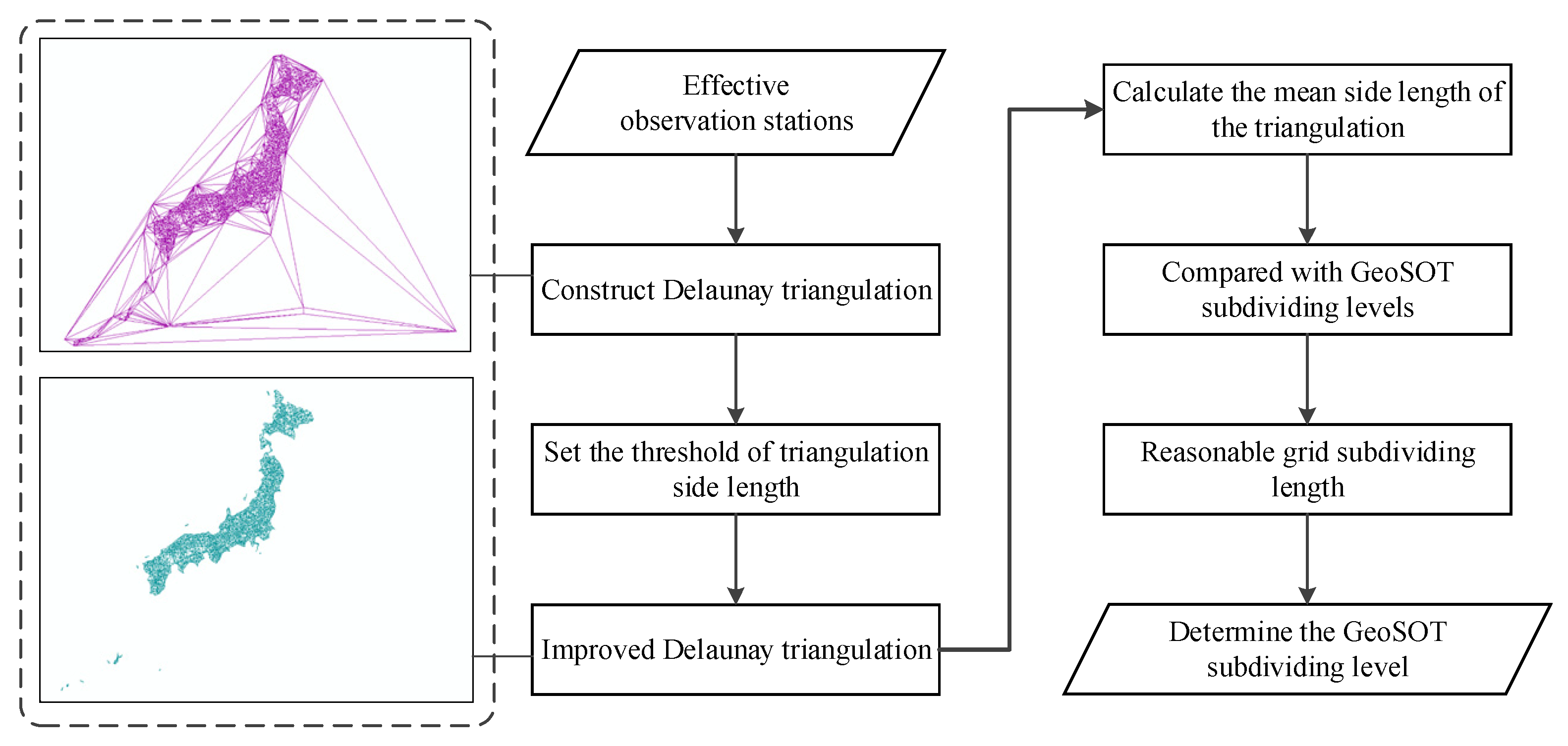
When establishing the spatial grid model of atmospheric anomaly data, according to the spatial distribution of meteorological stations (i.e., the spatial location information of atmospheric anomaly data), the appropriate analysis scale to determine the GeoSOT grid level is chosen. This paper proposes the use of Delaunay triangulation (DT) [33] to model the meteorological stations’ spatial distribution. The DT input is the discrete point of all meteorological station locations and the output is a series of connected triangles. All the triangle vertices correspond to all the meteorological station locations individually. The DT reflects the spatial distribution relationship between meteorological stations and the side length of the triangle reflects the relative distance between meteorological stations.

Based on DT, this study uses the average side length of DT as a measure of the distance between discrete atmospheric observation data, selects the grid level closest to the average side length of DT as the grid basis of the atmospheric anomaly data spatial grid model, and performs preliminary grid modeling of the atmospheric observation data. The determination process of the GeoSOT subdividing level of the seismic sample grid is shown in Figure 2.

2.2.2. Spatial Interpolation Model

Before spatial interpolation, this study takes air temperature data from atmospheric observation data of meteorological stations as an example to preprocess and obtain atmospheric anomaly data. This paper follows the definition of atmospheric temperature anomaly by Professor Murai’s team at the University of Tokyo [34]; that is, if the temperature changes by more than ±2 °C in 10 min at the same station, it is recorded as an anomaly. The total number of anomalies per day at each station was counted and the integer value was the atmospheric anomaly value of the station on that day.

In this study, the spatial interpolation of atmospheric anomalies after gridding is proposed to convert the measured data of discrete points into a continuous data surface so that the sparse and discrete atmospheric observation data can reflect the continuous atmospheric conditions. In many spatial interpolation algorithms, the inverse distance weight (IDW) [35] is a simple and general spatial interpolation algorithm. The IDW calculates the atmospheric anomalies on the non-data points using the weighted average of each atmospheric anomaly observation value in the adjacent area and the weight of each observation value decreases with an increase in the distance between the observation and the prediction point. Specifically, let x₀ represent the position of the point to be interpolated, while u₀ represents the interpolation result to be calculated, ${\left\{x_i\right\}}_{i=1}^N$ denotes the positions of N known atmospheric anomaly observation points, and ${\left\{u_i\right\}}_{i=1}^N$ are known atmospheric anomaly values.

$$u_0=\frac{{\sum }_{i=1}^{N}w\left(x_0,x_i\right)u_i}{{\sum }_{i=1}^{N}w\left(x_0,x_i\right)}$$

(2)

$$w\left(x_0,x_i\right)=\frac{1}{d{\left(x_0,x_i\right)}^p}$$

(3)

where d(x₀,x_i) denotes the distance between x₀ and x_i, and p is the super parameter of the model to adjust the weight. Based on IDW, Formulas (2) and (3), the atmospheric anomaly values of all spatial grids after gridding, can be calculated to establish the spatial grid model of atmospheric anomaly data.

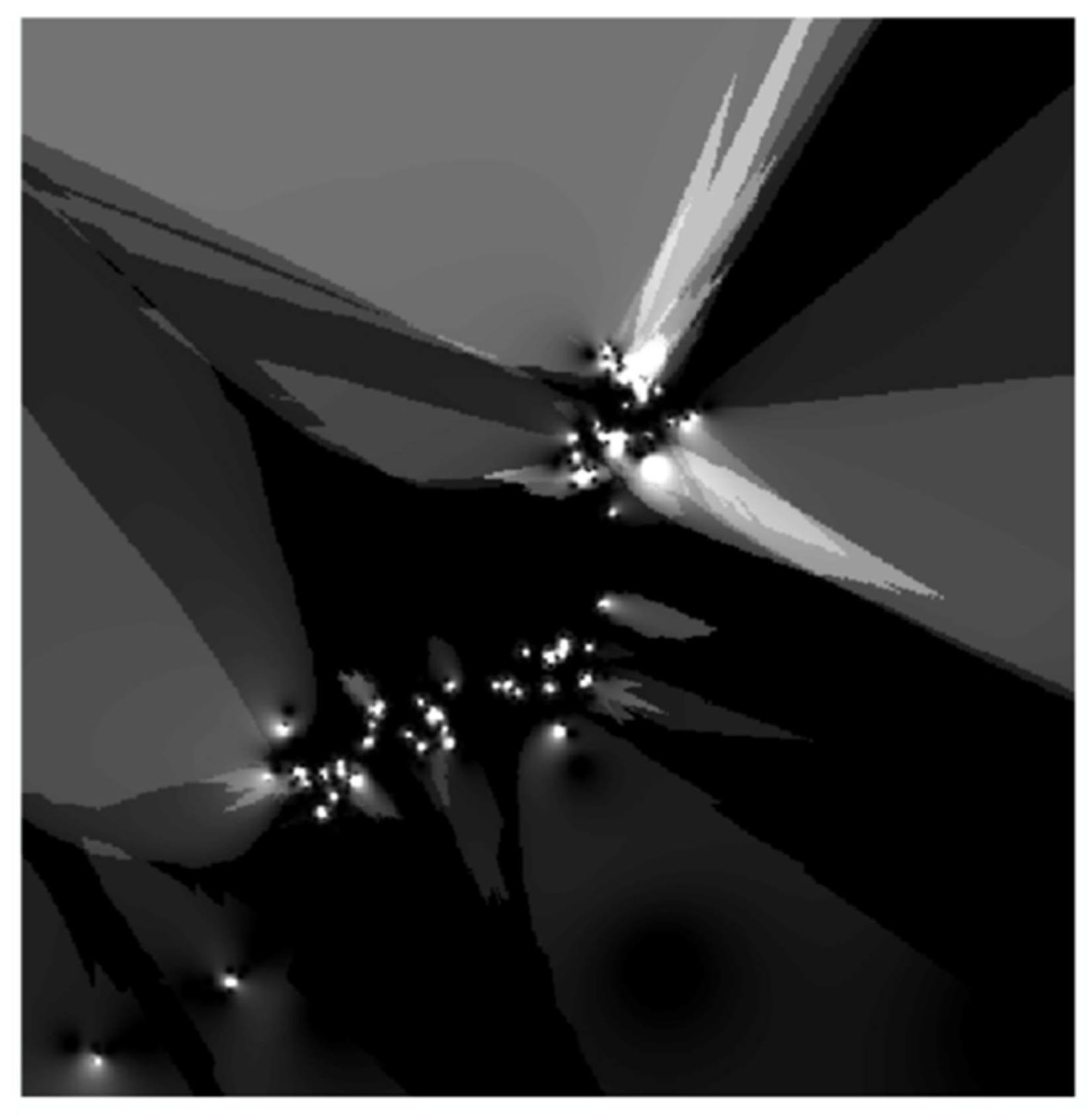
Based on the spatial grid model of atmospheric anomaly data, according to the time scale of atmospheric observation data, the appropriate time interval was determined to establish the spatiotemporal grid model of atmospheric anomaly data. Specifically, for each time, a space grid of $H\ast W$ was used to model the atmospheric anomaly data at that time, as shown in Figure 3. If the total time span of all data is T and the established time interval is Δt, then there are $C=T/\mathsf{\Delta }t$ $H\ast W$ spatial grids; that is, the spatiotemporal grid model of atmospheric anomaly data is a three-dimensional spatiotemporal grid of $H\ast W\ast C$.

2.2.3. Spatiotemporal Grid Modeling and Grid Sample Construction of Seismic Precursor Data

The result of the spatiotemporal grid modeling of atmospheric anomalies is the data matrix $G\left(A;r,\Delta t\right)={{\displaystyle \cup }}_{j=0}^T{G}^{t_j}\left(A;r\right)\to X\left(A\right)\in R^{C\ast H\ast W}$ (A is used to represent the atmospheric anomaly). In this study, historical seismic data were modeled based on the spatiotemporal grid of atmospheric anomalies. E was used to represent historical seismic data, the attribute value of each grid was the seismic intensity value, and the modeling result of historical seismic data was $G\left(E;r,\Delta t\right)={{\displaystyle \cup }}_{j=0}^T{G}^{t_j}\left(E;r\right)\to X\left(E\right)\in R^{C\ast H\ast W}$. The seismic spatiotemporal grid modeling result is $X\left(m\right)=\left\{X\left(A\right), X\left(E\right), \dots \right\}$ (m is the number of data types).

If we set the space window size of samples as ws and the time window size as Δts, the size of each grid sample is $x\left(m\right)\in R^{m\ast \Delta ts\ast ws\ast ws}$. In this study, the method of sample labeling is to calculate the maximum seismic intensity value of the last day in the grid of $\Delta ts\ast ws\ast ws$, denoted as M. It is considered that the atmospheric anomaly of the grid sample is associated with the maximum earthquake, that is, y₁ = M, and forms a binary {x,y₁}. The sample with an earthquake is the positive grid sample (PGS), while the sample without an earthquake is a negative grid sample (NGS), that is, y₀ = 0, and PGS also forms a binary {x,y₀}. Then, SGSM is $\{\begin{array}{c} \left\{x,y_0\right\}, y_0=0 \\ \left\{x,y_1\right\}, y_1=M\end{array}$.

This study uses a method of grid sample extraction based on the sliding window; that is, starting from the top left of the spatiotemporal grid, every time a grid sample is taken out according to the window, it moves one step S to the right and then the next grid sample is taken out. When moving to the far right of the current row, return to the far left, and move one step S down to repeat the above process. The sliding step size S is consistent with the size of the spatiotemporal grid, which minimizes the redundancy in the data and improves the utilization of all data.

2.3. Spatiotemporal Grid Model Based on the Three-Dimensional Group Convolution Neural Network (3DGCNN-SGM)

2.3.1. Multi-Layer Fusion Based on Group Convolution

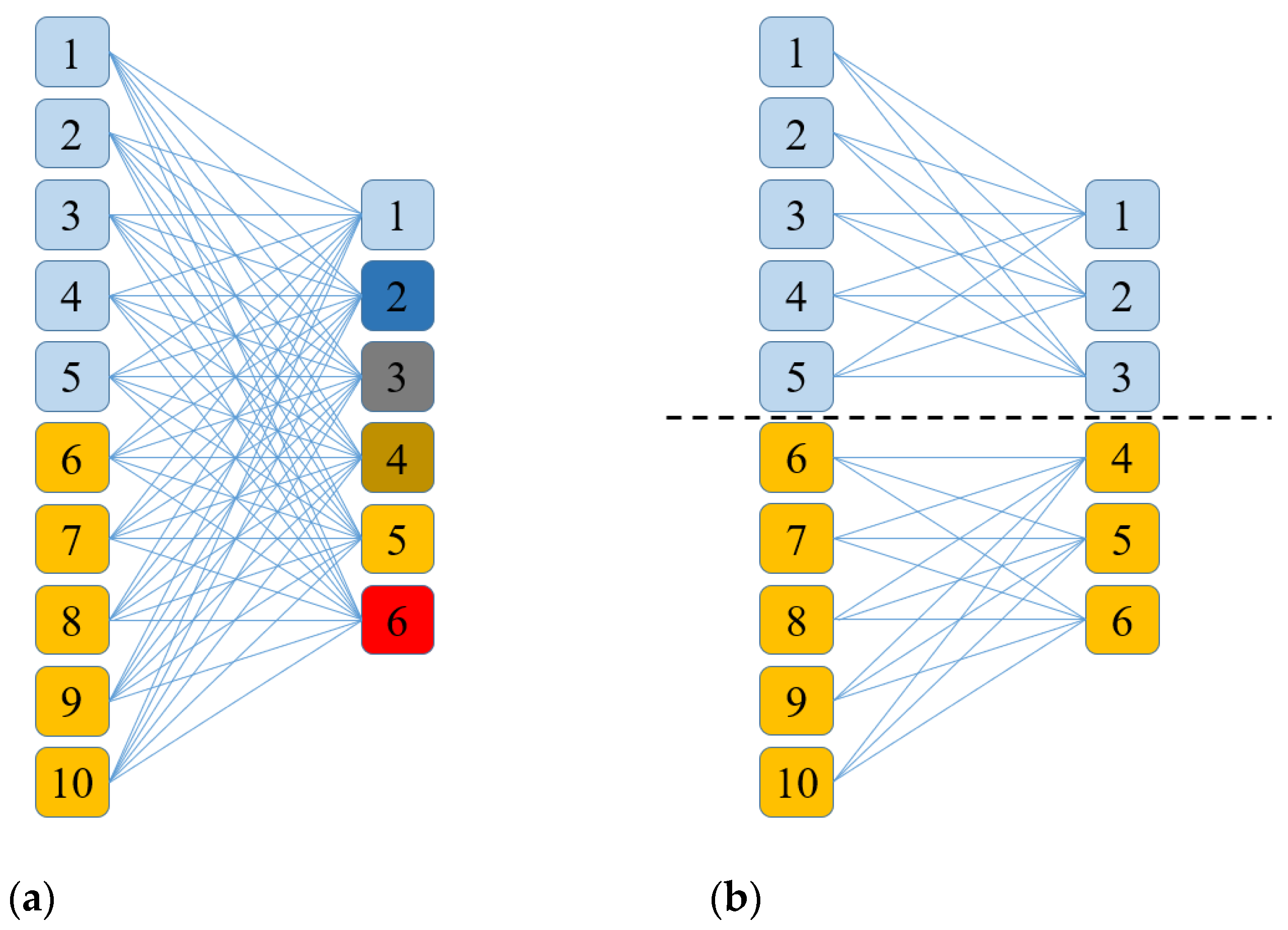
When feature maps come from different layers, they lack direct comparability, which confuses the features of different layers and then affects the neural network’s representation ability and classification results. Group convolution is an algorithm for grouping and stacking different characteristic graphs, which provides a new neural network architecture design for multi-source data fusion [36].

For the original total number of C input characteristic graphs, the group convolution divides these characteristic graphs into g groups; that is, each group has $C/g$ characteristic graphs and the superposition of convolution results is only carried out within the group. Let $a_q^l$ be the q-th characteristic graph of layer l and $K_p^l$ be the p-th convolution kernel of layer l. The input and output characteristic graphs are multiple three-dimensional matrices (i.e., the set of these characteristic graphs is four-dimensional) and the convolution kernel is also several three-dimensional matrices. The calculation formula for the group convolution is as follows:

$$a_p^l\left(i,j,t\right)=\sigma \left({\displaystyle \sum }_{q=1}^{C/g}{\displaystyle \sum }_u{\displaystyle \sum }_v{\displaystyle \sum }_w{a}_q^{l-1}\left(u,v,w\right)K_p^l\left(i-u,j-v,t-w\right)\right)$$

(4)

where, in $a_p^l\left(i,j,t\right)$, representing the element on the i-th row and j-th column of the characteristic graph a, t is the time dimension and $\forall p, l, K_p^l\in \theta$.

A schematic of the group convolution principle is shown in Figure 4b.

2.3.2. Architecture of 3DGCNN-SGM: 3D-GridResNet-18

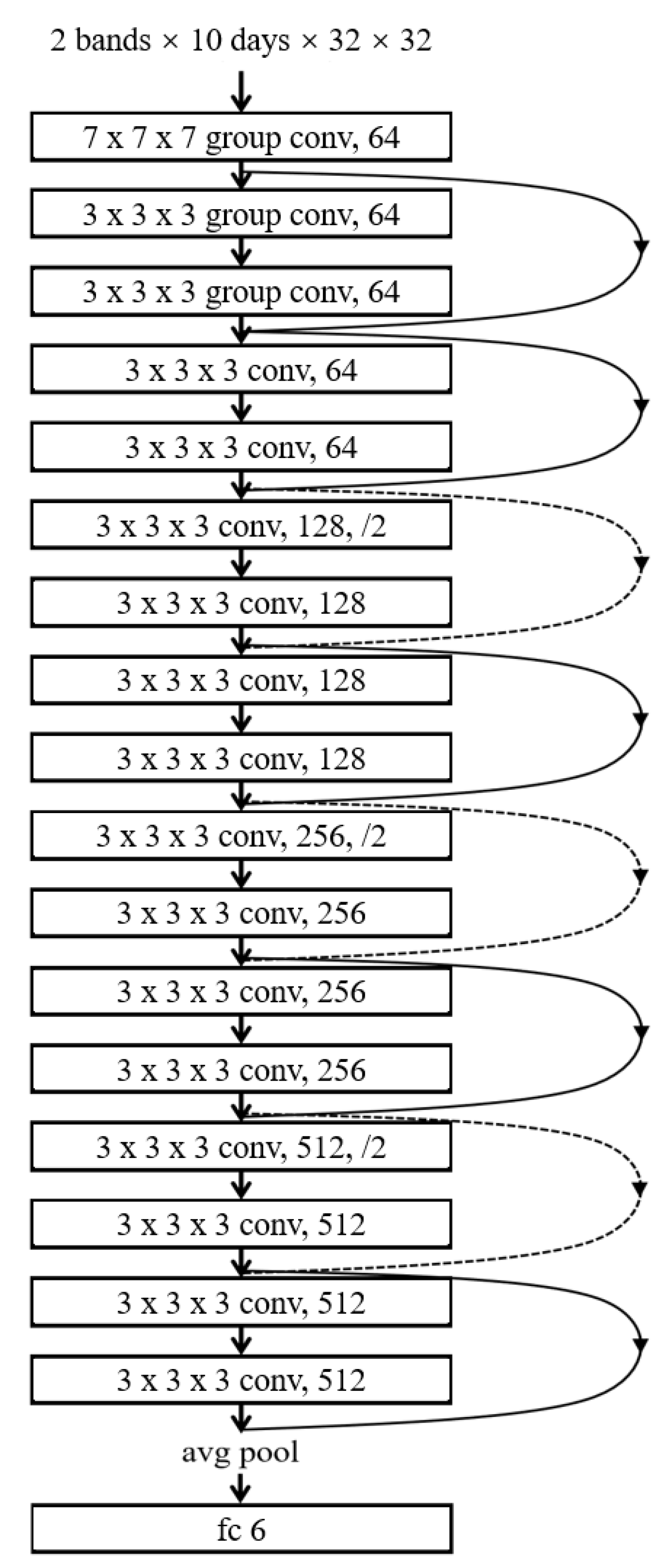
When an earthquake is expressed as a point object described by a single spatiotemporal grid, the corresponding problem form for establishing the association between seismic precursory data and earthquakes is a classification problem in deep learning. Its input is SGSM and its output is the prediction of whether the central grid of the SGSM is the epicenter of the earthquake. To establish the spatiotemporal association, that is, to solve the above classification problem, this study proposes a deep CNN algorithm model, 3D-GridResNet-18, based on SGSM and 3D-ResNet-18 [37]. The network architecture of 3D-GridResNet-18 is shown in Figure 5.

The special structure of 3D-ResNet-18 is the residual learning unit. In a residual learning unit, a neural network is divided into two branches. Let the input characteristic graph of this unit be a^l−1 and then its output is

$$a^l=F\left(Z^l;a^{l-1}\right)+a^{l-1}$$

(5)

In Equation (5), the first term $F\left(Z^l;a^{l-1}\right)$ represents the original backbone of the neural network, that is, the building block of the convolution layer-batch normalization (BN) layer-activation layer and Z^l represents the model parameters of 3D-ResNet-18. The second term a^l−1 indicates that the original input has an identity mapping; that is, the input data does not participate in the operation of the backbone network but is directly added to the operation result of the building block. The residual learning unit enables 3D-ResNet-18 to learn new features based on the original input features. In the worst case, it does not learn any new features but only uses the input to create the output directly. This structure makes it easier for the deep CNN to complete training and produces better performance. Corresponding to Figure 5, each arc on the side of the network backbone corresponds to identity mapping. The result of identity mapping is typically added before the activation layer of the building block; that is, the structure of the building block pointed by the arced arrow becomes a convolution layer-BN layer-join identity mapping-activation layer. If the building block has a pooling layer, the pooling layer is connected after the activation layer.

Based on 3D-ResNet-18, the corresponding improvements were made to form 3D-GridResNet-18 for SGSM. First, the experimental data included both the atmospheric anomaly data and the historical earthquake data, forming two channels. Therefore, the convolution kernel of the first convolution layer of 3D-ResNet-18 was changed to 2 × 7 × 7 × 7 so that it could process SGSM. In addition, the seismic intensity levels involved in this experiment were 0, 2–6, and a total of six levels; that is, 3D-GridResNet-18 deals with a six-classification problem. Therefore, the last output layer of 3D-ResNet-18 is modified to have six output units to predict the probability of earthquakes of any intensity. Finally, in the first three layers of 3D-ResNet-18, we used group convolution instead of ordinary convolution.

Each rectangular box in 3D-GridResNet-18 represents a building block comprising a convolution layer, a BN layer, and an activation layer. For all the convolution layers in 3D-GridResNet-18, the strategy of padding is to fill one 0 at each end of the two dimensions of the feature graph, that is, padding = (1,1). In addition, none of the convolution layers used the bias term. These parameters are in line with the default parameters of the ResNet-18 framework provided by Pytorch. The total number of model parameters for 3D-GridResNet-18 was 33052999.

2.4. Experiment

2.4.1. Experimental Data and Environment

The experiment validates the SGMG-EEW. To verify the effectiveness of the proposed SGSM and 3DGCNN-SGM, five groups of control experiments were designed: a group using atmospheric anomaly data (AA-C) only; a group using historical earthquake data (HE-C) only; a non-group convolution control group (NG-C); a SVM control group (SVM-C); and a seismic statistical analysis control group (SSA-C).

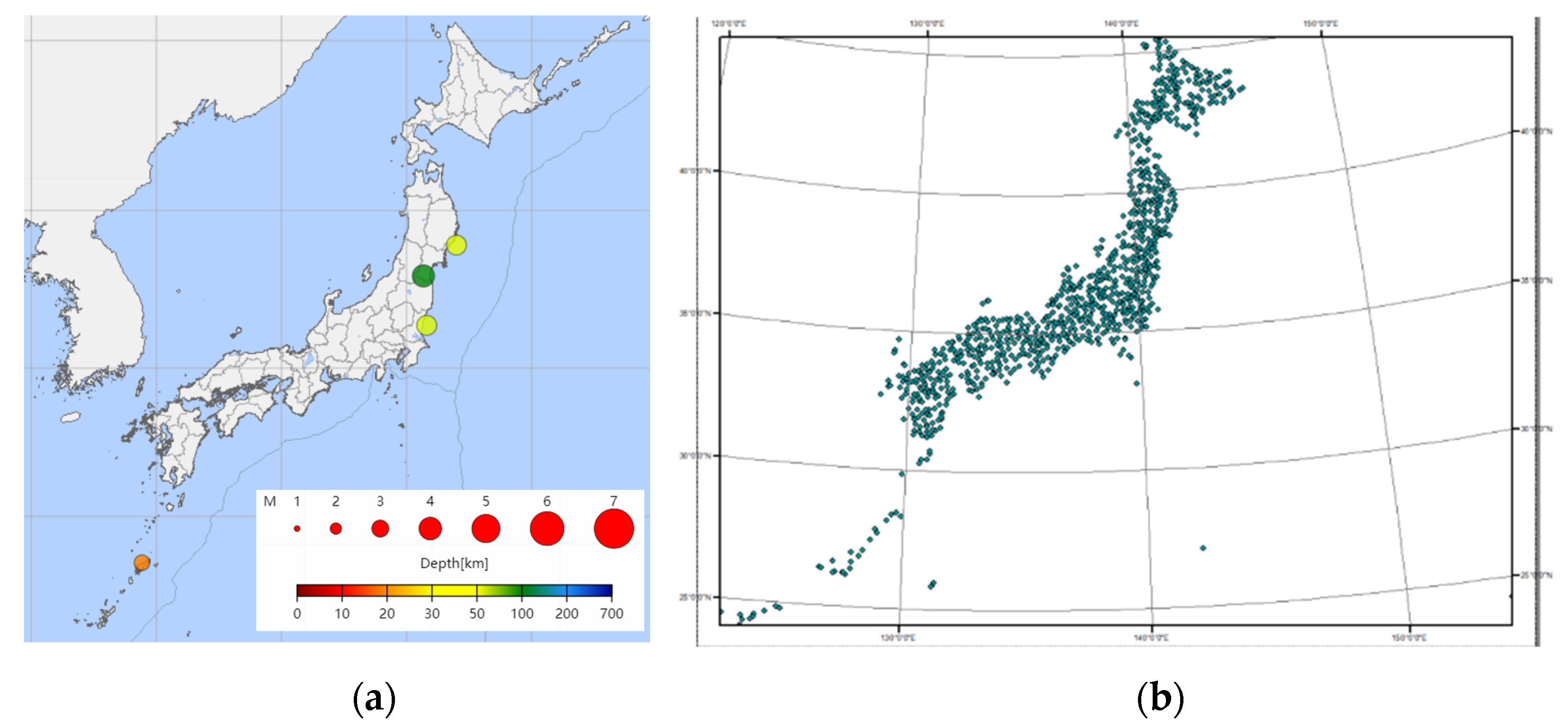
The data used in this experiment are atmospheric data and seismic data, the space span of which is all of Japan and the time span is from 1 June 2018 to 31 December 2019, a total of 19 months. The details of the data are presented in

Table 1. Detailed information on atmospheric data and seismic data.

Data Type	Recording Time	Recording Frequency	Number of Stations	Recording Accuracy	Data Content	Number of Records
Seismic data	1 June 2018–31 December 2019	NULL	NULL	0.1	The time of the earthquake, longitude and latitude of the epicenter, earthquake intensity, maximum earthquake intensity, etc.	1207
Atmospheric data		Time interval: 10 min	967 (valid)	0.1	Temperature, air pressure, precipitation, relative humidity, sunshine time, etc.	80,624,592

; the source of the seismic data is the epicenter data released by the Japan Meteorological Agency and a schematic of the true seismic values is shown in Figure 6a. Atmospheric data are the atmospheric observation results of various meteorological stations in Japan. The spatial distribution of the meteorological stations is shown in Figure 6b.

According to Section 2.2.1, the 13th level, the 4’ subdividing grid of GeoSOT, is selected in this experiment and the plane distance of its side length is 8 km. Each unknown point in the spatial interpolation model (Section 2.2.2) uses the data of 12 known points around and the form of the distance weight is set as the inverse square weight; that is, p = 2 in Equation (3). The SGSM parameters are set to $m=2, \Delta ts=10, ws=32, \mathsf{\Delta }t=1, T=546, H=444, \mathrm{and} W=433, S=32$. Some PGS and NGS, the data input of the deep learning analysis models, were extracted. For PGS, this experiment used a 7:3 training test data partition ratio. The distribution of the grid samples is presented in

Table 2. Distribution of grid samples.

	PGS	NGS	Total
Training data	837	9000	9837
Test data	370	450	820

.

2.4.2. Experimental Results and Analysis

Accuracy, precision, recall, and the F₁-Measure evaluation methods were adopted. The calculation formulas are defined as follows:

$$Acc=\frac{TP+TN}{TP+TN+FP+FN}\times 100\%,$$

(6)

$$P=\frac{TP}{TP+FP}\times 100\%,$$

(7)

$$R=\frac{TP}{TP+FN}\times 100\%, \mathrm{and}$$

(8)

$$F_1=\frac{2\ast P\ast R}{P+R},$$

(9)

where $Acc$ is the accuracy, P is the precision, R is the recall, TP is the number of correctly predicting positive classes to the positive classes, TN is the number of correctly predicting negative classes to negative classes, FP is the number of mis-predicting negative classes to positive classes, and FN is the number of mis-predicting positive classes to negative classes.

For regression problems, the mean square error (MSE) is typically used to measure the difference between the predicted and real values. The smaller the value of MSE, the closer the prediction is to the real value and the better the performance of the model. Its specific definition is as follows:

$$MSE=\frac{1}{N}{\displaystyle \sum }_{i=1}^N{\left(\widehat{y_i}-y_i\right)}^2$$

(10)

where y_i is the real value, $\widehat{y_i}$ is the predicted value, and N is the number of predictions.

3. Results

3.1. SGMG-EEW Training and Test Results

The SGMG-EEW model parameter initialization adopts the fine-tune method based on 3D-ResNet-18. For the part in which the network architecture is consistent with 3D-ResNet-18, the initial parameter values are set to the model parameters of Hara et al [38] who pretrained 3D-ResNet-18. For the part of the network architecture inconsistent with 3D-ResNet-18, including the first convolution layer and the last fully connected layer, the parameter initialization method uses the Pytorch default normal distribution initialization based on the number of parameters. For the training algorithm Adam, this experiment sets its initial learning rate to 0.001 and the parameters of the Adam algorithm, namely β₁ and β₂, use the recommended value of the algorithm proposer, that is, β₁ = 0.9, β₂ = 0.999. The number of iterations was 80 and the batch size was set to 64. In this experiment, the cross-entropy loss function was selected as the model strategy. The cross-entropy loss function is a common loss function in deep learning classification. The concrete form is as follows:

$$L\left(\widehat{y_i^c},y_i^c\right)=-{\displaystyle \sum }_{c=1}^{N_c}{y}_i^c\log \left(\widehat{y_i^c}\right)$$

(11)

where c is the real class of the sample and N_c is the total number of real classes. $y_i^c$ indicates whether the label of the ith sample is class C (if yes, then $y_i^c=1$; otherwise $y_i^c=0$). $\widehat{y_i^c}$ denotes the model judgment of the probability that sample x_i is class C. In this experiment, there were six earthquake intensity levels; that is, there were six classification problems and N_c = 6.

To test the reliability of the results, different random seeds are used to establish the dataset, divide the training-test data set, initialize the model parameters, and estimate the model parameters. Ten experiments were repeated. Each experiment recorded the loss function curve on the training set, the confusion matrix of intensity estimation on the test set, the average precision, the MSE and the confusion matrix of the position estimation on the test set and calculated their mean values and the variances of the evaluation indexes.

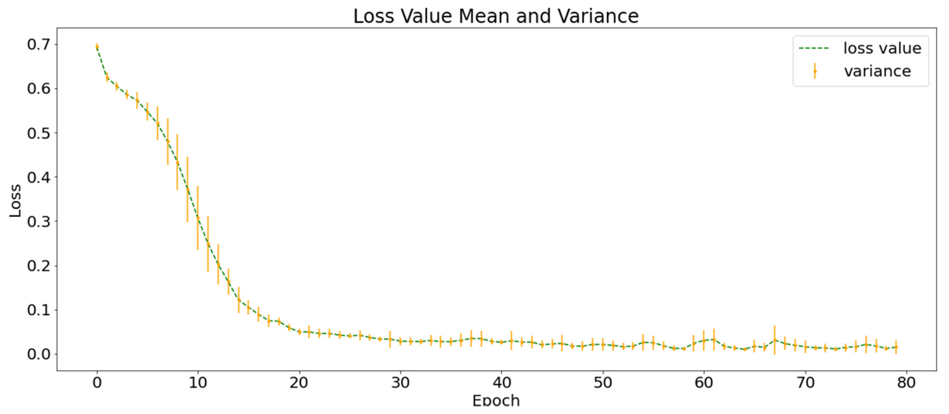
Figure 7 shows the average loss function curves of the ten training processes. The green dotted line represents the mean value of the loss function in the ten experiments and the orange vertical line represents the variance of the loss function value at this point. At the end of the training, the value of the loss function converges to approximately 0.02 and the $Acc$ of the training set classification in the ten experiments was higher than 99%.

Table 3. Confusion matrix of the seismic intensity classification on the test set.

Intensity	0	2	3	4	5	6
0	386.5 ± 8.6	3.2 ± 1.5	7.1 ± 2.8	6.9 ± 2.6	0.7 ± 0.9	0.4 ± 0.9
2	17.4 ± 5.0	56.0 ± 4.2	1.4 ± 1.2	0.5 ± 0.8	0.1 ± 0.3	0.1 ± 0.3
3	30.9 ± 6.1	1.1 ± 1.2	106.9 ± 9.3	3.2 ± 1.6	0.3 ± 0.6	0.0 ± 0.0
4	36.2 ± 4.7	0.4 ± 0.7	2.4 ± 1.1	123.0 ± 8.9	1.1 ± 1.4	0.0 ± 0.0
5	7.1 ± 2.7	0.0 ± 0.0	0.5 ± 0.7	0.4 ± 0.5	19.3 ± 2.8	0.0 ± 0.0
6	2.4 ± 1.4	0.0 ± 0.0	0.0 ± 0.0	0.1 ± 0.3	0.0 ± 0.0	4.4 ± 1.4

shows the mean and variance of the confusion matrices of the models trained in the ten experiments on the test set, in which each row represents the actual intensity of the earthquake and each column represents the seismic intensity determined by the model. The first term of each cell is the mean of the ten predictions and the second term is the variance of the ten predictions. As shown in Table 3, there are two main types of errors in the prediction of seismic intensity: the first is predicting the actual earthquake samples as “no earthquake” and the second concerns that the predicted value is similar to the real value but somewhat different. Except for the no-earthquake class, there was little difference between the predicted value and actual value.

Based on the confusion matrix, P, R, and F₁ for each class can be calculated. The values and their variances are presented in

Table 4. Results of the seismic intensity classification evaluation indices on the test set.

Intensity	0	2	3	4	5	6
P	0.80 ± 0.02	0.92 ± 0.04	0.91 ± 0.02	0.92 ± 0.03	0.91 ± 0.10	0.92 ± 0.19
R	0.95 ± 0.01	0.74 ± 0.05	0.75 ± 0.05	0.75 ± 0.02	0.71 ± 0.09	0.65 ± 0.10
F1	0.87 ± 0.01	0.82 ± 0.04	0.82 ± 0.03	0.83 ± 0.02	0.79 ± 0.06	0.75 ± 0.13

. The results show that the precision of earthquake prediction is high but the recall is low. This is because, in many cases, the samples with earthquakes are predicted to have no earthquakes, which is consistent with the results of the confusion matrix.

The average $Acc$ of the then experiments on the test set was 84.89 ± 1.76% and MSE was 1.74 ± 0.20. The result of MSE is consistent with the result of the confusion matrix in Table 3; that is, the model can easily predict the earthquake to the adjacent 1–2 magnitude range of real intensity.

The prediction results of earthquake intensity also included the prediction results of the earthquake location. Therefore, based on the classification prediction of earthquake intensity, the prediction results are divided into earthquake and no earthquake, the 1–6 levels in the intensity classification are merged into an earthquake, and the classification prediction of the earthquake location can be obtained.

Table 5. Confusion matrix of the earthquake location classification on the test set.

	No Earthquake	Earthquake
No earthquake	386.5 ± 8.65	18.3 ± 4.86
Earthquake	94.0 ± 13.21	321.2 ± 10.00

shows the confusion matrix of earthquake location prediction in the ten experiments, in which each row represents whether there is an earthquake and each column represents the model’s prediction. The first term of each cell is the mean of the ten predictions and the second term is the variance of the ten predictions. From the confusion matrix, the overall $Acc$ of the earthquake location was 86.3%.

3.2. Control Group Using Atmospheric Anomaly Data Only

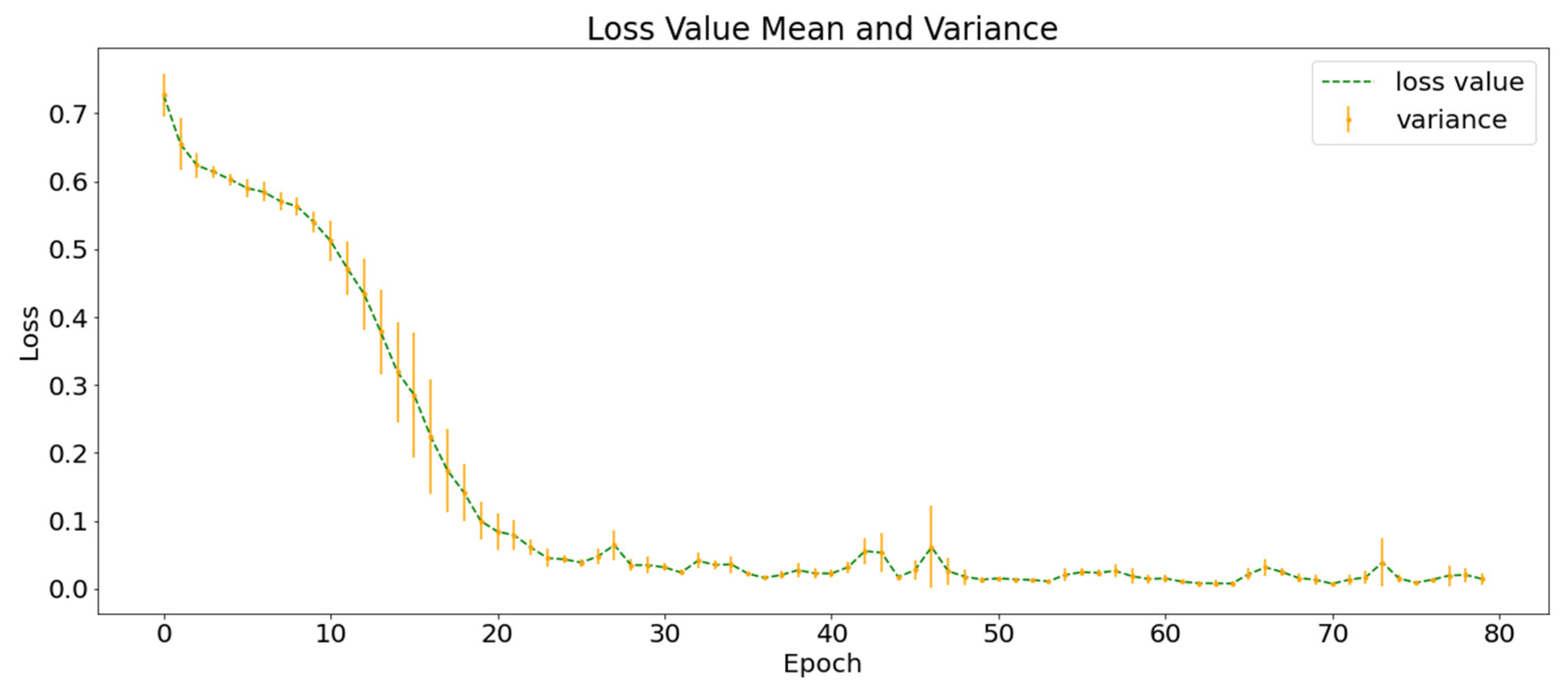
To explore the role of multi-layer information integration in earthquake prediction, this study designs a control experiment based on SGSM using only atmospheric anomaly data and uses a 3D neural network without group convolution for earthquake prediction. The AA-C was repeated three times with different random dataset partitions and neural network initial parameters. Figure 8 shows the mean and variance of the training loss function curves of AA-C. The shape of the curve is very similar to that of SGMG-EEW, the final loss function value also converges to approximately 0.02, and the $Acc$ of the training set is higher than 99%.

Table 6. Confusion matrix of the seismic intensity classification on the test set.

Intensity	0	2	3	4	5	6
0	387.3 ± 5.7	2.0 ± 0.8	6.7 ± 1.2	4.7 ± 1.7	0.0 ± 0.0	0.7 ± 0.5
2	20.0 ± 3.3	56.0 ± 6.5	2.0 ± 0.8	0.3 ± 0.5	0.3 ± 0.5	0.0 ± 0.0
3	29.3 ± 7.9	1.3 ± 1.2	105.7 ± 12.4	6.0 ± 0.8	0.0 ± 0.0	0.0 ± 0.0
4	40.3 ± 7.6	0.3 ± 0.5	1.0 ± 0.8	119.3 ± 7.0	1.0 ± 0.8	0.0 ± 0.0
5	8.0 ± 2.4	0.0 ± 0.0	0.0 ± 0.0	1.3 ± 0.9	19.7 ± 2.9	0.0 ± 0.0
6	1.7 ± 0.9	0.0 ± 0.0	0.0 ± 0.0	0.3 ± 0.5	0.0 ± 0.0	4.7 ± 1.7

shows the confusion matrix of the seismic intensity classification of AA-C on the test set. The results show that there are also some cases in AA-C in which some true values with earthquakes are predicted as no earthquakes.

Based on the confusion matrix, P, R, and F₁ for each class can be calculated. The index values and their variances are listed in

Table 7. Results of the seismic intensity classification evaluation indices on the test set.

Intensity	0	2	3	4	5	6
P	0.80 ± 0.03	0.94 ± 0.02	0.92 ± 0.01	0.90 ± 0.01	0.94 ± 0.05	0.85 ± 0.11
R	0.97 ± 0.01	0.71 ± 0.03	0.74 ± 0.07	0.74 ± 0.03	0.68 ± 0.10	0.73 ± 0.07
F1	0.87 ± 0.02	0.81 ± 0.03	0.82 ± 0.05	0.81 ± 0.01	0.78 ± 0.06	0.77 ± 0.02

. The overall $Acc$ of the three experiments was 84.47 ± 2.30% and MSE was 1.75 ± 0.24.

3.3. Control Group Using Historical Earthquake Data Only

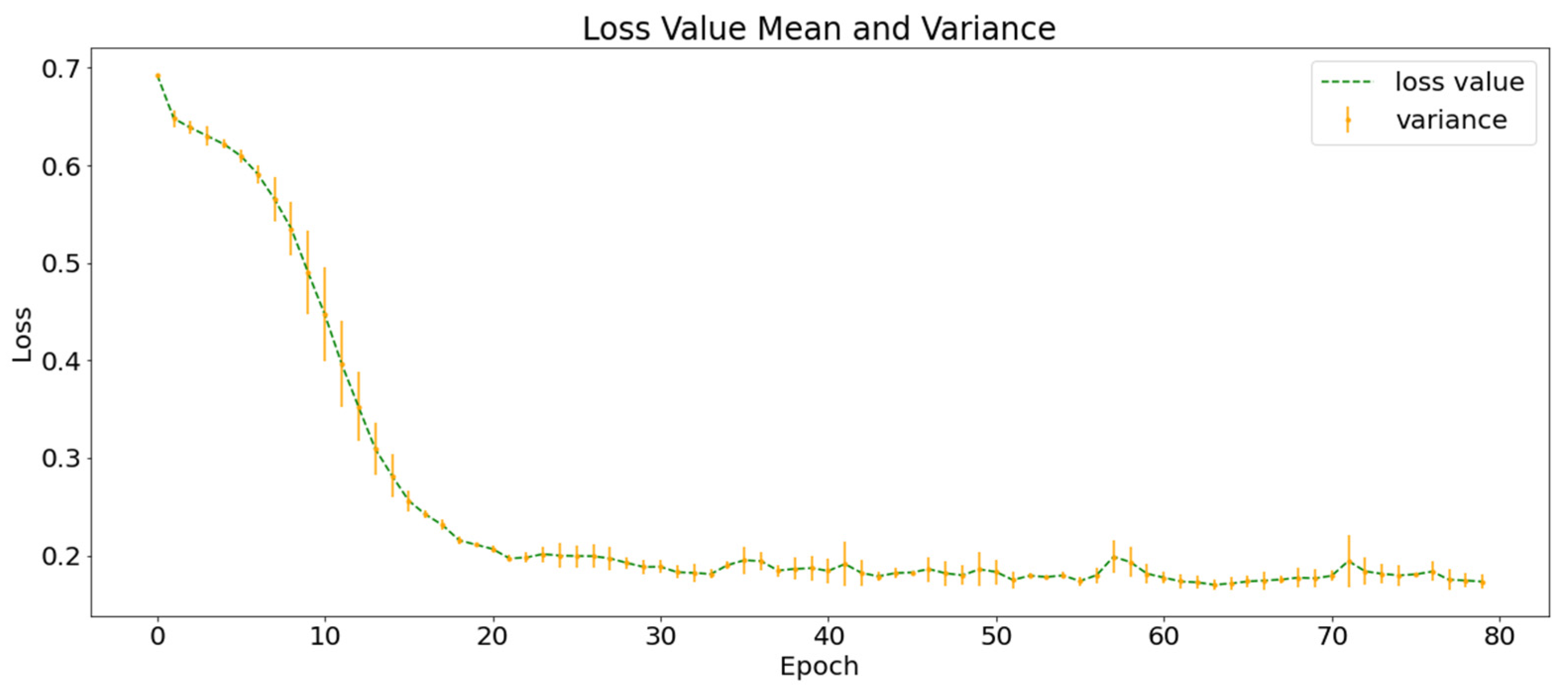
To further explore the role of multi-layer information integration in earthquake prediction, this study designed a control experiment based on SGSM using only historical earthquake data and used a 3D neural network without group convolution for earthquake prediction. The HE-C was repeated three times with different random dataset partitions and neural network initial parameters. Figure 9 shows the mean and variance of the training loss function curves of the HE-C. The shape of the curve is very similar to that of SGMG-EEW, the final loss function value also converges to approximately 0.02, and the $Acc$ of the training set is higher than 99%.

Table 8. Confusion matrix of the seismic intensity classification on the test set.

Intensity	0	2	3	4	5	6
0	394.3 ± 3.1	2.3 ± 0.9	4.0 ± 1.6	8.0 ± 0.8	0.7 ± 0.5	0.0 ± 0.0
2	30.7 ± 6.6	39.0 ± 6.4	1.3 ± 1.2	0.7 ± 0.5	0.0 ± 0.0	0.0 ± 0.0
3	40.3 ± 4.0	3.7 ± 0.5	90.7 ± 1.2	4.3 ± 2.9	0.0 ± 0.0	0.0 ± 0.0
4	50.3 ± 6.2	0.7 ± 0.5	3.0 ± 0.8	109.7 ± 12.5	1.7 ± 0.9	0.0 ± 0.0
5	10.3 ± 2.6	0.0 ± 0.0	0.3 ± 0.5	0.3 ± 0.5	16.0 ± 2.2	0.0 ± 0.0
6	4.0 ± 0.8	0.0 ± 0.0	0.0 ± 0.0	0.0 ± 0.0	0.0 ± 0.0	3.7 ± 1.2

shows the confusion matrix of the seismic intensity classification of HE-C on the test set. The results show that there are also some cases in HE-C in which some true values with earthquakes are predicted as no earthquakes.

Based on the confusion matrix, P, R, and F₁ for each class can be calculated. The index values and their variances are listed in

Table 9. Results of the seismic intensity classification evaluation indices on the test set.

Intensity	0	2	3	4	5	6
P	0.74 ± 0.03	0.85 ± 0.02	0.91 ± 0.02	0.89 ± 0.01	0.87 ± 0.02	1.00 ± 0.00
R	0.96 ± 0.00	0.54 ± 0.07	0.65 ± 0.01	0.66 ± 0.05	0.60 ± 0.04	0.47 ± 0.13
F1	0.84 ± 0.02	0.66 ± 0.06	0.76 ± 0.01	0.76 ± 0.03	0.71 ± 0.04	0.63 ± 0.13

. The overall $Acc$ of the three experiments on the test set was 79.67 ± 1.85% and MSE was 2.32 ± 0.23.

3.4. Non-Group Convolution Control Group

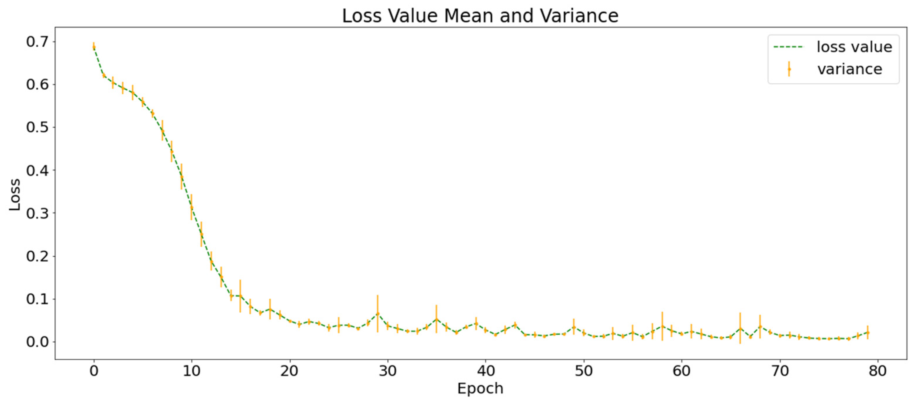
To verify the effect of group convolution in deep learning neural networks, this study designed a non-group convolution control experiment that used a 3D neural network without group convolution for the same training and test data. The group convolution used in 3D-GridResNet-18 was replaced by ordinary 3D convolution and the rest of the network structure was unchanged. The NG-C was repeated three times with different random dataset partitions and neural network initial parameters. Figure 10 shows the mean and variance of the training loss function curves of the NG-C. The shape of the curve is very similar to that of SGMG-EEW, the final loss function value also converges to approximately 0.02, and the $Acc$ of the training set is higher than 99%.

Table 10. Confusion matrix of the seismic intensity classification on the test set.

Intensity	0	2	3	4	5	6
0	386.0 ± 5.3	1. 7 ± 1.7	6.0 ± 0.8	6.3 ± 4.8	1.3 ± 1.9	0.0 ± 0.0
2	21.3 ± 3.4	55.3 ± 7.1	1.3 ± 0.5	0.7 ± 0.9	0.0 ± 0.0	0.0 ± 0.0
3	33.7 ± 8.2	1.7 ± 2.4	104.0 ± 13.1	2.7 ± 0.5	0.3 ± 0.5	0.0 ± 0.0
4	40.7 ± 10.2	0.7 ± 0.9	3.0 ± 0.8	117.0 ± 5.1	0.7 ± 0.9	0.0 ± 0.0
5	9.0 ± 2.9	0.0 ± 0.0	0.0 ± 0.0	0.3 ± 0.5	19.7 ± 2.9	0.0 ± 0.0
6	2.0 ± 1.4	0.0 ± 0.0	0.0 ± 0.0	0.0 ± 0.0	0.0 ± 0.0	4.7 ± 1.7

shows the confusion matrix of the seismic intensity classification of NG-C on the test set. The results show that there are also some cases in NG-C in which some true values with earthquakes are predicted as no earthquakes.

Based on the confusion matrix, P, R, and F₁ for each class can be calculated. The values of these indicators and their variances are presented in

Table 11. Results of the seismic intensity classification evaluation indices on the test set.

Intensity	0	2	3	4	5	6
P	0.78 ± 0.03	0.93 ± 0.07	0.91 ± 0.02	0.92 ± 0.05	0.89 ± 0.08	1.00 ± 0.00
R	0.96 ± 0.01	0.70 ± 0.04	0.73 ± 0.08	0.73 ± 0.04	0.68 ± 0.10	0.73 ± 0.07
F1	0.86 ± 0.02	0.80 ± 0.05	0.81 ± 0.06	0.81 ± 0.02	0.77 ± 0.06	0.84 ± 0.05

. The overall $Acc$ of the three experiments on the test set was 83.74 ± 1.76%, which is slightly lower than that of SGMG-EEW (84.89 ± 1.76%), and MSE is 1.89 ± 0.34, which is slightly higher than that of SGMG-EEW (1.74 ± 0.20). This shows that group convolution is beneficial for the deep learning of multi-layer data.

3.5. SVM Control Group

To verify the necessity of deep learning in earthquake warnings, the fourth control experiment in this study used the traditional statistical machine learning model. The data used were the atmospheric anomaly data and historical earthquake data from Japan, and the model used was the SVM [39].

The input data of SVM-C was a one-dimensional vector quantization of a 10 × 2 × 32 × 32 grid of each training sample of the atmospheric anomaly and historical earthquake data, and each training sample was a vector of 20,480 length. The division of the training and verification sets was consistent with the experimental group, and the maximum number of iterations of SVM-C training was set to 500.

Table 12. Confusion matrix of the seismic intensity classification on the test set.

Intensity	0	2	3	4	5	6
0	398	0	0	1	0	0
2	71	15	0	0	0	0
3	53	0	91	3	0	0
4	67	0	2	97	0	0
5	15	0	0	1	8	0
6	7	0	0	0	0	0

shows the confusion matrix of the seismic intensity classification of the SVM-C on the test set. The $Acc$ of SVM-C was significantly lower than that of deep learning methods. The results show that the correlation between seismic intensity and its precursor data is highly non-linear; thus, deep learning is necessary to establish this complex spatiotemporal correlation.

Based on the confusion matrix, P, R, and F₁ for each class can be calculated. These values are shown in

Table 13. Results of the seismic intensity classification evaluation indices on the test set.

Intensity	0	2	3	4	5	6
P	0.65	1.00	0.96	0.95	1.00	0.00
R	0.99	0.17	0.62	0.58	0.33	0.00
F1	0.78	0.30	0.75	0.72	0.50	0.00

, from which we can see that the problems of missing reports and low recall rates of earthquake warnings are more serious in a simpler model. The overall $Acc$ of the SVM-C on the test set was 72.99%.

3.6. Seismic Statistical Analysis Control Group

To verify the necessity of SGSM in earthquake warnings, the fifth control experiment in this study used the traditional seismic statistical analysis model. The atmospheric anomaly data and historical earthquake data from Japan were used, and the seismic statistical analysis method was the GR model. The SVM model was used to predict whether earthquakes would occur based on the stress characteristics extracted by the GR model. In the GR model, parameter b is considered to reflect the stress state of the crust and is an important parameter in seismic statistical analysis. Using the magnitude data within a certain time and space range, the maximum likelihood estimation formula for parameter b is as follows:

$$b=\frac{{\log }_{10}e}{\overline{M}-M_0}$$

(12)

where $\overline{M}$ is the mean magnitude of the seismic data used and M₀ is the threshold of the earthquake magnitude.

The SSA-C input data was a one-dimensional vector with a length of 20 generated by each 10 × 2 × 32 × 32 grid. The first ten features were b values calculated every day for 10 days and the last ten features were the average values of atmospheric anomalies. The division of the training and verification sets was consistent with the experimental group, and the maximum number of iterations of SSA-C training was set to 500. The threshold of seismic intensity classification was M₀ = 3, i.e., the classification result concerned whether each grid sample would have an earthquake of magnitude greater than three.

Table 14. Confusion matrix of the seismic intensity classification on the test set.

Intensity	<=3	>3
<=3	279	101
>3	71	104

shows the confusion matrix of the seismic intensity classification of SSA-C on the test set.

Based on the confusion matrix, P, R, and F₁ for each class can be calculated. The values of these indicators are shown in

Table 15. Results of the seismic intensity classification evaluation indices on the test set.

Intensity	<=3	>3
P	0.79	0.51
R	0.73	0.59
F1	0.76	0.55

, from which we can see that the overall $Acc$ of SSA-C on the test set is the lowest at only 69.01%. This result supports the necessity of the SGSM in earthquake warnings.

4. Discussion

As shown in Figure 11, the SGMG-EEW has the highest $Acc$ (84.89 ± 1.76%). It uses multi-source spatiotemporal data (atmospheric anomalies and historical earthquakes) and group convolution, as well as strongly demonstrates the effectiveness of SGSM and 3DGCNN-SGM.

The $Acc$ of AA-C (84.47 ± 2.30%) > $Acc$ of NG-C (83.74 ± 1.76%) > $Acc$ of HE-C (79.67 ± 1.85%); that is, the accuracy of the classification using traditional convolution was between those of the two control groups using one type of data. This shows that the superposition calculation of all layers in the traditional convolution is likely to negatively impact the classification and supports the improvement of group convolution, which is conducive to multi-layer data integration in deep learning.

The $Acc$ of SVM-C was lower than that of the three control groups using deep learning (AA-C, HE-C and NG-C). The results showed that the complex spatiotemporal correlation between earthquake and precursor data is probably behind the low recall rate of earthquake warnings. The $Acc$ of SSA-C (the control group without SGSM) was lower than that of the four control groups using SGSM, supporting the necessity of SGSM. In addition, the experimental results of SGMG-EEW, AA-C, HE-C, and NG-C show that SGSM is a suitable deep learning-oriented geographic information data organization model. Indeed, SGSM not only supports the deep learning of traditional single-layer data but also the deep learning of multi-layer data.

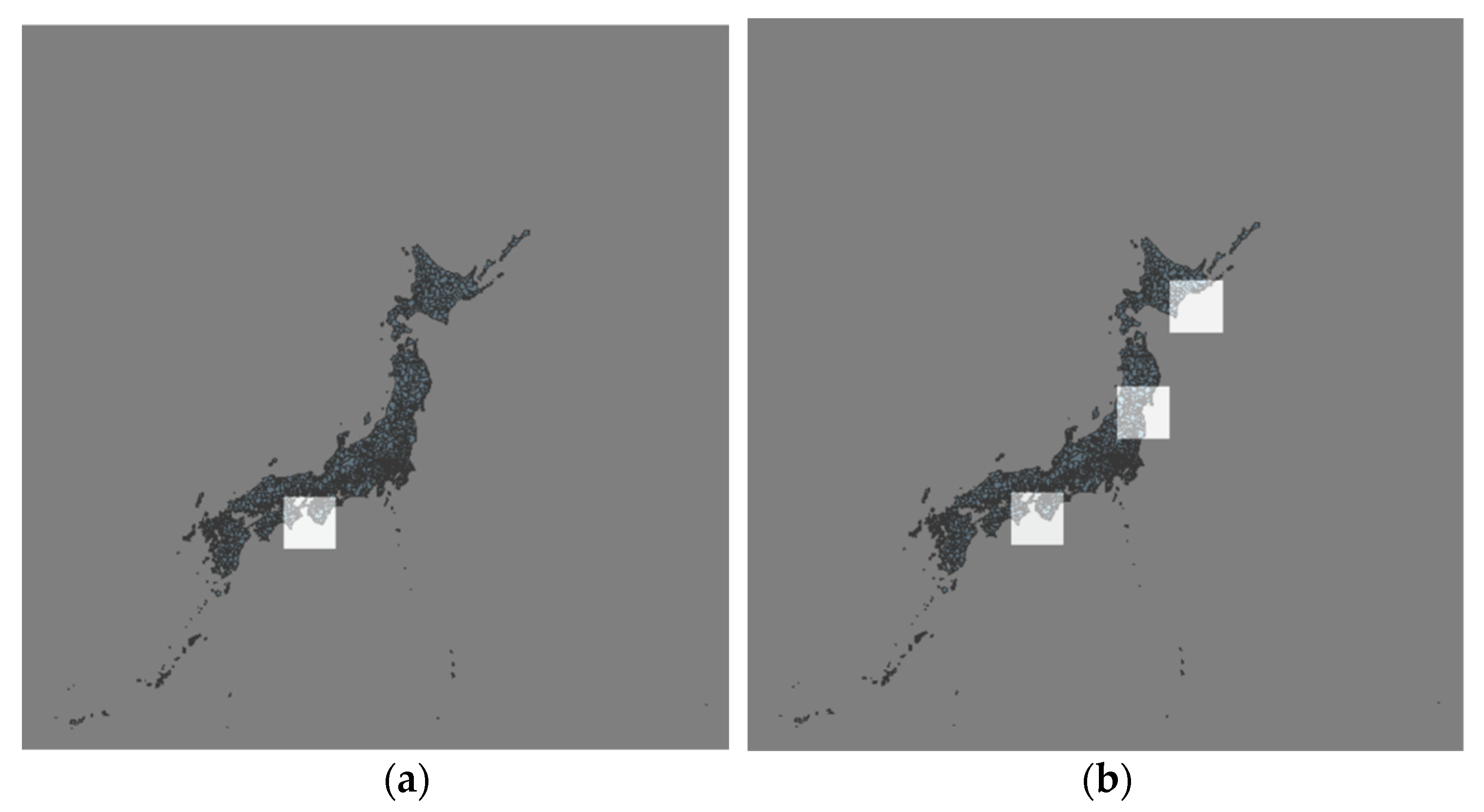
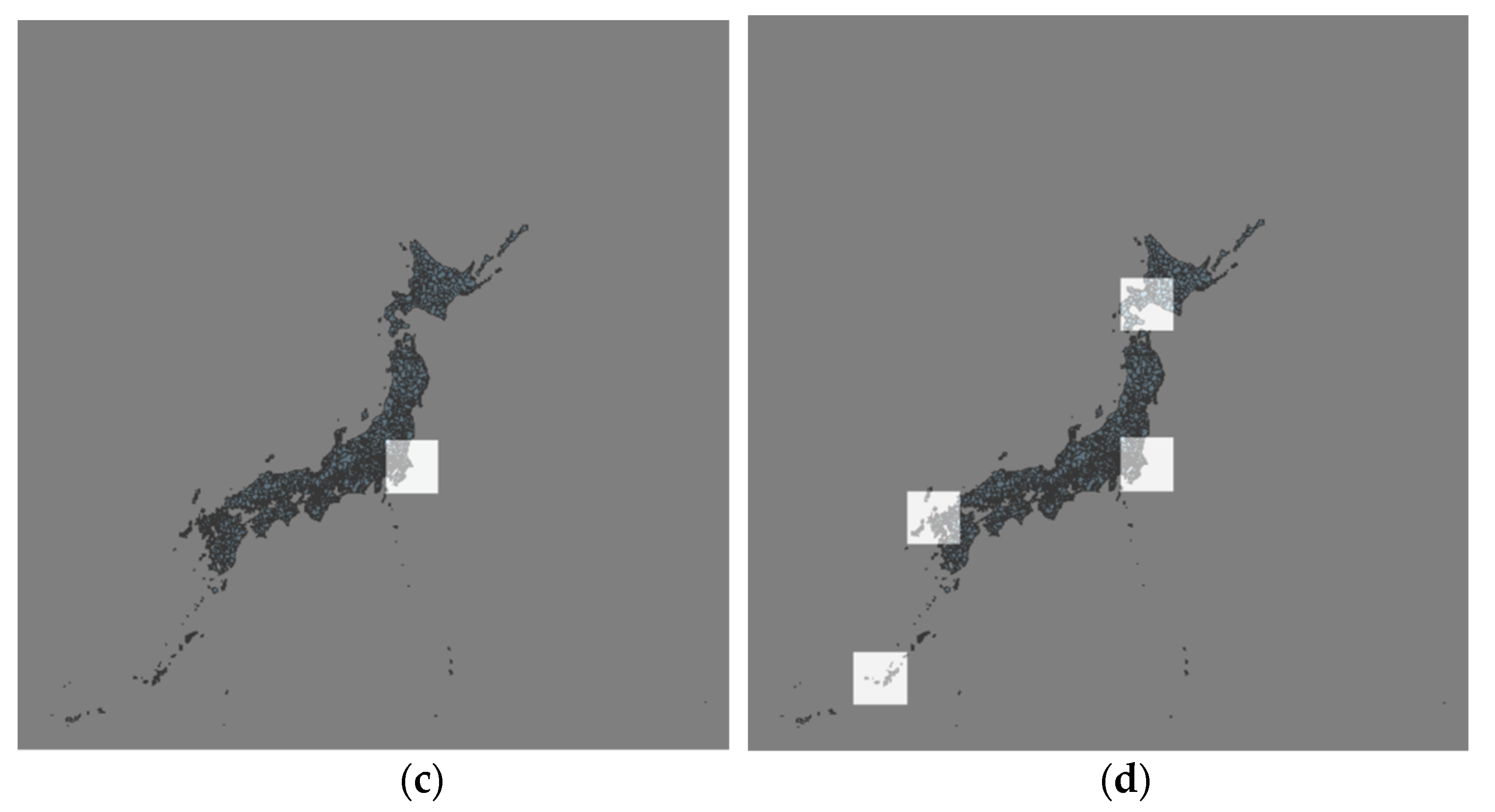
Figure 12 shows the earthquake prediction results of the trained SGMG-EEW on 21 July 2019 and 22 July 2019. Notably, the data for these two days do not belong to the dataset and have not been trained and tested. The results show that earthquake reports are missing in the prediction, consistent with the higher accuracy rate and lower recall rate in the experiment. However, although the accuracy of the earthquake prediction on the test set can reach 85%, the prediction accuracy of the new data is not ideal and there is still room for improvement.

5. Conclusions

This study focused on the problems of spatiotemporal association expression and deep learning-oriented computing in traditional layer-based data organization models against the background of spatiotemporal big data. A grid data organization method of multi-source spatiotemporal data based on GeoSOT was designed and SGMG-EEW was proposed. In addition, a deep learning verification experiment of the spatiotemporal correlation between multi-source spatiotemporal data (atmospheric anomalies and historical earthquakes) and earthquakes was conducted in Japan. The primary innovations are as follows.

(1)

A data organization model of a spatial datum grid (SGSM is a case) is established so that “data slices” can form “data blocks”; that is, different single layer spatial data types can form high-dimensional data vectors with a consistent data structure. This helps unify the deep learning of multi-source spatial information and improves the multi-source spatial information aggregation efficiency.

(2)

Based on the group convolution method, 3DGCNN-SGM is proposed, reducing the design and calculation costs of the multi-source spatial information deep learning model.

(3)

The experimental results on atmospheric anomalies and historical earthquakes in Japan show that the proposed SGMG-EEW can improve the deep learning effect of the spatiotemporal association between multi-source spatiotemporal data and earthquakes.

The accuracy of earthquake magnitude and location warning has significant room for improvement. Earthquake warning accuracy depends not only on the data organization model but also on the quantity and quality of seismic and its precursory data, as well as the deep learning model complexity. In the future, deep learning will be further improved by adding data including geographic factors such as the proximity to fault lines. More data types will be used in the SGSM proposed in this paper and the input dimension of 3DGCNN-SGM will be increased.

References

1. Devries, B.; Verbesselt, J.; Kooistra, L.; Herold, M. Robust monitoring of small-scale forest disturbances in a tropical montane forest using Landsat time series. Remote Sens. Environ. 2015, 161, 107–121. [Google Scholar] [CrossRef]
2. Zhang, P.; Gong, M.; Su, L.; Liu, J.; Li, Z. Change detection based on deep feature representation and mapping transformation for multi-spatial-resolution remote sensing images. ISPRS J. Photogramm. 2016, 116, 24–41. [Google Scholar] [CrossRef]
3. Chen, Z.; Huang, M.; Zhu, D.; Altan, O. Integrating remote sensing and a markov-FLUS model to simulate future land use changes in Hokkaido, Japan. Remote Sens. 2021, 13, 2621. [Google Scholar] [CrossRef]
4. Field, E.H.; Dawson, T.E.; Felzer, K.R.; Field, E.H.; Dawson, T.E.; Felzer, K.R.; Frankel, A.D.; Gupta, V.; Jordan, T.H.; Parsons, T.; et al. Uniform California Earthquake Rupture Forecast, Version 2 (UCERF 2). Bull. Seismol. Soc. Am. 2009, 99, 2053–2107. [Google Scholar] [CrossRef] [Green Version]
5. Gutenberg, B.; Richter, C. Seismicity of the Earth. In Seismicity of the Earth. Geological Society of America; Special Papers. No. 34; Geological Society of America: New York, NY, USA, 1941; pp. 1–126. [Google Scholar]
6. Yegulalp, T.M.; Kuo, J.T. Statistical prediction of the occurrence of maximum magnitude earthquakes. Bull. Seismol. Soc. Am. 1974, 64, 393–414. [Google Scholar] [CrossRef]
7. Lennartz, S.; Bunde, A.; Turcotte, D.L. Modelling seismic catalogues by cascade models: Do we need long-term magnitude correlations? Geophys. J. Int. 2011, 184, 1214–1222. [Google Scholar] [CrossRef] [Green Version]
8. Zhou, W.; Dong, H.; Liang, Y. The deterministic dendritic cell algorithm with Haskell in earthquake magnitude prediction. Earth Sci. Inform. 2020, 13, 447–457. [Google Scholar] [CrossRef]
9. Wang, T.; Wang, X.A.; Yong, S.; Xie, Z.; Guo, Z.; Lin, K. A sensor of ground temperature and its application in big earthquake monitoring. S. China J. Seismol. 2014, 34, 33–37. [Google Scholar]
10. Huang, F.; Li, M.; Ma, Y.; Han, Y.; Tian, L.; Yan, W.; Li, X. Studies on earthquake precursors in China: A review for recent 50 years. Geod. Geodyn. 2017, 8, 1–12. [Google Scholar] [CrossRef]
11. Fujiwara, H.; Kamogawa, M.; Ikeda, M.; Liu, J.Y.; Sakata, H.; Chen, Y.I.; Ofuruton, H.; Muramatsu, S.; Chuo, Y.J.; Ohtsuki, Y.H. Atmospheric anomalies observed during earthquake occurrences. Geophys. Res. Lett. 2004, 31. [Google Scholar] [CrossRef]
12. Alves, E.I. Earthquake forecasting using neural networks: Results and future work. Nonlinear Dyn. 2006, 44, 341–349. [Google Scholar] [CrossRef]
13. Asencio-Cortés, G.; Martínez-Álvarez, F.; Morales-Esteban, A.; Reyes, J.; Troncoso, A. Improving earthquake prediction with principal component analysis: Application to Chile. In International Conference on Hybrid Artificial Intelligence Systems; Springer: Cham, Germany, 2015; pp. 393–404. [Google Scholar]
14. Reyes, J.; Morales-Esteban, A.; Martínez-Álvarez, F. Neural networks to predict earthquakes in Chile. Appl. Soft Comput. 2013, 13, 1314–1328. [Google Scholar] [CrossRef]
15. Devries, P.M.R.; Viégas, F.; Wattenberg, M.; Meade, B.J. Deep learning of aftershock patterns following large earthquakes. Nature 2018, 560, 632–634. [Google Scholar] [CrossRef] [PubMed]
16. Mosavi, M.R.; Kavei, M.; Shabani, M.; Khani, Y.H. Interevent times estimation of major and continuous earthquakes in Hormozgān region based on radial basis function neural network. Geod. Geodyn. 2016, 7, 64–75. [Google Scholar] [CrossRef] [Green Version]
17. Asencio-Cortés, G.; Martínez-Álvarez, F.; Troncoso, A.; Morales-Esteban, A. Medium–large earthquake magnitude prediction in Tokyo with artificial neural networks. Neural Comput. Appl. 2017, 28, 1043–1055. [Google Scholar] [CrossRef]
18. Panakkat, A.; Adeli, H. Neural network models for earthquake magnitude prediction using multiple seismicity indicators. Int. J. Neural Syst. 2007, 17, 13–33. [Google Scholar] [CrossRef]
19. Martínez-Álvarez, F.; Reyes, J.; Morales-Esteban, A.; Rubio-Escudero, C. Determining the best set of seismicity indicators to predict earthquakes. Two case studies: Chile and the Iberian Peninsula. Knowl. Based Syst. 2013, 50, 198–210. [Google Scholar] [CrossRef]
20. Asim, K.M.; Martínez-Álvarez, F.; Basit, A.; Iqbal, T. Earthquake magnitude prediction in Hindu Kush region using machine learning techniques. Nat. Hazards. 2017, 85, 471–486. [Google Scholar] [CrossRef]
21. Wang, Q.; Guo, Y.; Yu, L.; Li, P. Earthquake prediction based on spatiotemporal data mining: An LSTM network approach. IEEE Trans. Emerg. Top. Comput. 2017, 8, 148–158. [Google Scholar] [CrossRef]
22. Huang, J.; Wang, X.; Zhao, Y.; Xin, C.; Xiang, H. Large earthquake magnitude prediction in Taiwan based on deep learning neural network. Neural Netw. World 2018, 28, 149–160. [Google Scholar] [CrossRef]
23. Shah, M.; Tariq, M.A.; Naqvi, N.A. Atmospheric anomalies associated with Mw > 6.0 earthquakes in Pakistan and Iran during 2010–2017. J. Atmos. Sol.-Terr. Phys. 2019, 191, 105056. [Google Scholar] [CrossRef]
24. Goodfellow, I.; Bengio, Y.; Courville, A. Deep Learning; MIT Press: Cambridge, MA, USA, 2016. [Google Scholar]
25. Huang, M.; Chen, N.; Du, W.; Wen, M.; Zhu, D.; Gong, J. An on-demand scheme driven by the knowledge of geospatial distribution for large-scale high-resolution impervious surface mapping. GISci. Remote Sens. 2021, 58, 562–586. [Google Scholar] [CrossRef]
26. Zhu, D.; Cheng, C.; Zhai, W.; Li, Y.; Li, S.; Chen, B. Multiscale spatial polygonal object granularity factor matching method based on BPNN. ISPRS Int. J. Geo Inf. 2021, 10, 75. [Google Scholar] [CrossRef]
27. Chen, Y.; Li, C.; Ghamisi, P.; Jia, X.; Gu, Y. Deep fusion of remote sensing data for accurate classification. IEEE Geosci. Remote Sens. Lett. 2017, 14, 1253–1257. [Google Scholar] [CrossRef]
28. Xu, Y.; Du, B.; Zhang, L. Multi-source remote sensing data classification via fully convolutional networks and post-classification processing. In Proceedings of the IGARSS2018 IEEE International Geoscience and Remote Sensing Symposium, Valencia, Spain, 22–27 July 2018; pp. 3852–3855. [Google Scholar]
29. Ienco, D.; Interdonato, R.; Gaetano, R.; Minh, D.H.T. Combining Sentinel-1 and Sentinel-2 Satellite Image Time Series for land cover mapping via a multi-source deep learning architecture. ISPRS J. Photogramm. 2019, 158, 11–22. [Google Scholar] [CrossRef]
30. Hang, R.; Li, Z.; Ghamisi, P.; Hong, D.; Xia, G.; Liu, Q. Classification of hyperspectral and LiDAR data using coupled CNNs. IEEE Trans. Geosci. Remote Sens. 2020, 58, 4939–4950. [Google Scholar] [CrossRef] [Green Version]
31. Hong, D.; Gao, L.; Yokoya, N.; Yao, J.; Chanussot, J.; Du, Q.; Zhang, B. More diverse means better: Multimodal deep learning meets remote-sensing imagery classification. IEEE Trans. Geosci. Remote Sens. 2020, 59, 4340–4354. [Google Scholar] [CrossRef]
32. Cheng, C.; Ren, F.; Guoliang, P. Introduction to Spatial Information Subdivision and Organization; Science Press: Beijing, China, 2012. (In Chinese) [Google Scholar]
33. Li, Q.; Nevalainen, P.; Peña Queralta, J.P.; Heikkonen, J.; Westerlund, T. Localization in unstructured environments: Towards autonomous robots in forests with delaunay triangulation. Remote Sens. 2020, 12, 1870. [Google Scholar] [CrossRef]
34. Murai, S. Can we predict earthquakes with GPS data? Int. J. Digit. Earth. 2010, 3, 83–90. [Google Scholar] [CrossRef]
35. Liu, Z.N.; Yu, X.Y.; Jia, L.F.; Wang, Y.S.; Song, Y.C.; Meng, H.D. The influence of distance weight on the inverse distance weighted method for ore-grade estimation. Sci. Rep. 2021, 11, 1–8. [Google Scholar]
36. Xie, S.; Girshick, R.; Dollár, P.; Tu, Z.; He, K. Aggregated residual transformations for deep neural networks. In Proceedings of the IEEE Conference on Computer Vision and Pattern Recognition, Honolulu, Hawaii, 21–26 July 2017; pp. 1492–1500. [Google Scholar]
37. Kataoka, H.; Wakamiya, T.; Hara, K.; Satoh, Y. Would mega-scale datasets further enhance spatiotemporal 3d CNNs? arXiv Prepr. 2020, arXiv:2004.04968. [Google Scholar]
38. Hara, K.; Kataoka, H.; Satoh, Y. Learning spatiotemporal features with 3d residual networks for action recognition. In Proceedings of the IEEE International Conference on Computer Vision Workshops, Venice, Italy, 22–29 October 2017; pp. 3154–3160. [Google Scholar]
39. Mohri, M.; Rostamizadeh, A.; Talwalkar, A. Foundations of Machine Learning; MIT Press: Cambridge, MA, USA, 2018. [Google Scholar]
Figure 1. Overall structure of the study.
Remotesensing 13 03426 g001
Figure 2. Determination process of GeoSOT subdividing level of seismic sample grid.
Remotesensing 13 03426 g002
Figure 3. Spatiotemporal grid interpolation: grid interpolation of atmospheric anomalies on 1 June 2018.
Remotesensing 13 03426 g003
Figure 4. Schematic of group convolution principle. (a) Ordinary convolution. (b) Group convolution.
Remotesensing 13 03426 g004
Figure 5. Schematic of 3D-GridResNet-18 network architecture.
Remotesensing 13 03426 g005
Figure 6. Schematic of experimental data. (a) True seismic values on 20 July 2019. (b) Spatial distribution of meteorological stations in Japan.
Remotesensing 13 03426 g006
Figure 7. Training loss function curve of the experimental group.
Remotesensing 13 03426 g007
Figure 8. Mean and variance of the training loss function curves of AA-C.
Remotesensing 13 03426 g008
Figure 9. Mean and variance of the training loss function curves of HE-C.
Remotesensing 13 03426 g009
Figure 10. Mean and variance of the training loss function curves of NG-C.
Remotesensing 13 03426 g010
Figure 11. Model (SGMG-EEW, AA-C, HE-C, NG-C, SVM-C, and SSA-C) prediction accuracies.
Remotesensing 13 03426 g011
Figure 12. Earthquake prediction results of the trained SGMG-EEW on 21 July 2019 and 22 July 2019. (a) Prediction on 21 July 2019. (b) Ground truth on 21 July 2019. (c) Prediction on 22 July 2019. (d) Ground truth on 22 July 2019.
Remotesensing 13 03426 g012aRemotesensing 13 03426 g012b