Abstract
Water level (WL) and terrestrial water storage (TWS) are two important indicators for early alerts of hydrological extremes. Their variation is governed by precipitation under monsoon variability, in particular in the Mekong river basin, where it is affected by the interaction between the Indian summer monsoon (ISM) and western North Pacific monsoon (WNPM). This study aimed to quantify the contributions of two monsoons to the water levels of four hydrological stations (i.e., My Thuan, Can Tho, Chau Doc and Tan Chau) on the Mekong Delta and the terrestrial water storage of the entire Mekong River basin through relative importance analysis. Three methods—multivariate linear regression; Lindeman, Merenda and Gold (LMG); and the proportional marginal variance decomposition (PMVD) methods—were selected to quantitatively obtain the relative influence of two monsoons on water level and TWS. The results showed that, from 2010 to 2014, the proportions of the ISM impacts on the water level obtained with the three methods ranged from 55.48 to 81.35%, 50.69 to 57.55% and 55.41 to 93.64% via multivariate linear regression, LMG and PMVD, respectively. Further analysis showed that different choices of time spans could lead to different results, indicated that the corresponding proportion would be influenced by other factors, such as El Niño–Southern Oscillation (ENSO). The removal of ENSO further enlarged the relative importance of the ISM, and the mean values of the four stations were increased by 8.78%, 2.04% and 14.92%, respectively, via multivariate linear regression, LMG and PMVD. Meanwhile, based on the analysis of terrestrial water storage, it was found that the impact of the ISM on the whole Mekong River basin was dominant: the proportions of the impact of the ISM on terrestrial water storage increased to 68.79%, 54.60% and 79.43%, which rose by 11.24%, 2.96% and 19.77%, respectively, via linear regression, LMG and PMVD. The increases almost equaled the quantified proportion for the ENSO component. Overall, the novel technique of quantifying the contributions of monsoons to WL and TWS can be applied to the influence of other atmospheric factors or events on hydrological variables in different regions.
1. Introduction
Monsoons are one of the most energetic components of the earth’s climate system [1], affecting the livelihoods of more than 60% of the world population [2]. Recently, many research studies have revealed the relationship between the Asian summer monsoon and hydrological extreme events. For instance, the Asian monsoon is the key factor affecting the occurrence of drought and flood across different regions in India [3] and China [4] and the biogeochemical and hydrological processes in South Korea [5]. The Indian summer monsoon (ISM) and western North Pacific monsoon (WNPM) are the two main monsoon members in Asia that have significant influences on Southeast Asia. Two circulation indices, the ISM and WNPM [1], are normally selected to explain the regional hydrological and climatic conditions.
Various research studies have demonstrated that a significant interaction between the Asian monsoon and El Niño–Southern Oscillation (ENSO) exists [1,6,7]. For example, the East Asian summer monsoon is influenced by El Niño events, leading to more precipitation in the summer after El Niño for some regions [8]. Significant negative correlations have been found between the WNPM and ISM during the El Niño early onset years and during the El Niño decaying summer [9]. In fact, the respective relationships between ENSO and precipitation [10] and water levels [11] in the Mekong River basin have also been analyzed, and it was found that hydrological variables are significantly influenced by ENSO events. Applying the above findings, recent studies have been focused on water level reconstruction based on ENSO [12], drought indices and satellite gravimetry [13]. However, the quantification of the relative impacts of the above two monsoons on the water level and terrestrial water storage have never been reported.
As the largest river in Southeast Asia [14], the Mekong River basin (MRB), with a total basin covering an area of 795,000 across 25° of latitude [15], discharges freshwater southward from China, flowing through Myanmar, Laos, Thailand, Cambodia and Vietnam [16] to the South China Sea (SCS) [17] (Figure 1). The MRB is normally divided into two parts: the Upper Mekong basin in China (called the Lancang River) and the Lower Mekong basin beginning from the Chinese boundary and extending to the SCS. The terrain in the upper basin is steep and narrow but becomes relatively flat and open in the lower basin, especially from Cambodia to the SCS [17]. The climate of the MRB is significantly affected by the Asian–Pacific monsoon system [18], especially the downstream MRB. The MRB ranks tenth among the global megabasins on the basis of mean annual discharge at the estuary mouth [19], which is inhabited by around 65 million people [17]. Due to the Asian–Pacific monsoon system, the climate of the MRB presents obvious dry (from early May to October) and wet (from November to April) seasons [20], controlled by the cold air from the Eurasian continent and the summer monsoon by air from both the southwest and the southeast. Water discharge (WD) mainly comes from the rainfall in the rainy season in the downstream MRB [12].
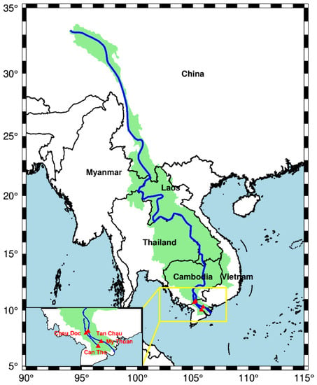
Figure 1.
Map of Mekong basin with two pairs of selected hydrological stations (My Thuan and Can Tho, and Chau Doc and Tan Chau) located in the Mekong Delta.
WD monitoring is significantly important for managing water resources and obtaining alerts about hydrological extremes that can cause otherwise unforeseeable losses to the economy [21,22,23]. As a power function of the WD [24,25], the water level (WL) has an inseparable relationship with people’s lives, production and even regional development. Given the high correlation with the precipitation, whether on land [26], lakes [27], or rivers [28,29], the WL and terrestrial water storage (TWS) are affected by precipitation and discharge through the monsoon, as this large-scale atmospheric circulation controls the spatiotemporal variability of precipitation [30].
As a key part of terrestrial water resources [31], the TWS, consisting of surface water storage (e.g., reservoirs and lakes), groundwater, soil moisture, snow and ice [32], can be inferred from Gravity Recovery and Climate Experiment (GRACE). This provides a synoptic view of its spatiotemporal variability [33], which can better reflect the change of terrestrial water quantity at a regional scale when compared to WL. It plays a major role in the exchange of water mass between the atmosphere and the ocean [34]. The TWS variability can be attributed to precipitation [35,36], evapotranspiration [35] and ice melting, to mention only a few factors [36]. Monsoons’ effects on TWS have been investigated recently. He et al. [37] discovered that the shifting of TWS spatial distribution over East China is due to the varying strengths of local winds and Asian monsoons. On the other hand, the variability of TWS across China has long been attributed to the interaction of monsoons and a connection with El Niño–Southern Oscillation (ENSO); for instance, by Long et al. [38], Ni et al. [39], Tang et al. [40] and Zhang et al. [41]. Several research studies have quantitatively inferred that WL variations are linked to the TWS (e.g., [42,43,44]). For example, WLs have been reconstructed based on TWS and other indices in the Mekong and Yangtze river basins [13,45]. Though the relationship between WL and TWS has been scientifically investigated and the practical applications of the relationship have been explored, the direct comparison between the WL and TWS as affected by monsoons has rarely been studied, let alone the quantification of the relative importance (or contribution) of the governing monsoons for the WL and TWS.
This study aimed to quantify the influences of the ISM and WNPM on the WL of the Mekong Delta and the TWS in the MRB. Linear regression and relative importance (RI) analyses of long periods and continuous short periods were used to calculate their relative influence. The RI is a statistical tool for quantifying the relative contribution of each potential explanatory variable (i.e., regressor) comprising the value of [46,47,48]. After preprocessing, the relative importance of the ISM and WNPM indices for the WL and TWS was calculated with a multivariate linear model; the Lindeman, Merenda and Gold (LMG) model; and the proportional marginal variance decomposition (PMVD) model. Moreover, the relative importance of the data after removing the signal related to ENSO with wavelet transform coherence (WTC) was also analyzed. The results were compared to analyze the effect of ENSO on WL and TWS.
This article is structured as follows: The dataset is described in detail in Section 2, and the research methods and evaluation indicators are stated in Section 3, followed by the results of linear regression, LMG and PMVD in Section 4, with WTC used as well. The results are further analyzed also in Section 4 and the conclusion is given in Section 5.
2. Datasets Description
2.1. Water Level Data
Daily WLs from 1 January 2008 to 31 December 2015 observed at four hydrological stations (i.e., My Thuan and Can Tho, approximately 80–110 km from the estuary mouth, and Chau Doc and Tan Chau, approximately 220 km from the estuary mouth) were obtained from the Mekong River Commission (MRC; http://www.mrcmekong.org, accessed on 10 July 2020). Four station time series are displayed in Figure 2, with their basic information given in Table 1. In this study, the data time span for 2010–2014 was taken as an example for our initial investigation, and the rest were used for subsequent comparison and analysis.
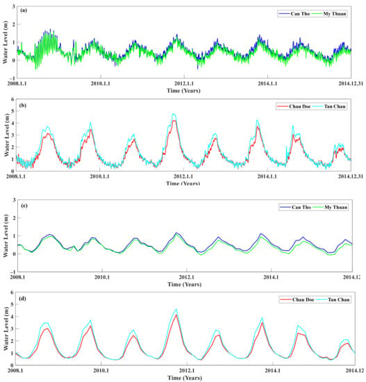
Figure 2.
WLs of four selected stations in the Mekong River delta (MRD): (a,b) are the daily observed WLs and (c,d) are the WLs after monthly averaging.

Table 1.
Maxima, minima, means and standard deviations of daily observed (and monthly averaged) WLs from four selected stations in the MRD.
The WL presented obvious annual periodic changes due to the seasonal precipitation and even monsoon activities [13]. Periodic changes were accompanied by small diurnal fluctuations, which are mainly caused by dominant semi-diurnal ocean tides in the southern SCS [49,50]. For Can Tho and My Thuan, which are closer to the coast, the backwater from the ocean intrudes into the estuary, which should dampen the amplitude of the WL [49]. As a result, the standard deviations of the WL at My Thuan and Can Tho were smaller than that at the upper pair of stations (i.e., Chau Doc and Tan Chau) (Table 1). To be consistent with the monthly monsoon index and basin-averaged TWS, monthly averaging was conducted to smooth the raw data [49] (Figure 2), and the statistics of the monthly averaged data are shown in Table 1 as well.
2.2. Indian Summer Monsoon (ISM) Index and Western North Pacific Monsoon (WNPM) Index
To numerically represent the intensity of the tropical westerly monsoon, the Indian summer monsoon (ISM) index and western North Pacific monsoon (WNPM) index [1] were used. The ISM index is defined by a difference of 850 hPa in the zonal winds between 5–15°N, 40–80°E and 20–30°N, 70–90°E, whereas the WNPM index is defined by a difference of 850 hPa in the westerlies between 5–15°N, 100–130°E and 20–30°N, 110–140°E [1], as shown in Figure 3. The 850 hPa zonal wind was used as an indicator because it better reflects the variations of the corresponding convective heating [51], from which the monsoon can be formed.
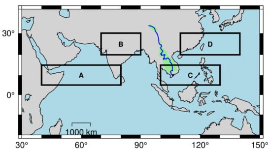
Figure 3.
The definitions of the ISM index (a difference of 850 hPa in zonal winds between A and B, i.e., ) and WNPM index (a difference of 850 hPa in westerly winds between C and D, i.e., ).
The time series of the ISM index and WNPM index from 2003 to 2015 can be directly accessed at the website of the Asia-Pacific Data-Research Center (APDRC) (http://apdrc.soest.hawaii.edu/projects/monsoon/realtime-monidx.html, accessed on 10 July 2020), as displayed in Figure 4. Both indices display the obvious annual cycle and short-term fluctuations, similar to those for the WL.
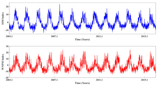
Figure 4.
Indian summer monsoon (ISM) index and western North Pacific monsoon (WNPM) index from 2003 to 2015. A positive ISM index means that the monsoon activity in region A is stronger than that in region B (Figure 3), and the negative value indicates the opposite. A positive WNPM index means that the monsoon activity in region C is stronger than that in region D (Figure 3), and the negative value indicates the opposite.
2.3. Terrestrial Water Storage Data
The Gravity Recovery and Climate Experiment (GRACE) yields time-variable TWS data on a monthly scale [52]. The TWS data used here, with a theoretical spatial resolution of 3°, were computed from the CSR GRACE Level 2 Release 05 (RL05) GSM monthly gravity fields, accessible at the website of the Center of Space Research (CSR) managed by NASA (http://www2.csr.utexas.edu/grace/RL05.html, accessed on 10 July 2020). Two post-processing steps were applied to obtain TWS data from the GRACE gravity spherical harmonic coefficients. The GRACE term was replaced by satellite laser ranging (SLR) and degree-one terms were restored to correct for geocenter motion [53,54], followed by a de-striping process and Gaussian filtering with a radius of 350 km [55,56]. The data time series of the Mekong River basin were then spatially averaged to obtain a single TWS time series for the entire Mekong basin for the period from 2003 to 2015, as given in Figure 5.
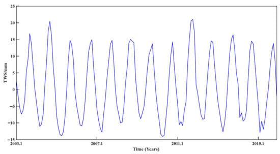
Figure 5.
TWS time series for the entire Mekong basin for the period from 2003 to 2015.
2.4. Multivariate ENSO Index (MEI)
As a wind field and sea surface temperature oscillation occurs in the equatorial eastern Pacific region, ENSO can be detected from the anomalies of sea-level pressure difference and sea surface temperature (SST) [57]. In this study, the multivariate ENSO index (MEI) was considered as a more integrated index than other ENSO indices for the quantification of the strength and variability of ENSO [58] because the MEI is calculated based on the sea surface pressure, the zonal and meridional components of the surface wind, the SST and the total cloudiness fraction of the sky over the tropical Pacific [30]. The MEI dataset was downloaded on 10 July 2020 at http://www.esrl.noaa.gov/psd/enso/mei.ext/table.ext.html.
3. Method and Evaluation Metrics
3.1. Research Flow
The flow of this study included the following aspects: pretreatment (including time lag analysis); calculation of the relative contributions of the ISM and WNPM via linear regression, LMG and PMVD; and removal of the ENSO effect from the monsoon index through WTC (Figure 6).
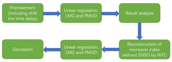
Figure 6.
The research flowchart of this study.
3.2. Time Lag Analysis
Considering that only the quantitative relationship between the monsoon index and water level was explored, a time lag between them must exist (Figure 7). This is because time is required for the monsoonal wind to generate the process that, through precipitation (recharge)–storage–discharge, ultimately affects the water level at the estuary. Cross-correlation was employed to align the time series [59], defined as
where and are time series of length means the i-th sample of the time series and means the k-th number of the cross-correlation. The cross-correlation is maximized when the time series and are aligned well with a time lag between them. For instance, in this study, is the monsoon index and is the WL or TWS, and is maximized when the monsoon index and WL or TWS are aligned well with a time lag between them.
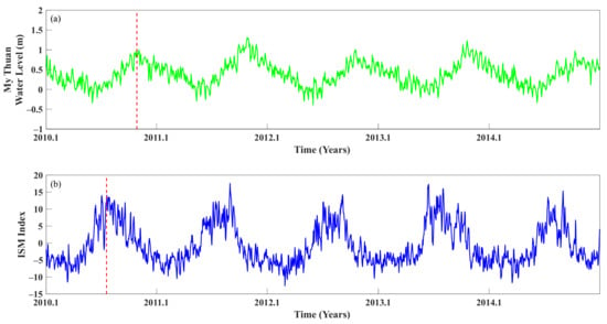
Figure 7.
Time lag between (a) WL at My Thuan and (b) Indian summer monsoon index.
The degree of the maximum value of , denoted as is the parameter used to calculate time lag, , as follows:
where stands for the time lag and is the sampling interval of the time series. The lag is positive when time series occur later than that of time series . The time lag between the monsoon index and the daily WL observed at station (monthly basin-averaged TWS), with the in terms of the day (respectively, month), was calculated (Table 2).

Table 2.
The time lag between the monsoon index and WL (or basin-averaged TWS).
The time lags of the WNPM for four selected stations were all shorter than those of the ISM except the one at Can Tho. This indicates that the influence of the WNPM arrives earlier than that of the ISM. This might be attributable to the defined zone of the WNPM being 1500 km closer to the location of the MRB, as shown in Figure 3.
Differently from the daily WL fluctuation resulting purely from the land surface hydrology, the long-period ocean tides, such as semi-annual and annual tidal constituents, play an important role in providing a backwater effect on the WL at the river mouth, such that the effect of the monsoon is not reflected instantly. Consequently, the time series for the station pair closer to the ocean (i.e., My Thuan and Can Tho) presented a longer time lag (i.e., ~3 months) than that of the upper station pair (i.e., Chau Doc and Tan Chau). Compared to the difference between the time lags of the two station pairs, that of the two monsoon indices was relatively small at the same station. For instance, 9 day and 3 day time lags were present at My Thuan and Can Tho, and 16 day and 21 day time lags were present at Chau Doc and Tan Chau.
3.3. RI Calculated from Linear Regression Coefficients
A multivariate linear model is commonly used to quantify the relationships among different variables. For a dependent variable and multiple independent variables , the basic linear model is
where is the constant offset, are the coefficients for each independent variable and is the random error with a mathematical expectation that equals zero. According to Equation (3), the quantitative relationship between the WLs at stations and the two monsoon (ISM and WNPM) indices can be formulated as follows:
Therefore, the relative importance (or contribution) of each monsoon index can be calculated as
3.4. Evaluation Indices
The Pearson correlation coefficient (PCC) was selected to evaluate the performance of the WL modeled from the linear regression against the observed one. Its definition is shown in Equation (6), where and represent the WL/TWS from observation and from the linear regression based on monsoon indices, respectively. refers to the mean of , so too does .
Additionally, two other metrics were also selected: the normalized root mean squared error (NRMSE) and the Nash–Sutcliffe efficiency model (NSE). The NRMSE, as an indicator to reflect the accuracy in normalized form, is defined as follows:
The NSE, which was first introduced by Nash and Sutcliffe in 1970 [60], is a widely used coefficient for the evaluation of hydrological models against observed data, with a range from −∞ to 1. The numerical value of the NSE reflects the best performance of the model when it approaches 1. It can be calculated as Equation (8) shows.
3.5. RI from Linear Regression Using LMG and PMVD Methods
Since the RI refers to the quantification of an individual regressor’s contribution to a multivariate linear model [61], assigning shares of “relative importance” to each one of a set of regressors is one of the keys to linear regression [62]. Choosing from among many methods for determining the RI, the Lindeman, Merenda and Gold (LMG) [63] and proportional marginal variance decomposition (PMVD) [64] methods were used here to decompose into the contributions of each regressor. refers to the coefficient of determination, which is defined as follows:
where is the observed value at time , and is the linear estimate of . is the average of the dependent variable and is the set of possible regressors contributing to the overall description of the dependent variable. In this study, stands for WL/TWS and consists of the ISM index and WNPM index; that is . In Section 4.4, MEI is added into as a possible factor as well. The LMG and PMVD methods eliminate the dependence of the contribution of regressors () by replacing orders of regressions and averaging marginal contributions of replaced regressors. Suppose represents the input of a set of regressors into the model, and represents different orders of in the model. The set of regressors before in order is denoted as . Consequently, the marginal contribution of the regressor in the order, denoted as , can be written as
With the LMG method, all s are simply averaged in the order , which is calculated as
where is the number of regressors in .
However, with the LMG method, when one regressor is related to other regressors, a biased marginal contribution is obtained, even if the regression coefficient of and the dependent variable is zero. Therefore, the PMVD method, which is a weighted analogue of the LMG method using data-dependent weights, has been proposed to solve this problem [64]. The data-dependent weights, , are derived from a set of axioms and used to weight the permutation in the PMVD method, which is defined as
3.6. Wavelet Transform Coherence
Wavelet transform coherence (WTC), first put forward by Torrence and Webster (1999) [65], has been widely used in time series analysis [66,67]. The continuous wavelet transform (CWT) is one class of wavelet transforms. The CWT of the time series of the index, for example, with length and uniform time step , can be defined as , which is a convolution of the with the scaled and normalized wavelet [67]:
where represents the time index and is the wavelet scale. The is a particular wavelet basis, called the Morlet wavelet, defined as:
where is the dimensionless frequency and is the dimensionless time. Aiming at striking a good balance between frequency and time, the was chosen to be 6 [68].
According to [27], the cross-wavelet spectrum of two time series, for example, and , can be defined as :
Here, represents the complex conjugate. Then, according to [31], the WTC of these two time series, , can be calculated as:
Here, is a smoothing operator. The significance level of the WTC can be calculated using the Monte Carlo method. The phase difference is:
4. Results and Discussion
4.1. RI Analysis from Linear Regression, LMG and PMVD
The results obtained from the multivariate linear model are shown in Table 3. Although the defined boundary of the WNPM index was closer to the MRD (Figure 3), the contribution of the ISM to the water level was larger than that of WNPM at the estuary. Combined with the geographical locations of the hydrological stations (Figure 1), it can be seen that the contributions of the two monsoons to the WL varied considerably. This was particularly apparent for the pair consisting of My Thuan and Can Tho, where the contribution ratio of the ISM and WNPM was four to one (i.e., 4:1). From east to west, the relative contribution of the ISM decreased from 81% to 55%, while that of the WNPM increased. This implies that the WL at stations closer to the open ocean (i.e., Can Tho and My Thuan) was subject to a stronger influence from the ISM. The contribution ratio of the ISM index for the TWS was similar to the results for the WL for Chau Doc and Tan Chau, the reason being that a basin-averaged TWS was employed. For the influence on both the WL and on the TWS, the contribution of the ISM was larger than that of WNPM (Table 3), implying that the ISM plays a stronger role.

Table 3.
The RI of the ISM and WNPM indexes generated from the multivariate linear models.
In terms of evaluation metrics (i.e., PCC, NRMSE and NSE), it can be seen from Table 4 that the ISM and WNPM were, to a large extent, able to explain the fluctuation of the WL and basin-averaged TWS via the multivariate linear model in Equation (3). Therefore, the analyses of the relative contributions of the ISM and WNPM seem to have been appropriate. Among these analyses, the data fitting based on the basin-averaged TWS appears to have been the best (the PCC was 0.9482, the NRMSE was 0.0905 and the NSE was 0.8990). However, the WL obtained by the linear model was not in fact completely consistent with the actual measurement results (Figure 8), most obviously at the peak and the trough. For instance, the peak of observed TWS during 2011–2012 was lower than that of the model based on monsoon indices, as was that of the WL. This could be attributed to the influence of a medium La Niña event in 2010–2012, which might have increased the water in the MRB [8,10], leading to the higher values for the WL and TWS. Therefore, the model with only two monsoon indices could not precisely reconstruct the specific changes in the WL and TWS.

Table 4.
Results of relative importance analysis for the two monsoons with regard to the WL and TWS.
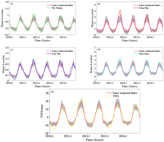
Figure 8.
WL and linear regression fitting for the period from 2010 to 2014 at (a) My Thuan, (b) Chau Doc, (c) Can Tho and (d) Tan Chau, along with (e) the TWS and its linear regression fitting for the period from 2010 to 2014.
The RI of the ISM and WNPM resulting from the LMG and PMVD methods was also calculated (Table 4). Compared to the multivariate linear regression result (Table 4), the proportions of RI for the ISM and WNPM resulting from the LMG and PMVD methods for the TWS were almost the same. For the WL, the total response variances at My Thuan and Can Tho were much smaller compared to those at Chau Doc and Tan Chau. This was due to the difference in amplitudes. The proportion of variance explained by the model, expressed as , was relatively similar. Although the difference between the LMG and PMVD methods lies in the data-dependent weights of the PMVD, the results generated from both methods were very different from each other, especially for the WL at My Thuan and Can Tho.
With respect to the results from Table 4, the resulting proportions of RI for My Thuan and Can Tho yielded high consistency with each other when using the LMG method, and the RI of the ISM accounted for more than 57%. However, the RI of the ISM was about equal to that of the WNPM at Chau Doc and Tan Chau. For the results generated from the PMVD, the proportions of RI of the ISM at the four stations for the WL were higher than those of the LMG, especially at My Thuan (36.09% higher) and Can Tho (25.51% higher).
4.2. Comparison among Three Methods
Comparing Table 3 with Table 4, it can be seen that similarities and differences existed among the results generated from different RI methods. Taking the results for the WL as an example, the ISM accounted for a larger relative contribution to WL than the WNPM for all four stations. The ISM relative contribution to the WL at My Thuan and Can Tho was higher than at the other two stations. However, there were significant differences in the specific values: the results generated with multivariate linear regression were closer to those of the PMVD, especially in the pair consisting of Chau Doc and Tan Chau. The proportions of RI of the ISM at My Thuan and Can Tho obtained from multivariate linear regression were lower than those obtained with the PMVD method. For the LMG method, all the results were in favor of an equilibrium between the ISM and WNPM, and the proportions of the ISM at all stations were all lower than with the previous two methods.
In essence, it is the characteristics of the methods themselves that leads to different results. The three methods are fundamentally linear regression, which aims to measure the influence of each explanatory variable on a dependent variable. The first method, multivariate linear regression, is an ideal model based on the hypothesis that all explanatory variables are unrelated to each other. When considering the correlation between variables, the order in which variables participate should not be ignored during the model interpretation process. As stated in Section 3.4, the LMG method is simply the average of the marginal contributions of all permutations. Based on the LMG method, the PMVD method assigns different weights in different orders to ensure that variables with coefficients of zero do not participate in the relative importance calculation process. Consequently, as shown in Figure 9, the results of the LMG method tended to show more balance between the ISM and WNPM, whereas the PMVD method, on the other hand, highlighted the part with greater influence, reminding us of the factors dominantly related to the dependent variable. In addition, the resulting proportions of RI of the ISM and WNPM for the dependent variables obtained from the PMVD method and linear regression were relatively close, indicating that a direct relation between the ISM and WNPM did not exist.
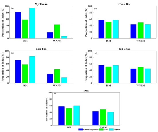
Figure 9.
The comparisons of different resulting proportions of RI for the ISM and WNPM in the period from 2010 to 2014 obtained by three methods (multivariate linear regression, LMG and PMVD) for the WL at (a) My Thuan, (b) Chau Doc, (c) Can Tho and (d) Tan Chau, along with (e) those for the TWS.
4.3. Influence of Different Data Time-Span Selections
The above results were based on five years of data from 2010 to 2014. To examine whether a change in the selected data time-span would produce different results, data spanning from 2008 to 2012 were employed.
For the RI of the ISM and WNPM for the WL, the ISM was obviously still dominant in the long term, but interannual fluctuations might exist (Table 5). Although the basic characteristics for the period from 2008 to 2012 were consistent with that for the period from 2010 to 2014, the proportions of RI of the ISM obtained with the three methods for the period from 2008 to 2012 were consistently larger than those for the period from 2010 to 2014. This was particularly apparent at Chau Doc and Tan Chau, where the contribution of the ISM to the WL increased by ~5% using the LMG method, while with multivariate linear regression (PMVD) it increased by ~15% (30%). Moreover, no significant changes were found in the RI results for My Thuan and Can Tho, especially when using the LMG method.

Table 5.
Results of different intervals. The percentage in brackets indicates the change of the value compared with that for the period from 2010 to 2014. The change of the WNPM is opposite that of the ISM.
However, the resulting proportions of RI of the ISM and WNPM for the TWS were quite different. During 2008–2012, the RI of the WNPM increased by 23.55%, 7.95% and 42.24%, as obtained via multivariate linear regression, LMG and PMVD, respectively, occupying the dominant position of influence on the TWS. Combined with the comprehensive performance results shown in Table 6, it can be seen that the change in the monsoons’ influence on the TWS was significantly larger than that on the WL.

Table 6.
Comparison of results before and after ENSO removal. The percentage in brackets indicates the change of the value compared with that before the ENSO signal was removed, which can be regarded as the influence proportion of ENSO. The change of the WNPM is opposite to that of the ISM.
To further explore the short-term proportions of RI of the ISM and WNPM for the WL and TWS, six (respectively, eleven) three-year time-spans for the period from 2008 to 2015 (respectively, 2003 to 2015) were selected with a rolling data window. We found that the results were not the same as the results shown in Table 5 (Figure 10). For the proportions of RI of the ISM and WNPM for the WL at the four stations in the estuary, those at My Thuan and Can Tho showed a consistent change pattern in the ISM contribution, in which they all decreased first, then increased, and then decreased again; this was also found at Chau Doc and Tan Chau. However, the times of the turning points were not exactly the same. This shows that the monsoons’ interactions varied with time. For example, the minimum RI of the ISM for the WL at My Thuan was in the period from 2009 to 2011, while that at Can Tho was in the period from 2010 to 2012. The results for My Thuan in the period from 2013 to 2015 were almost the same as for 2012–2014, whereas Can Tho showed a significant downward trend. As My Thuan and Can Tho are located in two main tributaries downstream of the Mekong Delta (Figure 1), we speculate that the length of the tributaries and the distance of the hydrologic stations from the estuary mouth might have led to the difference in the observed WL which was revealed in our results. The influence of the ISM on the TWS also fluctuated up and down, similar to the results for the WL. The results obtained with the LMG method were the most stable due to the simple averaging of the marginal contribution of each regressor. We speculate that ENSO might play a substantial role in the short-term variability in the strength of monsoons. This is further explored in a later section.
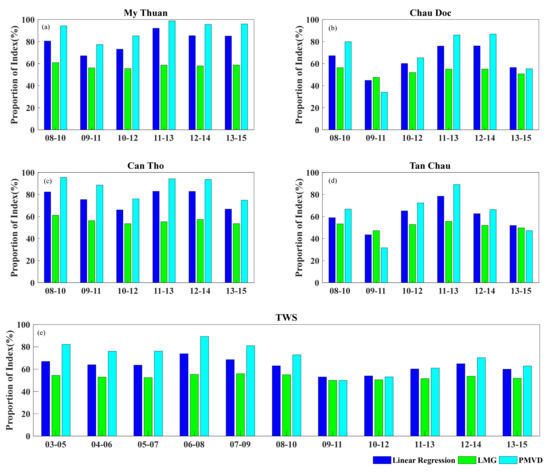
Figure 10.
The temporal changes of the ISM’s effects on the WL for six three-year time-spans for the period from 2008 to 2015 at: (a) My Thuan, (b) Chau Doc, (c) Can Tho and (d) Tan Chau, along with (e) that for the TWS for eleven three-year time-spans for the period from 2003 to 2015.
4.4. Influence of ENSO
Figure 10 indicated that the RI of the ISM for the WL had a change cycle, but the reasons for the periodicity were not clear, nor were those for the significant change in the monsoons’ influence on the TWS during the periods from 2008 to 2012 and 2010 to 2014 (Table 5). To explore the reasons behind the changes of influence, the MEI index was further incorporated into the linear regression analysis. After introducing the MEI index, the influence proportions for the changes in the WL and TWS were calculated using the same methods (Figure 11 and Figure 12).
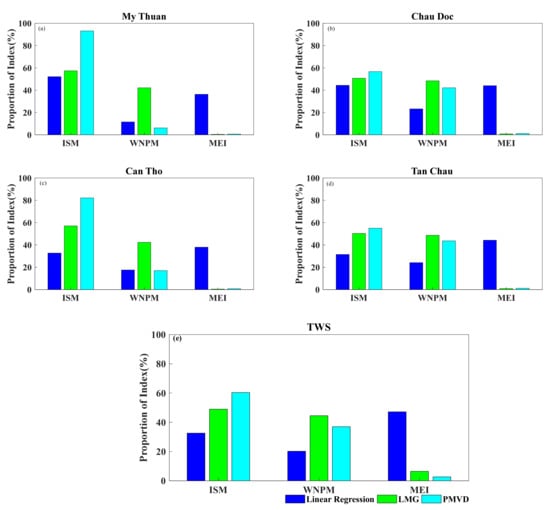
Figure 11.
The resulting proportions of RI for the ISM, WNPM and MEI in the period from 2010 to 2014 for the WL at (a) My Thuan, (b) Chau Doc, (c) Can Tho and (d) Tan Chau, along with (e) those for the TWS.
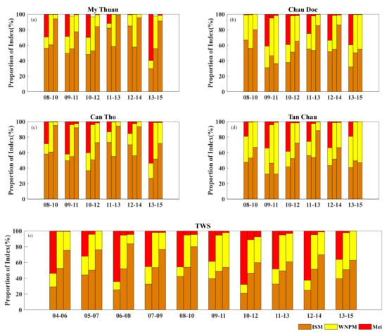
Figure 12.
The temporal changes in the resulting proportions of RI for the ISM, WNPM and MEI for the WL for six three-year time-spans from 2008 to 2015 at (a) My Thuan, (b) Chau Doc, (c) Can Tho and (d) Tan Chau, along with (e) those for the TWS for ten three-year time-spans from 2004 to 2015. Each group of histograms was the result of three methods: linear regression, LMG and PMVD (from left to right).
As shown in Figure 11, the incorporation of the MEI indices into the RI analysis via linear regression resulted in an enlarged RI for the MEI index when compared to that obtained via the LMG and PMVD methods. In terms of the regularity of changes, the results generated from the LMG and PMVD method were similar to those from before. In the results generated from the LMG and PMVD methods, the MEI accounted for a negligible contribution. The reasons for the differences in the methods were described in Section 4.3. The results show that the ENSO effect, represented by the MEI, did play a role in the change in the WL and TWS, although it was relatively weak.
To quantify the influence of the ISM and WNPM on the WL of the Mekong River estuary separately from the influence of ENSO, it was necessary to eliminate the signal of the MEI index in the monsoon index. This was achieved via WTC, as mentioned in Section 3.4. The difference between the results before and after removing ENSO’s influence can be seen as the quantified influence of the ENSO. Taking the WNPM as an example, based on WTC, it is not difficult to see that there was a significant relationship (higher than 0.7) between the WNPM and MEI for the period between 1.8 and 5 years, with a time lag of about 1.5 months, as shown in Figure 13, and the coherence in the period from about 2 years to 3.5 years was the highest, higher than 0.8. It is clear that the WNPM was greatly influenced by the MEI for the period between 1.8 and 5 years, especially at around 2 years and 3.5 years. As a result, the signals for this part were removed.
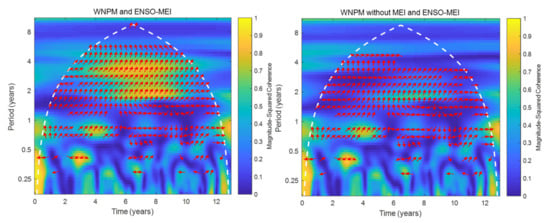
Figure 13.
The coherence between the WNPM and MEI, and the coherence between the MEI and WNPM after the removal of the MEI. The red arrow represents the 5% significance level of high coherence areas, and the phase lag is denoted by the directions (right (left) indicates a phase lag of 0 (180) degrees; up (down) indicates a phase lag of 270 (90) degree).
After removing the signals at the period between 2 and 5 years, the WNPM and MEI no longer showed any obvious coherence in the short-wave signal (Figure 13). Thus, it was considered that the influence of ENSO had been removed from the time series of the monsoon index. The same processing was applied to the ISM time series in order to obtain the time series without ENSO’s influence. The ISM and WNPM indices after the removal of the MEI were utilized to recalculate the proportions of RI of the ISM and WNPM for the WL at the four stations for the period from 2010 to 2014, as shown in Table 6.
Comparing the results after removing ENSO with the original results (Table 6), the following changes could be found: For the proportions of RI of the ISM and WNPM for the WL, the linear regression results enlarged the RI of the ISM at all stations except My Thuan, while the RI resulting from the LMG method was slightly smaller at My Thuan and Can Tho and larger at Chau Doc and Tan Chau. The changes in results for the PMVD method were similar to those at My Thuan and Can Tho, but much larger at Chau Doc and Tan Chau. In addition, the RI of the ISM was higher and the difference between the maximum and minimum was narrower. Compared with those obtained before removing the influence of ENSO, the mean values (ranges) increased (decreased) by 8.78% (14.12%), 2.04% (4.36%) and 14.92% (24.25%), as obtained via multivariate linear regression, LMG and PMVD, respectively. As a result, ENSO can be considered as a potential factor that interferes with results. The influence of the ISM on the water level was more obvious and stable for the monsoon indices after removing the MEI. The influence of the ISM on the TWS increased to 68.79%, 54.60% and 79.43%, as obtained via multivariate linear regression, LMG, and PMVD, respectively. The ISM remained dominant in terms of RI. From 2008 to 2012, after removing the influence of ENSO, the ISM surpassed the WNPM again, rising from 37.81%, 11.94% and 66.77% to 71.81%, 55.63% and 84.19%, as obtained via multivariate linear regression, LMG and PMVD, respectively.
The above results show that the influence of ENSO on the basin-averaged TWS was higher than that on the WL at the estuary. The result is consistent with findings of He et al., (2020) [37]. He et al., (2020) [37] discovered that the ENSO indirectly affected the TWS through the Asian monsoon (including the ISM and WNPM), based on WTC analysis. In addition, the ISM was weakened during ENSO, which was consistent with results from [69,70,71,72]: as El Niño develops in the northern spring, an eastward shift of the Walker circulation over the center of the Pacific occurs, causing the growth of subsidence over South Asia. This suppresses convection over South Asia, leading to a weaker summer monsoon. Though the coherence between ENSO and the WNPM over a long period (e.g., the period between 1.8 and 5 years in Figure 13) has not been previously analyzed, the WNPM has been confirmed to be strengthened during ENSO due to the Pacific negative SST anomalies [73,74,75].
Figure 14 shows the influence of ENSO on the TWS and WL via the rolling data windows. For the WL, the change of results between linear regression and PMVD is more obvious. For the TWS, the RI of the ISM for the TWS increased significantly in the periods from 2008 to 2010 and 2009 to 2011 after the removal of ENSO, whether obtained by linear regression or PMVD. This also coincided with the time of ENSO activity, which happened from 2009 to 2010 [76].
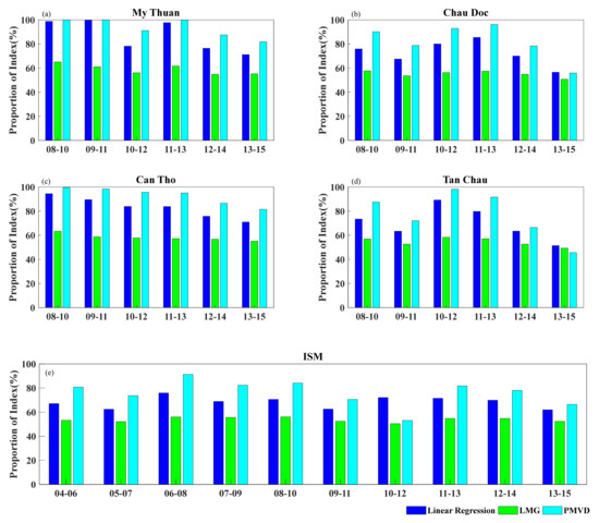
Figure 14.
The temporal changes of the ISM’s effects after ENSO factor removal on the WL for six three-year time-spans from 2008 to 2015 at (a) My Thuan, (b) Chau Doc, (c) Can Tho and (d) Tan Chau, along with (e) those on the TWS for ten three-year time-spans from 2004 to 2015. The changes in the WNPM’s effects were the opposite.
4.5. Future Research and Applications
In this study, after quantifying the contributions of two monsoon indices (i.e., the ISM index and WNPM index) using three RI methods, the ENSO effect was further discussed by introducing the MEI index into the analysis. However, other potential influencing factors (e.g., ocean tides on WL [49,50,77], precipitation and evapotranspiration on TWS) and the restriction of the number of valid factors on RI analysis remain unexplored. Furthermore, we mainly studied the interannual variance (i.e., 3-year and 5-year cycles) of monsoons with regard to the WL and TWS. Nonetheless, for relatively short-term anomalies, such as the performance in drought or flood years in the MRB [4,78], further studies could be conducted in the future.
In addition, other hydrological variables, such as the water discharge [79,80,81], regional precipitation [79,80,81] and evapotranspiration [81,82], could be incorporated into the RI analysis in the form of explanatory or response variables. When combined with the terrestrial water storage [49,83], these hydrological variables should form a terrestrial water balance that allows a more comprehensive analysis. Other regional monsoon or global climate indices can also serve as explanatory variables in this regard. The above proposed elements allow us to extend our methodology and apply it to other large basins with similar geographic configurations and hydroclimatic characteristics as those of the MRB.
5. Conclusions
Aiming at exploring the influences of two monsoons (the Indian summer monsoon (ISM) and western North Pacific monsoon (WNPM)) on the water level (WL) of the Mekong River delta (MRD) and on the terrestrial water storage (TWS) of the entire Mekong River basin (MRB), multivariate linear regression and the Lindeman, Merenda and Gold (LMG) and proportional marginal variance decomposition (PMVD) methods were selected to quantify the relative importance (RI) (or contributions) of the two monsoons. The results showed that the ISM accounts for the majority of the RI for the WL, as well as that for the TWS in the MRD.
Comparing stations closer to (e.g., My Thuan) and farther away from (e.g., Chau Doc) the ocean, the resulting proportions of RI of the ISM for the WL at My Thuan (Chau Doc) station were 81.35% (56.88%), 57.55% (50.94%) and 93.64% (56.84%), as obtained via multivariate linear regression, LMG and PMVD, respectively. This indicates that the WL at stations closer to the ocean is subject more to the influence of the ISM, rendering different results from the three methods. Moreover, the proportions of RI of the ISM for the TWS were 57.55%, 51.64% and 57.99%, as obtained via multivariate linear regression, LMG and PMVD, respectively.
In addition, the same method led to different results using data from different data time-spans, indicating that the RI of the two monsoons’ influences on the WL and TWS varied with time. Considering that climate factors might have caused the fluctuation in the monsoons’ contributions to the WL and TWS, the El Niño–Southern Oscillation (ENSO) index (i.e., the multivariate ENSO index (MEI)) was incorporated into the linear regression analysis. It was found via wavelet transform coherence (WTC) analysis that the MEI presented high correlations with the ISM and WNPM in the periods between 2 and 5 years, highlighting the need for the removal of the ENSO signal from the monsoon indices. Using the ENSO-eliminated data to recalculate the influence of the monsoons on the WL and TWS, the proportions of RI of the ISM for the WL at the four stations were higher while the ranges of change were narrower. The same applied to the TWS. These results indicated that ENSO signals presented a substantial effect on the monsoons. The quantified contributions of influence on the WL for the mean values of four stations (TWS) were 8.78% (11.24%), 2.04% (2.96%) and 14.92% (19.77%), as obtained via multivariate linear regression, LMG and PMVD respectively.
A comparison between the relative importance methods indicated that the linear regression enlarged the existence of the ENSO MEI index compared to the LMG and PMVD methods. This was because linear regression tends to search for the best-fitting result, leading to the enlargement of some variables along with a large deviation in the results. Furthermore, the more balanced results derived from the LMG method demonstrated its comprehensiveness in reflecting the proportions of factors, while the PMVD method focused more on the dominant factor related to the dependent variables. Further improvement could also be possible by including long-period ocean tides (i.e., semiannual and annual tidal constituents) in the analysis. All in all, this study managed to quantify the contributions of two monsoons (the ISM and WNPM) to two hydrological variables (the WL and TWS) in the MRB, which can be generalized to interpret the interactive relations between monsoons and other variables for regions with similar geographic configurations.
Author Contributions
Conceptualization, H.S.F.; methodology, H.S.F. and T.S.; software, T.S.; validation, Z.M., H.S.F. and T.S.; formal analysis, T.S. and H.S.F.; investigation, T.S. and H.S.F.; resources, H.S.F.; data curation, Z.M.; writing—original draft preparation, T.S.; writing—review and editing, T.S., H.S.F. and Z.M.; visualization, T.S.; supervision, H.S.F. and Z.M.; project administration, H.S.F.; funding acquisition, H.S.F. All authors have read and agreed to the published version of the manuscript.
Funding
This study was financially supported by the National Natural Science Foundation of China (NSFC) (Grant No.: 41974003, 41674007, 41374010).
Data Availability Statement
The download links for the water level, monsoon indices, terrestrial water storage and multivariate ENSO Index data are respectively provided in Section 2.1, Section 2.2, Section 2.3 and Section 2.4 within the text.
Acknowledgments
We acknowledge the water level data supplied by the Mekong River Commission (http://www.mrcmekong.org, accessed on 10 July 2020) under agreement and purchased using NSFC Grant No.: 41374010.
Conflicts of Interest
The authors declare no conflict of interest.
References
- Wang, B.; Wu, R.; Lau, K.M. Interannual variability of the Asian summer monsoon: Contrasts between the Indian and the western North Pacific–East Asian monsoons. J. Clim. 2001, 14, 4073–4090. [Google Scholar] [CrossRef]
- Li, J.P.; Zeng, Q.C. A new monsoon index and the geographical distribution of the global monsoons. Adv. Atmos. Sci. 2003, 20, 299–302. [Google Scholar]
- Mahto, S.S.; Mishra, V. Dominance of summer monsoon flash droughts in India. Environ. Res. Lett. 2020, 15, 104061. [Google Scholar] [CrossRef]
- Tang, J.; Cao, H. Drought and flood occurrences in the lancang river basin during the last 60 years: Their variations and teleconnections with monsoons. J. Water Clim. Chang. 2019, 11, 1798–1810. [Google Scholar] [CrossRef]
- Suárez, S.P.; Peiffer, S.; Gebauer, G. Origin and fate of nitrate runoff in an agricultural catchment: Haean, South Korea—Comparison of two extremely different monsoon seasons. Sci. Total Environ. 2019, 648, 66–79. [Google Scholar] [CrossRef] [PubMed]
- Lau, N.-C.; Wang, B. Interactions between the Asian Monsoon and the El Niño/Southern Oscillation; Springer: Singapore, 2006; pp. 479–512. [Google Scholar]
- Shi, J.; Yan, Q.; Yang, Y.; Zhou, F. Possible Modulation of the Interannual ENSO-East Asian Winter Monsoon Relationship by the North American Ice Sheets During the Last 21 ka. Geophys. Res. Lett. 2020, 47, e2020GL089572. [Google Scholar] [CrossRef]
- Wu, R.; Wang, B. A contrast of the East Asian summer monsoon–ENSO relationship between 1962–77 and 1978–93. J. Clim. 2002, 15, 3266–3279. [Google Scholar] [CrossRef]
- Gu, D.; Li, T.; Ji, Z.; Zheng, B. On the Phase Relations between the Western North Pacific, Indian, and Australian Monsoons. J. Clim. 2010, 23, 5572–5589. [Google Scholar] [CrossRef]
- Räsänen, T.A.; Kummu, M. Spatiotemporal influences of ENSO on precipitation and flood pulse in the Mekong River Basin. J. Hydrol. 2013, 476, 154–168. [Google Scholar] [CrossRef]
- Li, S.; He, D. Water level response to hydropower development in the upper Mekong River. Ambio 2008, 37, 170–176. [Google Scholar] [CrossRef]
- Fok, H.S.; He, Q.; Chun, K.P.; Zhou, Z.; Chu, T. Application of ENSO and Drought Indices for Water Level Reconstruction and Prediction: A Case Study in the Lower Mekong River Estuary. Water 2018, 10, 58. [Google Scholar] [CrossRef]
- He, Q.; Fok, H.S.; Chen, Q.; Chun, K.P. Water Level Reconstruction and Prediction Based on Space-Borne Sensors: A Case Study in the Mekong and Yangtze River Basins. Sensors 2018, 18, 3076. [Google Scholar] [CrossRef]
- Johnston, R.; Kummu, M. Water Resource Models in the Mekong Basin: A Review. Water Resour. Manag. 2011, 26, 429–455. [Google Scholar] [CrossRef]
- You, Z.; Feng, Z.M.; Jiang, L.G.; Yang, Y.Z. Population distribution and its spatial relationship with terrain elements in Lancang-Mekong river basin. J. Mt. Res. 2014, 32, 21–29. [Google Scholar]
- Räsänen, T.A.; Koponen, J.; Lauri, H.; Kummu, M. Downstream Hydrological Impacts of Hydropower Development in the Upper Mekong Basin. Water Resour. Manag. 2012, 26, 3495–3513. [Google Scholar] [CrossRef]
- MRC (Mekong River Commission). Overview of the Hydrology of the Mekong Basin; Mekong River Commission: Vientiane, Laos, 2005; Volume 82. [Google Scholar]
- Wang, B. Rainy season of the Asian–Pacific summer monsoon. J. Clim. 2002, 15, 386–398. [Google Scholar] [CrossRef]
- Prathumratana, L.; Sthiannopkao, S.; Kim, K.-W. The relationship of climatic and hydrological parameters to surface water quality in the lower Mekong River. Environ. Int. 2008, 34, 860–866. [Google Scholar] [CrossRef]
- Colin, C.; Siani, G.; Sicre, M.-A.; Liu, Z. Impact of the East Asian monsoon rainfall changes on the erosion of the Mekong River basin over the past 25,000 yr. Mar. Geol. 2010, 271, 84–92. [Google Scholar] [CrossRef]
- Postel, S.L.; Daily, G.C.; Ehrlich, P.R. Human Appropriation of Renewable Fresh Water. Science 1996, 271, 785–788. [Google Scholar] [CrossRef]
- Pauw, K.; Thurlow, J. Economic Losses and Poverty Effects of Droughts and Floods in Malawi. MaSSP Policy Notes 2009. [Google Scholar]
- Zampieri, M.; Carmona Garcia, G.; Dentener, F.; Gumma, M.; Salamon, P.; Seguini, L.; Toreti, A. Surface freshwater limitation explains worst rice production anomaly in India in 2002. Remote Sens. 2018, 10, 244. [Google Scholar] [CrossRef]
- Beven, K.J. Rainfall-Runoff Modelling: The Primer; John Wiley & Sons: Hoboken, NJ, USA, 2012; p. 457. [Google Scholar]
- Tourian, M.J.; Sneeuw, N.; Bárdossy, A. A quantile function approach to discharge estimation from satellite altimetry (EN-VISAT). Water Resour. Res. 2013, 49, 4174–4186. [Google Scholar] [CrossRef]
- Lee, L.; Lawrence, D.; Price, M. Analysis of water-level response to rainfall and implications for recharge pathways in the Chalk aquifer, SE England. J. Hydrol. 2006, 330, 604–620. [Google Scholar] [CrossRef]
- Jiang, T.; Su, B.; Hartmann, H. Temporal and spatial trends of precipitation and river flow in the Yangtze River Basin, 1961–2000. Geomorphology 2007, 85, 143–154. [Google Scholar] [CrossRef]
- Awange, J.L.; Sharifi, M.A.; Ogonda, G.; Wickert, J.; Grafarend, E.W.; Omulo, M.A. The Falling Lake Victoria Water Level: GRACE, TRIMM and CHAMP Satellite Analysis of the Lake Basin. Water Resour. Manag. 2007, 22, 775–796. [Google Scholar] [CrossRef]
- Zheng-Wei, Y.E.; You-Peng, X.U.; Pan, G.B. Precipitation variations and its impact on water level in the lower reaches of jianghuai basin: A case study in the inner lixiahe region. J. Nat. Resour. 2013, 28, 1922–1934. [Google Scholar]
- Das, J.; Jha, S.; Goyal, M.K. On the relationship of climatic and monsoon teleconnections with monthly precipitation over meteorologically homogenous regions in India: Wavelet & global coherence approaches. Atmos. Res. 2020, 238, 104889. [Google Scholar] [CrossRef]
- Yang, P.; Zhan, C.; Xia, J.; Han, J.; Hu, S. Analysis of the spatiotemporal changes in terrestrial water storage anomaly and impacting factors over the typical mountains in China. Int. J. Remote Sens. 2018, 39, 505–524. [Google Scholar] [CrossRef]
- Jin, S.; Zhang, T. Terrestrial Water Storage Anomalies Associated with Drought in Southwestern USA from GPS Observations. Surv. Geophys. 2016, 37, 1139–1156. [Google Scholar] [CrossRef]
- Istanbulluoglu, E.; Wang, T.; Wright, O.M.; Lenters, J. Interpretation of hydrologic trends from a water balance perspective: The role of groundwater storage in the Budyko hypothesis. Water Resour. Res. 2012, 48, 273–279. [Google Scholar] [CrossRef]
- Kim, H.; Yeh, P.J.F.; Oki, T.; Kanae, S. Role of rivers in the seasonal variations of terrestrial water storage over global basins. Geophys. Res. Lett. 2009, 36, L17402. [Google Scholar] [CrossRef]
- Meng, F.; Su, F.; Ying, L.; Kai, T. Changes in terrestrial water storage during 2003–2014 and possible causes in tibetan plateau. J. Geophys. Res. Atmos. 2019, 124, 2909–2931. [Google Scholar] [CrossRef]
- Xu, L.; Chen, N.C.; Zhang, X.; Chen, Z.Q. Spatiotemporal changes in china’s terrestrial water storage from grace satellites and its possible drivers. J. Geophys. Res. Atmos. 2019, 124, 11976–11993. [Google Scholar] [CrossRef]
- He, Q.; Chun, K.P.; Fok, H.S.; Chen, Q.; Dieppois, B.; Massei, N. Water storage redistribution over East China, between 2003 and 2015, driven by intra- and inter-annual climate variability. J. Hydrol. 2020, 583, 124475. [Google Scholar] [CrossRef]
- Long, D.; Shen, Y.; Sun, A.; Hong, Y.; Longuevergne, L.; Yang, Y.; Li, B.; Chen, L. Drought and flood monitoring for a large karst plateau in Southwest China using extended GRACE data. Remote Sens. Environ. 2014, 155, 145–160. [Google Scholar] [CrossRef]
- Ni, S.; Chen, J.; Wilson, C.R.; Li, J.; Hu, X.; Fu, R. Global Terrestrial Water Storage Changes and Connections to ENSO Events. Surv. Geophys. 2018, 39, 1–22. [Google Scholar] [CrossRef]
- Tang, J.; Cheng, H.; Liu, L. Assessing the recent droughts in Southwestern China using satellite gravimetry. Water Resour. Res. 2014, 50, 3030–3038. [Google Scholar] [CrossRef]
- Zhang, Z.; Chao, B.F.; Chen, J.; Wilson, C.R. Terrestrial water storage anomalies of Yangtze River Basin droughts observed by GRACE and connections with ENSO. Glob. Planet. Chang. 2015, 126, 35–45. [Google Scholar] [CrossRef]
- Singh, A.; Seitz, F.; Schwatke, C. Inter-annual water storage changes in the Aral Sea from multi-mission satellite altimetry, optical remote sensing, and GRACE satellite gravimetry. Remote Sens. Environ. 2012, 123, 187–195. [Google Scholar] [CrossRef]
- Frappart, F.; Seyler, F.; Martinez, J.-M.; León, J.G.; Cazenave, A. Floodplain water storage in the Negro River basin estimated from microwave remote sensing of inundation area and water levels. Remote Sens. Environ. 2005, 99, 387–399. [Google Scholar] [CrossRef]
- Zhang, J.; Xu, K.; Yang, Y.; Qi, L.; Hayashi, S.; Watanabe, M. Measuring Water Storage Fluctuations in Lake Dongting, China, by Topex/Poseidon Satellite Altimetry. Environ. Monit. Assess. 2006, 115, 23–37. [Google Scholar] [CrossRef] [PubMed]
- Fok, H.S.; He, Q. Water Level Reconstruction Based on Satellite Gravimetry in the Yangtze River Basin. ISPRS Int. J. Geo-Inf. 2018, 7, 286. [Google Scholar] [CrossRef]
- Achen, C.H. Interpreting and Using Regression; Sage Publications: New York, NY, USA, 1982. [Google Scholar]
- Budescu, D.V. Dominance analysis: A new approach to the problem of relative importance of predictors in multiple regression. Psychol. Bull. 1993, 114, 542–551. [Google Scholar] [CrossRef]
- Johnson, J.W.; LeBreton, J. History and Use of Relative Importance Indices in Organizational Research. Organ. Res. Methods 2004, 7, 238–257. [Google Scholar] [CrossRef]
- Zhou, L.; Fok, H.S.; Ma, Z.; Chen, Q. Upstream Remotely-Sensed Hydrological Variables and Their Standardization for Surface Runoff Reconstruction and Estimation of the Entire Mekong River Basin. Remote Sens. 2019, 11, 1064. [Google Scholar] [CrossRef]
- Shariee, A.M.S.A.; Mohamad, I.N.; Lee, W.K. Backwater Effect of Tidal Water Level Fluctuation and River. In IOP Conference Series: Earth and Environmental Science; IOP Publishing: Bristol, UK, 2020; p. 498. [Google Scholar]
- Wang, B. Reply. Bull. Amer. Meteor. Soc. 2000, 81, 822–824. [Google Scholar] [CrossRef]
- Zhao, Q.; Wu, W.; Wu, Y. Variations in China’s terrestrial water storage over the past decade using GRACE data. Geod. Geodyn. 2015, 6, 187–193. [Google Scholar] [CrossRef]
- Cheng, M.; Tapley, B. Variations in the Earth’s oblateness during the past 28 years. J. Geophys. Res. Space Phys. 2004, 109. [Google Scholar] [CrossRef]
- Swenson, S.; Chambers, D.P.; Wahr, J. Estimating geocenter variations from a combination of GRACE and ocean model output. J. Geophys. Res. Sol. Earth 2008, 113, 08410. [Google Scholar] [CrossRef]
- Ramillien, G.; Frappart, F.; Cazenave, A.; Güntner, A. Time variations of land water storage from an inversion of 2 years of GRACE geoids. Earth Planet. Sci. Lett. 2005, 235, 283–301. [Google Scholar] [CrossRef]
- Swenson, S.; Wahr, J. Post-processing removal of correlated errors in GRACE data. Geophys. Res. Lett. 2006, 33, 1–4. [Google Scholar] [CrossRef]
- Wolter, K.; Timlin, M.S. El Niño/Southern Oscillation behaviour since 1871 as diagnosed in an extended multivariate EN-SO index (MEI. ext). Int. J. Climatol. 2011, 31, 1074–1087. [Google Scholar] [CrossRef]
- Yan, X.; Konopka, P.; Ploeger, F.; Tao, M.; Müller, R.; Santee, M.L.; Bian, J.; Riese, M. El Niño Southern Oscillation influence on the asian summer monsoon anticyclone. Atmos. Chem. Phys. 2018, 18, 8079–8096. [Google Scholar] [CrossRef]
- Menke, W.; Menke, J. Environmental Data Analysis with MatLab; Elsevier: Amsterdam, The Netherlands, 2012. [Google Scholar]
- Gupta, H.V.; Kling, H.; Yilmaz, K.K.; Martinez, G.F. Decomposition of the mean squared error and NSE performance criteria: Implications for improving hydrological modelling. J. Hydrol. 2009, 377, 80–91. [Google Scholar] [CrossRef]
- Groemping, U. Relative Importance for Linear Regression in R: The Package relaimpo. J. Statal Softw. 2006, 17, 925–933. [Google Scholar]
- Grmping, U. Estimators of Relative Importance in Linear Regression Based on Variance Decomposition. Am. Stat. 2007, 61, 139–147. [Google Scholar] [CrossRef]
- Sen, P.K.; Lindeman, R.H.; Merenda, P.F.; Gold, R.Z. Introduction to Bivariate and Multivariate Analysis. J. Am. Stat. Assoc. 1981, 76, 752. [Google Scholar] [CrossRef]
- Feldman, B.E. Relative Importance and Value. SSRN Electron. J. 2005. [Google Scholar] [CrossRef]
- Torrence, C.; Webster, P.J. Interdecadal changes in the ENSO–monsoon system. J. Clim. 1999, 12, 2679–2690. [Google Scholar] [CrossRef]
- Grinsted, A.; Moore, J.; Jevrejeva, S. Application of the cross wavelet transform and wavelet coherence to geophysical time series. Nonlinear Process. Geophys. 2004, 11, 561–566. [Google Scholar] [CrossRef]
- Lachaux, J.P.; Lutz, A.; Rudrauf, D.; Cosmelli, D.; Quyen, M.; Martinerie, J.; Varela, F. Estimating the time-course of coherence between single-trial brain signals: An introduction to wavelet coherence. Neurophysiol. Clin./Clin. Neurophysiol. 2002, 32, 157–174. [Google Scholar] [CrossRef]
- Müller, K.; Lohmann, G.; Neumann, J.; Grigutsch, M.; Mildner, T.; von Cramon, D.Y. Investigating the wavelet coherence phase of the BOLD signal. J. Magn. Reson. Imaging 2004, 20, 145–152. [Google Scholar] [CrossRef]
- Walker, G.T. Correlations in seasonal variations of weather. VIII, A further study of world weather. Mem. Indian Meteorol. Dep. 1924, 24, 275–332. [Google Scholar]
- Rasmusson, E.M.; Carpenter, T.H. The relationship between the Eastern Pacific sea surface temperature and rainfall over India and Sri Lanka. Mon. Weather Rev. 1983, 111, 517–528. [Google Scholar] [CrossRef]
- Webster, P.J.; Yang, S. Monsoon and ENSO: Selectively interactive systems. Q. J. R. Meteor. Soc. 1992, 118, 877–926. [Google Scholar] [CrossRef]
- Ju, J.; Slingo, J.M. The Asian summer monsoon and ENSO. Q. J. R. Meteorol. Soc. 1995, 121, 1133–1168. [Google Scholar] [CrossRef]
- Annamalai, H.; Liu, P. Response of the Asian summer monsoon to changes in El Niño properties. Q. J. R. Meteorol. Soc. 2005, 131, 805–831. [Google Scholar] [CrossRef]
- Minoru, T. Interannual and Interdecadal Variations of the Western North Pacific Monsoon and Baiu Rainfall and their Relationship to the ENSO Cycles. J. Meteorol. Soc. Jpn. 1997, 75, 1109–1123. [Google Scholar]
- Chou, C.; Tu, J.-Y.; Yu, J.-Y. Interannual Variability of the Western North Pacific Summer Monsoon: Differences between ENSO and Non-ENSO Years. J. Clim. 2003, 16, 2275–2287. [Google Scholar] [CrossRef]
- Wijaya, Y.; Hisaki, Y. Differences in the Reaction of North Equatorial Countercurrent to the Developing and Mature Phase of ENSO Events in the Western Pacific Ocean. Climate 2021, 9, 57. [Google Scholar] [CrossRef]
- Peng, H.; Fok, H.; Gong, J.; Wang, L. Improving Stage–Discharge Relation in The Mekong River Estuary by Remotely Sensed Long-Period Ocean Tides. Remote Sens. 2020, 12, 3648. [Google Scholar] [CrossRef]
- Frappart, F.; Bian Ca Maria, S.; Normandin, C.; Blarel, F.; Da Rrozes, J. Influence of recent climatic events on the surface water storage of the tonle sap lake. Sci. Total Environ. 2018, 636, 1520–1533. [Google Scholar] [CrossRef]
- Zhang, J.; Hao, Y.; Hu, B.X.; Huo, X.; Hao, P.; Liu, Z. The effects of monsoons and climate teleconnections on the Niangziguan Karst Spring discharge in North China. Clim. Dyn. 2017, 48, 53–70. [Google Scholar] [CrossRef]
- Ding, Y.; Ye, B.; Han, T.; Shen, Y.; Liu, S. Regional difference of annual precipitation and discharge variation over west China during the last 50 years. Sci. China Ser. D Earth Sci. 2007, 50, 936–945. [Google Scholar] [CrossRef]
- Li, F.; Chen, D.; Tang, Q.; Li, W.; Zhang, X. Hydrological Response of East China to the Variation of East Asian Summer Monsoon. Adv. Meteorol. 2016, 2016, 1–12. [Google Scholar] [CrossRef]
- Zheng, C.; Jia, L.; Hu, G.; Lu, J. Evapotranspiration Estimation in Tropical Monsoon Regions Using Improved ETMonitor Algorithm. In Proceedings of the IGARSS 2019—2019 IEEE International Geoscience and Remote Sensing Symposium, Yokohama, Japan, 28 July–2 August 2019. [Google Scholar]
- Zhang, Y.; Pan, M.; Wood, E.F. On Creating Global Gridded Terrestrial Water Budget Estimates from Satellite Remote Sensing. Surv. Geophys. 2016, 37, 249–268. [Google Scholar] [CrossRef]
Publisher’s Note: MDPI stays neutral with regard to jurisdictional claims in published maps and institutional affiliations. |
© 2021 by the authors. Licensee MDPI, Basel, Switzerland. This article is an open access article distributed under the terms and conditions of the Creative Commons Attribution (CC BY) license (https://creativecommons.org/licenses/by/4.0/).