Review

Hyperspectral and Lidar Data Applied to the Urban Land Cover Machine Learning and Neural-Network-Based Classification: A Review

1
Faculty of Science and Technology, Norwegian University of Life Sciences, 1430 Aas, Norway
2
Helmholtz Center Potsdam, GFZ German Research Centre for Geosciences, Telegrafenberg, 14473 Potsdam, Germany
3
Norwegian Institute of Bioeconomy Research, Raveien 9, 1430 Aas, Norway
*
Author to whom correspondence should be addressed.
Remote Sens. 2021, 13(17), 3393; https://doi.org/10.3390/rs13173393
Submission received: 16 July 2021 / Revised: 17 August 2021 / Accepted: 20 August 2021 / Published: 26 August 2021

Abstract

:
Rapid technological advances in airborne hyperspectral and lidar systems paved the way for using machine learning algorithms to map urban environments. Both hyperspectral and lidar systems can discriminate among many significant urban structures and materials properties, which are not recognizable by applying conventional RGB cameras. In most recent years, the fusion of hyperspectral and lidar sensors has overcome challenges related to the limits of active and passive remote sensing systems, providing promising results in urban land cover classification. This paper presents principles and key features for airborne hyperspectral imaging, lidar, and the fusion of those, as well as applications of these for urban land cover classification. In addition, machine learning and deep learning classification algorithms suitable for classifying individual urban classes such as buildings, vegetation, and roads have been reviewed, focusing on extracted features critical for classification of urban surfaces, transferability, dimensionality, and computational expense.

Graphical Abstract

1. Introduction

Over the last few decades, global urbanization has grown rapidly. By 2050, around 68% of the world’s population will be living in urban areas [1]. This can cause environmental challenges, including ecological problems, poor air quality, deterioration of public health, microclimate changes leading to severe weather, higher temperatures, limited access to water, persistent vulnerability to natural hazards, and the release of toxic particles from fast industrialization into the atmosphere [2,3]. These challenges lead to difficulties in advanced urban analyses due to urban surfaces’ spectral and structural diversity and complexity over a small area [4,5]. Therefore, constant monitoring of urban areas is often highly required. Systematic monitoring and updating of maps are critical in urban areas, where many objects are mobile (vehicles and temporary buildings), and the infrastructure, vegetation, and construction are constantly changing.
Spatiotemporal investigations of the urban regions are today provided by remote sensing technology advances [6]. Especially, airborne remote sensing is a powerful developing tool for urban analysis that offers time-efficient mapping of a city essential for diverse planning [7], management activities [8], and monitoring urban and suburban land uses [9]. It has been proven as a common technique for mapping urban land cover changes to investigate, e.g., social preferences, the regional ecosystem, urbanization change, and biodiversity [10]. Urban remote sensing, in particular, is widely used for the investigation of three-dimensional urban geometry that is crucial for modeling urban morphology [11], identifying various objects, heterogeneous material, and mixtures. However, the growing challenges require a state-of-the-art technological solution in terms of sensors and analysis methods. Continuous development and improvement of remote sensing sensors increase interest in identifying urban land cover types based on spectral, spatial, and structural properties [12,13]. In urban mapping, lidar analyses (light detection and ranging), hyperspectral data (HS), and synthetic aperture radar (SAR) have become significant. Different portions of the electromagnetic spectrum are useful in analyzing urban environments from the reflective spectral range to the microwave radar [14]. The latter provide high-resolution images independent of the time of day and weather; however, due to the requirement of oblique illumination of the scene, occlusion and layover appear, making the analysis of dynamic urban areas difficult [15].
Urban land cover classification accuracy and interpretability based only on a single sensor in complex, dense urban areas are often insufficient [16]. The heterogeneity in the urban areas leads to high spectral variation within one land cover type, resulting in very complex analyses. The impervious surfaces (roofs, parking lots, roads, and pavements) notably vary in the spectral and spatial-structural manner. In addition, scale and spatial resolution are relevant for estimating urban heterogeneity. Scale defines heterogeneity, in which materials are taken into account analytically or absent or grouped into one class, e.g., individual trees, type versus forest, or vegetation in general [17]. Spatial resolution, on the other hand, determines the level of pixel mixing. However, high spatial resolution increases the physical material heterogeneity, increasing the complexity of analyses.
HS data provide spectral information about materials, differentiating them without elevation context. The challenge in the pure spectral analysis is the negligence of object identification, mostly built from various materials maintaining very high intra-object heterogeneity. By contrast, lidar data can distinguish between different land cover classes from the same material at a different height, such as asphaltic open parking lots and roads [18,19]. Furthermore, passive remote sensors, such as HS, are sensitive to atmospheric conditions and illumination, whereas lidar as an active sensor is less sensitive to these factors. This property of lidar enables, e.g., a physical correction of shadow and illumination purposes when combined with HS data [20,21,22,23,24,25] and intensity measurement for urban land cover mapping in shaded areas [26]. Regardless of the spatial and spectral resolution of airborne-based HS sensors, urban environments are characterized by spectral ambiguity and reduced spectral value under the shadow caused by topography changes, buildings, and trees, which can be overcome by adding lidar data as presented by [27]. In order to overcome the limitations of individual sensor capabilities, the recent technologies are based on multisensory fusion in the classification of urban surfaces, combining active and passive remote sensing, such as airborne-based lidar and hyperspectral data (HL-Fusion). Such an HL-Fusion can provide complementary information regarding the three-dimensional topography, spatial structure, and spectral information in the landcover classification purposes [19,28,29,30,31].
Moreover, a fusion of spectral, spatial, and elevation features provides robust and unique information relevant to the urban environment [30]. The airborne HL-Fusion has already been investigated for urban land cover classification purposes [30,32,33]. However, diverse combination methods are implemented on different data and product levels based on either physical or empirical approaches [34]. Furthermore, since all fusion processes are very complex, there is no defined framework for fusing these sensors. Therefore, a comprehensive summary of previous research on data fusion may enhance the understanding of fusion possibilities, challenges, and common issues that limit the classification results in the urban environment.
Machine learning (ML) techniques have been applied as classifiers for HS data [23,24,25,26,27,28]. Depending on the classification aim, different mapping methods are applied to achieve the goal. ML algorithms are in constant improvement, providing algorithms that can hierarchically extract more complex features. This ability is assigned to a subfield of machine learning as deep learning (DL). DL has been proven as an effective technique for feature extraction of HS data on the spatio-spectral level [35,36,37,38,39,40]. Although ML and DL methods are considered relevant classification tools in remote sensing, different algorithms perform best, extracting different pixel- or object-based features. Choosing a classification algorithm for HS data requires knowledge about the features that can be extracted. Especially, DL has gained popularity, thanks to finding unique deep parameters in a pixelwise manner [41]. However, in the urban context, a per pixel classification can lead to noisy results considering high spatial distribution.
Moreover, classification results mainly depend on the number of training samples, limiting the performance and accuracy when the training dataset is insufficient for learning the network algorithm [42]. In order to improve the classification results and reduce the heterogeneity issue, the inclusion of contextual information around pixels and object-oriented classification [43,44] were considered, which allowed retrieving spatial information of HS data and extracting critical spatial patterns of urban land cover classes [45,46]. ML- and DL-based land cover classification in the urban environment from lidar is primarily directed to detect buildings or high vegetation [47]. This is due to the lidar’s ability to extract geometric features from objects, deriving their shape, elevation, and other properties that are useful for a classification purpose. Especially, lidar, in combination with HS, is a powerful tool for classifying urban materials. However, since the objects in the urban scene are complex, analyses with conventional classifiers achieve a low accuracy [48]. Commonly, the application of ML and DL algorithms for classification purposes in the urban environment outperforms traditional classifiers developing very quickly [49].
This review study presents the latest ML and DL urban mapping methods focusing on airborne HS and lidar data. The datasets cover the reflective spectral range of the electromagnetic spectrum (VNIR, SWIR). The paper focuses on ML and DL classification algorithms applied in the urban environment for land cover classes, such as buildings, roads, vegetation, and water analysis. We point out algorithms applicable for HS, lidar, and HL-Fusion and the challenges of applying each algorithm to hyperspectral and lidar data.
The structure of this review paper is arranged as follows (Figure 1): in Section 2, typical urban land cover classes are described in terms of their complexity in HS and lidar data analysis. Section 3 synthesizes the general characteristics of HS and lidar data, highlighting the automated and handcrafted features extracted from both sensors. In Section 4, classification algorithms for urban mapping purposes are described. Section 5 shows the results and discussion of the presented algorithms in urban environment classification. Finally, we point out conclusive remarks on the mapping methods, HL-Fusion potential, perspectives for further research, and recommendations for new research fields.

2. Classified Urban Land Cover Classes

The urban land cover consists of very complex physical materials and surfaces that are constantly having anthropological impacts. The urban surface types are a mosaic of seminatural surfaces such as grass, trees, bare soil, water bodies, and human-made materials of diverse age and composition, such as asphalt, concrete, roof tiles for energy conservation and fire danger [50], and generally impervious surfaces for urban flooding studies and pollution [51]. The complexity of urban analysis also depends on the scale chosen and its purpose. Many classifications refer to urban materials with fine spatial resolution deepening the heterogeneity, allowing a more detailed mapping result. The classification of urban objects, which consist of many different materials and variance within a class, although significant (e.g., in city map updates), becomes a challenge due to the highly nonlinear and heterogeneous composition of different objects surfaces and materials, and thus, there is the need to use more training data for classification purposes, which is time-consuming and computationally expensive.

2.1. Buildings

Buildings in an urban context can be recognized as shapes with planar surfaces and straight lines [52]. Building detection based on remote sensing methods plays a crucial role in many applications in the urban environment, such as in 3D monitoring of urban development in time [53], urban planning, telecommunication network planning, vehicle navigation [33], urban energy planning [53], city management, and damage assessment [54]. Many mapping techniques are based on shape identification, outlines, and preliminary model data [54]. Besides detecting buildings as objects, building roof extraction has recently been a hot topic within the remote sensing community. Building roofs are defined by planarity properties and height derivatives based on elevation. A 3D visualization of buildings is of great importance for infrastructure management and modeling, 3D city mapping, simulations, change detection, and more [55]. Both airborne-based optical and lidar data have been used recently to map buildings. A common way to detect buildings is to use a digital surface model (DSM) [56,57], a normalized DSM (nDSM) [58,59], or a point cloud extracted from lidar data [60,61,62,63]. Lidar is capable of extracting building heights and planar roof faces [33]. It is beneficial for spatiotemporal assessment and investigation of building density for sustainability study and residential development in cities [53].
By contrast, airborne-based HS data can better distinguish between materials at the roof surfaces due to their spectral differences [33]. However, not including the elevation information from the lidar scanner, the classification of buildings and their roofs can be too complex without human expertise. One example is a building surrounded by an arid lawn with open soil, a grass rooftop, a building with an asphaltic parking lot, or bitumen roofing surrounded by asphaltic parking at the building’s ground-level high vegetation (trees) overhanging buildings [64]. Therefore, an HL-Fusion can improve the building classification results offering high accuracy on a spectral and spatial basis.

2.2. Vegetation

Vegetation is recognized by its geometrical complexity, defined by parameters such as the roughness, point density ratio measure [65], and chlorophyll spectral feature. In the last decade, active (Sentinel-1, LiDAR, and radar) and passive (Quickbird, Worldview, Sentinel-2, Landsat, and MODIS) remote sensing has been widely applied to vegetation detection. Lidar data are used to generate virtual 3D tree models [66], map low and high vegetation [67], and, using multispectral lidar, assess vegetation variety regarding its health and density [68], as well as extract vegetation indices, e.g., NDVI [69] for monitoring changes caused by urbanization, anthropogenetic activities, and harvesting applying wavelet transform [70,71]. However, vegetation detection is not a straightforward approach. The analysis is often complex and detailed due to the increasingly finer spatial resolution of remote sensing devices, such as distinguishing photosynthetic and nonphotosynthetic vegetation [72]. Vegetation is often not defined as a whole but as groups, for example, as low vegetation (grass), middle vegetation (shrubs), and high vegetation (trees). One of the more complex challenges is the similar morphology of low/young trees and shrubs, causing misclassification of shrubs as high trees [73]. HS data are also used to detect vegetation on a spectral basis (chlorophyll reflectance), differentiating between vegetation types and healthiness. More biophysical parameters can be defined due to more spectral bands than multispectral lidar (usually 2–3 wavelengths), such as the leaf area index, fractional cover, and foliage biochemistry [74]. Both sensors have been fused in many studies, e.g., for canopy characterization for biomass assessment and estimation of risk of natural hazards [75] and urban tree species mapping [76].

2.3. Roads

Road detection from airborne-based HS and lidar data is essential in remote sensing applications, e.g., a road navigation system, urban planning and management, and geographic information actualization [77,78]. The elevation feature derived from lidar data has been proven as a significant parameter to extract time-efficient road methods compared to optical methods [79]. DSM distinguishes more precise boundaries of surfaces, even in occluded regions [80]. However, only lidar-data-based classification is limited when roads are at the same elevation but made of different materials, such as asphalt, concrete, or other impervious materials [18]. Therefore, HS imaging can differentiate between different materials and their conditions to complement road classification purposes. It has already been proven by Herold et al. [81] for the following uses: map alteration, degradation, and structural damages of road surfaces based on spectral analysis. Usually, to detect roads, texture information is implemented [82]. In addition, lane marks can be used as an indicator for new roads; however, this approach is illumination sensitive [83]. HS data classification without topographic information is challenging when differentiating between two objects made from the same material: differentiation between a parking lot, parking at the ground level, cycleway, and a road [30].

2.4. Miscellaneous

Apart from the above-described land cover classes, the urban environment consists of more complex thematic classes. They commonly cannot be chemically or physically described by a single hyperspectral absorption feature or other single features, such as height or shape, which are, however, extracted from contextual information. Thus, spatial context is critical and necessary for identifying industrial areas, commercial or residential buildings, playgrounds, and harbors in coastal cities. The combination of spectral and spatial features from HS and lidar data shows potential, allowing identifying thematic class and assessing its condition in terms of quality and materials.

3. Key Characteristics of Hyperspectral and Lidar Data

In urban land cover classification, handcrafted feature engineering plays an important role in standard shallow ML algorithms, such as support vector machines (SVM) and random forest (RF). Features are manually derived from remotely sensed data and defined to describe an object of interest, starting from spectral bands through, for example, spectral indices and contextual information, which are generally very useful in defining important biophysical parameters, e.g., for vegetation [84]. However, manually derived features may not sufficiently represent the highly complex and unique urban environment [85]. Depending on the classification objective and classified objects, different features are required. However, in DL, the feature engineering process is simplified as features are extracted during the training step [86]. These automatic high-level features can represent complex spatial correlations and nonlinear relationships. Examples of handcrafted features for both HS and lidar data are described below in this section.

3.1. Hyperspectral (HS) Images

HS data retrieved from an imaging spectrometer are a three-dimensional cube that includes two-dimensional spatial information (x, y) with spectral information at each pixel position xiyj [87]. Each pixel in the obtained digital data contains a nearly continuous spectrum covering the reflective spectral range of the visible, near-infrared (VNIR: 400–1000 nm) and short-wave infrared (SWIR: 1000–2500 nm) [88,89]. HS as a passive system is dependent on the given lighting conditions resulting in high intraclass (within a class) spectral variability. In these wavelength ranges of the electromagnetic spectrum, particular absorption features and shapes make it possible to identify the material’s chemical and physical properties [90]. For example, in urban land cover classification, the reflective spectral range is often used to map diverse soils [91], vegetation [92], rooftop materials [93,94], and other complex physical materials [12,95,96,97].
A high spectral resolution characterizes airborne-based HS applications at the expense of spatial resolution since the HS sensor’s spatial resolution linearly depends on the flight altitude and the instantaneous field of view (IFOW) [98]. However, due to technology development, the spatial resolution of HS is enhanced. Spectrometers with high spectral and spatial resolution have been used to identify detailed urban materials [12,13,94,99]. With a higher spatial resolution of the hyperspectral camera, it is more likely that the spectral signals are less mixed, producing pure pixels and thus detecting materials in the urban environment with high geometric detail and material accuracy. However, a high resolution can lead to difficulties, detecting more diverse materials within a single object, thus increasing heterogeneity and making object-based classification on a coarser scale more challenging. Especially in urban remote sensing, the spatial complexity of the objects and their heterogeneity have been an issue for limited spatial resolution in many studies [94,100]. When within a single pixel, the spectral mixture is very complex, the different spectral properties of individual urban materials are lost, making classification at the level of relevant urban materials challenging [101]. Therefore, a high spatial resolution of hyperspectral sensors has become a crucial parameter in urban mapping.
Land cover classification based on HS data is affected by spatial and spectral resolution, classification purposes (scale and defined land cover classes), mapping methods, and data acquisition and preprocessing. The latter can be the optical geometry, integration time, and other parameters during the acquisition [102]. Especially in airborne-based HS imaging, the sensor experiences altitude variation, which results in geometric distortions in the HS scene [103]. It is always a compromise between off-nadir distortion, spatial resolution, mixed pixels, and SNR (signal-to-noise ratio). Therefore, the strategy and flight scheme must be adapted to the level of the classification target in an advanced way. The flight line’s swath width is reduced at a lower altitude, which requires more flight lines to be flown to cover the target area with changing light conditions due to long integration time [104] and leads to higher off-nadir distortions [105]. However, there are challenges for flying at higher altitudes, such as a high degree of mixed pixels due to a low spatial resolution [106]. In addition, the short integration time at lower altitudes results in lower SNR and decreased sensor sensitivity, producing a more elevated noise floor.

3.1.1. Spectral Features

Within one material, spectral features can vary due to color, coating, degradation, alteration, roughness, the illumination of material, data acquisition, location of the material, and preprocessing data (Figure 2) [97,107,108]. These variations within a material are more and more investigated, generating spectral libraries of complex urban materials [12,109,110] and normalization based on advanced preprocessing. HS images result in high-dimensional data leading to computationally expensive analyses. For this reason, the first common step of the classification process of the HS data is very often a spectral dimensionality reduction to the relevant components applying linear spectral transformations without losing important spectral information [111]. Standard techniques for dimensionality reduction are often statistically based, such as principal component analysis (PCA) [112], linear discriminant analysis (LDA) [113], multivariate curve resolution (MCR) [114], and other unsupervised classification methods. Such data compression saves computing time, reduces noise, and retains needed information [115]. They are often based on the individual image statistic, and thus they are not directly transferable to other flight lines or flight campaigns. In addition, quantification procedures based on the spectral signature are no longer possible. Statistical calculations have been applied to the spectral features of the urban materials, such as continuum removal [116,117]. The continuum-removal algorithm is applied to identify spectral absorption features by their wavelength positions and shapes, removing the overall albedo of the reflectance curve and reducing the searched material’s superimposition [118]. However, the general shape of an absorption feature is relevant for material identification and quantification. Continuum removal may prove effective only for limited studies, excluding the original shape of the spectra. Some handcrafted target-specific features can be calculated from optical remote sensing data, such as normalized difference vegetation index (NDVI) for vegetation detection [8,18,119,120], new impervious index, road detection index, new roof extraction index for the detection of built-up, roads, and roofs [121], normalized difference built-up index [122], visible red and green near-infrared built-up indices [123], road extraction index [124], and hyperspectral difference water index for the detection of urban water bodies [125].

3.1.2. Spatial Information

Spatial-context information is widely used to achieve robust and accurate classification maps considering the neighborhood in the target pixel. While spectral features are the most relevant features in material-based classification, adding spatial features to object classification makes it easier to group pixels with some spectral variance into one class representing an object or land cover type [126] (see Section 3.3). In addition, the spatial noise of the classification results can be reduced [127,128]. In [129], the authors proposed a context-sensitive semisupervised SVM classification technique using contextual information without assumptions about the labeling of contextual pixels. In [130,131], the authors also added the contextual features into hyperspectral image classification, including the information in the classification map generation step. Spatial information is often incorporated in hyperspectral classification problems applying Markov random field where a predefined neighborhood of a pixel assumes that the central pixel belongs to the same class [36,132,133]. Contextual features can also be extracted considering texture (see Section 3.3.1), morphological features (see Section 3.3.2), and image segmentation.

3.2. Lidar Data

Lidar data is a three-dimensional point cloud (x, y, z) which delivers by default information about elevation, multiple-return, the reflected intensity, texture, and waveform-derived feature spaces from the object hit by laser pulse [31,134]. As an active sensor, a lidar system emits radiation from one bandwidth (more in the case of multiwavelength lidar scanners) to the object surface at high repetition rates. Lidar scanners are whiskbroom-type instruments and typically use the monochromatic laser in visible—532 (bathymetric/coastal mapping)—and near-infrared—1064 and 1550 nm—for example, for vegetation detection and differentiation between asphaltic and nonasphaltic roads [135] which can be used as an additional intensity feature in land cover mapping in the reflective spectral range [31]. The advantage of using airborne lidar is insensitivity to relief displacement and illumination conditions [31], retaining full 3D geometry of data.

3.2.1. Height Features and Their Derivatives (HD)

The height feature is used to calculate the three-dimensional coordinates (x,y,z) that generate a gridded 2.5-dimensional topographical profile of the area of interest [31]. Especially in the urban environment, the z value height is crucial for precise contour generation of elevated objects [31]. In addition, the height difference between the lidar return and the lowest point in cylindrical volume has been investigated and proven as an important feature in discriminating ground and nonground points [136,137]. Moreover, a digital surface model (DSM) (Figure 3A) is extracted from the height information applying interpolation of 3D points onto a 2D grid. From a DSM, a surface roughness layer [138] and a normalized DSM (nDSM) (Figure 3C) are calculated, subtracting the digital terrain model (DTM) (Figure 3B) from the DSM [31]. The overlapping of the building height information and the terrain height information is thus excluded. The object representation heterogeneity is therefore reduced, which helps the classification procedure.
The nDSM represents the above-ground points that correspond to the actual heights of the object, omitting information about the objects which could complicate the classification, for example, the differentiation of buildings in lowland or hilly regions. The height information from lidar data helps differentiate between high and low vegetation [139], tree-level characterization applying the canopy height model (CHM) [140], and roads and buildings in the urban environment [8]. In addition, slope calculation (first derivative of any elevation product) and surface curvature (second derivative of the elevation surface) have been applied for detecting surface roughness [141,142] and changes in the normal vectors of the surface [143]. Moreover, calculated skewness and kurtosis models from the lidar elevation data were applied by Antonarakis et al. [144] to determine planted and natural riparian forests and their ages [32]. In the classification approaches, Charaniya et al. [145] included height variation, Bartels and Wei [146] calculated mean variance and standard derivation of the height in the first echo from lidar to measure the roughness, and Im et al. [147] added homogeneity, contrast, and entropy of height as feature spaces after image segmentation (Figure 4).

3.2.2. Intensity Data

Intensity values extracted from lidar data correspond to the peak amplitudes from the illuminated object [31]. Applying intensity as a feature space, Song et al. [148] presented an approach to determine asphalt roads, grass, house roofs, and trees. However, trees’ diverse intensity values undermine the classification due to the canopies’ complex geometry [149]. Moreover, lidar-based intensity can differentiate between low vegetation and impervious surfaces, such as built-up areas. MacFacen et al. [150] applied the estimated mean intensity values from a lidar dataset in an object-based image classification approach. Intensity data are unstable and contain artifacts in the overlapping regions of single strips and eccentricity caused by the gain response, sensor scanning, and environmental factors [151,152,153]. To remove the noise from the intensity data, interpolation, filtering methods, and radiometric calibration are commonly used [148,154]. Additionally, the influence of flying altitude variations, topography, and atmospheric conditions can be corrected, adjusting intensity values, which is called range compensation [155].

3.2.3. Multiple-Return

A lidar-based laser pulse can split into multiple laser returns if it hits a permeable object such as a tree canopy and obtains a response from, e.g., branches, leaves, stems, and the ground [31]. Multiple-return data has been recently used as an additional feature space in the urban mapping in the commercial building, small house, and tree determination [146]. Charaniya et al. [145] and Samadzadegan et al. [48] extracted the first, the last, and the normalized difference (NDI) between these returns to investigate roads and buildings. However, multiple returns occur as well if the laser pulse reaches building edges [156].

3.2.4. Waveform-Derived Features

Full-waveform lidar scanners can retrieve the entire signal of the backscattered laser pulse as a 1D signal profile in the chronological sequence [134,156,157]. A full-waveform lidar system can better correct the intensity values than the discrete systems, such as accurate estimation of the surface slope [158], eliminating the assumption of Lambertian reflectors [159]. However, before using any classification approach, proper radiometric calibration is needed to adjust waveform data from different flight campaigns. Such a radiometric calibration should include preflight, onboard, and vicarious calibration, as presented by Wagner [155]. The waveform-derived features extracted from the gaussian decomposition function have been tested for urban mapping purposes [47,136,160,161]. They include the waveform amplitude, (normalized) number of echoes, their width (Gaussian standard deviation), the difference between the first and the last return, echo shape, and echo cross-section. The latter provides high values for buildings, medium values for vegetation, and low values for roads [137]. For building facades and vegetation that meet multiple echoes, the normalized number of echoes feature is, therefore, relevant [137]. Jutzi and Stilla [162] extracted linear features on roofs based on full-waveform data. Chehata et al. [136] provided that by adding echo width as a feature, the classification results improved for low vegetation. Echo shape was investigated by [137,163], providing low values to roofs and high values to vegetation. It has been proven that the waveform geometry helps to differentiate between trees and built-up areas [136,156,164], determine tree species [165,166], and segment lidar point clouds in an urban area [167]. The waveform amplitude depends on the target. High amplitudes were observed by Chehata et al. [136] for rooftops, gravel, cars, bare soil, and grass, and low amplitudes for asphalt, tar street, and water. Mallet and Bretar [156] observed high amplitudes for grass and bare earth and found that the spread in the pulse and low amplitudes can be assigned to flat surfaces by increasing the incident angle. The echo waveform classification has been applied by Lin and Mills [168] and Doneus et al. [169]. The terrain echoes were separated from echoes from bushes and low vegetation. The echo pulse is wider on the canopy surface and plowed field than on the meadow and street [156]. High point density in full-waveform lidar data helps to detect vegetation types and states [170].

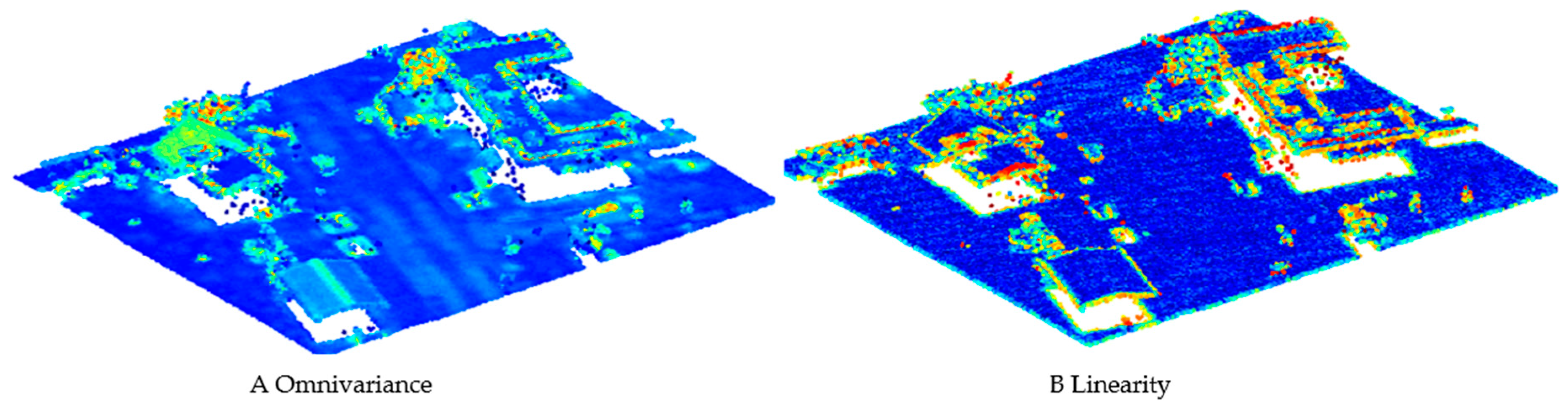
3.2.5. Eigenvalue-Based Features

The eigenvalues are calculated based on the covariance matrix of x, y, and z dimensions of the 3D point cloud as λ1, λ2, and λ3. Eigenvalues as features help detect geometrical parameters, such as plane, edge, and corner [171]. The following structure features have been applied to lidar data: omnivariance, anisotropy, planarity, sphericity, linearity, and eigenentropy for features for context-driven target detection [172] building detection [171]. Some of them are shown in Figure 5. The planarity feature is proven relevant for road classification or other flat surfaces and sphericity for building and natural ground (low vegetation) detection [136].

3.3. Common Features—HS and Lidar

3.3.1. Textural Features

Besides spectral information of hyperspectral sensors, pixel-wise spatial features are relevant for image content, such as textural features. The textural attributes in a hyperspectral scene can be extracted by the local binary patterns (LBP) operator proposed by [173], providing information about the surface granularity [174]. To include spatial information in the classification purposes, the textural operators are window based. Peng et al. [175] extracted them as rotation-invariant features for urban classification purposes except for spectral features and Gabor features [176]. The latter are frequential filters interpreting the texture of the hyperspectral bands used by [177,178]. The texture can be analyzed by applying the gray-level co-occurrence matrix (GLCM) measures [53,179]. GLCM measures, first proposed by Haralick et al. [180], consist of energy, contrast, correlation, entropy, and homogeneity. GLCM dissimilarity, entropy, homogeneity, and second-moment help to detect building edges and height differences. However, contrast, correlation, and variance do not improve building classification and temporal change [53]. Texture features have been used to classify urban materials for pattern recognition in lidar, satellite, and airborne data [48,181,182,183,184]. Samadzadegan et al. [48] calculated four measures: mean, entropy, standard deviation, and homogeneity to classify trees, buildings, and grounds. Huang et al. [181] applied, except for homogeneity and entropy, the angular second moment and dissimilarity from the DSM in the classification approach.

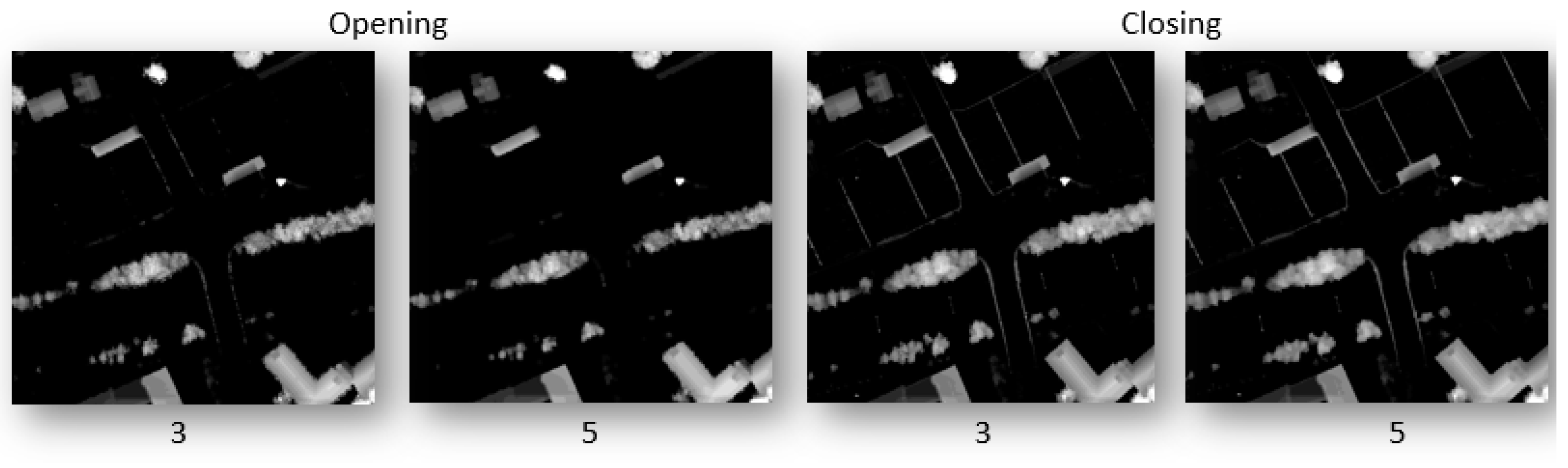
3.3.2. Morphological Features

Mathematical morphology contains operators such as erosion, dilation, opening, closing, rank filters, top hat, and other derived transforms. Mainly, these operators are applied on panchromatic images from hyperspectral sensors, binary or greyscale images with isotropic and geodesic metrics with a structural element [185]. For example, the opening operator focuses on the bright spots, removing objects smaller than the structural element, whereas the closing operator acts on the dark objects (Figure 6). Morphological features with a structural element contain information about the minimum size of the target being investigated [18]. They help reduce shape noise, enhance edges, interpret the texture and extract structures on images regarding their shapes, orientation, and sizes [185,186,187,188]. In image processing, morphological features are based on both spectral and spatial information involving pixels in the neighborhood. They are widely used in hyperspectral image classification [178,187,188,189,190,191], noise reduction in lidar [192], building detection [193], and HL-Fusion-based classification [18]. It has been proven that the inclusion of morphological features improves the accuracy in differentiation between roads and buildings [8].

3.4. Hyperspectral-Lidar Data Fusion

HL-Fusion combines spectral-contextual information obtained by an HS sensor and a lidar scanner’s spectral-spatial-geometrical information. Even if the active and passive sensors characterize different physics, their features can be combined from both sensors. Both sensors cover the reflective spectral range intersecting either in the VIS (532 nm) or the SWIR (1064, 1550 nm) wavelength regions. More rarely, multi-spectral lidar systems are used, which overlap in several of the three common wavelengths, allowing the identification of materials or objects using spectral properties [194]. Under laboratory conditions, prototypical hyperspectral lidar systems are being developed [69,195,196]. The combination of HS and lidar sensors significantly impacts remote sensing, opening up possibilities for fully three-dimensional target analysis [196]. Examples include civil engineering, historical preservation, geomorphological studies, and material processing. However, it is not only the classification concerning 3D geometry determined by sensor fusion. Most rely on geometric simplification of high-dimensional data, reducing both lidar data and HS data to 2.5 grids, where geometrically aligned lidar and HS data are classified based on raster data.
HL-Fusion is usually conducted by adjusting the spatial resolution of one sensor to another (HL to lidar), empirically correcting for geometric errors. Such fusion does not consider the different sensor characteristics (e.g., scan, view, or incidence angles). This kind of fusion also fails when the scene has low-contrast areas, as it is very sensitive to illumination, losing information about details important in complex and heterogeneous urban environments. Despite the dimensional degradation, HL-Fusion has great potential for achieving enhanced results in land cover classification rather than using single sensors, especially when combining spectral and spatial features. In the last decade, fusion has been attempted in this way, for example, by adding to the spectral features extracted from HS data, elevation information, intensity, and other lidar-derived features, which allowed one to upgrade the level of the classification from pixel- to object-based analyses.
Spectral-spatial-based classification on fused data often improves the certainty of a pixel’s belonging to a class. On the other hand, an increasing number of features extracted for classification purposes from different sensors can lead to a curse of dimensionality, especially when the training data are limited [197]. HL-Fusion can also be performed physically, taking into account sensor parameters, measuring principles, quantities, illumination sources, the position of the sensors, and attitude in the preprocessing phase [198,199]. Intensity values can describe the physical link between the spectral and spatial responses of both sensors’ overlapping wavelengths [199]. However, single studies provided HL-Fusion based on fitting spectral data to the first return from lidar data, thus preserving full 3D geometry and structure, improving the scale of analysis and its performance and robustness [200].

4. Classification of Urban Land Cover Classes

Urban land cover classification based on remote sensing data has been carried out on a pixel or object-based classification. Pixel-by-pixel analysis assigns only one of the defined classes to each pixel without considering neighboring pixel decisions [201]. In remote sensing, pixel-based classification relies on the spectral properties of each pixel from the scene. However, pixel-based approaches for high-dimensional remotely sensed HS and lidar data were assumed to be inaccurate for reliable classification purposes [202,203]. Therefore, object-based classification has become relevant, reconstructing reality more truthfully, managing fine spatial resolution data, and suppressing noise. Object-based methods include spatial, textural, contextual, topological, and spectral information [204,205], where objects are defined as classification units [43]. Moreover, the object-based analysis consists of image segmentation, grouping spectrally homogeneous regions, and classification, assigning the segments to the corresponding classes with various properties [206]. Both pixel and object-based classification can be driven in the unsupervised, for example, deep belief networks (DBN) [207,208,209], and stacked autoencoder (SA) [41,210,211,212]) or supervised (RF, SVM) matter.
Analyses on the unsupervised basis separate classification units relying on their common features without providing reference data. This kind of classification is helpful if the knowledge about the study area is limited. In addition, unique classes can be recognized that may have been overlooked applying supervised classification. However, the control over the generated classes is limited, or the final results do not present the analytics intentions, for example, if the desired class is not directly correlated. Supervised classification identifies unknown pixels/objects, validating the accuracy by reference classes assigned to known pixels/objects [213]. One of the advantages of using supervised classification is controlling the number and name of the class labels, which are then assigned to the classification units in the final step [214]. However, supervised classification requires human expertise and the preparation of such reference or ground-truth data adequate for selected area and classification purposes. Such ground-truth sampling includes the removal of outliers and remains representative samples for overall input [215]. This can be accomplished by applying active learning [208,216], random sampling, or stratified random sampling [217].
The ground-truth labeling often requires an equal number of instances assigned to a class. Therefore, a class imbalance issue leads in (multiclass) HS classification to decreased accuracy of many standard algorithms such as decision trees, k-nears neighbor, neural networks, and SVM [218]. Especially for high-dimensional data (HS) and ML/DL-based multiclass problems, the minority classes are neglected or misclassified [219]. Various strategies can be applied to overcome imbalance class issues partially: simplification of the network architecture [38], data augmentation for minority classes, and random sampling for equal class distribution [220].
Complex urban land cover mapping is mainly based on spectral and spatial features of remote sensing data, implemented in classification algorithms. Such an analysis is mainly limited to comparing classification approaches, a general classification scheme, or a small data set, which provides high-accuracy results on local space, excluding generalization and transferability aspects [221]. Often, the evaluation of the classification approach is complicated since the training data may not be representative enough for independent testing data set. In addition, urban land cover analysis usually depends on human expertise at a local scale [84].
Various ML and DL algorithms have been recently explored in feature extraction, pattern recognition, and image classification to deal with high-dimensional space [49,88]. Feature extraction in remote sensing analysis contains mainly shallow supervised and unsupervised and deep feature extraction [222]. In HS data, spectral feature extraction is applied to reduce the high dimensionality and to avoid redundant bands preserving only relevant spectral information. This strategy can also help in increasing separability between different classes. However, spatial feature extraction (texture and morphology) finds the contextual relationship of adjacent pixels improving the only spectral-based classification [132,133,179,209]. In DL, automated extraction of features is common and outperforms shallow ML if the training data fed to the algorithm are not limited.
Aiming to analyze the complexity and improve the DL algorithm learning process quality, a thorough understanding is required of the filter function in the DL architecture [223]. One way to do this is to visualize the parameters of the entire algorithm architecture. However, studies on urban land cover classification based on HS and lidar rarely focus on explaining how the DL algorithms work. As the limited amount of high-dimensional remotely sensed data is fed as input to DL classifiers, there is a probability that the hyperparameter tuning causes overfitting. To avoid this issue, e.g., data augmentation, adding noise, model regularization methods (max-pooling and dropout [224]), and simplifying the model are used. Data augmentation helps diversify training data without new labeling costs, thus leading to more robust classification and adequate classification. In remotely sensed-based classification, training data have been flipped and rotated [225,226], mirrored across horizontal, vertical, and diagonal axes on HS [226,227] and lidar data [228], mixup strategy [229], and generation of virtual training samples through Generative Adversarial Networks (GANs) [230] on HS data. In addition, noise is proven to be suited as a data augmentation type. Haut et al. [231] added random occlusion data augmentation (rectangular figures of different sizes) in various HS image patches. Many studies applied Gaussian white noise during simulation to improve the robustness of the classification and reduce the model’s dependence on local attributes in HL-Fusion [80] and HS data [232].
Apart from overfitting issues, the time-expensive DL algorithms deal with vanishing gradient problems where the learning is unstable and saturates the activations [233]. This problem can be solved by implementing data normalization between each network layer (e.g., local response normalization [234], batch normalization [235], and layer normalization [236]), choosing proper optimizers and nonlinear activation functions [45].
The following section describes the most common ML and DL algorithms for the classification in the urban environment, such as SVM, RF, CNN (convolutional neural network), and RNN (recurrent neural network) (Table 1). Nevertheless, there are many more ML and DL classification algorithms that are not included in this review. Starting with ML algorithms, over time and with technology development, they have become more advanced. Urban analysis with conventional learning-based classifiers was based on interpreting handcrafted low-level features, linear classifiers and nonlinear classifiers, and binary and multiclass classification [88]. Examples are statistical learning on HS data [237], logistic regression on HS data [133], and maximum likelihood classification on lidar data [146]. However, the DL algorithms evolve in classifying urban objects on a larger scale, automatically extracting high-level features. In addition, DL can handle the issue of the complex spatial distribution of spectral information. Automatically derived features in DL rely on a mathematical basis, tuning the model by changing the parameters and neglecting its standard implementations the physical aspect of remote sensing data. In addition to CNNs and RNNs, which have been included in this article, many different DL network frameworks show promising potential for further analysis and a deeper understanding of DL, primarily for HS data. Some of these algorithms are DBN [207,208,209] with SA [41,210,211,212] and GAN [35]. However, these algorithms are in the initial phase of implementation and were not applied until 2019 to HL-Fusion data.

4.1. Support Vector Machines (SVM)

SVM is a supervised ML algorithm that performs the classification of locating a hyperplane between two classes [241]. Such a hyperplane separates two groups in the training dataset, finding the largest margin between the support vectors from different groups [271]. The SVM approach is widely used in pattern recognition, regression, and solving linear equations [271]. It has been proven to be a classifier that can handle the high-dimensional HS data being insensitive to noisy samples [272,273,274,275,276]. Moreover, SVM can deal with smaller training datasets more efficiently than artificial neural networks and maximum likelihood classification algorithms [53]. The decision function of the SVM can be specified by different kernels such as radial basis function (RBF), spectral-based [277], and Gaussian function [19], which classify only in the spectral domain, and composite kernels that include contextual information to the classification [241,278]. The kernel-based methods define the segments by applying the nonlinear geometrical separators [272]. The spectral-based kernel uses the spectral angle of the support vectors to define the hyperplane between them, while for each pixel, spatial information is derived and combined with spectral features in kernel composition. Deep SVM has been implemented with exponential radial basis function, gaussian radial basis function, and neural and polynomial kernel functions, achieving better robustness than conventional classifiers [279].

4.1.1. Buildings

In recent years, a multiwavelength lidar scanner has become an interesting mapping device that can differentiate objects with the same height, such as buildings and trees, based on pseudonormalized difference vegetation index (pseudoNDVI) [68] and geometrical features, e.g., roughness (curvature) [120]. Teo and Wu [15] provided a case study where curvature, intensity, and nDSM were used on multispectral lidar. They applied these lidar features as input for image clustering and found that especially geometric features are suitable for building detection. Huo et al. [8] applied the SVM algorithm with RBF kernel on multispectral lidar data. In the paper, the authors focused, among other things, on building extraction using the combination of nDSM, morphological profiles, novel hierarchical morphological profiles (HMP) [186], pseudoNDVI, and intensity values. Intensity values only extracted from lidar can lead to misclassification of building asphalt roof (parking lot) and a road with similar spectral properties. Shirowzhan and Trinder [53] provided the SVM classification method for building extraction, including DSM, nDSM, and intensity map. However, the results provided a misclassification between roads and buildings in the hilly or vegetation-rich area. A pixel-based classification method is often not able to separate buildings and vegetation boundaries. Samadzadegan et al. [48] proposed a multiclass SVM on building extraction. The authors used first- and last-pulse intensities, first- and last-pulse ranges, entropy, standard deviation, homogeneity, and other geometrical features and showed that texture features improve the final results for building detection. In building analysis based on HS data, the spectral classifie’s domain has limitations in the classification of building roofs (roofing tiles, bitumen, concrete, fiber cement, metals, and slates) [97,238]. To overcome the limitations of single sensor applications, HL-Fusion can complete robust building analysis using spatio-spectral-elevation information. Spectral features from HS data can exclude vegetation growing around and on buildings and differentiate between roof materials. By contrast, lidar data provide shape information that can help determine roof types and building types.

4.1.2. Vegetation

SVM classifier is a standard algorithm in vegetation detection in the urban environment. The authors of [48] suggested a multiclass framework for lidar data, analyzing the normalized difference between the first and the last laser pulse. High vegetation class (trees) was falsely classified as buildings due to limited training data. Teo et al. [120] stated that lidar penetration improves the overall accuracy of vegetation analysis. However, by splitting vegetation into high and low vegetation, lidar data cannot distinguish low height classes such as roads and grass. Huo et al. [8] applied SVM on multispectral lidar data calculating the NDVI and pseudoNDVI [178] and improving the overall classification accuracy, however, having challenges in distinguishing between low and high vegetation. Wang et al. [67] addressed a similar problem in the study and compared single- and dual-wavelength lidar by applying, among others, full-waveform data that were not included in previous studies. The authors showed that dual-wavelength improves the accuracy of low and high vegetation and bare soil and low vegetation compared to single-wavelength lidar. In HS analysis, spectral features are still more accurate in chlorophyll detection than lidar, mainly when a class is characterized by low material variations [40,239]. In addition, HS has been proven to characterize fraction coverage of photosynthetic vegetation, nonphotosynthetic vegetation, and soil [72]. Furthermore, by adding spatial features to the hyperspectral analysis, vegetation detection becomes facilitated [241,242]. Spatial information is also used in HL-Fusion in object-based classification, being able to classify different types of vegetation (tree species) [32,76] and also, in the case of generating hyperspectral point clouds, maintain higher reality factors such as full 3D geometry, generic and robust characteristics [200].

4.1.3. Roads

Huo et al. [8] and Teo et al. [120] applied SVM on multispectral lidar data to detect roads. Achieving high accuracy classification, Huo et al. [8] referred to the misclassification of roads as lawn and bare soil, which can be easily solved by adding HS to the lidar data due to access to more detailed spectral information than lidar only. One of the causes can be similar spectral signatures and insufficient distinctive spectral-spatial features to differentiate between objects. Teo et al. [120] mentioned classification issues applying geometrical features among grass, road, and soil due to similar height. However, spectral features from multiwavelength lidar can overcome the challenge.
In contrast, spectral features in HS analysis applying SVM are often insufficient for achieving robust and accurate results of road classification [40,239]. This is due to considering only spectral information without contextual information and remarkable spectral similarity between physical material belonging to different classes. SVM has also been widely used in road classification on fused HS and lidar data. Brell et al. [200] generated an HS point cloud, where they classified different road materials such as concrete and asphalt. The challenge in distinguishing concrete and asphalt is the influence of shadow deteriorating discrimination between different road materials. The spectral properties of those materials can vary locally based on aging, deterioration, contamination, roughness properties, and other conditions [200].

4.2. Random Forest (RF)

RF is a nonparametric ensemble learning algorithm based on a combination of binary decision tree classifiers [280]. A decision tree in the ensemble is independent of other trees and is trained with random variables by bootstrap sampling [77]. For classification purposes, each tree gives a class prediction as an output. The class that most trees have chosen is considered to be the final result [281]. RF has become a widely used classification algorithm in HS imaging due to its high accuracy and high processing speed [282]. Moreover, RF can handle high-dimensional data selecting redundant spectral bands without overfitting [18,77]. RF has also been applied to airborne-based lidar data as a classifier solving multiclass problems and selecting the essential features for urban mapping [136].

4.2.1. Buildings

Niemeyer et al. [283] proposed a new building classification method based on the 3D point cloud from lidar data. The classification technique transforms the RF classifier into a conditional random field (CRF) framework [218] and provides high-accuracy results for large buildings over 50 m2. However, misclassification occurs at building facades and dormers. In addition, various features derived by lidar have been tested by Chehata et al. [136]. In the paper, multiecho, full-waveform, different height-based, local plane-based, and eigenvalue-based features have been applied to classify buildings. However, confusion errors occurred for transition points between buildings and the ground class.
Further, echo-based features did not have any influence on classification results. Debes et al. [18] presented a fusion framework consisting of unsupervised classification that supports the supervised classification on ensemble learning. They showed that lidar elevation information is required to differentiate between buildings and vegetation or different building types in addition to HS spectral data.

4.2.2. Vegetation

Niemeyer et al. [283] applied an RF classification framework with conditional random fields on lidar data to discriminate vegetation and buildings from each other. Chehata et al. [136] applied RF on lidar data experiencing issues in the classification between vegetation and artificial (roads) and natural ground (grass), respectively. However, applying intensity, height, and texture features of multispectral lidar is very promising for ground-level classes, for example, low vegetation [245]. In HS analysis, spectral features fed to RF classifier provide high vegetation accuracy, good robustness, and insensitivity to noise [244]. Debes et al. [18] chose an RF algorithm on HL-Fusion with elevation features from lidar and NDVI from HS data that outperformed urban area classification [18].

4.2.3. Roads

Niemeyer et al. [283] proposed an RF classification framework for lidar data described in Section 3.1, where one of the classes was asphalt considered a road. However, other objects apart from roads are also made of asphalt, such as roof parking lots, making the analysis difficult, e.g., using only HS data. Jackson et al. [284] mentioned this issue clarifying that the road class pixels are contaminated by other materials and objects such as gravel, puddles, and cars. In addition, vehicles appearing in the image usually have highly reflective properties, making road classification difficult for RF classifiers [8]. Recently, lidar point cloud intensity data have been proposed for road landmark inventory with active learning [285].

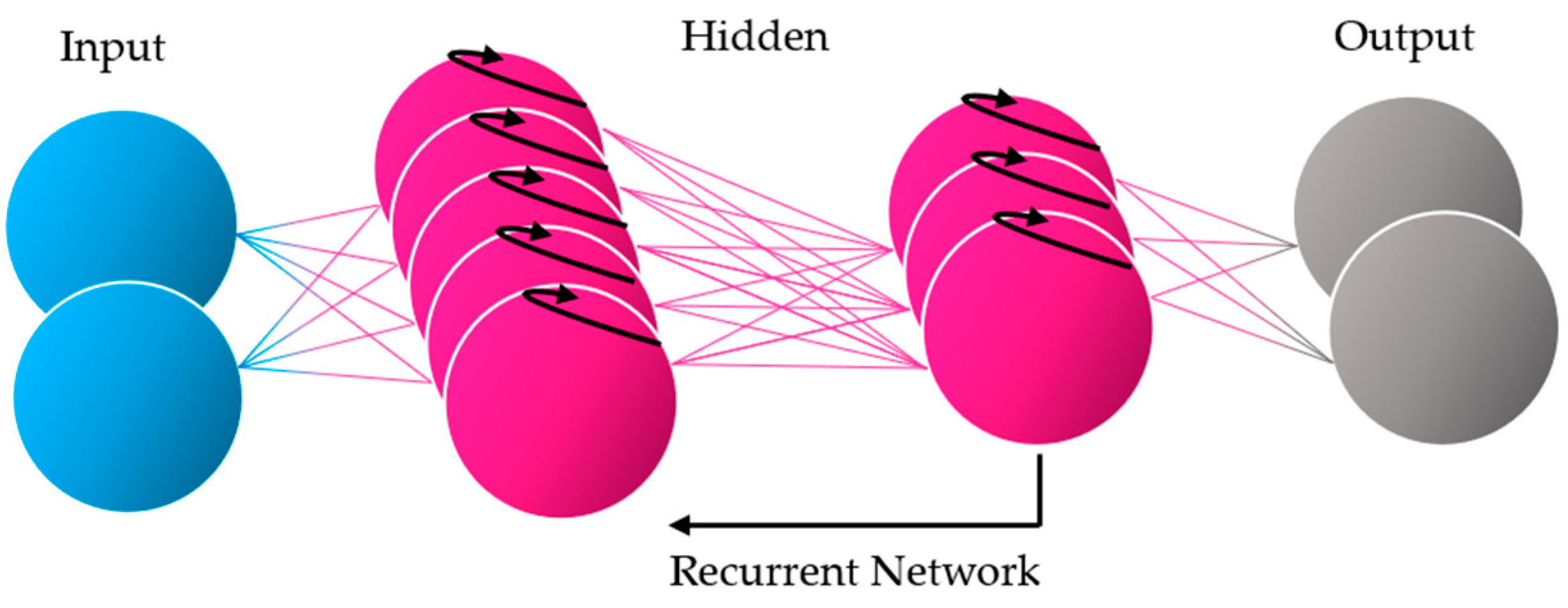
4.3. Convolutional Neural Network (CNN) and Recurrent Neural Network (RNN)

CNN is a DL algorithm that has become an important HS, lidar, and HL-Fusion classification method. The network’s deep convolutional architecture can effectively deal with complex remote sensing data solving nonlinear issues [286] with an example architecture in Figure 7.
CNN has two characteristics different from other DL algorithms, such as local connections and share weights. Local connections help find the data’s spatial relationship, and share weights reduce the number of parameters needed for training purposes and generate a filter [16,286]. CNN architectures can be trained in an unsupervised or supervised way. The unsupervised method is the greedy layer-wise pretraining of hyperspectral data [287,288,289,290]. The supervised method is the standard backpropagation [234,286,291,292]. However, CNNs require a high number of model parameters. The high dimensionality and limited training samples of the remotely sensed data can lead to overfitting and longer processing time than other classification techniques [37,39,293]. An advantage of applying CNN is that the input data must not be preprocessed. CNN is capable of automatically learning abstract features and detecting high-level objects [54]. CNN is used for land cover mapping based on HS data [35,37,38,39] and HL-Fusion [16,30,264,293]. Moreover, CNN has been recently used in combination with other algorithms such as MRF [37] to extract HS pixel vectors on a spatial and spectral basis and extinction profiles [30], capable of effectively reducing noise and improving classification accuracy.
RNN is a DL algorithm widely used to work on sequential data [37]. RNN is a compound of successive recurrent layers capable of extracting contextual parameters at consecutive time steps (Figure 8) [266]. An advantage of RNN is that the input sequences may have different lengths [266]. However, RNN requires a longer processing time than standard ML algorithms, such as SVM or RF [37]. RNN has already been used to extract contextual information of HS data [37,266] and recognize temporal changes of objects measured by the lidar scanner [294].

4.3.1. Buildings

Zhou and Gong [54] focused on building detection in different conditions in damage assessment. Their approach relies on roof object extraction, challenging for lidar data due to sparse points in the boundaries between rooftops and the vertical facades of buildings damaged. In addition, very complex roof configurations cannot be distinguished using lidar data when the training data are too homogeneous. However, DL algorithms such as CNN provided accurate classification results of pre- and post-disaster data with minimal required preprocessing of lidar data and time consumption. Shahajan et al. [55] provided a DL approach that extracts the lidar points from different views assigned to roofs applying height-derived features. However, like the previous study, height-derived features are insufficient in roof type differentiation, and the CNN algorithm requires a large training data set. CNN classifier has also been used in HS data analysis due to its relevant spectral-spatial domain [40]. However, CNN on HS data is time-consuming even if the preprocessing of the fed input is minimized, requires a more extensive data set than shallow ML classifiers, and is not transferable with the same model parameters to other independent test data. Li et al. [30] proposed a DL framework based on spatial and elevation features extracted from extinction profiles, spectral, spatial, and elevation features extracted from the CNN model to classify buildings, among others, on HL-Fusion. Extinction profiles were also used to derive spectral, spatial, and elevation features from HS and lidar data. These features were applied as input for CNN classification on buildings [16]. Morchhale et al. [264] have proven that CNN-based classification on HL-Fusion can distinguish between commercial buildings and highways and between residential buildings and parking lots, improving generalization capability.
Wu et al. [266] introduced deep RNN for HS data classification combining with CNN and creating a convolutional recurrent neural network (CRNN). This framework enabled the extraction of hidden feature representations and provided highly accurate results for building detection. For HS image classification, Mou et al. [37] provided an RNN framework with a GRU activation function that maintains a constant error, helping the network learn more effectively in a high-dimensional space. As a result, his classifier achieved very high accuracy in recognizing commercial and residential areas in the urban environment. Even though only spectral features without contextual information were considered, RNN outperformed standard ML algorithms and CNNs.

4.3.2. Vegetation

CNN is used in HS analysis for vegetation detection [36,39,42,225,239,246,247,248]. Li et al. [246] simultaneously extracted spectro-spatial features of HS data benefitting structural properties needed for detailed vegetation interpretation. However, more and more algorithms for vegetation classification are based on HL-Fusion data. Ghamisi et al., Morchhale et al., and Li et al. [16,30,264] proposed different frameworks based on CNNs. Chen et al. [265] created a CNN framework used to extract the spectral-spatial features of HS data and the elevation features of lidar data. He applied a fully connected DNN to fuse the derived features from both sensors, ending the classification approach with the logistic regression to generate the final classification map [265]. Deep RNN introduced by Mou et al. [37] has been used for vegetation classification. Although RNN resulted in high overall accuracy, the most significant challenges occurred in classifying different grass class types, such as healthy grass, stressed grass, and synthetic grass [37].

4.3.3. Roads

CNN algorithms have already been widely applied as an initial framework for road classification as objects or materials, e.g., gravel, concrete, and asphalt. Santara et al. [38] compared different ML and DL algorithms, including the CNN framework. CNN classified roads as asphalt and gravel with high accuracy only on HS data. Recently, much more often, CNN is used as a classifier for HL-Fusion. Morchhale et al. [264] compared CNN on HS data and HL-Fusion. The classification and differentiation accuracy between road, parking lot, and highway increased in the HL-Fusion. Li et al. [28] proposed that he focuses on classification challenges between similar spectral characteristics of road materials, e.g., asphalt and concrete, and the similar height of different objects, such as grass and asphalt road. Ghamisi et al. [25] applied the CNN classifier with logistic regression and mentioned the challenge of similar spectral signatures of roofs and roads for HS data classification. Wu et al. [266] and Yang et al. [39] proposed CRNNs for HS image classification. Mou et al. [37] presented a different framework—the deep RNN. In both network frameworks, the road was grouped into road and highway. The deep RNN outperformed other conventional classifiers in differentiating similar objects, such as road, highway, and railway [37].

5. Discussion

Airborne HS and lidar data-based classification in the urban environment over the last 20 years has increased significantly since 2016, as shown in the annual number of articles reviewed in this paper found up to 2021 (Figure 9). Therefore, it can be assumed that the interest in HS and lidar remote sensing, advances in sensor technology, computing power, and easy access to remote sensing-based datasets are relevant factors paving the way for large-scale urban environment analysis. However, it has to be noted that the HS-based land cover classification far exceeds lidar and HL-Fusion analyses. Since 2016, the scientific production of urban classification methods based on ML and DL has significantly increased for HS, lidar, and HL-Fusion. This is due to the availability of more advanced computer infrastructures, less expensive sensors with higher resolution, and more accessible data for HS and lidar.
Nevertheless, the HS continued to be widely used. Firstly, this may have been due to the lack of data of the same study area from the two sensors acquired simultaneously. Secondly, most land cover classification approaches are based on physical material classification, which relies significantly on spectral analysis. Sometimes, therefore, it is not necessary to fuse two sensors for some purposes to improve classification by a small fraction with much more effort and time spent fusing the sensors. However, assuming that urban analysis is a highly complex task, one of the fusion application arguments may be that HS and lidar complement each other in spectral and spatial analysis with the addition of elevation information and active and passive sensor characteristics.

5.1. HS-Based Classification

SVM and RF have been proven to be insensitive to noise in HS-based analysis, providing very high accuracy for material classification with limited training data. The only spectral-based SVM classifier can quickly identify object-based classification classes with low material variations. However, for complex urban land cover classification, the spectral domain of the SVM is not sufficient to capture the heterogeneity of the objects or land cover classes built from various materials, for example, identification of impervious and nonvegetated pervious surfaces [238]. For such an analysis, contextual information is necessary. The spatial features can be added to the SVM classifier by applying the composite kernel, improving the accuracy and generalization capabilities.
RF also applies spectral-domain only for HS data. As for SVM, the land cover classes having high material variations within a class are often misclassified, such as road materials (concrete, asphalt, and gravel). The difference and advantage over the SVM classifier is the capability to select important features. This aspect is also advantageous for the DL-based classifiers since shallow ML-based algorithms use handcrafted features controlled and transferred to other independent and unknown test areas.
On the other hand, when the classification objective is focused on a smaller study area, automated features of the DL algorithm may prove to be a better solution for high-dimensional HS data. One factor is that the relationships between objects or land cover classes are not linear in a complex urban environment. By extracting the handcrafted features, we have control and knowledge about them. In contrast, the automated features can obtain high-level features that may allow a much better classification result by recognizing complex relationships that cannot be analyzed by applying shallow ML at the expense of generalizability and transferability. The advantage of the CNN is in its spectral-spatial domain, which searches for high-level features, e.g., by simultaneously extracting spectral and spatial features. As features in CNN are retrieved during the algorithm and the the original, however, normalized, HS data are fed into the model. This saves time for preprocessing, which is necessary for SVM or RF classifiers.
On the other hand, normalization of the extraction of high-level features is notably more time-consuming than classification with shallow ML algorithms. In totally, the increase in dimensions is an enormous challenge in DL classification. The hidden complex relationships are not universally and globally representative. The easiest way to influence this in DL is to ensure the global representativeness of the training and test data which may be hardly possible in remote sensing. Another way is the support of handcrafted features that underrepresent the local properties. In addition, assuming that the algorithm extracts the most important features for correct classification, these features may vary depending on the complexity and diversity of the training data. Therefore, the transferability and generalizability of a model, which is critical, e.g., automatic map updating, is limited. In addition, DL algorithms require a larger training data set, which may not be feasible due to a lack of data and computationally expensive DL algorithms, such as CNN and RNN. The RNN has been proven to outperform even in the spectral domain only compared to standard ML algorithms and CNNs [37]. However, for single classes such as asphalt or concrete-made objects (roads, parking lots, highway), RNN may not solve misclassification only in the spectral domain. The RNN requires more computative time than the CNN, and an extensive training data set is needed. Since RNN considers the temporal domain, this classifier shows greater robustness, transferability, and generalization.

5.2. Lidar-Based Classification

Lidar-based urban land cover classification is not a straightforward approach due to the complexity of the urban environment, where different classifiers with different derived features can identify different land cover classes. Nevertheless, the SVM is a common approach for lidar-based classification. In particular, those land cover classes are distinguished by their unique geometry and where the material composition is not essential. For example, building detection requires the capture of complex geometry, including roofs (planar surfaces) and facades (vertical surfaces). For this purpose, full-waveform data and geometric features are commonly used [243]. However, depending on the specific purpose of the building classification, different features may play an important role. For example, in the analysis of various roof types, the focus was on height-derived features that were insufficient when the roof had a very complex geometry [55]. However, the problem may lie in too low resolution, too sparse point density of the lidar system, or the CNN classifier, which needs a much larger training data set considering heterogeneity and complexity of the objects of interest. In addition, the transition from 3D point cloud to 2.5D representation is challenging to preserve inherent point cloud information.
Raster (2.5D) processing is more efficient in data handling as soon as it comes to spectral-spatial neighborhood analyses and is therefore preferred by most classifiers. The SVM is mainly used for building detection, differentiate between low and high vegetation, and distinguish trees and buildings. The differentiation between low and high vegetation is still a problem. It appears that using height-derived features and full-waveform data from single-wavelength lidar is not sufficient. However, using the same features with a dual-wavelength lidar scanner significantly improved low and high vegetation classification results. Therefore, it can be concluded that spectral features play a significant role in the detailed classification of land cover classes [67]. This assumption of the importance of spectral features in lidar-based classification applying the SVM was also mentioned in a study where spectral features were more critical than geometrical features in classification on a multispectral lidar scanner [120]. In this study, it was found that geometrical features are not able to detect ground-level classes such as roads and grass, which on the other hand, is possible using the spectral features of the multispectral lidar.
Ground-level classes cause many problems also when using full-waveform data. For example, in one study, incorrect classification of grass and sand was caused because the training data contained no balanced classes in the SVM classification [243]. On the other hand, a similar problem of incorrect RF-based classification (this time of low vegetation and roads) also appeared when applying full-waveform data [136]. Therefore, it can be concluded that the last return from lidar is not sufficient for differentiating between ground-level classes. However, this problem has been solved by applying the RF classifier using multispectral lidar data but adding texture features to the elevation and spectral information [245]. However, neither SVM nor RF on single or multispectral lidar can differentiate very heterogeneous classes, such as asphaltic, concrete, or gravel road. This issue can only be solved by adding hyperspectral information on the material using the little available hyperspectral lidar, including reflected intensity information, or integrating lidar with hyperspectral imaging.

5.3. HL-Fusion Classification

HL-Fusion aims to combine the two different sensors with improving the classification result. In urban land cover classification based on HL-Fusion, DL turns out to be the most commonly used method (Table 1). One reason for the DL selection could be the intentional neglect of the more complex preprocessing. Thereby, however, there is a risk of losing transferability and generalizability. This is especially critical for optical data, e.g., if the atmosphere is not corrected according to physical models or the shadow has not been corrected, training data must cover all atmospheric conditions and represent the existing urban heterogeneities. However, both the enormous, rapid development of DL, combined with the progress of sensor technology and multisensory fusion, are becoming an interesting field for further scientific research in the near future. Especially in the analysis of complex urban environments, only a single sensor is usually insufficient for classifying urban land cover classes correctly. Besides material characteristics, spatial correlation is essential and full 3D geometry and topography information. Using context in a more spacious neighborhood for classification purposes, training time increases significantly, especially for DL algorithms (CNN). For shallow ML and DL algorithms, spectral-spatial classification with handcrafted features has been proven to always be more accurate, with the capability of transferability and generalization [16,18,29,264]. HL-Fusion with SVM classifier improved the classification result, but the limited studies did not include the variation between different features derived from HS and lidar. In this case, the application of spectral features from HS and height and derivatives and intensity data proved accurate. Unfortunately, fusing two different sensors also come with some challenges. Adding to the already high-dimensional HS data more dimensions, one can meet the curse of dimensionality problems. By limited training data, high-dimensional feature spaces are often insufficient to recognize desired patterns due to the low ratio of training data to the high dimensional features [295]. More dimensions in source data mean more necessary training and test data due to increased heterogeneity and the number of features, and the need for more computational power and storage.
Although object-based classification is much more comprehensive than pixel-based classification, objects or land cover have become important in classification because they reflect reality much more closely. Spectral features from HS data are reliable for material classification, even in complex urban environments. However, the lack of topographic and geometric information makes accurate results based on only one sensor impossible. Lidar for providing these needed features is very promising in complex urban land cover classification. Lidar complements HS data to add height information to vegetation detection enabling identification of individual trees (full 3D geometry), bushes, low vegetation. In addition, in the detection of the road (edges), lidar provides refined features providing precise boundaries [296]. Thanks to HL-Fusion, there is no need to limit oneself to classify land cover classes, monitor the urbanization processes, and study the urban environment. The potential capabilities of the two sensors enable urban analysis in a holistic, multi-aspect and multidisciplinary way.

6. Conclusions and Future Perspectives

ML and DL revolutionize digital processing of remotely sensed data such as HS, lidar, and HL-Fusion. A significant factor influencing such a great advance in technology is the variety of information obtained time-efficiently by remote sensing systems. Both HS and lidar-based data are used for urban analysis by applying ML and DL algorithms. This review provides the latest information on advances in mapping techniques based on HS and lidar data in urban environments based on the reflective spectral range (400–2500 nm). This multidisciplinary research described in this article was intended to summarize urban land cover classification for ML and DL experts and remote sensing specialists. Particular attention should be paid to DL implementations in HL-Fusion, which may be the key to classifying land cover classes in a complex urban environment. DL is a promising tool for extracting spectral-spatial features and more complex features than classical ML algorithms, which usually improves the accuracy of the classification results. One of the main challenges related to DL’s use is the need for a globally representative dataset for the model training purposes and the availability of annotated lidar data to make it generalizable and transferable: this might require extensive manual work that can be costly but may be overcome applying data augmentation strategy. The HL-Fusion-based classification opens up a new dimension of urban analysis, approximating ML and DL classification results to the reality and going beyond human expertise to discover and care for the urban environment.
The growing trend of using DL in classification will probably remain unchanged over the next few years, discovering new network algorithms, which are already implemented in single case studies. However, as the technology continues to improve, HL-Fusion, despite its high dimensionality, should be considered in analyzing complex urban environments. Crucial is the transferability and generalization aspect, one of the biggest concerns since DLs are usually valid only locally. Inferring from this, it does not allow, for example, the significant updates of city maps.

Author Contributions

Conceptualization, A.K. and M.B.; writing—original draft preparation, A.K.; writing—review and editing, J.R., M.B. and I.B.; supervision, I.B., J.R.; project administration, M.B.; funding acquisition, RFF “Oslo of Akershus Regionale forskningsfond”. All authors have read and agreed to the published version of the manuscript.

Funding

This work is part of the project “FKB maskinlæring” funded by RFF “Oslo og Akershus Regionale forskningsfond”.

Acknowledgments

The authors would like to thank the “FKB maskinlæring” project members for their support and important remarks.

Conflicts of Interest

The authors declare no conflict of interest.

Abbreviations

AbbreviationExplanation
CHMCanopy Height Model
CRFConditional Random Field
CNNConvolutional Neural Network
CRNNConvolutional Recurrent Neural Network
DBNDeep Belief Networks
DLDeep Learning
DSMDigital Surface Model
DTMDigital Terrain Model
GANGenerative Adversarial Network
GLCMGray-Level Co-Occurrence Matrix
HDHeight features and their Derivatives
HSHyperspectral
HL-FusionHyperspectral-Lidar fusion
IFOWInstantaneous Field of View
LidarLight Detection and Ranging
LDALinear Discriminant Analysis
LBPLocal Binary Patterns
MLMachine Learning
MCRMultivariate Curve Resolution
NDINormalized Difference Index
NDVINormalized Difference Vegetation Index
nDSMnormalized Digital Surface Model
PCAPrincipal Component Analysis
psuedoNDVIPseudo Normalized Difference Vegetation Index
RBFRadial Basis Function
RFRandom Forest
RNNRecurrent Neural Network
SARSynthetic Aperture Radar
SWIRShortwave-Infrared
SNRSignal to Noise Ratio
SAStacked Autoencoder
SVMSupport Vector Machines
VNIRVisible and Near-Infrared
VISVisible light

References

  1. United Nations. 2018 Year in Review; United Nations: New York, NY, USA, 2018. [Google Scholar]
  2. Chen, F.; Kusaka, H.; Bornstein, R.; Ching, J.; Grimmond, C.S.B.; Grossman-Clarke, S.; Loridan, T.; Manning, K.W.; Martilli, A.; Miao, S. The integrated WRF/urban modelling system: Development, evaluation, and applications to urban environmental problems. Int. J. Climatol. 2011, 31, 273–288. [Google Scholar] [CrossRef]
  3. Lee, J.H.; Woong, K.B. Characterization of urban stormwater runoff. Water Res. 2000, 34, 1773–1780. [Google Scholar] [CrossRef]
  4. Forster, B.C. Coefficient of variation as a measure of urban spatial attributes, using SPOT HRV and Landsat TM data. Int. J. Remote Sens. 1993, 14, 2403–2409. [Google Scholar] [CrossRef]
  5. Sadler, G.J.; Barnsley, M.J.; Barr, S.L. Information extraction from remotely-sensed images for urban land analysis. In Proceedings of the 2nd European GIS Conference (EGIS’91), Brussels, Belgium, 2–5 April 1991; pp. 955–964. [Google Scholar]
  6. Carlson, T. Applications of remote sensing to urban problems. Remote Sens. Environ. 2003, 86, 273–274. [Google Scholar] [CrossRef]
  7. Coutts, A.M.; Harris, R.J.; Phan, T.; Livesley, S.J.; Williams, N.S.G.; Tapper, N.J. Thermal infrared remote sensing of urban heat: Hotspots, vegetation, and an assessment of techniques for use in urban planning. Remote Sens. Environ. 2016, 186, 637–651. [Google Scholar] [CrossRef]
  8. Huo, L.Z.; Silva, C.A.; Klauberg, C.; Mohan, M.; Zhao, L.J.; Tang, P.; Hudak, A.T. Supervised spatial classification of multispectral LiDAR data in urban areas. PLoS ONE 2018, 13. [Google Scholar] [CrossRef] [PubMed]
  9. Jürgens, C. Urban and suburban growth assessment with remote sensing. In Proceedings of the OICC 7th International Seminar on GIS Applications in Planning and Sustainable Development, Cairo, Egypt, 13–15 February 2001; pp. 13–15. [Google Scholar]
  10. Hepinstall, J.A.; Alberti, M.; Marzluff, J.M. Predicting land cover change and avian community responses in rapidly urbanizing environments. Landsc. Ecol. 2008, 23, 1257–1276. [Google Scholar] [CrossRef]
  11. Batty, M.; Longley, P. Fractal Cities: A Geometry of Form and Function; Academic Press: London, UK; San Diego, CA, USA, 1994. [Google Scholar]
  12. Ben-Dor, E.; Levin, N.; Saaroni, H. A spectral based recognition of the urban environment using the visible and near-infrared spectral region (0.4-1.1 µm). A case study over Tel-Aviv, Israel. Int. J. Remote Sens. 2001, 22, 2193–2218. [Google Scholar] [CrossRef]
  13. Herold, M.; Gardner, M.E.; Roberts, D.A. Spectral resolution requirements for mapping urban areas. IEEE Trans. Geosci. Remote Sens. 2003, 41, 1907–1919. [Google Scholar] [CrossRef] [Green Version]
  14. Brenner, A.R.; Roessing, L. Radar Imaging of Urban Areas by Means of Very High-Resolution SAR and Interferometric SAR. IEEE Trans. Geosci. Remote Sens. 2008, 46, 2971–2982. [Google Scholar] [CrossRef]
  15. Soergel, U. Review of Radar Remote Sensing on Urban Areas. In Radar Remote Sensing of Urban Areas; Soergel, U., Ed.; Springer: Berlin, Germany, 2010; pp. 1–47. [Google Scholar]
  16. Ghamisi, P.; Höfle, B.; Zhu, X.X. Hyperspectral and LiDAR data fusion using extinction profiles and deep convolutional neural network. IEEE J. Sel. Top. Appl. Earth Obs. Remote Sens. 2016, 10. [Google Scholar]
  17. Benz, U.C.; Hofmann, P.; Willhauck, G.; Lingenfelder, I.; Heynen, M. Multi-resolution, object-oriented fuzzy analysis of remote sensing data for GIS-ready information. ISPRS J. Photogramm. Remote Sens. 2004, 58, 239–258. [Google Scholar] [CrossRef]
  18. Debes, C.; Merentitis, A.; Heremans, R.; Hahn, J.; Frangiadakis, N.; Kasteren, T.v.; Liao, W.; Bellens, R.; Pizurica, A.; Gautama, S.; et al. Hyperspectral and LiDAR data fusion: Outcome of the 2013 GRSS data fusion contest. IEEE J. Sel. Top. Appl. Earth Obs. Remote Sens. 2014, 7, 550. [Google Scholar] [CrossRef]
  19. Dalponte, M.; Bruzzone, L.; Gianelle, D. Fusion of hyperspectral and LiDAR remote sensing data for classification of complex forest areas. IEEE Trans. Geosci. Remote Sens. 2008. Available online: https://rslab.disi.unitn.it/papers/R59-TGARS-Dalponte.pdf (accessed on 2 May 2021).
  20. Sohn, H.-G.; Yun, K.-H.; Kim, G.-H.; Park, H.S. Correction of building height effect using LIDAR and GPS. In Proceedings of the International Conference on High Performance Computing and Communications, Sorrento, Italy, 21–23 September 2005; pp. 1087–1095. [Google Scholar]
  21. Guislain, M.; Digne, J.; Chaine, R.; Kudelski, D.; Lefebvre-Albaret, P. Detecting and correcting shadows in urban point clouds and image collections. In Proceedings of the Fourth International Conference on 3D Vision (3DV), Stanford, CA, USA, 25–28 October 2016; pp. 537–545. [Google Scholar]
  22. George, G.E. Cloud Shadow Detection and Removal from Aerial Photo Mosaics Using Light Detection and Ranging (LIDAR) Reflectance Images; The University of Southern Mississippi: Hattiesburg, MS, USA, 2011. [Google Scholar]
  23. Brell, M.; Segl, K.; Guanter, L.; Bookhagen, B. Hyperspectral and Lidar Intensity Data Fusion: A Framework for the Rigorous Correction of Illumination, Anisotropic Effects, and Cross Calibration. IEEE Trans. Geosci. Remote Sens. 2017. Available online: https://www.researchgate.net/publication/313687025_Hyperspectral_and_Lidar_Intensity_Data_Fusion_A_Framework_for_the_Rigorous_Correction_of_Illumination_Anisotropic_Effects_and_Cross_Calibration (accessed on 2 May 2021).
  24. Hui, L.; Di, L.; Xianfeng, H.; Deren, L. Laser intensity used in classification of LiDAR point cloud data. In Proceedings of the International Symposium on Geoscience and Remote Sensing, Boston, MA, USA, 8–11 July 2008. [Google Scholar]
  25. Liu, W.; Yamazaki, F. Object-based shadow extraction and correction of high-resolution optical satellite images. IEEE J. Sel. Top. Appl. Earth Obs. Remote Sens. 2012, 5, 1296–1302. [Google Scholar] [CrossRef]
  26. Zhou, W.; Huang, G.; Troy, A.; Cadenasso, M.L. Object-based land cover classification of shaded areas in high spatial resolution imagery of urban areas: A comparison study. Remote Sens. Environ. 2009, 113, 1769–1777. [Google Scholar] [CrossRef]
  27. Priem, F.; Canters, F. Synergistic use of LiDAR and APEX hyperspectral data for high-resolution urban land cover mapping. Remote Sens. 2016, 8, 787. [Google Scholar] [CrossRef] [Green Version]
  28. Luo, R.; Liao, W.; Zhang, H.; Zgang, L.; Scheunders, P.; Pi, Y.; Philips, W. Fusion of Hyperspectral and LiDAR Data for Classification of Cloud-Shadow Mixed Remote Sensed Scene. IEEE J. Sel. Top. Appl. Earth Obs. Remote Sens. 2017. Available online: https://telin.ugent.be/~wliao/Luo_JSTARS2017.pdf (accessed on 2 May 2021).
  29. Chen, Y.; Li, C.; Ghamisi, P.; Shi, C.; Gu, Y. Deep fusion of hyperspectral and LiDAR data for thematic classification. In Proceedings of the International Geoscience and Remote Sensing Symposium, Beijing, China, 10–14 July 2016. [Google Scholar]
  30. Li, H.; Ghamisi, P.; Soergel, U.; Zhu, X.X. Hyperspectral and LiDAR fusion using deep three-stream convolutional neural networks. Remote Sens. 2018, 10, 1649. [Google Scholar] [CrossRef] [Green Version]
  31. Yan, W.Y.; El-Ashmawy, N.; Shaker, A. Urban land cover classification using airborne LiDAR data: A review. Remote Sens. Environ. 2015. [Google Scholar] [CrossRef]
  32. Alonzo, M.; Bookhagen, B.; Roberts, D.A. Urban tree species mapping using hyperspectral and lidar data fusion. Remote Sens. Environ. 2014, 148, 70–83. [Google Scholar] [CrossRef]
  33. Kokkas, N.; Dowman, I. Fusion of airborne optical and LiDAR data for automated building reconstruction. In Proceedings of the ASPRS Annual Conference, Reno, Nevada, 1–5 May 2006. [Google Scholar]
  34. Torabzadeh, H.; Morsdorf, F.; Schaepman, M.E. Fusion of imaging spectroscopy and airborne laser scanning data for characterization of forest ecosystems. ISPRS J. Photogramm. Remote Sens. 2014, 97, 25–35. [Google Scholar] [CrossRef]
  35. Zhu, L.; Chen, Y.; Ghamisi, P.; Benediktsson, J.A. Generative adversarial networks for hyperspectral image classification. IEEE Trans. Geosci. Remote Sens. 2018, 56, 5046–5063. [Google Scholar] [CrossRef]
  36. Cao, X.; Zhou, F.; Xu, L.; Meng, D.; Xu, Z.; Paisley, J. Hyperspectral image classification with markov random fields and a convolutional neural network. IEEE Trans. Image Process. 2017, 27, 2354–2367. [Google Scholar] [CrossRef] [PubMed] [Green Version]
  37. Mou, L.; Ghamisi, P.; Zhu, X.X. Deep recurrent neural networks for hyperspectral image classification. IEEE Trans. Geosci. Remote Sens. 2017. Available online: https://www.semanticscholar.org/paper/Deep-Recurrent-Neural-Networks-for-Hyperspectral-Mou-Ghamisi/5a391667242b4a631acdd5917681b16a86523987 (accessed on 4 May 2021).
  38. Santara, A.; Mani, K.; Hatwar, P.; Singh, A.; Garg, A.; Padia, K.; Mitra, P. BASS Net: Band-adaptive spectral-spatial feature learning neural network for hyperspectral image classification. IEEE Trans. Geosci. Remote Sens. 2016. Available online: https://arxiv.org/pdf/1612.00144.pdf (accessed on 8 May 2021).
  39. Yang, X.; Li, X.; Lau, R.Y.K.; Zhang, X. Hyperspectral image classification with deep learning models. IEEE Trans. Geosci. Remote Sens. 2018, 99, 1–16. [Google Scholar] [CrossRef]
  40. Li, S.; Song, W.; Fang, L.; Chen, Y.; Ghamisi, P.; Benediktsson, J.A. Deep learning for hyperspectral image classification: An overview. IEEE Trans. Geosci. Remote Sens. 2019, 57, 6690–6709. [Google Scholar] [CrossRef] [Green Version]
  41. Chen, Y.; Lin, Z.; Zhao, X.; Wang, G.; Gu, Y. Deep learning-based classification of hyperspectral data. IEEE J. Sel. Top. Appl. Earth Obs. Remote Sens. 2014, 7, 2094–2107. [Google Scholar] [CrossRef]
  42. Hu, W.; Huang, Y.; Wei, L.; Zhang, F.; Li, H. Deep convolutional neural networks for hyperspectral image classification. J. Sens. 2015. [Google Scholar] [CrossRef] [Green Version]
  43. Yu, Q.; Gong, P.; Clinton, N.; Biging, G.; Kelly, M.; Schirokauer, D. Object-based detailed vegetation classification with airborne high spatial resolution remote sensing imagery. Photogramm. Eng. Remote Sens. 2006, 72, 799–811. [Google Scholar] [CrossRef] [Green Version]
  44. Zhou, W.; Troy, A.; Grove, J.M. Object-based land cover classification and change analysis in the Baltimore metropolian area using multi-temporal high resolution remote sensing data. Sensors 2008, 8, 1613–1636. [Google Scholar] [CrossRef] [Green Version]
  45. Paoletti, M.E.; Haut, J.M.; Plaza, J.; Plaza, A. Deep learning classifiers for hyperspectral imaging: A review. ISPRS J. Photogramm. Remote Sens. 2019, 158, 279–317. [Google Scholar] [CrossRef]
  46. Jiménez, L.O.; Rivera-Medina, J.L.; Rodríguez-Díaz, E.; Arzuaga-Cruz, E.; Ramírez-Vélez, M. Integration of spatial and spectral information by means of unsupervised extraction and classification for homogenous objects applied to multispectral and hyperspectral data. IEEE Trans. Geosci. Remote Sens. 2005, 43, 844–851. [Google Scholar] [CrossRef]
  47. Niemeyer, J.; Wegner, J.; Mallet, C.; Rottensteiner, F.; Soergel, U. Conditional random fields for urban scene classification with full waveform LiDAR data. In Photogrammetric Image Analysis; Stilla, U., Rottensteiner, F., Mayer, H., Jutzi, B., Butenuth, M., Eds.; Springer: Berlin/Heidelberg, Germany, 2011; Volume 6952, pp. 233–244. [Google Scholar]
  48. Samadzadegan, F.; Bigdeli, B.; Ramzi, P. A multiple classifier system for classification of LiDAR remote sensing data using multi-class SVM. In Multiple Classifier Systems; Springer: Berlin/Heidelberg, Germany, 2010; pp. 254–263. [Google Scholar]
  49. Giampouras, P.; Charou, E. Artificial neural network approach for land cover classification of fused hyperspectral and LiDAR data. In Proceedings of the Artificial Intelligence Applications and Innovations, Paphos, Cyprus, 30 September–2 October 2013; pp. 255–261. [Google Scholar]
  50. Medina, M.A. Effects of shingle absorptivity, radiant barrier emissivity, attic ventilation flowrate, and roof slope on the performance of radiant barriers. Int. J. Energy Res. 2000, 24, 665–678. [Google Scholar] [CrossRef]
  51. Ridd, M.K. Exploring a V-I-S-(vegetation—impervious surface-soil) model for urban ecosystem analysis through remote sensing: Comparative anatomy for cities. Int. J. Remote Sens. 1995, 16, 2165–2185. [Google Scholar] [CrossRef]
  52. Haala, N.; Brenner, C. Extraction of buildings and trees in urban environments. ISPRS J. Photogramm. Remote Sens. 1999, 54, 130–137. [Google Scholar] [CrossRef]
  53. Shirowzhan, S.; Trinder, J. Building classification from LiDAR data for spatial-temporal assessment of 3D urban developments. Procedia Eng. 2017, 180, 1453–1461. [Google Scholar] [CrossRef]
  54. Zhou, Z.; Gong, J. Automated residential building detection from airborne LiDAR data with deep neural networks. Adv. Eng. Inform. 2018, 36, 229–241. [Google Scholar] [CrossRef]
  55. Shajahan, D.A.; Nayel, V.; Muthuganapathy, R. Roof classification from 3-D LiDAR point clouds using multiview CNN with self-attention. IEEE Geosci. Remote Sens. Lett. 2019, 99, 1–5. [Google Scholar] [CrossRef]
  56. Matikainen, L.; Hyyppa, J.; Hyyppa, H. Automatic detection of buildings from laser scanner data for map updating. In Proceedings of the International Archives of the Photogrammetry, Remote Sensing and Spatial Information Sciences, Dresden, Germany, 8–10 October 2003. [Google Scholar]
  57. Hug, C.; Wehr, A. Detecting and identifying topographic objects in imaging laser altimetry data. In Proceedings of the International Archives of the Photogrammetry and Remote Sensing, Stuttgart, Germany, 17–19 September 1997; pp. 16–29. [Google Scholar]
  58. Maas, H.G. The potential of height texture measures for the segmentation of airborne laserscanner data. In Proceedings of the 4th International Airborne Remote Sensing Conference and Exhibition and 21st Canadian Symposium on Remote Sensing, Ottawa, ON, Canada, 21–24 June 1999; pp. 154–161. [Google Scholar]
  59. Tóvári, D.; Vögtle, T. Object classifiaction in laserscanning data. Int. Arch. Photogramm. Remote Sens. Spat. Inf. Sci.—ISPRS Arch. 2012, 36. Available online: https://www.researchgate.net/publication/228962142_Object_Classification_in_LaserScanning_Data (accessed on 8 May 2021).
  60. Galvanin, E.A.; Poz, A.P.D. Extraction of building roof contours from LiDAR data using a markov-random-field-based approach. IEEE Trans. Geosci. Remote Sens. 2012, 50, 981–987. [Google Scholar] [CrossRef]
  61. Vosselmann, G. Slope based filtering of laser altimetry data. In Proceedings of the International Archives of the Photogrammetry, Remote Sensing and Spatial Information Sciences, Amsterdam, The Netherlands, 16–22 July 2000; pp. 935–942. [Google Scholar]
  62. Lohmann, P.; Koch, A.; Schaeffer, M. Approaches to the filtering of laser scanner data. In Proceedings of the International Archives of the Photogrammetry, Remote Sensing and Spatial Information Sciences, Amsterdam, The Netherlands, 16–22 July 2000. [Google Scholar]
  63. Tarsha-Kurdi, F.; Landes, T.; Grussenmeyer, P.; Smigiel, E. New approach for automatic detection of buildings in airborne laser scanner data using first echo only. In Proceedings of the ISPRS Commission III Symposium, Photogrammetric Computer Vision, Bonn, Germany, 20–22 September 2006; pp. 25–30. [Google Scholar]
  64. Lodha, S.; Kreps, E.; Helmbold, D.; Fitzpatrick, D. Aerial LiDAR data classification using support vector machines (SVM). In Proceedings of the Third International Symposium on 3D Data Processing, Visualization, and Transmission, Chapel Hill, NC, USA, 14–16 June 2006; pp. 567–574. [Google Scholar]
  65. Rutzinger, M.; Höfle, B.; Pfeifer, N. Detection of high urban vegetation with airborne laser scanning data. In Proceedings of the Forestsat, Montpellier, France, 5–7 November 2007; pp. 1–5. [Google Scholar]
  66. Morsdorf, F.; Nichol, C.; Matthus, T.; Woodhouse, I.H. Assessing forest structural and physiological information content of multi-spectral LiDAR waveforms by radiative transfer modelling. Remote Sens. Environ. 2009, 113, 2152–2163. [Google Scholar] [CrossRef] [Green Version]
  67. Wang, C.K.; Tseng, Y.H.; Chu, H.J. Airborne dual-wavelength LiDAR data for classifying land cover. Remote Sens. 2014, 6, 700–715. [Google Scholar] [CrossRef] [Green Version]
  68. Wichmann, V.; Bremer, M.; Lindenberger, J.; Rutzinger, M.; Georges, C.; Petrini-Monteferri, F. Evaluating the potential of multispectral airborne LiDAR for topographic mapping and land cover classification. In Proceedings of the ISPRS Annals of the Photogrammetry, Remote Sensing and Spatial Information Sciences, La Grande Motte, France, 28 September–3 October 2015. [Google Scholar]
  69. Puttonen, E.; Hakala, T.; Nevalainen, O.; Kaasalainen, S.; Krooks, A.; Karjalainen, M.; Anttila, K. Artificial target detection with a hyperspectral LiDAR over 26-h measurement. Opt. Eng. 2015. Available online: https://www.spiedigitallibrary.org/journals/optical-engineering/volume-54/issue-01/013105/Artificial-target-detection-with-a-hyperspectral-LiDAR-over-26-h/10.1117/1.OE.54.1.013105.full?SSO=1 (accessed on 8 May 2021).
  70. Ghaderpour, E.; Abbes, A.B.; Rhif, M.; Pagiatakis, S.D.; Farah, I.R. Non-stationary and unequally spaced NDVI time series analyses by the LSWAVE software. Int. J. Remote Sens. 2020, 41, 2374–2390. [Google Scholar] [CrossRef]
  71. Martinez, B.; Gilabert, M.A. Vegetation dynamics from NDVI time series analysis using the wavelet transform. Remote Sens. Environ. 2009, 113, 1823–1842. [Google Scholar] [CrossRef]
  72. Okin, G.S. Relative spectral mixture analysis—A multitemporal index of total vegetation cover. Remote Sens. Environ. 2007, 106, 467–479. [Google Scholar] [CrossRef]
  73. Yang, H.; Chen, W.; Qian, T.; Shen, D.; Wang, J. The Extraction of Vegetation Points from LiDAR Using 3D Fractal Dimension Analyses. Remote Sens. 2015, 7, 10815–10831. [Google Scholar] [CrossRef] [Green Version]
  74. Widlowski, J.L.; Pinty, B.; Gobron, N.; Verstraete, M.M. Detection and characterization of boreal coniferous forests from remote sensing data. J. Geophys. Res. 2001, 106, 33405–33419. [Google Scholar] [CrossRef] [Green Version]
  75. Koetz, B.; Sun, G.; Morsdorf, F.; Ranson, K.J.; Kneubühler, M.; Itten, K.; Allgöwer, B. Fusion of imaging spectrometer and LIDAR data over combined radiative transfer models for forest canopy characterization. Remote Sens. Environ. 2007, 106, 449–459. [Google Scholar] [CrossRef]
  76. Dian, Y.; Pang, Y.; Dong, Y.; Li, Z. Urban tree species mapping using airborne LiDAR and hyperspectral data. J. Indian Soc. Remote Sens. 2016, 44, 595–603. [Google Scholar] [CrossRef]
  77. Zhang, Z.; Liu, Q.; Wang, Y. Road extraction by deep residual u-net. IEEE Geosci. Remote Sens. Lett. 2018. Available online: https://arxiv.org/abs/1711.10684 (accessed on 8 May 2021).
  78. Yang, X.; Li, X.; Ye, Y.; Zhang, X.; Zhang, H.; Huang, X.; Zhang, B. Road detection via deep residual dense u-net. In Proceedings of the International Joint Conference on Neural Networks, Budapest, Hungary, 14–19 July 2019. [Google Scholar]
  79. Miliaresis, G.; Kokkas, N. Segmentation and object-based classification for the extraction of the building class from LiDAR DEMs. Comput. Geosci. 2007, 33, 1076–1087. [Google Scholar] [CrossRef]
  80. Zhao, X.; Tao, R.; Li, W.; Li, H.C.; Du, Q.; Liao, W.; Philips, W. Joint Classification of Hyperspectral and LiDAR Data Using Hierarchical Random Walk and Deep CNN Architecture. IEEE Trans. Geosci. Remote Sens. 2020, 58, 7355–7370. [Google Scholar] [CrossRef]
  81. Herold, M.; Roberts, D.; Smadi, O.; Noronha, V. Road condition mapping with hyperspectral remote sensing. In Proceedings of the Airborne Earth Science Workshop, Pasadena, CA, USA, 31 March–2 April 2004. [Google Scholar]
  82. Kong, H.; Audibert, J.Y.; Ponce, J. General Road Detection from a Single Image. IEEE Trans. Image Process. 2010. Available online: https://www.di.ens.fr/willow/pdfs/tip10b.pdf (accessed on 7 May 2021).
  83. Wu, P.C.; Chang, C.Y.; Lin, C. Lane-mark extraction for automobiles under complex conditions. Pattern Recognit. 2014, 47, 2756–2767. [Google Scholar] [CrossRef]
  84. Lin, Y.-C.; Lin, C.; Tsai, M.-D.; Lin, C.-L. Object-based analysis of LiDAR geometric features for vegetation detection in shaded areas. In Proceedings of the XXIII ISPRS Congress, Prague, Czech Republic, 12–19 July 2016. [Google Scholar]
  85. Poux, F.; Hallot, R.P.; Neuville, R.B. Smart point cloud: Definition and remaining challenges. Int. Arch. Photogramm. Remote Sens. Spat. Inf. Sci.—ISPRS Arch. 2016, 42, 119–127. [Google Scholar] [CrossRef] [Green Version]
  86. Arief, H.A.; Strand, G.H.; Tveite, H.; Indahl, U.G. Land cover segmentation of airborne LiDAR data using Stochastic Atrous Network. Remote Sens. 2018, 10, 973. [Google Scholar] [CrossRef] [Green Version]
  87. Clark, R.N. Spectroscopy of rocks and minerals, and principles of spectroscopy. In Manual of Remote Sensing, Remote Sensing for the Earth Sciences; Rencz, A.N., Ed.; John Wiley and Sons: New York, NY, USA, 1999; Volume 3. [Google Scholar]
  88. Signoroni, A.; Savardi, M.; Baronio, A.; Benini, S. Deep learning meets hyperspectral image analysis: A multidisciplinary review. J. Imaging 2019, 5, 52. [Google Scholar] [CrossRef] [Green Version]
  89. Ben-Dor, E. Imaging spectrometry for urban applications. In Imaging Spectrometry; van der Meer, F.D., de Jong, S.M., Eds.; Kluwer Academic Publishers: Amsterdam, The Netherlands, 2001; pp. 243–281. [Google Scholar]
  90. Ortenberg, F. Hyperspectral Sensor Characteristics. In Fundamentals, Sensor Systems, Spectral Libraries, and Data Mining for Vegetation, 2nd ed.; Huete, A., Lyon, J.G., Thenkabail, P.S., Eds.; Hyperspectral remote sensing of vegetation Volume I; CRC Press: Boca Raton, FL, USA, 2011; p. 449. [Google Scholar]
  91. Rossel, R.A.V.; McGlynn, R.N.; McBratney, A.B. Determining the composition of mineral-organic mixes using UV—vis—NIR diffuse reflectance spectroscopy. Geoderma 2006, 137, 70–82. [Google Scholar] [CrossRef]
  92. Adam, E.; Mutanga, O.; Rugege, D. Multispectral and hyperspectral remote sensing for identification and mapping of wetland vegetation:a review. Wetl. Ecol. Manag. 2010, 18, 281–296. [Google Scholar] [CrossRef]
  93. Heiden, U.H.W.; Roessner, S.; Segl, K.; Esch, T.; Mueller, A. Urban structure type characterization using hyperspectral remote sensing and height information. Landsc. Urban. Plan. 2012, 105, 361–375. [Google Scholar] [CrossRef]
  94. Roessner, S.; Segl, K.; Heiden, U.; Kaufmann, H. Automated differentiation of urban surfaces based on airborne hyperspectral imagery. IEEE Trans. Geosci. Remote Sens. 2001, 39, 1525–1532. [Google Scholar] [CrossRef]
  95. Townshend, J.; Justice, C.; Li, W.; Gumey, C.; McManus, J. Global land cover classification by remote sensing: Present capabilities and future possibilities. Remote Sens. Environ. 1991, 35, 243–255. [Google Scholar] [CrossRef]
  96. Heiden, U.; Roessner, S.; Segl, K.; Kaufmann, H. Analysis of Spectral Signatures of Urban Surfaces for their Identification Using Hyperspectral HyMap Data. In Proceedings of the IEEE/ISPRS Joint Workshop on Remote Sensing nd Data Fusion over Urban Areas, Rome, Italy, 8–9 November 2001; pp. 173–177. [Google Scholar]
  97. Heiden, U.; Segl, K.; Roessner, S.; Kaufmann, H. Determination of robust spectral features for identification of urban surface materials in hyperspectral remote sensing data. Remote Sens. Environ. 2007, 111, 537–552. [Google Scholar] [CrossRef] [Green Version]
  98. Meer, F.v.d.; Jong, S.d.; Bakker, W. Imaging Spectrometry: Basic Analytical Techniques. In Imaging Spectrometry; van der Meer, F.D., de Jong, S.M., Eds.; Kluwer Academic Publishers: Dordrecht, The Netherlands, 2001; pp. 17–61. [Google Scholar]
  99. Franke, J.; Roberts, D.A.; Halligan, K.; Menz, G. Hierarchical Multiple Endmember Spectral Mixture Analysis (MESMA) of hyperspectral imagery for urban environments. Remote Sens. Environ. 2009, 113, 1712–1723. [Google Scholar] [CrossRef]
  100. Hepner, G.F.; Housmand, B.; Kulikov, I.; Bryant, N. Investigation of the integration of AVIRIS and IFSAR for urban analysis. Photogramm. Eng. Remote Sens. 1998, 64, 813–820. [Google Scholar]
  101. Linden, S.v.d.; Okujeni, A.; Canters, F.; Degerickx, J.; Heiden, U.; Hostert, P.; Priem, F.; Somers, B.; Thiel, F. Imaging Spectroscopy of Urban Environments. Surv. Geohpys. 2019, 40, 471–488. [Google Scholar] [CrossRef] [Green Version]
  102. Pillay, R.; Picollo, M.; Hardeberg, J.Y.; George, S. Evaluation of the Data Quality from a Round-Robin Test of Hyperspectral Imaging Systems. Sensors 2020, 20, 3812. [Google Scholar] [CrossRef]
  103. Yao, H.; Tian, L.F. Practical methods for geometric distortion correction of aerial hyperspectral imagery. Appl. Eng. Agric. 2004, 20, 367–375. [Google Scholar] [CrossRef]
  104. Lulla, V.; Jensen, R.R. Best Practices for Urban Hyperspectral Remote Sensing Data Acquisition and Processing. In Urban Sustainability: Policy and Praxis; Springer: Berlin/Heidelberg, Germany, 2016; pp. 43–54. [Google Scholar]
  105. Galbraith, A.E.; Theiler, J.; Thome, K.; Ziolkowski, R. Resolution Enhancement of Multilook Imagery for the Multispectral Thermal Imager. IEEE Trans. Geosci. Remote Sens. 2005, 43, 1964–1977. [Google Scholar] [CrossRef]
  106. Pepe, M.; Fregonese, L.; Scaioni, M. Planning airborne photogrammetry and remote-sensing missions with modern platforms and sensors. Eur. J. Remote Sens. 2018, 51, 412–436. [Google Scholar] [CrossRef]
  107. Heiden, U.; Segl, K.; Roessner, S.; Kaufmann, H. Determination and verification of robust spectral features for an automated classification of sealed urban surfaces. In Proceedings of the EARSeL Workshop on Imaging Spectroscopy, Warsaw, Poland, 27–29 April 2005. [Google Scholar]
  108. Lacherade, S.; Miesch, C.; Briottet, X.; Men, H.L. Spectral variability and bidirectional reflectance behavior of urban materials at a 20 cm spatial resolution in the visible and near-infrared wavelength. A case study over Toulouse (France). Int. J. Remote Sens. 2005, 26, 3859–3866. [Google Scholar] [CrossRef]
  109. Herold, M.; Roberts, D.A.; Gardner, M.E.; Dennison, P.E. Spectrometry for urban area remote sensing—Development and analysis of a spectral library from 350 to 2400 nm. Remote Sens. Environ. 2004, 91, 304–319. [Google Scholar] [CrossRef]
  110. Ilehag, R.; Schenk, A.; Huang, Y.; Hinz, S. KLUM: An Urban VNIR and SWIR Spectral Library Consisting of Building Materials. Remote Sens. 2019, 11, 2149. [Google Scholar] [CrossRef] [Green Version]
  111. Manolakis, D.; Lockwood, R.; Cooley, T. Hyperspectral Imaging Remote Sensing: Physics, Sensors, and Algorithms; Cambridge University Press: Cambridge, UK, 2016. [Google Scholar]
  112. Pearson, K. On lines and planes of closest fit to systems of points in space. Philos. Mag. Lett. 1901, 2, 559–572. [Google Scholar] [CrossRef] [Green Version]
  113. Pritchard, J.K.; Stephens, M.; Donnelly, P. Inference of Population Structure Using Multilocus Genotype Data. Genetics 2000, 155, 945–959. [Google Scholar] [CrossRef] [PubMed]
  114. Lawton, W.H.; Sylvestre, E.A. Self modeling curve resolution. Technometrics 1971, 13, 617–633. [Google Scholar] [CrossRef]
  115. Vidal, M.; Amigo, J.M. Pre-processing of hyperspectral images. Essential steps before image analysis. Chemom. Intell. Lab. Syst. 2012, 117, 138–148. [Google Scholar] [CrossRef]
  116. Pandey, D.; Tiwari, K.C. Spectral library creation and analysis of urban built-up surfaces and materials using field spectrometry. Arab. J. Geosci. 2021, 14. [Google Scholar] [CrossRef]
  117. Miller, D.L.; Alonzo, M.; Roberts, D.A.; Tague, C.L.; McFadden, J.P. Drought response of urban trees and turfgrass using airborne imaging spectroscopy. Remote Sens. Environ. 2020, 40. [Google Scholar] [CrossRef]
  118. Clark, R.N.; Swayze, G.A.; Livo, K.E.; Kokaly, R.F.; Sutley, S.H.; Dalton, J.B.; McDougal, R.R.; Gent, C.A. Imaging spectroscopy: Earth and planetary remote sensing with the USGS Tetracorder and expert systems. J. Geophys. Res. 2003, 108. [Google Scholar] [CrossRef]
  119. Yongyang, X.; Liang, W.; Zhong, X.; Zhanlong, C. Building extraction in very high resolution remote sensing imagery using deep learning and guided filters. Remote Sens. 2018, 10. [Google Scholar]
  120. Teo, T.A.; Wu, H.M. Analysis of land cover classification using multi-wavelength LiDAR system. Appl. Sci. 2017, 7, 663. [Google Scholar] [CrossRef] [Green Version]
  121. Pandey, D.; Tiwari, K.C. New spectral indices for detection of urban built-up surfaces and its sub-classes in AVIRIS-NG hyperspectral imagery. Geocarto Int. 2020. [Google Scholar] [CrossRef]
  122. Zha, Y.; Gao, J.; Ni, S. Use of normalized difference built-up index in automatically mapping urban areas from TM imagery. Int. J. Remote Sens. 2003, 24, 583–594. [Google Scholar] [CrossRef]
  123. Estoque, R.C.; Zhang, W.; Tan, K.; Liu, Y.; Liu, S. Multiple classifier system for remote sensing image classification: A review. Sensors 2012, 12, 4764–4792. [Google Scholar]
  124. Shahi, K.; Shafri, H.Z.M.; Taherzadeh, E.; Mansor, S.; Muniandy, R. A novel spectral index to automatically extract road networks from WorldView-2 satellite imagery. Egypt. J. Remote Sens. Space Sci. 2015, 18, 27–33. [Google Scholar] [CrossRef] [Green Version]
  125. Xie, H.; Luo, X.; Xu, X.; Tong, X.; Jin, Y.; Haiyan, P.; Zhou, B. New hyperspectral difference water index for the extraction of urban water bodies by the use of airborne hyperspectral images. J. Appl. Remote Sens. 2014, 8. [Google Scholar] [CrossRef] [Green Version]
  126. Xue, J.; Zhao, Y.; Bu, Y.; Liao, W.; Chan, J.C.-W.; Philips, W. Spatial-Spectral Structured Sparse Low-Rank Representation for Hyperspectral Image Super-Resolution. IEEE Trans. Image Process. 2021, 30, 3084–3097. [Google Scholar] [CrossRef] [PubMed]
  127. Rasti, B.; Scheunders, P.; Ghamisi, P.; Licciardi, G.; Chanussot, J. Noise Reduction in Hyperspectral Imagery: Overview and Application. Remote Sens. 2018, 3, 482. [Google Scholar] [CrossRef] [Green Version]
  128. Gómez-Chova, L.; Alonso, L.; Guanter, L.; Camps-Valls, G.; Calpe, J.; Moreno, J. Correction of systematic spatial noise in push-broom hyperspectral sensors: Application to CHRIS/PROBA images. Appl. Opt. 2008, 47, 46–60. [Google Scholar] [CrossRef] [Green Version]
  129. Bruzzone, L.; Marconcini, M.; Persello, C. Fusion of spectral and spatial information by a novel SVM classification technique. In Proceedings of the IEEE International Geoscience and Remote Sensing Symposium, Barcelona, Spain, 23–27 July 2007. [Google Scholar]
  130. Bovolo, F.; Bruzzone, L. A Context-Sensitive Technique Based on Support Vector Machines for Image Classification. In Proceedings of the International Conference on Pattern Recognition and Machine Intelligence, Kolkata, India, 20–22 December 2005; pp. 260–265. [Google Scholar]
  131. Farag, A.A.; Mohamed, R.H.; El-Baz, A. A unified framework for MAP estimation in remote sensing image segmentation. IEEE Trans. Geosci. Remote Sens. 2005, 43, 1617–1634. [Google Scholar] [CrossRef]
  132. Sun, L.; Wu, Z.; Liu, J.; Xiao, L.; Wei, Z. Supervised spectral-spatial hyperspectral image classification with weighted Markov Random Fields. IEEE Trans. Geosci. Remote Sens. 2015, 53, 1490–1503. [Google Scholar] [CrossRef]
  133. Li, J.; Bioucas-Dias, J.M.; Plaza, A. Spectral-spatial hyperspectral image segmentation using subspace multinomial logistic regression and markov random fields. IEEE Trans. Geosci. Remote Sens. 2012, 50. [Google Scholar] [CrossRef]
  134. Wehr, A.; Lohr, U. Airborne laser scanning—An introduction and overview. ISPRS J. Photogramm. Remote Sens. 1999, 54, 68–82. [Google Scholar] [CrossRef]
  135. Clode, S.; Rottensteiner, F.; Kootsookos, P.; Zelniker, E. Detection and vectorization of roads from LiDAR data. Photogramm. Eng. Remote Sens. 2007, 73, 517–535. [Google Scholar] [CrossRef] [Green Version]
  136. Chehata, N.; Guo, L.; Mallet, C. Airborne LiDAR feature selection for urban classification using random forests. Laserscanning 2009, 38. [Google Scholar]
  137. Guo, L.; Chehata, N.; Mallet, C.; Boukir, S. Relevance of airborne LiDAR and multispectral image data for urban scene classification using random forests. ISPRS J. Photogramm. Remote Sens. 2011, 66, 56–66. [Google Scholar] [CrossRef]
  138. Priestnall, G.; Jaafar, J.; Duncan, A. Extracting urban features from LiDAR digital surface models. Comput. Environ. Urban. Syst. 2000, 24, 65–78. [Google Scholar] [CrossRef]
  139. Hecht, R.; Meinel, G.; Buchroithner, M.F. Estimation of urban green volume based on single-pulse LiDAR data. IEEE Trans. Geosci. Remote Sens. 2008, 46. [Google Scholar] [CrossRef]
  140. Alonso, L.; Picos, J.; Bastos, G.; Armesto, J. Detection of Very Small Tree Plantations and Tree-Level Characterization Using Open-Access Remote-Sensing Databases. Remote Sens. 2020, 12, 2276. [Google Scholar] [CrossRef]
  141. Grohmann, C.H.; Smith, M.J.; Riccomini, C. Muli-scale Analysis of Topographic Surface Roughness in the Midland Valley, Scotland. IEEE Trans. Geosci. Remote Sens. 2011, 49, 1200–1213. [Google Scholar] [CrossRef] [Green Version]
  142. Brubaker, K.M.; Myers, W.L.; Drohan, P.J.; Miller, D.A.; Boyer, E.W. The Use of LiDAR Terrain Data in Characterizing Surface Roughness and Microtopography. Appl. Environ. Soil Sci. 2013, 2013. [Google Scholar] [CrossRef]
  143. Brenner, C. Dreidimensionale Gebäuderekonstruktion aus digitalen Oberflächenmodellen und Grundrissen. Ph.D. Thesis, Stuttgart University, Stuttgart, Germany, 2000. [Google Scholar]
  144. Antonarakis, A.S.; Richards, K.S.; Brasington, J. Object-based land cover classification using airborne LiDAR. Remote Sens. Environ. 2008, 112, 2988–2998. [Google Scholar] [CrossRef]
  145. Charaniya, A.P.; Manduchi, R.; Lodha, S.K. Supervised parametric classification of aerial LiDAR data. In Proceedings of the IEEE Computer Society Conference on Computer Vision and Pattern Recognition Workshops, Washington, DC, USA, 27 June–2 July 2004. [Google Scholar]
  146. Bartels, M.; Wei, H. Maximum likelihood classification of LiDAR data incorporating multiple co-registered band. In Proceedings of the 4th International Workshop on Pattern Recognition in Remote Sensing in conjunction with the 18th International Conference on Pattern Recognition, Hong Kong, 20–24 August 2006. [Google Scholar]
  147. Im, J.; Jensen, J.R.; Hodgson, M.E. Object-based land cover classification using high-posting-density LiDAR data. GIsci. Remote Sens. 2008, 45, 209–228. [Google Scholar] [CrossRef] [Green Version]
  148. Song, J.H.; Han, S.H.; Yu, K.Y.; Kim, Y.I. Assessing the possibility of land-cover classification using LiDAR intensity data. Int. Arch. Photogramm. Remote Sens. Spat. Inf. Sci. ISPRS Arch. 2002, 34, 259–262. [Google Scholar]
  149. Yoon, J.-S.; Lee, J.-I. Land cover characteristics of airborne LiDAR intensity data: A case study. IEEE Geosci. Remote Sens. Lett. 2008, 5, 801–805. [Google Scholar] [CrossRef]
  150. MacFaden, S.W.; O´Neil-Dunne, J.P.M.; Royar, A.R.; Lu, J.W.T.; Rundle, A.G. High-resolution tree canopy mapping for New York City using LiDAR and object-based image analysis. J. Appl. Remote Sens. 2012, 6. [Google Scholar] [CrossRef]
  151. Yan, W.Y.; Shaker, A. Reduction of striping noise in overlapping LiDAR intensity data by radiometric normalization. In Proceedings of the XXIII ISPRS Congress, Prague, Czech Republic, 12–19 July 2016. [Google Scholar]
  152. Nobrega, R.A.A.; Quintanilha, J.A.; O´Hara, C.G. A noise-removal approach for LiDAR intensity images using anisotropic diffusion filtering to preserve object shape characteristics. In Proceedings of the ASPRS Annual Conference, Tampa, FL, USA, 7–11 May 2007. [Google Scholar]
  153. Minh, N.Q.; Hien, L.P. Land cover classification using LiDAR intensity data and neural network. J. Korean Soc. Surv. Geodesy Photogramm. Cartogr. 2011, 29.4, 429–438. [Google Scholar] [CrossRef]
  154. Brennan, R.; Webster, T.L. Object-oriented land cover classification of LiDAR-derived surfaces. Can. J. Remote Sens. 2006, 32, 162–172. [Google Scholar] [CrossRef]
  155. Wagner, W. Radiometric calibration of small-footprint full-waveform airborne laser scanner measurements: Basic physical concepts. ISPRS J. Photogramm. Remote Sens. 2010, 65, 505–513. [Google Scholar] [CrossRef]
  156. Mallet, C.; Bretar, F. Full-waveform topographic LiDAR: State-of-the-art. ISPRS J. Photogramm. Remote Sens. 2009, 64, 1–16. [Google Scholar] [CrossRef]
  157. Bretar, F.; Chauve, A.; Mallet, C.; Jutzi, B. Managing full waveform LiDAR data: A challenging task for the forthcoming years. Int. Arch. Photogramm. Remote Sens. Spat. Inf. Sci. ISPRS Arch. 2008, XXXVII, 415–420. [Google Scholar]
  158. Kirchhof, M.; Jutzi, B.; Stilla, U. Iterative processing of laser scanning data by full waveform analysis. ISPRS J. Photogramm. Remote Sens. 2008, 63, 99–114. [Google Scholar] [CrossRef]
  159. Höfle, B.; Pfeifer, N. Correction of laser scanning intensity data: Data and model-driven approaches. ISPRS J. Photogramm. Remote Sens. 2007, 62, 1415–1433. [Google Scholar] [CrossRef]
  160. Alexander, C.; Tansey, K.; Kaduk, J.; Holland, D.; Tate, N.J. Backscatter coefficient as an attribute for the classification of full-waveform airborne laser scanning data in urban areas. ISPRS J. Photogramm. Remote Sens. 2010, 65, 423–432. [Google Scholar] [CrossRef] [Green Version]
  161. Neuenschwander, A.L.; Magruder, L.A.; Tyler, M. Landcover classification of small-footprint, full-waveform LiDAR data. J. Appl. Remote Sens. 2009, 3. [Google Scholar] [CrossRef]
  162. Jutzi, B.; Stilla, U. Waveform processing of laser pulses for reconstruction of surfacer in urban areas. Meas. Tech. 2005. Available online: https://www.researchgate.net/publication/43136634_Waveform_processing_of_laser_pulses_for_reconstruction_of_surfaces_in_urban_areas (accessed on 2 May 2021).
  163. Chauve, A.; Mallet, C.; Bretar, F.; Durrieu, S.; Pierrot-Deseilligny, M.; Puech, W. Processing full-waveform LiDAR data: Modelling raw signals. Int. Arch. Photogramm. Remote Sens. Spat. Inf. Sci. ISPRS Arch. 2007, 36, 102–107. [Google Scholar]
  164. Gross, H.; Jutzi, B.; Thoennessen, U. Segmentation of tree regions using data of a full-waveform laser. Int. Arch. Photogramm. Remote Sens. Spat. Inf. Sci. ISPRS Arch. 2007, 36, 57–62. [Google Scholar]
  165. Reitberger, J.; Krzystek, P.; Stilla, U. Analysis of full waveform LIDAR data for the classification of deciduous and coniferous trees. Int. J. Remote Sens. 2008, 29, 1407–1431. [Google Scholar] [CrossRef]
  166. Rutzinger, M.; Höfle, B.; Hollaus, M.; Pfeifer, N. Object-based point cloud analysis of full-waveform airborne laser scanning data for urban vegetation classification. Sensors 2008, 8, 4505–4528. [Google Scholar] [CrossRef] [PubMed] [Green Version]
  167. Melzer, T. Non-parametric segmentation of ALS point clouds using mean shift. J. Appl. Geod. 2007, 1, 158–170. [Google Scholar] [CrossRef]
  168. Lin, Y.-C.; Mills, J.P. Factors influencing pulse width of small footprint, full waveform airborne laser scanning data. Photogramm. Eng. Remote Sens. 2010, 76, 49–59. [Google Scholar] [CrossRef]
  169. Doneus, M.; Briese, C.; Fera, M.; Janner, M. Archaeological prospection of forested areas using full-waveform airborne laser scanning. J. Archaeol. Sci. 2008, 35, 882–893. [Google Scholar] [CrossRef]
  170. Harding, D.; Lefsky, M.; Parker, G. Laser altimeter canopy height profiles. Methods and validation for closed canopy, broadleaf forests. Remote Sens. Environ. 2001, 76, 283–297. [Google Scholar] [CrossRef]
  171. Gross, H.; Thoennessen, U. Extraction of lines from laser point clouds. In Proceedings of the ISPRS Conference Photogrammetric Image Analysis (PIA), Bonn, Germany, 20–22 September 2006; pp. 87–91. [Google Scholar]
  172. West, K.F.; Webb, B.N.; Lersch, J.R.; Pothier, S.; Triscari, J.M.; Iverson, A.E. Context-driven automated target detection in 3-D data. In Proceedings of the Automatic Target Recognition XIV, Orlando, FL, USA, 13–15 April 2004; pp. 133–143. [Google Scholar]
  173. Ojala, T.; Pietikainen, M.; Maenpaa, T.T. Multi resolution gray scale and rotation invariant texture classification with local binary pattern. IEEE Trans. Pattern Anal. Mach. Intell. 2002, 24, 971–987. [Google Scholar] [CrossRef]
  174. Ge, C.; Du, Q.; Sun, W.; Wang, K.; Li, J.; Li, Y. Deep Residual Network-Based Fusion Framework for Hyperspectral and LiDAR Data. IEEE J. Sel. Top. Appl. Earth Obs. Remote Sens. 2021, 14, 2458–2472. [Google Scholar] [CrossRef]
  175. Peng, B.; Li, W.; Xie, X.; Du, Q.; Liu, K. Weighted-Fusion-Based Representation Classifiers for Hyperspectral Imagery. Remote Sens. 2015, 7, 14806–14826. [Google Scholar] [CrossRef] [Green Version]
  176. Manjunath, B.S.; Ma, W.Y. Texture features for browsing and retrieval of image data. IEEE Trans. Pattern Anal. Mach. Intell. 1996, 18, 837–842. [Google Scholar] [CrossRef] [Green Version]
  177. Rajadell, O.; García-Sevilla, P.; Pla, F. Textural Features for Hyperspectral Pixel Classification. In Proceedings of the Iberian Conference on Pattern Recognition and Image Analysis, Póvoa de Varzim, Portugal, 10–12 June 2009; pp. 208–216. [Google Scholar]
  178. Aksoy, S. Spatial techniques for image classification. In Signal and Image Processing for Remote Sensing; CRC Press: Boca Raton, FL, USA, 2006; pp. 491–513. [Google Scholar]
  179. Zhang, G.; Jia, X.; Kwok, N.M. Spectral-spatial based super pixel remote sensing image classification. In Proceedings of the 4th International Congress on Image and Signal Processing, Shanghai, China, 15–17 October 2011; pp. 1680–1684. [Google Scholar]
  180. Haralick, R.M.; Shanmugam, K.; Dinstein, I.H. Textural features for image classification. IEEE Trans. Syst. Man Cybern. Syst. 1973, 3, 610–621. [Google Scholar] [CrossRef] [Green Version]
  181. Huang, X.; Zhang, L.; Gong, W. Information fusion of aerial images and LiDAR data in urban areas: Vector-stacking, re-classification and post-processing approaches. Int. J. Remote Sens. 2011, 32, 69–84. [Google Scholar] [CrossRef]
  182. Puissant, A.; Hirsch, J.; Weber, C. The utility of texture analysis to improve per-pixel classification for high to very high spatial resolution imagery. Int. J. Remote Sens. 2005. [Google Scholar] [CrossRef]
  183. Zhang, Y. Optimisation of building detection in satellite images by combining multispectral classification and texture filtering. ISPRS J. Photogramm. Remote Sens. 1999, 54, 50–60. [Google Scholar] [CrossRef]
  184. Huang, X.; Zhang, L.; Li, P. An Adaptive Multiscale Information Fusion Approach for Feature Extraction and Classification of IKONOS Multispectral Imagery Over Urban Areas. IEEE Geosci. Remote Sens. Lett. 2007, 4. [Google Scholar] [CrossRef]
  185. Pesaresi, M.; Benediktsson, J.A. A New Approach for the Morphological Segmentation of High-Resolution Satellite Imagery. IEEE Trans. Geosci. Remote Sens. 2001, 39, 309–320. [Google Scholar] [CrossRef] [Green Version]
  186. Soille, P.; Pesaresi, M. Advances in mathematical morphology applied to geoscience and remote sensing. IEEE Trans. Geosci. Remote Sens. 2002, 40. [Google Scholar] [CrossRef]
  187. Benediktsson, J.A.; Palmason, J.A.; Sveinsson, J.R. Classification of hyperspectral data from urban areas based on extended morphological profiles. IEEE Trans. Geosci. Remote Sens. 2005, 43, 480–491. [Google Scholar] [CrossRef]
  188. Benediktsson, J.A.; Pesaresi, M.; Amason, K. Classification and feature extraction for remote sensing images from urban areas based on morphological transformations. IEEE Trans. Geosci. Remote Sens. 2003, 41, 1940–1949. [Google Scholar] [CrossRef] [Green Version]
  189. Jouni, M.; Mura, M.D.; Comon, P. Hyperspectral Image Classification Based on Mathematical Morphology and Tensor Decomposition. Math. Morphol. Theory Appl. 2020, 4, 1–30. [Google Scholar] [CrossRef] [Green Version]
  190. Mura, M.D.; Benediktsson, J.A.; Waske, B.; Bruzzone, L. Extended profiles with morphological attribute filters for the analysis of hyperspectral data. Int. J. Remote Sens. 2010, 31, 5975–5991. [Google Scholar] [CrossRef]
  191. Aptoula, E.; Mura, M.D.; Lefevre, S. Vector attribute profiles for hyperspectral image classification. IEEE Trans. Geosci. Remote Sens. 2016, 54, 3208–3220. [Google Scholar] [CrossRef] [Green Version]
  192. Sayed, W.M. Processing of LiDAR Data using Morphological Filter. Int. J. Adv. Res. 2014, 2, 361–367. [Google Scholar]
  193. Rottensteiner, F.; Briese, C. A new method for building extraction in urban areas from high-resolution LiDAR data. Int. Arch. Photogramm. Remote Sens. Spat. Inf. Sci. ISPRS Arch. 2002, 34, 295–301. [Google Scholar]
  194. Morsy, S.S.A.; El-Rabbany, A. Multispectral LiDAR Data for Land Cover Classification of Urban Areas. Sensors 2017, 17, 958. [Google Scholar] [CrossRef] [Green Version]
  195. Suomalainen, J.; Hakala, T.; Kaartinen, H.; Räikkönen, E.; Kaasalainen, S. Demonstration of a virtual active hyperspectral LiDAR in automated point cloud classification. ISPRS J. Photogramm. Remote Sens. 2011, 66, 637–641. [Google Scholar] [CrossRef]
  196. Hakala, T.; Suomalainen, J.; Kaasalainen, S.; Chen, Y. Full waveform hyperspectral LiDAR for terrestrial laser scanning. Opt. Express 2012, 20. [Google Scholar] [CrossRef]
  197. Hughes, G.F. On the mean accuracy of statistical pattern recognizers. IEEE Trans. Inf. Theory 1968, 14, 55–63. [Google Scholar] [CrossRef] [Green Version]
  198. Asner, G.P.; Knapp, D.E.; Boardman, J.; Green, R.O.; Kennedy-Bowdoin, T.; Eastwood, M.; Martin, R.E.; Anderson, C.; Field, C.B. Carnegie Airborne Observatory-2: Increasing science data dimensionality via high-fidelity multi-sensor fusion. Remote Sens. Environ. 2012, 124, 454–465. [Google Scholar] [CrossRef]
  199. Brell, M.; Rogass, C.; Segl, K.; Bookhagen, B.; Guanter, L. Improving sensor fusion: A parametric method for the geometric coalignment of airborne hyperspectral and LiDAR data. IEEE Trans. Geosci. Remote Sens. 2016, 54. [Google Scholar] [CrossRef] [Green Version]
  200. Brell, M.; Segl, K.; Guanter, L.; Bookhagen, B. 3D hyperspectral point cloud generation: Fusing airborne laser scanning and hyperspectral imaging sensors for improved object-based information extraction. ISPRS J. Photogramm. Remote Sens. 2019, 149, 200–214. [Google Scholar] [CrossRef]
  201. Blaschke, T.; Hay, G.J.; Kelly, M.; Lang, S.; Hofmann, P.; Addink, E.; Feitosa, R.Q.; Meer, F.v.d.; Werff, H.v.d.; Coillie, F.v.; et al. Geographic Object-Based Image Analysis—Toward a new paradigm. ISPRS J. Photogramm. Remote Sens. 2014, 87, 180–191. [Google Scholar] [CrossRef] [Green Version]
  202. Campagnolo, M.L.; Cerdeira, J.O. Contextual classification of remotely sensed images with integer linear programming. In Proceedings of the Computational Modeling of Objects Represented in Images: Fundamentals, Methods, and Applications, Niagara Falls, NY, USA, 21–23 September 2016; pp. 123–128. [Google Scholar]
  203. Jong, S.M.D.; Hornstra, T.; Maas, H. An integrated spatial and spectral approach to the classification of Mediterranean land cover types: The SSC method. Int. J. Appl. Earth Obs. Geoinf. 2001, 3, 176–183. [Google Scholar] [CrossRef]
  204. Bhaskaran, S.; Paramananda, S.; Ramnarayan, M. Per-pixel and object-oriented classification methods for mapping urban features using IKONOS satellite data. Appl. Geogr. 2010, 30, 650–665. [Google Scholar] [CrossRef]
  205. Baker, B.A.; Warner, T.A.; Conley, J.F.; McNeil, B.E. Does spatial resolution matter? A multi-scale comparison of object-based and pixel-based methods for detection change associated with gas well drilling operations. Int. J. Remote Sens. 2013, 34, 1633–1651. [Google Scholar] [CrossRef]
  206. Johnson, B.; Xie, Z. Unsupervised image segmentation evaluation and refinement using a multi-scale approach. ISPRS J. Photogramm. Remote Sens. 2011, 66, 473–483. [Google Scholar] [CrossRef]
  207. Zhong, P.; Gong, Z.; Li, S.; Schönlieb, C.B. Learning to diversify deep belief networks for hyperspectral image classification. IEEE Trans. Geosci. Remote Sens. 2017, 55. [Google Scholar] [CrossRef]
  208. Liu, P.; Zhang, H.; Eom, K.B. Active deep learning for classification of hyperspectral images. IEEE J. Sel. Top. Appl. Earth Obs. Remote Sens. 2017, 10. [Google Scholar] [CrossRef] [Green Version]
  209. Chen, Y.; Zhao, X.; Jia, X. Spectral-spatial classification of hyperspectral data based on deep belief network. IEEE J. Sel. Top. Appl. Earth Obs. Remote Sens. 2015, 8. [Google Scholar] [CrossRef]
  210. Lin, Z.; Chen, Y.; Zhao, X.; Wang, G. Spectral–Spatial Classification of Hyperspectral Image Using Autoencoders. In Proceedings of the 9th International Conference on Information, Communications Signal Processing, Tainan, Taiwan, 10–13 December 2013; pp. 1–5. [Google Scholar]
  211. Tao, C.; Pan, H.; Li, Y.; Zhou, Z. Unsupervised spectral-spatial feature learning with stacked sparse autoencoder for hyperspectral imagery classification. IEEE Geosci. Remote Sens. Lett. 2015, 12, 2438–2442. [Google Scholar]
  212. Yue, J.; Mao, S.; Li, M. A deep learning framework for hyperspectral image classification using spatial pyramid pooling. Remote Sens. Lett. 2016, 7, 875–884. [Google Scholar] [CrossRef]
  213. Campbell, J.B. Introduction to Remote Sensing, 3th ed.; Guilford Press: New York, NY, USA, 2002; p. 621. [Google Scholar]
  214. Enderle, D.I.M.; Weih, R.C., Jr. Integrating supervised and unsupervised classification methods to develop a more accurate land cover classification. J. Ark. Acad. Sci. 2005, 59, 65–73. [Google Scholar]
  215. Shabbir, S.; Ahmad, M. Hyperspectral Image Classification—Traditional to Deep Models: A Survey for Future Prospects. arXiv 2021, arXiv:2101.06116. [Google Scholar]
  216. Liu, C.; He, L.; Li, Z.; Li, J. Feature-driven active learning for hyperspectral image classification. IEEE Trans. Geosci. Remote Sens. 2017, 56, 341–357. [Google Scholar] [CrossRef]
  217. Richards, J.A. Remote Sensing Digital Image Analysis: An. Introduction, 3rd ed.; Springer-Verlag New York, Ed.; Springer: Secaucus, NJ, USA, 1999. [Google Scholar]
  218. Garcia, S.; Zhang, Z.L.; Altalhi, A.; Alshomrani, S.; Herrera, F. Dynamic ensemble selection for multi-class imbalanced datasets. Inf. Sci. 2018, 445–446, 22–37. [Google Scholar] [CrossRef]
  219. Lv, Q.; Feng, W.; Quan, Y.; Dauphin, G.; Gao, L.; Xing, M. Enhanced-Random-Feature-Subspace-Based Ensemble CNN for the Imbalanced Hyperspectral Image Classification. IEEE J. Sel. Top. Appl. Earth Obs. Remote Sens. 2021, 14, 3988–3999. [Google Scholar] [CrossRef]
  220. Paing, M.P.; Pintavirooj, C.; Tungjitkusolmun, S.; Choomchuay, S.; Hamamoto, K. Comparison of sampling methods for imbalanced data classification in random forest. In Proceedings of the 11th Biomedical Engineering International Conference, Chaing Mai, Thailand, 21–24 November 2018; pp. 1–5. [Google Scholar]
  221. Momeni, R.; Aplin, P.; Boyd, D.S. Mapping Complex Urban Land Cover from Spaceborne Imagery: The Influence of Spatial Resolution, Spectral Band Set and Classification Approach. Remote Sens. 2016, 8, 88. [Google Scholar] [CrossRef] [Green Version]
  222. Rasti, B.; Hong, D.; Hang, R.; Ghamisi, P.; Kang, X.; Chanussot, J.; Benediktsson, J.A. Feature Extraction for Hyperspectral Imagery: The Evolution from Shallow to Deep (Overview and Toolbox). IEEE Geosci. Remote Sens. Lett. 2020, 8, 60–88. [Google Scholar] [CrossRef]
  223. Rauber, P.E.; Fadel, S.G.; Falcao, A.X.; Telea, A.C. Visualizing the hiden activity of artificial neural networks. IEEE Trans. Vis. Comput. Graph. 2017, 23, 101–110. [Google Scholar] [CrossRef]
  224. Paoletti, M.E.; Haut, J.M.; Plaza, J.; Plaza, A. A new deep convolutional neural network for fast hyperspectral image classification. ISPRS J. Photogramm. Remote Sens. 2018, 145, 120–147. [Google Scholar] [CrossRef]
  225. Yu, S.; Jia, S.; Xu, C. Convolutional neural networks for hyperspectral image classification. Neurocomputing 2017, 219, 88–98. [Google Scholar] [CrossRef]
  226. Zhou, W.; Kamata, S. Multi-Scanning Based Recurrent Neural Network for Hyperspectral Image Classification. In Proceedings of the 25th International Conference on Pattern Recognition (ICPR), Milan, Italy, 10–15 January 2021. [Google Scholar]
  227. Lee, H.; Kwon, H. Contextual deep CNN based hyperspectral classification. In Proceedings of the Geoscience and Remote Sensing Symposium (IGARSS), Beijing, China, 10–15 July 2016; pp. 3322–3325. [Google Scholar]
  228. Seidel, D.; Annighöfer, P.; Thielman, A.; Seifert, Q.E.; Thauer, J.H.; Glatthorn, J.; Ehbrecht, M.; Kneib, T.; Ammer, C. Predicting Tree Species From 3D Laser Scanning Point Clouds Using Deep Learning. Front. Plant. Sci. 2021, 12. [Google Scholar] [CrossRef]
  229. Huang, L.; Chen, Y. Dual-Path Siamese CNN for Hyperspectral Image Classification with Limited Training Samples. IEEE Geosci. Remote Sens. Lett. 2020, 18, 518–522. [Google Scholar] [CrossRef]
  230. Neagoe, V.E.; Diaconescu, P. CNN Hyperspectral Image Classification Using Training Sample Augmentation with Generative Adversarial Networks. In Proceedings of the 13th International Conference on Communications (COMM), Bucharest, Romania, 18–20 June 2020. [Google Scholar]
  231. Haut, J.M.; Paoletti, M.E.; Plaza, J.; Plaza, A.; Li, J. Hyperspectral Image Classification Using Random Occlusion Data Augmentation. IEEE Geosci. Remote Sens. Lett. 2019. [Google Scholar] [CrossRef]
  232. Yu, C.; Han, R.; Song, M.; Liu, C.; Chang, C.I. A Simplified 2D-3D CNN Architecture for Hyperspectral Image Classification Based on Spatial-Spectral Fusion. IEEE J. Sel. Top. Appl. Earth Obs. Remote Sens. 2020, 13. [Google Scholar] [CrossRef]
  233. Hochreiter, S. The Vanishing Gradient Problem During Learning Recurrent Neural Net and Problem Solutions. Int. J. Uncertain. Fuzziness Knowl. Based Syst. 1998, 6, 107–116. [Google Scholar] [CrossRef] [Green Version]
  234. Krizhevsky, A.; Sutskever, I.; Hinton, G.E. ImageNet classification with deep convolutional neural networks. Adv. Neural Inf. Process. Syst. 2012, 25. [Google Scholar] [CrossRef]
  235. Ioffe, S.; Szegedy, C. Batch normalization: Accelerating deep network training by reducing internal covariate shift. In Proceedings of the 32nd International Conference on International Conference on Machine Learning, Lille, France, 6–11 July 2015. [Google Scholar]
  236. Ba, J.L.; Kiros, J.R.; Hinton, G.E. Layer normalization. arXiv 2016, arXiv:1607.06450. [Google Scholar]
  237. Camps-Valls, G.; Tuia, D.; Bruzzone, L.; Benediktsson, J.A. Advances in hyperspectral image classification: Earth monitoring with statistical learning methods. IEEE Signal. Process. Mag. 2014, 31, 45–54. [Google Scholar] [CrossRef] [Green Version]
  238. Linden, S.v.d.; Janz, A.; Waske, B.; Eiden, M.; Hostert, P. Classifying segmented hyperspectral data from a heterogeneous urban environment using support vector machines. J. Appl. Remote Sens. 2007, 1. [Google Scholar]
  239. Li, W.; Wu, G.; Zhang, F.; Du, Q. Hyperspectral image classification using deep pixel-pair features. IEEE Trans. Geosci. Remote Sens. 2017, 55, 844–853. [Google Scholar] [CrossRef]
  240. Fauvel, M.; Chanussot, J.; Benediktsson, J.A. Evaluation of kernels for multiclass classification of hyperspectral remote sensing data. In Proceedings of the IEEE International Conference on Acoustics, Speech, and Signal Processing, Toulouse, France, 14–19 May 2006; pp. II-813–II-816. [Google Scholar]
  241. Chen, Y.; Nasrabadi, N.M.; Tran, T.D. Hyperspectral image classification using dictionary-based sparse representation. IEEE Geosci. Remote Sens. 2011, 49, 3973–3985. [Google Scholar] [CrossRef]
  242. Plaza, A.; Benediktsson, J.A.; Boardman, J.W.; Brazile, J.; Bruzzone, L.; Camps-Valls, G.; Chanussot, J.; Fauvel, M.; Gamba, P.; Gualtieri, A.; et al. Recent advances in techniques for hyperspectral image processing. Remote Sens. Environ. 2009, 13, 110–122. [Google Scholar] [CrossRef]
  243. Mallet, C.; Soergel, U.; Bretar, F. Analysis of full-waveform LiDAR data for classification of urban areas. Int. Arch. Photogramm. Remote Sens. Spat. Inf. Sci. ISPRS Arch. 2008, 37, 85–92. [Google Scholar]
  244. Zhang, Y.; Cao, G.; Li, X.; Wang, B. Cascaded random forest for hyperspectral image classification. IEEE J. Sel. Top. Appl. Earth Obs. Remote Sens. 2018. [Google Scholar] [CrossRef]
  245. Matikainen, L.; Karila, K.; Hyyppä, J.; Litkey, P.; Puttonen, E.; Ahokas, E. Object-based analysis of multispectral airborne laser scanner data for land cover classification and map updating. ISPRS J. Photogramm. Remote Sens. 2017, 128, 298–313. [Google Scholar] [CrossRef]
  246. Li, Y.; Zhang, H.; Shen, Q. Spectral–spatial classification of hyperspectral imagery with 3D convolutional neural network. Remote Sens. 2017, 9, 67. [Google Scholar] [CrossRef] [Green Version]
  247. Mei, S.; Ji, J.; Bi, Q.; Hou, J.; Du, Q.; Li, W. Integrating spectral and spatial information into deep convolutional neural networks for hyperspectral classification. In Proceedings of the International Geoscience and Remote Sensing Symposium, Beijing, China, 10–15 July 2016; pp. 5067–5070. [Google Scholar]
  248. Ran, L.; Zhang, Y.; Wei, W.; Zhang, Q. A hyperspectral image classification framework with spatial pixel pair features. Sensors 2017, 17, 2421. [Google Scholar] [CrossRef] [PubMed] [Green Version]
  249. Vaddi, R.; Manoharan, P. Hyperspectral image classification using CNN with spectral and spatial features integration. Infrared Phys. Technol. 2020, 107. [Google Scholar] [CrossRef]
  250. Ge, Z.; Cao, G.; Li, X.; Fu, P. Hyperspectral Image Classifiacation Method Based on 2D-3D CNN and Multibranch Feature Fusion. IEEE J. Sel. Top. Appl. Earth Obs. Remote Sens. 2020, 13, 5776–5788. [Google Scholar] [CrossRef]
  251. Vaddi, R.; Manoharan, P. CNN based hyperspectral image classification using unsupervised band selection and structure-preserving spatial features. Infrared Phys. Technol. 2020, 110. [Google Scholar] [CrossRef]
  252. Guo, H.; Liu, J.; Xiao, Z.; Xiao, L. Deep CNN-based hyperspectral image classification using discirmnative multiple spatial-spectral feature fusion. Remote Sens. Lett. 2020, 11. [Google Scholar] [CrossRef]
  253. Wang, J.; Song, X.; Sun, L.; Huang, W.; Wang, J. A Novel Cubic Convolutional Neural Network for Hyperspectral Image Classification. IEEE J. Sel. Top. Appl. Earth Obs. Remote Sens. 2020, 13, 4133–4148. [Google Scholar] [CrossRef]
  254. Gong, H.; Li, Q.; Li, C.; Dai, H.; He, Z.; Wang, W.; Li, H.; Han, F.; Tuniyazi, A.; Mu, T. Multiscale Information Fusion for Hyperspectral Image Classification Based on Hybrid 2D-3D CNN. Remote Sens. 2021, 13, 2268. [Google Scholar] [CrossRef]
  255. Kutluk, S.; Kayabol, K.; Akan, A. A new CNN training approach with application to hyperspectral image classification. Digit. Signal. Process. 2021, 113. [Google Scholar] [CrossRef]
  256. Yin, J.; Qi, C.; Chen, Q.; Qu, J. Spatial-Spectral Network for Hyperspectral Image Classification: A 3-D CNN and Bi-LSTM Framework. Remote Sens. 2021, 13, 2353. [Google Scholar] [CrossRef]
  257. He, X.; Chen, Y.; Lin, Z. Spatial-Spectral Transformer for Hyperspectral Image Classification. Remote Sens. 2021, 13, 498. [Google Scholar] [CrossRef]
  258. Rao, M.; Tang, P.; Zhang, Z. A Developed Siamese CNN with 3D Adaptive Spatial-Spectral Pyramid Pooling for Hyperspectral Image Classification. Remote Sens. 2020, 12, 1964. [Google Scholar] [CrossRef]
  259. Pan, S.; Guan, H.; Chen, Y.; Yu, Y.; Goncalves, W.N.; Junior, J.M.; Li, J. Land-cover classification of multispectral LiDAR data using CNN with optimized hyper-parameters. ISPRS J. Photogramm. Remote Sens. 2020, 166, 241–254. [Google Scholar] [CrossRef]
  260. Xie, J.; Chen, Y. LiDAR Data Classification Based on Automatic Designed CNN. IEEE Geosci. Remote Sens. Lett. 2020. [Google Scholar] [CrossRef]
  261. Hang, R.; Li, Y.; Ghamisi, P.; Hong, D.; Xia, G.; Liu, Q. Classification of Hyperspectral and LiDAR Data Using Coupled CNNs. IEEE Trans. Geosci. Remote Sens. 2020, 68, 4939–4950. [Google Scholar] [CrossRef] [Green Version]
  262. Feng, Q.; Zhu, D.; Yang, J.; Li, B. Multisource Hyperspectral and LiDAR Data Fusion for Urban Land-Use Mapping based on a Modified Two-Branch Convolutional Neural Network. ISPRS Int. J. Geoinf. 2019, 8, 28. [Google Scholar] [CrossRef] [Green Version]
  263. Zhang, M.; Li, W.; Du, Q.; Gao, L.; Zhang, B. Feature Extraction for Classification of Hyperspectral and LiDAR Data Using Patch-to-Patch CNN. IEEE Trans. Cybern. 2020, 50, 100–111. [Google Scholar] [CrossRef]
  264. Morchhale, S.; Pauca, V.P.; Plemmons, R.J.; Torgersen, T.C. Classification of pixel-level fused hyperspectral and LiDAR data using deep convolutional neural networks. In Proceedings of the 8th Workshop on Hyperspectral Image and Signal Processing: Evolution in Remote Sensing (WHISPERS), Los Angeles, CA, USA, 21–24 August 2016; pp. 1–5. [Google Scholar]
  265. Chen, Y.; Li, C.; Ghamisi, P.; Jia, X.; Gu, Y. Deep fusion of remote sensing data for accurate classification. IEEE Geosci. Remote Sens. Lett. 2017, 14, 1253–1257. [Google Scholar] [CrossRef]
  266. Wu, H.; Prasad, S. Convolutional recurrent neural networks for hyperspectral data classification. Remote Sens. 2017, 9, 298. [Google Scholar] [CrossRef] [Green Version]
  267. Venkatesan, R.; Prabu, S. Hyperspectral image features classification using deep learning recurrent neural networks. J. Med. Syst. 2019, 43. [Google Scholar] [CrossRef]
  268. Paoletti, M.E.; Haut, J.M.; Plaza, J.; Plaza, A. Scalable recurrent neural network for hyperspectral image classification. J. Supercomput. 2020. [Google Scholar] [CrossRef]
  269. Zhang, X.; Sun, Y.; Jiang, K.; Li, C.; Jiao, L.; Zhou, H. Spatial sequential recurrent neural network for hyperspectral image classification. IEEE J. Sel. Top. Appl. Earth Obs. Remote Sens. 2018, 11, 1–15. [Google Scholar] [CrossRef]
  270. Hao, S.; Wang, W.; Salzmann, M. Geometry-Aware Deep Recurrent Neural Networks for Hyperspectral Image Classification. IEEE Trans. Geosci. Remote Sens. 2020, 59, 2448–2460. [Google Scholar] [CrossRef]
  271. Vapnik, V. The support vector method of function estimation. In Nonlinear Modeling; Suykens, J.A.K., Ed.; Springer-Science-Business Media: Dordrecht, The Netherlands, 1998. [Google Scholar]
  272. Camps-Valls, G.; Bruzzone, L. Kernel-based methods for hyperspectral image classification. IEEE Trans. Geosci. Remote Sens. 2005, 43. [Google Scholar] [CrossRef]
  273. Gualtieri, J.A.; Chettri, S.R.; Cromp, R.F.; Johnson, L.F. Support vector machines applied to AVIRIS data. In Proceedings of the Summaries of the Airborne Earth Science Workshop, Pasadena, CA, USA, 8–11 February 1999. [Google Scholar]
  274. Gualtieri, J.A.; Cromp, R.F. Support vector machines for hyperspectral remote sensing classification. Proc. SPIE 1998, 221–232. [Google Scholar]
  275. Melgani, F.; Lorenzo, B. Classification of hyperspectral remote sensing images with support vector machines. IEEE Trans. Geosci. Remote Sens. 2004, 42, 1778–1790. [Google Scholar] [CrossRef] [Green Version]
  276. Camps-Valls, G.; Serrano-López, A.J.; Gómez-Chova, L.; Martín-Guerrero, J.D.; Calpe-Maravilla, J.; Moreno, J. Regularized RBF networks for hyperspectral data classification. Image Anal. Recognit. 2004, 429–436. [Google Scholar]
  277. Mercies, G.; Lennon, M. Support vector machines for hyperspectral image classification with spectral-based kernels. In Proceedings of the International Geoscience and Remote Sensing Symposium, Toulouse, France, 21–25 July 2003. [Google Scholar]
  278. Camps-Valls, G.; Gomez-Chova, L.; Munoz-Mari, J.; Vila-Frances, J.; Calpe-Maravilla, J. Composite kernels for hyperspectral image classification. IEEE Geosci. Remote Sens. Lett. 2006, 3, 93–97. [Google Scholar] [CrossRef]
  279. Okwuashi, O. Deep support vector machine for hyperspectral image classification. Pattern Recognit. 2020, 103. [Google Scholar] [CrossRef]
  280. Genuer, R.; Poggi, J.M.; Tuleau-Malot, C. Variable selection using random forests. Pattern Recognit. Lett. 2010, 31, 2225–2236. [Google Scholar] [CrossRef] [Green Version]
  281. Svetnik, V.; Liaw, A.; Tong, C.; Culberson, J.C.; Sheridan, R.P.; Feuston, B.P. Random forest: A classification and regression tool for compound classification and QSAR modeling. J. Chem. Inform. Comput. Sci. 2003, 43, 1947–1958. [Google Scholar] [CrossRef]
  282. Amini, S.; Homayouni, S.; Safari, A. Semi-supervised classification of hyperspectral image using random forest algorithm. In Proceedings of the International Geoscience and Remote Sensing Symposium, Quebec, QC, Canada, 13–18 July 2014. [Google Scholar]
  283. Niemeyer, J.; Rottensteiner, F.; Soergel, U. Classification of urban LiDAR data using conditional random field and random forests. In Proceedings of the Joint Urban Remote Sensing Event, Sao Paulo, Brazil, 21–23 April 2013; pp. 139–142. [Google Scholar]
  284. Jackson, Q.; Landgrebe, D. Adaptive bayesian contextual classification based on markov random fields. IEEE Trans. Geosci. Remote Sens. 2002, 40, 2454–2463. [Google Scholar] [CrossRef] [Green Version]
  285. Izquierdo, A.; Lopez-Guede, J.M. Active Learning for Road Lane Landmark Inventory with Random Forest in Highly Uncontrolled LiDAR Intensity Based Image. In Proceedings of the 15th International Conference on Soft Computing Models in Industrial and Environmental Applications, Burgos, Spain, 16–18 September 2020. [Google Scholar]
  286. Romero, A.; Gatta, C.; Camps-Valls, G. Unsupervised deep feature extraction for remote sensing image classification. IEEE 2015. [Google Scholar] [CrossRef] [Green Version]
  287. Hinton, G.; Salakhutdinov, R. Reducing the dimensionality of data with neural networks. Science 2006, 313, 504–507. [Google Scholar] [CrossRef] [Green Version]
  288. Lee, H.; Ekanadham, C.; Ng, A. Sparse deep belief net model for visual area v2. Adv. Neural Inf. Process. Syst. 2008, 20, 873–880. [Google Scholar]
  289. Masci, J.; Meier, U.; Ciresan, D.; Schmidhuber, J. Stacked convolutional auto-encoders for hierarchical feature extraction. In Proceedings of the International Conference on Artificial Neural Networks, Espoo, Finland, 14–17 June 2011; pp. 52–59. [Google Scholar]
  290. Kavukcuoglu, K.; Sermanet, P.; Boureau, Y.L.; Gregor, K.; Mathieu, M.; LeCun, Y. Learning convolutional feature hierarchies for visual recognition. Adv. Neural Inf. Process. Syst. 2010. [Google Scholar]
  291. Lecun, Y.B.Y.; Bottou, L.; Haffner, P. Gradient-based learning applied to document recognition. Proc. IEEE 1998, 86, 2278–2324. [Google Scholar] [CrossRef] [Green Version]
  292. Sermanet, P.; Eigen, D.; Zhang, X.; Mathieu, M.; Fergus, R.; Lecun, Y. OverFeat: Integrated recognition, localization and detection using convolutional networks. In Proceedings of the 2nd International Conference on Learning Representations, Banff, AB, Canada, 14–16 April 2014. [Google Scholar]
  293. Chen, Y.; Jiang, H.; Li, C.; Jia, X.; Ghamisi, P. Deep feature extraction and classification of hyperspectral images based on convolutional neural networks. IEEE Trans. Geosci. Remote Sens. 2016, 54. [Google Scholar] [CrossRef] [Green Version]
  294. Prokhorov, D.V. Object recognition in 3D LiDAR data with recurrent neural network. In Proceedings of the Computer Vision and Pattern Recognition Workshop, Miami, FL, USA, 20–25 June 2009. [Google Scholar]
  295. Waske, B.; Benediktsson, J.A.; Arnason, K.; Sveinsson, J.R. Mapping of hyperspectral AVIRIS data using machine-learning algorithms. Can. J. Remote Sens. 2009, 35, 106–116. [Google Scholar] [CrossRef]
  296. Senchuri, R.; Kuras, A.; Burud, I. Machine Learning Methods for Road Edge Detection on Fused Airborne Hyperspectral and LIDAR Data. In Proceedings of the 11th Workshop on Hyperspectral Imaging and Signal Processing: Evolution in Remote Sensing (WHISPERS), Amsterdam, The Netherlands, 24–26 March 2021. [Google Scholar]
Figure 1. The structure of the review paper.
Remotesensing 13 03393 g001
Figure 2. At surface reflectance of some urban surfaces (HySpex sensors VNIR-1800 and SWIR-384). The hyperspectral dataset was acquired by the Terratec AS Company in August 2019 over Baerum municipality, Oslo, Norway.
Remotesensing 13 03393 g002
Figure 3. Examples of DSM (A), DTM (B), and nDSM (C) from Riegl VG-1560i LiDAR scanner acquired by the Terratec AS Company in August 2019 over Baerum municipality, Oslo, Norway.
Remotesensing 13 03393 g003
Figure 4. Features derived from the height information from lidar data.
Remotesensing 13 03393 g004
Figure 5. Structure features derived from lidar data: omnivariance (A) and linearity (B) from [171].
Remotesensing 13 03393 g005
Figure 6. Opening and closing operations on lidar dataset with different kernel sizes (3 and 5) of the structural element.
Remotesensing 13 03393 g006
Figure 7. Convolutional neural network architecture.
Remotesensing 13 03393 g007
Figure 8. Recurrent neural network architecture.
Remotesensing 13 03393 g008
Figure 9. Each color is assigned to a different sensor, such as HS, lidar, and HL-Fusion.
Remotesensing 13 03393 g009
Table 1. Overview of classification methods on different urban land cover classes.
ClassifierInput DomainClassFeaturesAdvantagesLimitationsStudy
SVMHSspectralbuilding, vegetation, roadspectralHigh accuracy among classes with low material variationsLow accuracy among classes with high material variations (synthetic grass, tennis court) or similar material classes (road, highway)[40]
Insensitive to noisy data, high accuracy (vegetation, water)Spectral similarities of materials (misclassification of roofs and other impervious surfaces, impervious and non-vegetated pervious surfaces)[238]
vegetation, roadHigh accuracy among classes with low material variations (metal sheets, vegetation)Misclassified bricks as gravel and asphalt as bricks[239]
Accurate classifi-cation with limited training data set [240]
spectral-spatialvegetation, roadspectral, spatialAdding spatial information im-proves overall accu-racy and genera-lizationMisclassification of bricks requires knowledge about spatial features (maybe not available in the spectral library)[241]
Integration of spatial and spectral features (contextual SVM) [242]
SVMLidar building, vegetation, roadHD, intensityRobust and accurate classificationMisclassified small isolated buildings, rounded building edges[64]
building, vegetationfull-waveformCan handle geometric features of 3D point cloudNot balanced classes lead to misclassification (grass and sand)[243]
multiple-return, intensity, morphology, textureFusion of single SVM classifiers and textu-ral features improve the final resultsMisclassification (building classified as tree class) due to limited training data[48]
building, vegetation, roadHD, intensity, spectralSpectral features performed better than geometrical features in classifi-cation based on multispectral lidarGeometrical features cannot discriminate among low height classes: grass, road[120]
buildingHD, intensity, texture, spatialGLCM features (mean and entropy) improve building classificationThe magnitude of temporal change of buildings cannot be achieved using SVM, misclassification between trees and buildings[53]
building, vegetation, roadHD, intensity, morphology, spectralMorphological features with nDSM improve road and building classifi-cation based on multispectral lidarnDSM provided misclassification between grass and trees[53]
building, vegetation, roadHD, full-waveformDual-wavelength lidar improves land cover classification, especially low and high vegetation, and soil and low vegetationVery low accuracy of low and high vegetation applying SVM on single wavelength lidar[67]
SVMHL-Fusionspectral-spatial vs. object-basedroof, vegetation, roadHS: spectral
Lidar: HD, intensity
The hyperspectral point cloud is robust and provides better results for vegetation and tin roof than grid-based fusion Accuracy of hyperspectral point cloud classification depends on the proportion between point density of lidar and spatial resolution of HS, very complex in processing (in comparison to grid data)[200]
spectral-spatialvegetationHS: spectral
Lidar: HD
Overall accuracy increased, adding spatial to spectral featuresSpatial features introduced misclassification errors in individual tree species[76]
RFHSspectralvegetation, roadspectralHigh classification accuracy of vegetation, good robustness, insensitive to noiseCascaded RF provides more generalization per-formance than standard RF[244]
RFLidar building, vegetationfull-waveform, HD, eigenvalue-based, multi-returnThe ability of RF to select important featuresMisclassification of grass (natural ground) and roads (artificial ground)[136]
building, vegetation, roadHD, intensity, textureOverall high accuracy, multispectral lidar especially promising for ground-level classes (roads, low vegetation)Misclassification of gravel and asphalt[245]
RFHL-Fusion building, vegetation, roadHS: spectral
Lidar: HD
The ability of RF to select essential features [18]
CNNHSspectral-spatialbuilding, roadrawHigh overall accuracy with original raw dataSingle-class low accuracy (highway, railway), limited training data[40]
vegetation, roadVery high overall accuracy, insensitive to noise [42,239], CNN in combination with Markov Random Fields im-proves overall accu-racy taking into account complete spectral and spatial information [36], spectral and spatial features extracted simultaneously (full advantage of structu-ral properties) [246]The model achieved worse overall accuracy on other datasets (Indian pines), computationally expensive, misclassification of bricks and gravel, requires larger data set than standard ML [42,239], time-consuming, limited training data [36][36,39,42,219,225,229,230,239,246,247,248,249,250,251,252,253,254,255,256,257,258]
CNNLidarobject-basedbuildingHDApplicable to large-scale point cloud data sets due to a low number of input features [54] overall high accuracy with applying multiview rasters of roofs [55]Misclassified buildings as vegetation (especially buildings with complex roof configuration) due to limited and too homo-geneous training data, sparse point density [54], height derived features are not sufficient to extract various roof types, require a large training data set [55] [54,55]
building,
vegetation,
road
multi-wavelength intensity, HD Time-effective due to the simplicity of the modelTrajectory data, strip registration and radiometric correction not included[259]
pixel-basedHDAutomatic design of CNN for robust features extraction and high accuracyTime-expensive search and training[260]
CNNHL-Fusionspectral-spatial building, vegetation, roadHS: spectral
Lidar: HD, spatial
Generalization capability, improved accuracy when fusing HS and LiDARNot efficient in handling high-dimensional data compared to standard ML classifiers[16]
HS: spectral, spatial
Lidar: HD
Oversmoothing problems in classification results[29,261,262]
HS: spectral, spatial
Lidar: HD, spatial
Effective extraction of essential features, reduced noise [30,263]
spectral-spatialvegetation,
road
Improved accuracy of fused data, deep neural network used for feature fusion improved the classi-fication results [264] [80,265]
pixel-basedbuilding, vegetation, roadHS: spectral
Lidar: HD
Remarkable misclassification of objects made from similar materials (parking lots, roads, highway)[264]
CRNNHSspectral-spatialbuilding, vegetation, roadspectral, spatialDoes not require fixed input length, effectively extracted contextual informationBig training data set required[266]
vegetation, road[39]
RNNHSspectralbuilding, vegetation, roadspectralPerforms better than standard ML algo-rithms and CNNsIssues with differentiation of asphalt/concrete made objects (roads, parking lot, highway) requires a longer calculation time[37]
vegetation, road[267,268]
spectral-spatialvegetation, roadtexture, morphology, spatialAdding spatial features to the classification improves the overall and class accuracy, high level features can represent complex geometryComputational time and memory-expensive [256,269,270]
Publisher’s Note: MDPI stays neutral with regard to jurisdictional claims in published maps and institutional affiliations.

