Abstract
Deep Learning (DL) based identification and detection of elements in urban spaces through Earth Observation (EO) datasets have been widely researched and discussed. Such studies have developed state-of-the-art methods to map urban features like building footprint or roads in detail. This study delves deeper into combining multiple such studies to identify fine-grained urban features which define streetscapes. Specifically, the research focuses on employing object detection and semantic segmentation models and other computer vision methods to identify ten streetscape features such as movement corridors, roadways, sidewalks, bike paths, on-street parking, vehicles, trees, vegetation, road markings, and buildings. The training data for identifying and classifying all the elements except road markings are collected from open sources and finetuned to fit the study’s context. The training dataset is manually created and employed to delineate road markings. Apart from the model-specific evaluation on the test-set of the data, the study creates its own test dataset from the study area to analyze these models’ performance. The outputs from these models are further integrated to develop a geospatial dataset, which is additionally utilized to generate 3D views and street cross-sections for the city. The trained models and data sources are discussed in the research and are made available for urban researchers to exploit.
1. Introduction
Streetscapes are public spaces that foster vitality, demonstrate livability and a sense of belongingness in cities [1]. They define neighborhood character by assimilating physical infrastructure [2], cultural history [3,4], and societal interactions [5] and influence mental and physical wellness, societal wellbeing, and overall quality of life [6,7]. Further, streetscapes provide aesthetical and spatial experiences which are subconscious and affect individuals’ cognitive levels of perception [8,9]. Digitization and mapping of streetscapes, therefore, become indispensable to study such behavioral interactions in a comprehensive manner. However, mapping streetscapes is challenging, time-consuming, and requires extensive audits and labor-intensive surveys [10]. Moreover, due to the lack of documented strategy to gather reliable measurements, costly technical and infrastructure resources are required to employ such a process [11]. As a city is never finished building and the details at every morphological level change with time [12], the process becomes even more challenging.
In recent years, the research geared towards understanding streetscapes has been scaled widely with the help of open-access mapping sources [13,14], such as Google and Tencent street view imagery and Deep Learning (DL) algorithms. Given the broad coverage of these street views APIs, these tools have proved beneficial for analyzing multiple cities at once [15]. More specifically, these methods have been utilized to find the relationships between the visual appearance of streetscapes and the health of the citizens [16,17], safety and crime [18,19], and urban aesthetics [20,21,22]. Further, such studies have also helped prove multiple hypotheses proposed by earlier studies focusing on Environment Psychology and Human behavior [23,24,25].
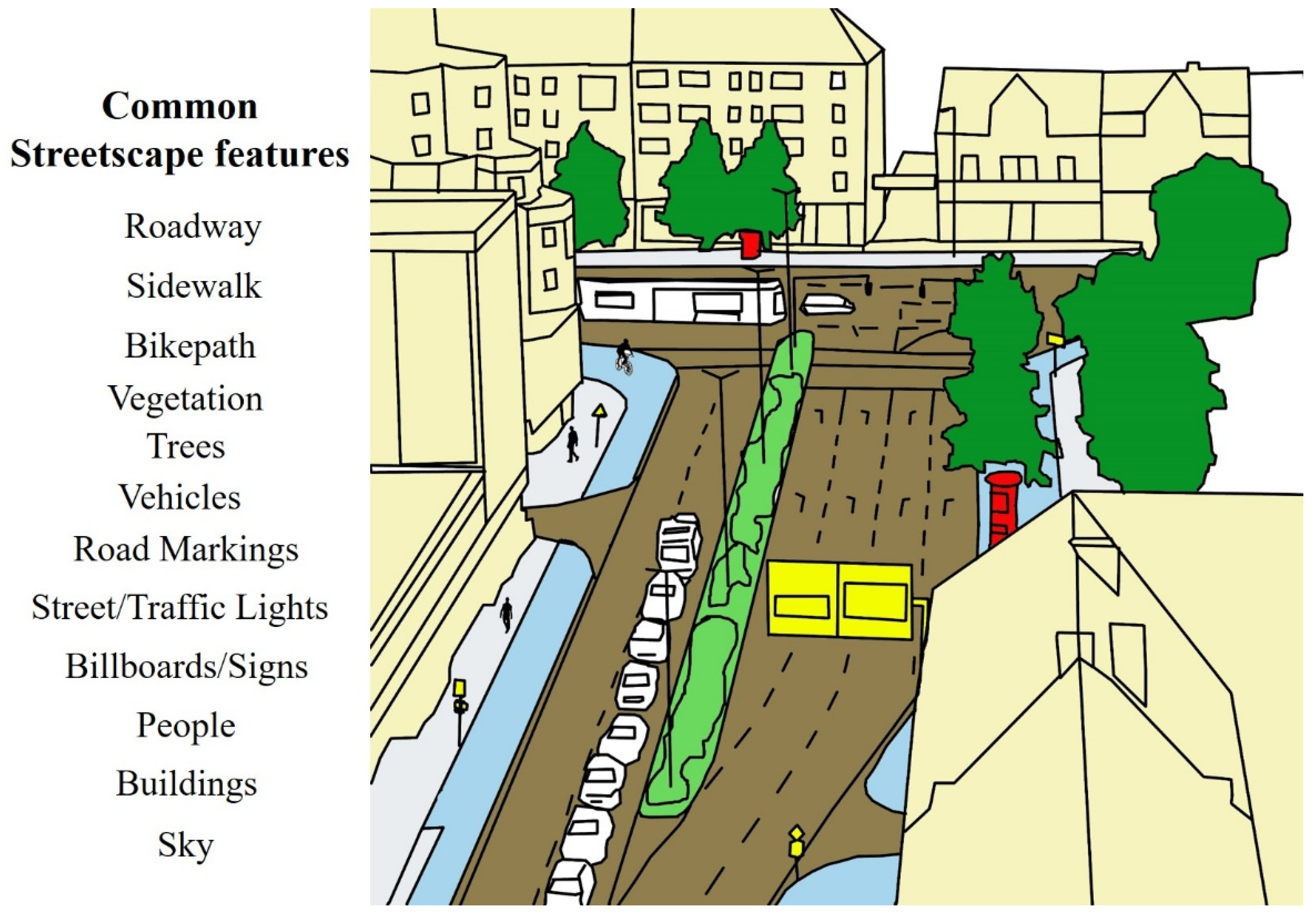
In recent years, research in autonomous vehicles has led to the development of a variety of algorithms that are efficient in classifying streetscape features (Figure 1), although from the street-level perspective. The datasets such as Cityscapes [26], Synthia [27], and KITTI [28], etc., collected with onboard sensors such as LiDAR scanner and multiple RGB cameras, have been since utilized in the training and evaluation of DL algorithms. Such datasets and models are widely available in the open research domain and have generalized well enough to detect and classify common streetscape elements from street view imagery.
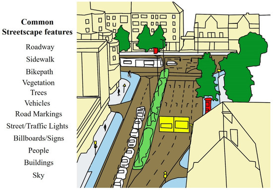
Figure 1.
Illustration showing common streetscape features in cities.
While subjective assessments and identification of streetscape features through the on-street perspective have been researched mainly through photographic evidence, the comprehensive DL-based 2D and 3D mapping of these features from overhead imagery have been comparatively less interesting. Earlier studies utilizing satellite or aerial imagery for urban mapping [29,30] dealt with the issues related to the resolution of the captured image or the unavailability of robust algorithms to automate or train the models. Therefore, detailing out urban features using traditional methods lacked precision and consistency. Since DL and Very High Resolution (VHR) resources have slowly become available to researchers, the conditions could not have been riper for further investigation. Furthermore, ever-expanding Earth Observation (EO) databases accompanied with DL methods allow detection and delineation of a broad range of urban features such as building footprints [31], vehicles [32], streets [33], and trees [34]. Also, DL models have better generalizability than traditional image processing methods; hence they can be scaled to cover multiple cities or regions.
Urban areas are composed of multiple components, of which buildings, trees, and streets are fundamental in defining streetscapes (Figure 1). Detecting building footprint from the imagery has been instrumental in studying urban neighborhoods, morphology, density, and demographics [35,36]. The detection models are an upgrade to existing building footprint databases such as OpenStreetMap (OSM), which were prone to errors and coverage due to the crowdsourcing. However, due to the lack of height information in VHR satellite imageries, the DL models are blind to the heights of the buildings, which is a vital component of the streetscape. Studies have utilized LiDAR-based mapping systems [37] to generate a precise measurement of the building heights. However, the availability of such datasets has always been a concern. Recently, administrative agencies have started providing detailed building maps based on Open Geospatial Consortium (OGC) standards [38], including height and other administrative information with various Levels of Details (LoD) such as LoD0 (footprints), LoD1 (model created by extruding LoD0) and LoD2 (LoD1 with simplified roof shape individual components such as walls), which has been beneficial to urban research.
Trees have been vastly attributed to their contribution to understanding environment psychology, visual aesthetics, and crime [20,39]. Within the past five decades, EO data-based Tree detection and identification has undergone a massive makeover. The satellite imageries had been used to estimate the amount of flora and biomass for ecosystem studies. However, given the coarser optical resolution of available datasets, these studies were practical only when studying regional green cover characteristics [40]. Recently, with the availability of sub-meter pixel resolution datasets, these studies can now be integrated into complex urban areas with better accuracy. Efforts have been made to identify trees from DL models and EO datasets; however, the focus of such research pieces has specifically not been in urban areas [41]. Detection of trees in urban areas is complex due to a variety of reasons. Unlike buildings, trees and vegetation are ephemeral, climates dependent, and prone to massive change over a short duration due to everyday upkeep, uprooting, aging, change in seasons, etc., challenging widely used DL methods.
Similarly, identifying streets from satellite and aerial images has gathered a lot of interest in recent years. The research has been primarily focused on identifying streets where the road network data is not available. Besides detailing street network maps for these settlements, multiple studies have extended the understanding of infrastructure development, settlement growth, and planning evacuation routes during natural and man-made hazards [42]. In addition, a large part of the research has evolved to understand pedestrian and bike accessibility, connectivity, the liveliness of the streets. Such studies have explored multiple ways to extract street information from the aerial and EO datasets.
The discussed studies provided a vast literature describing tools and techniques to use EO datasets to capture detailed urban features. However, such studies have been conducted independently and focused on few urban features at a time. This provided an opportunity for us to realize the potential of new research, which builds upon the earlier literature and integrates multiple datasets and independent DL models under one umbrella. Apart from the discussed streetscape elements, this study attempts to classify fine-grained features present in the urban streets such as (a) corridor (b) roadway, (c) sidewalk, (d) bike path, (e) on-street parking, (f) trees, (g) road markings, (h) vegetation, (i) vehicles, and (j) buildings. Various DL methods and open-source datasets are tested to develop robust classifiers that can detect these features with precision. The output of the entire process results in GIS-based vector datasets comprising identified elements in the imagery. The obtained geospatial dataset is used to study street cross-sections in this study. It can be further utilized as a database for studying the design and physical quality of streets and their impact on pedestrians and cyclists. As the process produces trained DL models, the study can be repeated in different cities to compare a variety of streetscape qualities.
2. Methodology
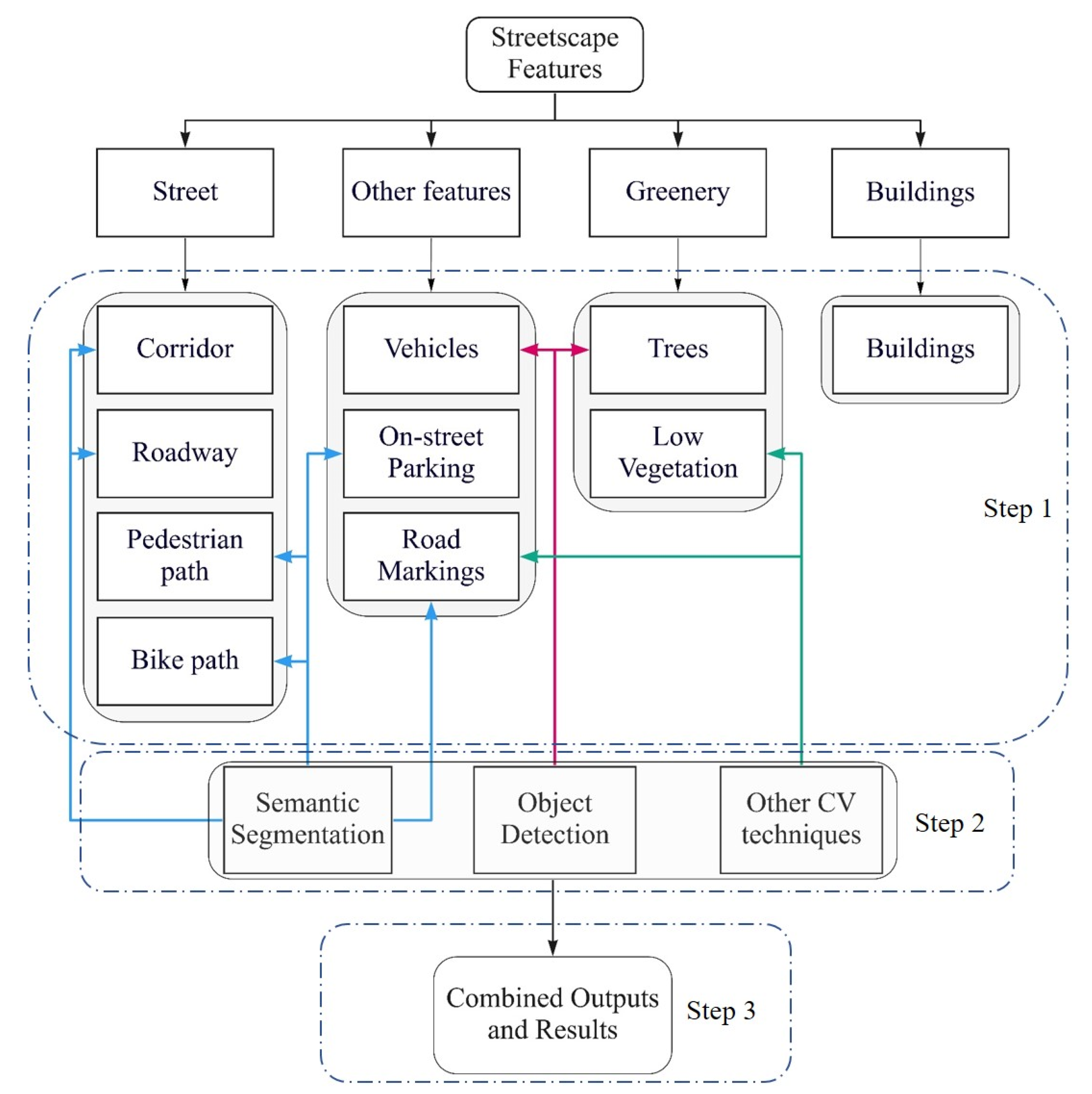
The study is broadly divided into three parts (Figure 2). Firstly, the selection of streetscape elements is finalized, given the availability of training datasets such as VHR satellite/aerial datasets and associated annotations. This step is especially relevant as elements such as street/traffic poles and lights and billboards (Figure 1) are pertinent in streetscape visualization and understanding; however, no openly accessible datasets are available to build and train the models to identify these elements. In the next step, experimentation is done to select the best model for identifying each feature identified in the first step. Next, commonly used metrics are utilized to judge the model performance in the study area. Finally, the outputs from the individual models are integrated to create a street-based geospatial dataset and its virtual representation in a 3-dimensional context.
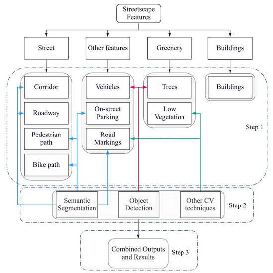
Figure 2.
Flowchart showing the overall methodology of the study.
2.1. DL Techniques Used in the Study
Object detection and semantic segmentation are computer vision (CV) tasks that involve identifying specific features in the imagery. These tasks are achieved by robust neural network architectures, which outperformed several traditional CV methods dealing with similar tasks such as SIFT, SURF [43], etc. These model architectures utilize Convolutional Neural Networks (CNN), designed to extract relevant features and learn representations inherent to the images through the backpropagation method and custom loss functions. The model is “trained” when it can no longer learn new information from the data and update its learned information or “weights”. These weights are repurposed as pretrained models and can be saved as a standalone file for further inference in new datasets. While the building blocks for both detection and segmentation tasks are similar, they fundamentally differ from the application point of view. For example, object detection models produce bounding boxes corresponding to each trained class in the image, while segmentation classifies each pixel to create a mask for each category. Therefore, the detection models are best for identifying locations of the elements in the image but do not give information on the shape of the particular element. On the other hand, segmentation models can provide such details; however, they do not separate such instances similar to detection tasks. Filling the gaps in both models, instance segmentation models achieve the best of both, detecting and delineating the distinct elements trained in the model.
Like other Machine Learning (ML) models, DL models are data-intensive algorithms. The availability of large sets of training data dictates the overall model performance. Object detection, semantic segmentation, and instance segmentation can be listed in order of increasing difficulty in data annotation and hence the difficulty in obtaining annotated datasets for these tasks. This study mainly utilizes semantic segmentation for mask generation of street features and object detection to identify vehicles and trees. All the models are trained with the help of one Nvidia Tesla P-100 GPU with 16 GB VRAM. A variety of data sources and models are used, the information regarding which is discussed further.
2.2. Data and Model Sources
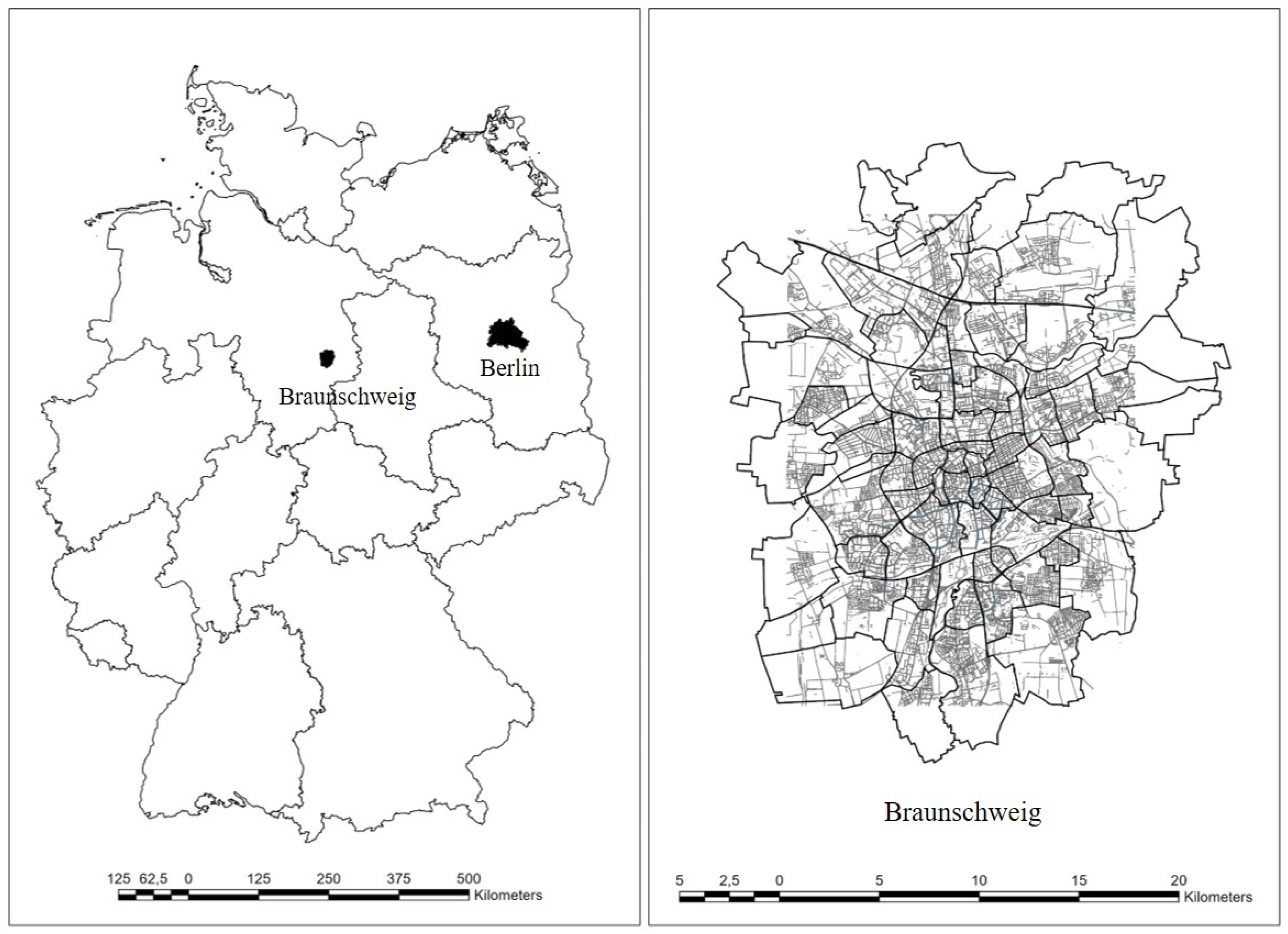
Braunschweig, a city in Lower Saxony federal state in Germany, is chosen as the study area (Figure 3). The city has a population of 0.25 million and has an administrative area of 192 sq. km. We used a VHR aerial image dataset covering the entire city. The imagery was acquired using low altitude aircraft and is part of a larger data collection project performed over various German cities [44]. The image data was available as tiles for which the Orthomosaic was created using ArcGIS. The final imagery was further subsampled to 0.2 m/pixel to suit the requirements of the models used in the study (Table 1).
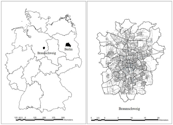
Figure 3.
Map showing the location of the city of Braunschweig.

Table 1.
Selected streetscape features and data sources used to acquire imagery and models.
Apart from the VHR data for the study area, this study further utilizes multiple sources to collect training data and pretrained models (Table 1). One of such vital sources is Geoportal Berlin FIS-broker [45], which provides geospatial datasets for the city of Berlin, including VHR satellite imagery. The dataset was created in 2014 and updated in 2019, paired with accompanied VHR satellite imagery at 0.2 m/pixel resolution captured in February 2021. This study utilizes a “Straßenbefahrung 2014” dataset from FIS-broker, consisting of detailed mapping of street-level characteristics. The data is available in WMS (Web Map Services) and WFS (Web Feature Services), which can be downloaded in raster or vector format, respectively. Some of the features included in the dataset are fountains, parking ticket machines, guardrails, hydrants, curbs, display boards, among other standard features such as roadways, bike paths, sidewalks, etc. While most minor features are not discernible through the imagery provided, the inference on major street-level features can be easily made. Five major street-based classes such as corridor, roadway, bike lanes, sidewalk, and on-street parking are utilized from the dataset and separately trained using semantic segmentation models.
This study also utilizes the pretrained object detection model, DeepForest [41]. The model has been trained on tree annotations in high-resolution image data. Although the trained model is primarily effective in forest and non-urban areas, further processing is done to suit the objectives of this study. Along with the obtained bounding boxes from the object detection model, pixel-wise classification was implemented to map low vegetation. It helped in mapping green medians along with tree cover in the streetscapes.
Object Detection is used to identify vehicles, more specifically, cars, with the help of the Cars Overhead with Context (COWC) dataset [46]. The dataset comprises 33 k annotated labels from Canada, Germany, the U.S., and New Zealand, along with 15 cm/pixel resolution image tiles.
Street markings dataset was generated with the help of standard CV techniques and the semantic segmentation approach. The image and masks were created from the imagery of Braunschweig City. Finally, the vector data for buildings was taken from the administrative website [47] as LoD 1 dataset. The particular approach is preferred over opensource databases such as OSM to accurately represent building heights.
2.3. Evaluation Metrics
Evaluation metrics are used to measure the quality of the trained model. The metrics are critical to model building, where they provide constructive feedback to modify the model throughout the process. Two commonly used metrics are Intersection over Union (IoU) and Mean Average Precision (mAP). IoU, also known as the Jaccard index, is the Area of Overlap between the predicted and ground truth boundaries divided by the area of union between both. The metric ranges from 0 to 1, where 0 corresponds to no overlap, and 1 signifies perfect overlap. IoU is a broadly used metric in Semantic Segmentation tasks. Other variations of IoU metrics, such as Weighted IoU and Mean IoU, are also commonly reported in the research. These are especially relevant in multi-class segmentation models. This study develops individual training models for each class, hence reports only the IoU metrics. The mAP is a popular metric in measuring the accuracy of object detection tasks. The metric calculates the precision given as the ratio of true positives and all the predicted positives. It also calculates the Recall metric of the detector, which is given as the ratio of true positive and total ground truth positives. The detection is considered positive if the value of IoU is more than 0.5. Precision-Recall curve is plotted from the obtained results. The area under the curve is termed Average Precision (A.P.). The mAP is the average of A.P. calculated for each class. In this study, one class is trained in both models (trees and vehicles); hence A.P. and mAP can be used interchangeably.
Since this study utilizes a collection of DL methods to obtain classification results, individual accuracy metrics do not do justice to the outcome of the final output. To understand the robustness of trained models, we manually annotated a small area in our study area (Braunschweig) and evaluated the metrics on the annotated data. For this purpose, the study area was divided into a grid of 500 × 500 m. A total of 150 tiles were prepared through this method. Further, 15 tiles (10 percent) were randomly selected from the total. These grids are further divided amongst the authors to prepare annotations for each class. ArcGIS Pro was used to create polygons and bounding boxes. The particular focus was given to ensure maximum detail possible in making the annotations, especially creating vegetation and road markings polygons. The whole process took 40 human hours. Throughout the study, IoU performed over testing data from the collected data is termed IoUd, while IoUs indicate evaluation performed in the study area. Similarly, mAPd denotes evaluation on testing data, while mAPs denote evaluation performed in the study area.
3. Model Creation and Analysis
3.1. Semantic Segmentation of Street Features
Most of the street delineation and mapping literature focuses on identifying the linkages of street networks as a single line representation rather than identifying road pixels. One of the reasons is the unavailability of large-scale training samples to train models for the latter scenario. The datasets regarding identifying linkages or the single line representation had been widely available. Researchers [48] have used crowdsourced datasets such as OSM streets as labels to train various models. Alternatively, representing streets as a single line is relatively straightforward than pixel-wise labeling if annotated manually. The other reason being the scale of the study area and purpose. Information on street linkages is relatively more important in routing and connectivity than determining pixel-wise street details. However, both approaches are not immune to the challenges related to the occlusion due to shadows, trees, buildings, scale, and resolution of the dataset. Researchers have devised various methods such as RoadTracer [49] and DeepRoadMapper [50], focusing on linking the misclassified street segments. However, these methods have not been applied to pixel-wise street segmentation models.
Streets have complex characteristics, unlike distinct classes such as buildings, trees, and vehicles, the definition of streets differs accordingly with the project requirement and the usage of terminology. Identifying pixels in which the vehicle moves (roadway) might be sufficient for the research which focuses on analyzing multiple large cities. However, studies that intend to focus on detailed characteristics of the streetscapes require exhaustive analysis. This study focuses on achieving pixel-wise classification of five significant subdivisions of “streets” such as (a) roadway, (b) sidewalk, (c) bike path, (d) movement corridor, and (e) on-street parking.
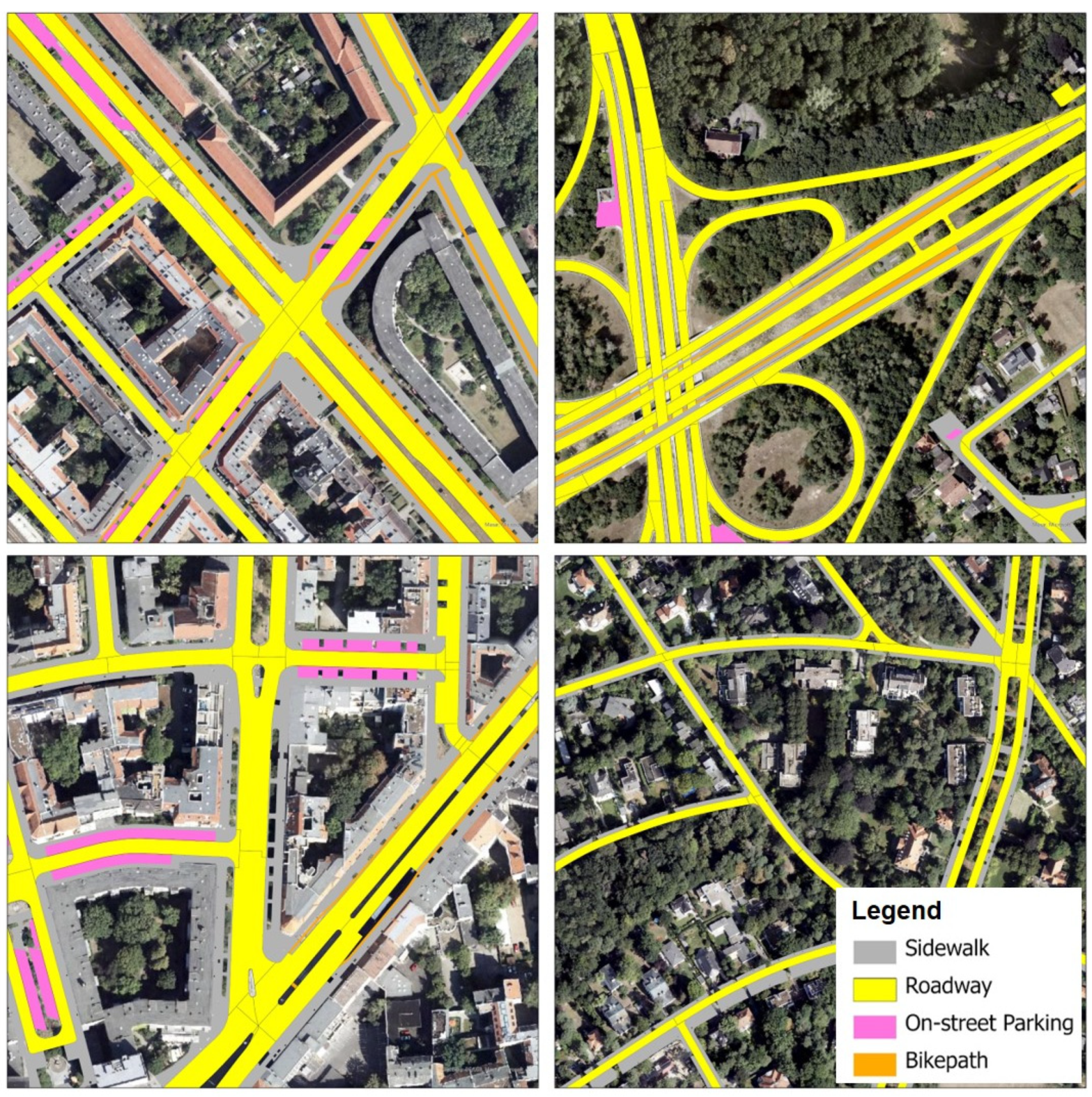
For this study, the roadway is defined as a path utilized only by vehicles (Figure 4). These are the dedicated lanes for use only by vehicles, while sidewalk and bike paths are used only by person on foot or bike, respectively. On-street parking, parallel or adjacent to the roadway, is common in many streets in Germany; hence it is an essential component of the streetscape. The on-street green spaces are widely present in the medians and show significance in the streetscape along the sidewalk. The discussion on delineating green spaces is discussed in the following subsections. The movement corridor is defined as a whole space encompassing all the above characteristics, usually covering the entire space between buildings located opposite the street. In other words, the corridor covers all the areas available for movement through any mode. However, the corridor concept does not apply in this study if the streets do not have a designated roadway. The FIS-broker does not have a “Corridor” as a separate class; hence the other street features are merged together to create one.

Figure 4.
Common street features available in FIS-broker [45] dataset.
The FIS-broker dataset (Figure 4) is converted as binary labels and VHR Berlin satellite imagery to train segmentation models. Three widely discussed segmentation models, such as U-Net [51], DeeplabV3+ [52], and D-Linknet34 [53], are used in the study. Initially proposed for biomedical tasks, the U-Net has shown exceptional performance in various domains, such as regular images and street view images for research on self-driving cars. U-Net has also been widely used in satellite segmentation tasks [54,55]. Vanilla U-Net using Resnet-50 [56] backbone is used in the study. DeepLabV3+ [52] extends the DeepLab model, introducing the atrous or dilated convolutions to extract denser features and capture multi-scale context by varying atrous rates. DeeplabV3+ showed state-of-the-art performance on PASCAL VOC [57] and Cityscapes [26] dataset. D-Linknet34 is a LinkNet [58] Architecture modification, which demonstrated its applicability in efficient segmentation tasks. Similarly, D-Linknet34 uses ResNet34 pretrained on ImageNet as its encoder and LinkNet as its decoder. The model is designed to include larger receptive fields and dilated convolution layers with skip connections to enhance the segmentation outputs. It utilizes BCE (binary cross-entropy) with dice coefficient loss as loss function and Adam as the optimizer. The model won the DeepGlobe [59] road extraction challenge in CVPR 2018. The challenge included 2000 high-resolution images (0.5 m/pixel) and masks from Thailand, Indonesia, and India.
As opposed to treating the task as multi-class segmentation, each of the five street-based features was independently trained. This was required for three critical reasons. (a) As discussed earlier, the corridor class overlaps with the sidewalk, roadway, street parking, and bike path classes; hence it cannot be simultaneously used as a multi-class segmentation task. (b) Roadway, sidewalk, street parking, and bike path classes do not have the same pixel distribution; therefore, better performance is difficult to achieve by collectively training these classes [53]. (c) Independent training further assisted in validating the results obtained from all the individual models.
While experimenting with various segmentation models, it was observed that the scale and resolution of training tiles affect the model’s performance; hence, different tile sizes were tested along with chosen segmentation models before selecting 1024 px × 1024 px size. It is further realized that in a given a consistent NxN pixel size to be used in the model, while the higher resolution of the data can provide detailed information of a location to the model, it can simultaneously deprive it of assessing its neighborhood.
A total of ~12,000 tiles each of satellite image and binary labels with the size of 1024 × 1024 px obtained from FIS-Broker are used to prepare a dataset to train each of the five individual streets elements. 20 percent of the data is randomly chosen from the dataset for each model for testing. Augmentations such as randomized values of Hue-Saturation-Value (HSV), Shift-Scale-Rotate, Horizontal and Vertical flip, and Rotate are used to help the model generalize better to the training dataset. The individual models are trained till the losses cannot improve further. The time taken by each of the three segmentation models to train varies. The DeepLab V3+ model is the fastest with 16–24 h across each of the five street-based features, followed by U-Net with 20–30 h, and D-LinkNet34 with 24–36 h.
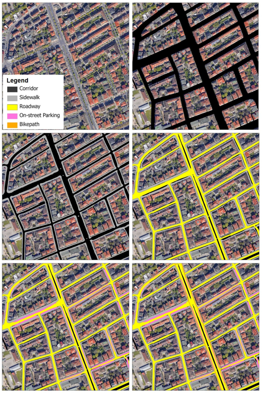
Figure 5 shows the performance of various classifiers in the segmentation task. The D-LinkNet34 model offers comparatively better performance in the test set as well as the study area set. Further, the difference between IoUd and IoUs is less than the other two models, suggesting better generalization capability of the D-LinkNet34 model. However, the performance of all the models in detecting on-street parking and bike paths is relatively similar. This can be attributed to the reason that comparatively fewer instances of these classes are available in the dataset. In addition, the width of the bicycle path and parking locations are significantly narrower than the roadway or sidewalk, which gets even more prominent when considering the resolution of the satellite imagery (0.2m/px). Further, the shadows from roadside trees and buildings adversely affect the identification of these classes.
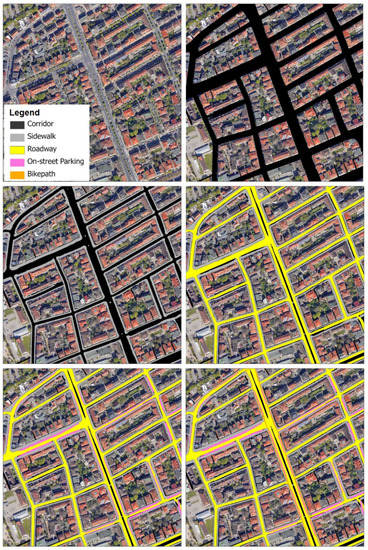
Figure 5.
Tiles showing output from the D-LinkNet34 segmentation model in the study area.
Table 2 shows the output of the trained D-LinkNet34 model on all 5 features. The model demonstrates its effectiveness in learning various road features with varying degrees of narrowness. In addition, the model performs well on frequent occlusion without compromising on connectivity. However, it is seen that the model is affected by the color of street material, especially in the case of Roadway classification. Training data [45] roadway labels mainly comprise bituminous-based paths; hence, the model finds it challenging to identify the street with pavers, cobblestones, or concrete. Although the issue’s magnitude is still minimal, the study area, being a German city, has similarities with Berlin in terms of the street layout. However, the problem may get pronounced when using a study area at a different location. Further, the model finds it challenging to detect the parking locations where the vehicles are parked parallel to the street. This behavior is more prominent in the narrower streets. The model’s inability to judge the vehicle as a parked one vs. moving in the roadway is the main reason.

Table 2.
Evaluation metrics (IoU) of five street-based features. Values in bold indicate best performing models.
Since the imagery is used in the models as tiles, the outputs are needed to stitch together to create overall maps. The production of the stitching process includes multiple artifacts; hence the issue needs to be addressed appropriately. Iglovikov et al. [60] used the strategy to crop the output masks from all sides before stitching, while Huang et al. [61] used an increased input patch size during inference. This study utilizes a model averaging with a spatial displacement approach [62], where the overlapping tiles are fed to the model and masks are overlapped to create a resulting map (Figure 5).
3.2. Trees Detection and Vegetation Classification
Tree and vegetation identification in urban areas has been quite relevant from the perspective of health and wellbeing, ecosystem services, urban forests and wildlife, and microclimatic provisions. The information regarding the location and size of trees is vital while designing and framing urban planning and design provisions and studying their impact on walkability. Studies have utilized aerial and terrestrial datasets such as street view imagery [63] to generate detailed treemaps. Understanding the role of trees in daily urban life, such as shade provision, urban heat island reduction, ornamental and greenery, pollution compensation, wellbeing, and urban aesthetics is ongoing research. Accurate identification of tree locations and sizes may help expand the context and scale of such studies.
In this study, the estimation of tree locations is essential from the perspective of creating streetscapes. Object detection model and unsupervised pixel-wise classification method are utilized to identify trees and green spaces, respectively. While instance segmentation might have been a proper method to identify individual trees and classify them, the procedure is not implemented due to the unavailability of instance segmentation datasets. Instead, the detection model provides bounding boxes with which the tree trunk can be estimated, which is necessary to represent trees in street cross-sections and 3D models.
The tree detection utilizes a pretrained DeepForest model. The model is trained on the widely used object detector RetinaNet [64]. The model employs Feature Pyramid Network, which specializes in detecting objects at different scales, and uses the Focal loss function, which removes the class imbalance between foreground and background. The model is sensitive to the size of the image tile provided for the predictions. As the model was trained with 0.1 m/px resolution imagery and 400 px × 400 px dimensions of the tile, the evaluation for our use case is done at 800 px × 800 px, since the study area has a resolution of 0.2 m/px. The pretrained model shows rather average performance in the study area with mAPs of 0.774. The main reason for the performance is the dataset on which the DeepForest model is trained. DeepForest utilizes labeled instances of trees located in forests and non-urban areas. Therefore, the dataset does not include the samples of trees in urban or built environments. As a result, the model misclassifies specific geometries in an urban environment, such as gabled roofs and hedges for trees. Further, the model has been trained on higher resolution image data, which affects tree detection.
To solve this issue, it was decided to finetune the trained model to include few samples from the urban environment, which would help the model generalize well enough to detect trees in urban areas. Therefore, the dataset was created from the study area VHR imagery image tiles at 800 px × 800 px.
An open-source software LabelMe was used to create a total of 2000 samples from 115 image tiles. The model training is performed using the pretrained model with the new dataset. The model was trained for 27 epochs before loss did not improve any further. The training took approximately 10 min. With the new model, the mAPs showed significant progress from 0.774 to 0.878. Similar to the segmentation model, the object detection model utilized here is also prone to edge effects. Inspired by the original DeepForest RetinaNet model, we use an overlapping factor of 0.1 to produce outputs.
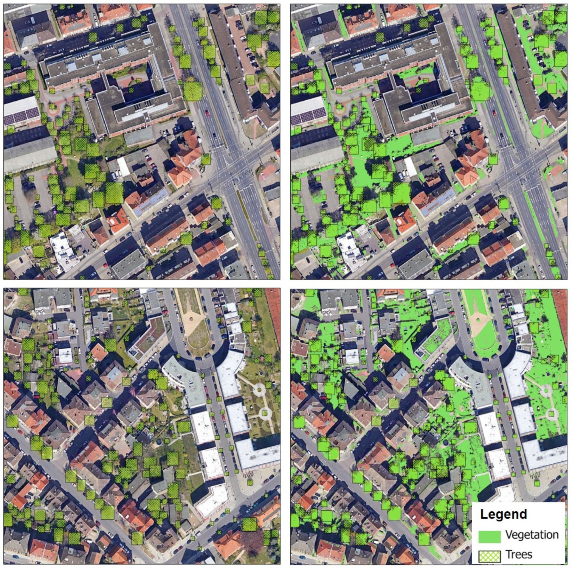
Surprisingly, the model performs well given the tree crowns’ complex spatial and spectral signature (Figure 6). The model identifies trees even with smaller crowns, which are prominent in the streets. Although identifying trees other than on streets is not essential for fulfilling this study’s objective, the models’ performance in detecting tree cover in parks and open areas is a huge plus. Given the transient nature of tree crowns which depend upon the seasons, the discussed model can be finetuned with the data collected from the winter months to further create a robust urban tree detector.
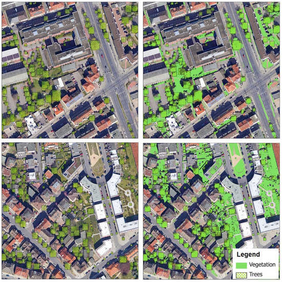
Figure 6.
Tree detection and Vegetation classification output in the study area.
Apart from the Tree detection, Iso clustering unsupervised classification is conducted on the imagery of the study area for classifying vegetation. The main objective of this task was to isolate green pixels, which is done by selecting a few of the obtained classes from unsupervised classification and reclassifying them as vegetation. The process results are promising (IoUs of 0.812) and can delineate roadside greenery with great precision (Figure 6). The only downside of utilizing this approach is that it only picks up the green spectral signature, which might not represent the entire area with vegetation. Furthermore, depending upon the image acquisition time, the foliage may exhibit various textures, patterns, and colors, which might be difficult to capture via this method. The alternative strategy would be to utilize semantic segmentation and annotated labels. However, the results from the unsupervised classification fulfilled the purpose of this study; hence segmentation approach was not used.
3.3. Vehicle Detection
Methods to detect vehicles from overhead imagery have been researched, mainly for knowledge discovery, understanding mobile assets, search and rescue, and parking locations. Compared to other DL tasks listed in the study, detection of vehicles, primarily cars, are more straightforward due to the distinct visual features in contrast with the overall environment. For example, vehicles can be located in the urban environment with a distinctly visible background of the street or a paved area. It is inherently different from tree detection, where the probability of locating a tree in green vegetation as a background is higher.
The RetinaNet object detection architecture is trained using the COWC dataset. The data is divided into 80:20 for training and testing. The model was trained for 155 epochs with a batch size of 32 till loss could not decrease further. It took around 4 h to train the model. The obtained mAPd of 0.930 was considerably higher than mAPs of 0.816. Common reasons for such a difference in metrics may include (a) the difference in resolution in the dataset and the study area. The model training is done on the images with a slightly higher resolution of 0.15 m/px than the data resolution in the study area (0.20 m/px). (b) Further, it is observed that the training dataset includes fewer samples in which vehicles are located where occlusion from the tree canopy and building shadows is present.
As a result, similar to the manually drawn labeling in tree detection, a total of 1000 instances from 340 image tiles with the size of 256 px × 256 px were manually annotated from the study area with the help of the LabelMe application. These instances are then fed to the trained vehicle RetinaNet model for finetuning. After training for 54 epochs, the model provided mAPd and mAPs of 0.930 and 0.912, respectively. The training time took approximately 20 min. An overlapping factor of 0.1 is used to produce outputs. It is reassuring to see that the detector can achieve relatively high accuracy even with fewer training samples used for finetuning.
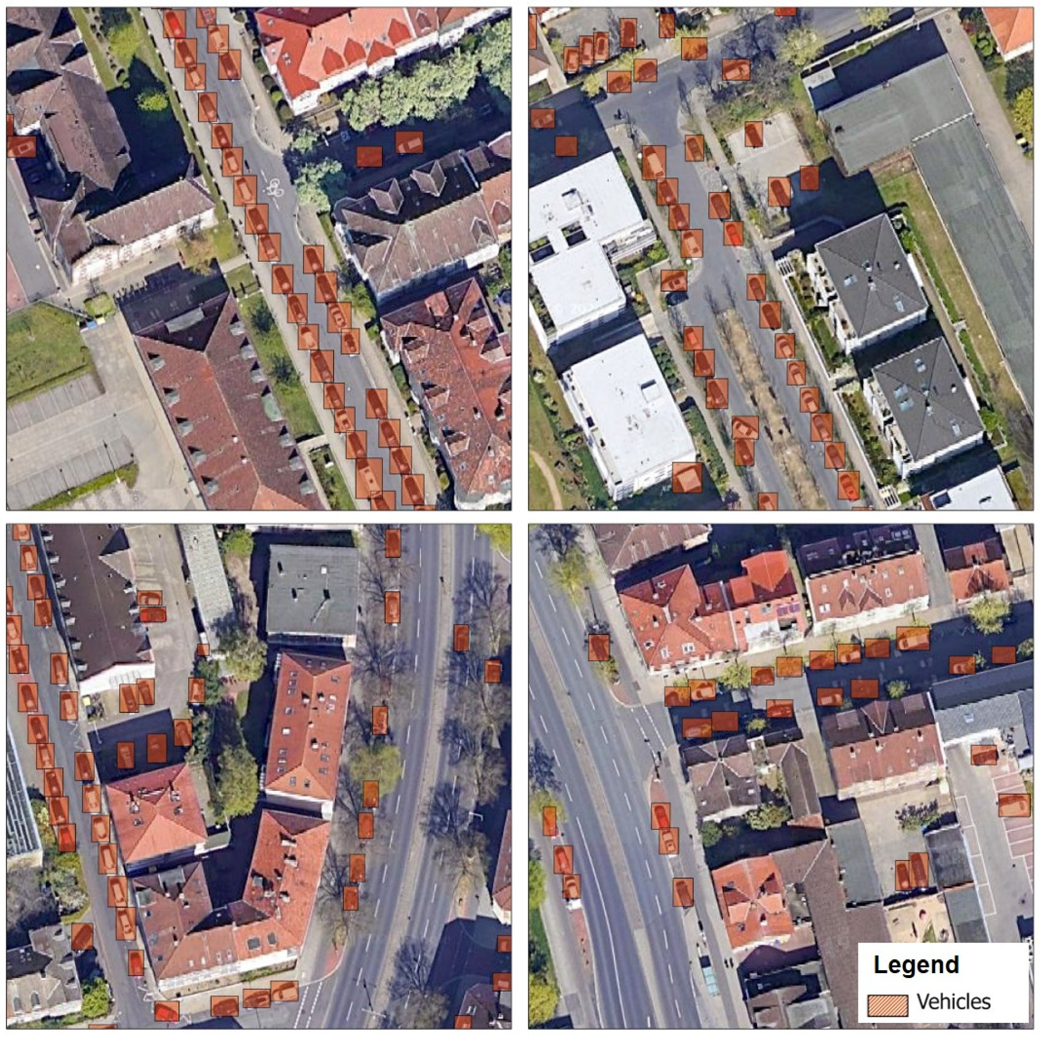
As evident in Figure 7, The detector demonstrates superior performance in detecting vehicles, even the instances where only a part of the vehicle is visible or overshadowed. While the results look promising and robust, the detector is not trained to identify various vehicles. The training dataset comprises only cars; hence, the information regarding vehicles such as large trucks, buses, trams, etc., cannot be identified through this method.

Figure 7.
Vehicle detection output from RetinaNet object detection model in the study area.
3.4. Road Markings Generation
Road marking detection and classification has been widely researched from street view datasets [65,66]. However, road marking from aerial and satellite imagery is a comparatively recent quest to prepare high-definition routing maps for localization tasks in designing algorithms for driverless vehicles. The road markings are intuitively more distinct, given the consistency in shape, size, and color. Typical CV methods such as edge detection and morphological functions are well designed to isolate such shape instances from the images. However, various urban elements, especially rooftop edges, vehicles, and street poles, can be misrepresented as road markings using standard CV methods. Hence, its classification still requires support from context-aware DL Algorithms.
Researchers have created a markings segmentation algorithm named Aerial LaneNet [67]. Aerial LaneNet is a modified version of FCN Network, which integrates Discrete Wavelet Transform, which provides the network with different image representations at various scales. This property is similar to the D-LinkNet34 model used in this study for semantic segmentation tasks. Aerial LaneNet model is trained on AerialLanes18 dataset, which is RGB based 13 cm/px dataset. Similarly, related research [68] identifies such street markings with other detailed features. Both of these studies take the help of a large data set and masks created by annotators.
Apart from the other models, which utilized Berlin image data for training the models, this model uses study area image data. This approach was taken after realizing that Berlin data, although it has the exact resolution (0.2 m/px) as study area imagery, is not sharp enough to identify more minor features such as road markings. Therefore, the study area imagery is divided into 6 equal parts, of which one part is considered for the entire process of label creation and model training. The resulting area of the single part is 29 sq. km.
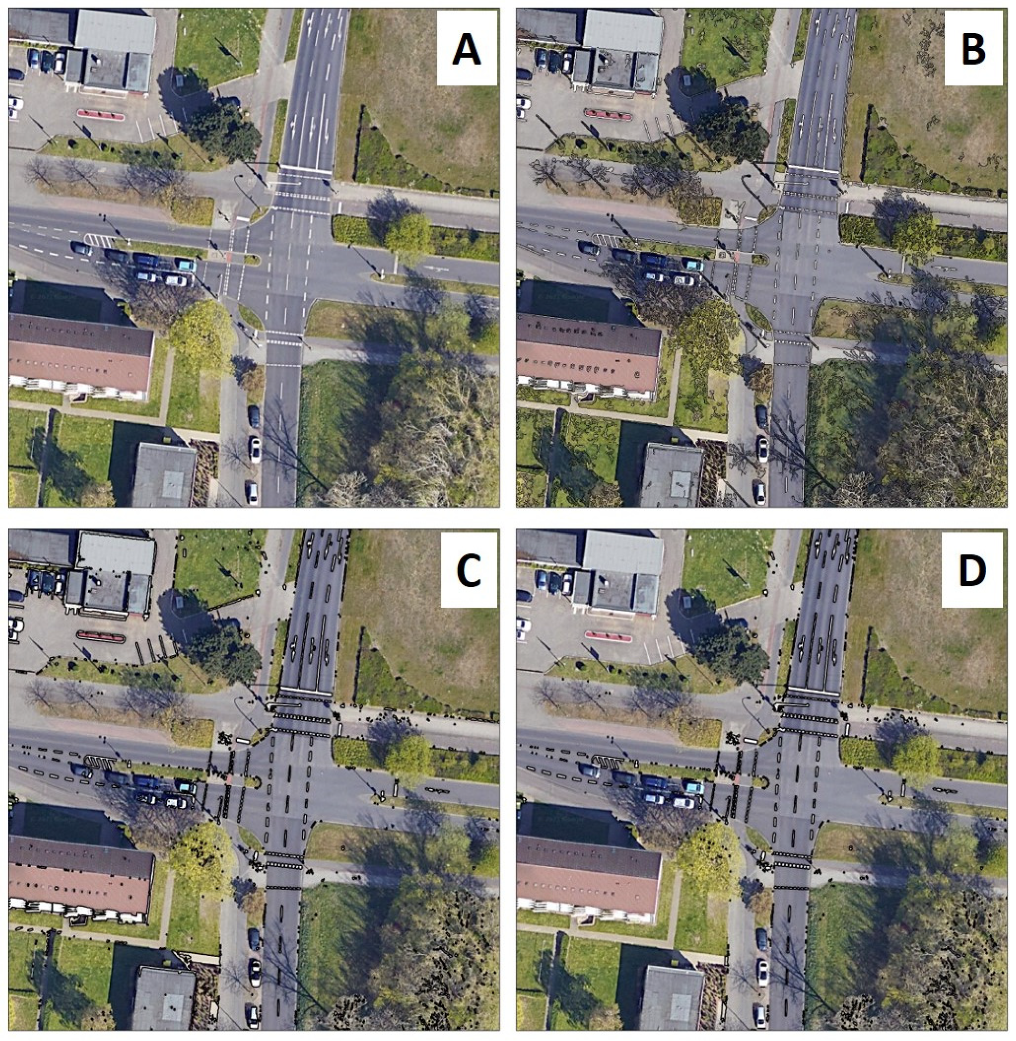
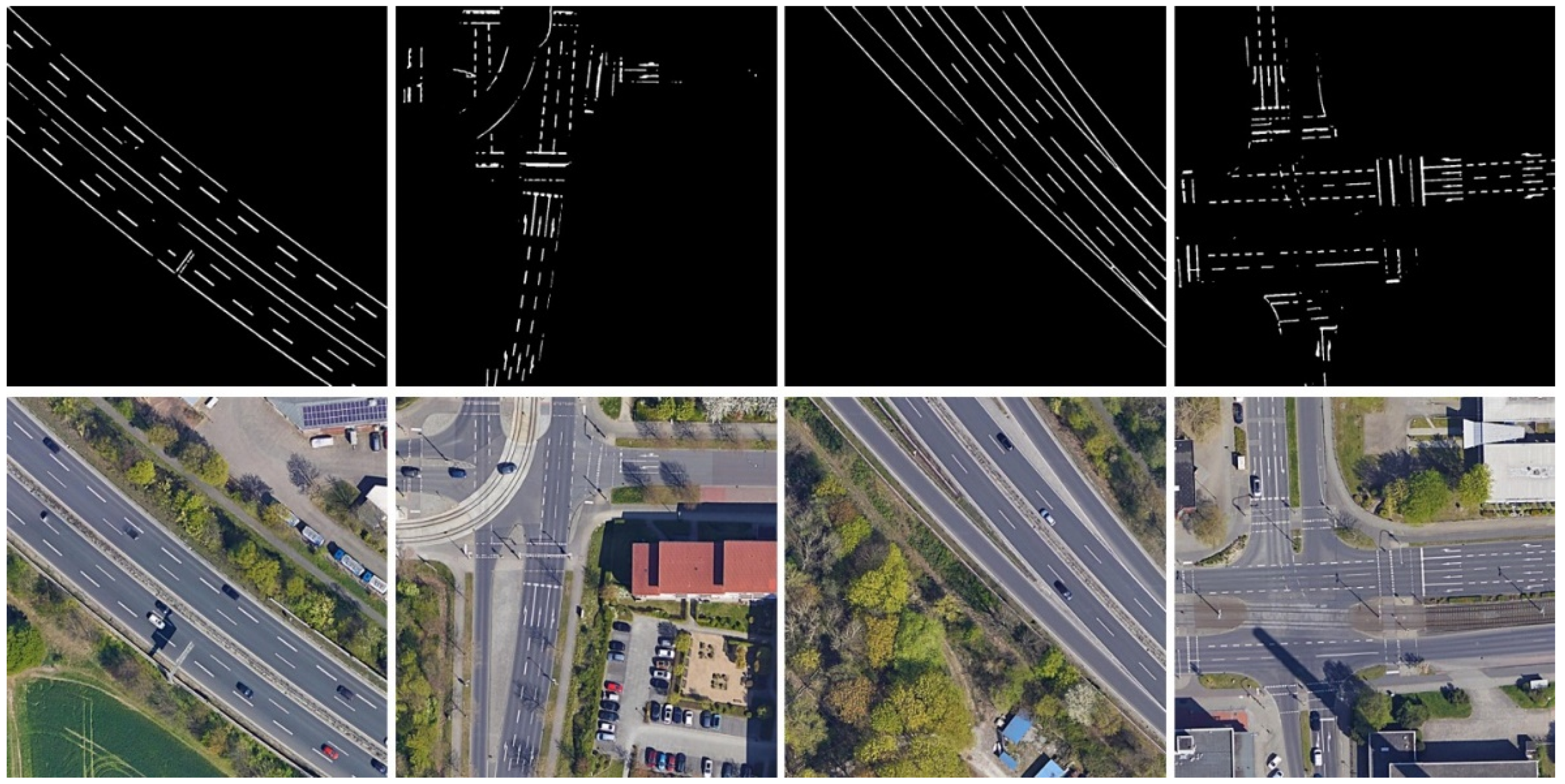
After the selection of the area, a two-stage method is applied to create a road markings model. The road markings masks are created by utilizing CV methods in the first stage, which are further used as training data to train the segmentation model. Firstly, in stage one, one of the popular CV algorithms, Canny edge detection, is performed, and the resulting output is used as an input to “expand” morphological function (Figure 8B). The edges detected by the edge detection algorithm leave few pixels, which are subsequently filled by the morphological method. The resulting output is converted to polygons, which automatically erases inadvertent single open edges. Secondly, the process includes the selection of white colors in the entire imagery. Iso-clustering unsupervised classification is used to select white colors in the imagery. This process isolates every white color in the imagery. Finally, the output from these two steps is overlapped. The overlapping pixels were retained while the rest others are erased (Figure 8C). The pixels identified with this method are further filtered to include only the pixels which are in the corridors (Figure 8D). The obtained markings, along with the imagery, are then used to create a road marking dataset. In the second stage, the D-LinkNet34 segmentation model is used to train the model with the help of the dataset thus created.
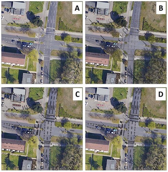
Figure 8.
Stepwise process (A–D) of creating road marking samples with computer vision algorithms.
Since the resulting image dataset is not large, an overlapping factor of 0.5 is considered to create image tiles of size 1024 px × 1024 px. A total of 3350 tiles were generated from the resulting imagery, further divided into 80:20 for training and testing the model. D-LinkNet34 model was trained for 47 epochs. The total training time was approximately 7 h. The augmentation and tile stitching strategies are kept similar to the street features segmentation (Section 3.1). The IoUd and IoUs were 0.721 and 0.693, respectively, indicating satisfactory road marking detection performance.
The model is efficient in detecting road markings (Figure 9); however, similar to other models, prone to misclassification due to shadows. The model performs well in leaving out the edges of buildings and vehicles in the street, which have a similar spectral signature.
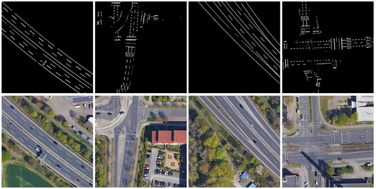
Figure 9.
Road marking output from segmentation model in the study area.
4. Combining Outputs
Collectively, a total of nine models are utilized to obtain common street features from VHR imagery (Table 3). Semantic Segmentation with the help of the D-LinkNet34 model is implemented for street-based features and road markings classification. The vehicles and trees are identified with the use of the RetinaNet object detection model. Classification of green vegetation is done with the help of an unsupervised iso clustering method. Since labels for road markings were not available, common computer vision algorithms such as Canny edge detection and other morphological functions were utilized to create such samples. The model weights of all the discussed models are available at https://github.com/deepankverma/streetscape_features, accessed on 28 June 2021.

Table 3.
Summary of training details of the streetscape features.
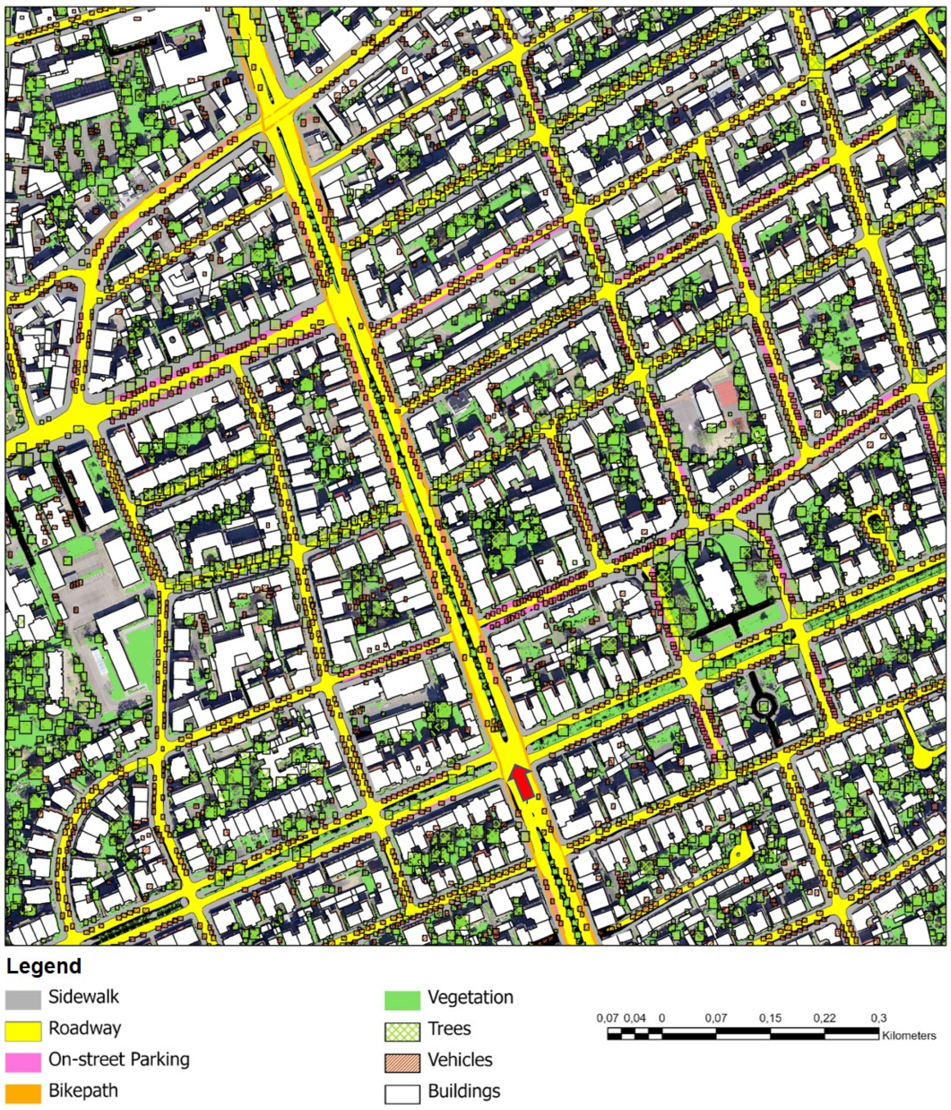
The outputs from the created models are converted to shapefile and integrated into a spatial database (Figure 10). The corridor is overlapped by other street features, hence not visible in the figure. In addition, buildings from LoD 1 are included. According to the building dataset [47], the city of Braunschweig has 98,865 buildings. The city’s average building height is 5.7 m, including garages and buildings in allotment gardens that mostly have one-story height. However, the buildings in the inner city (Figure 10) are 12–20 m in height. A total of 434 buildings in the city are higher than 20 m.
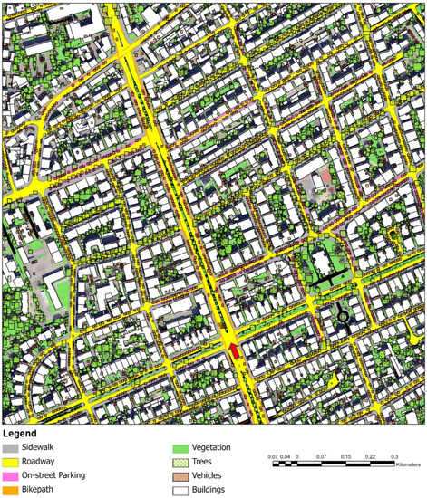
Figure 10.
Combined outputs from all the segmentation and detection models.
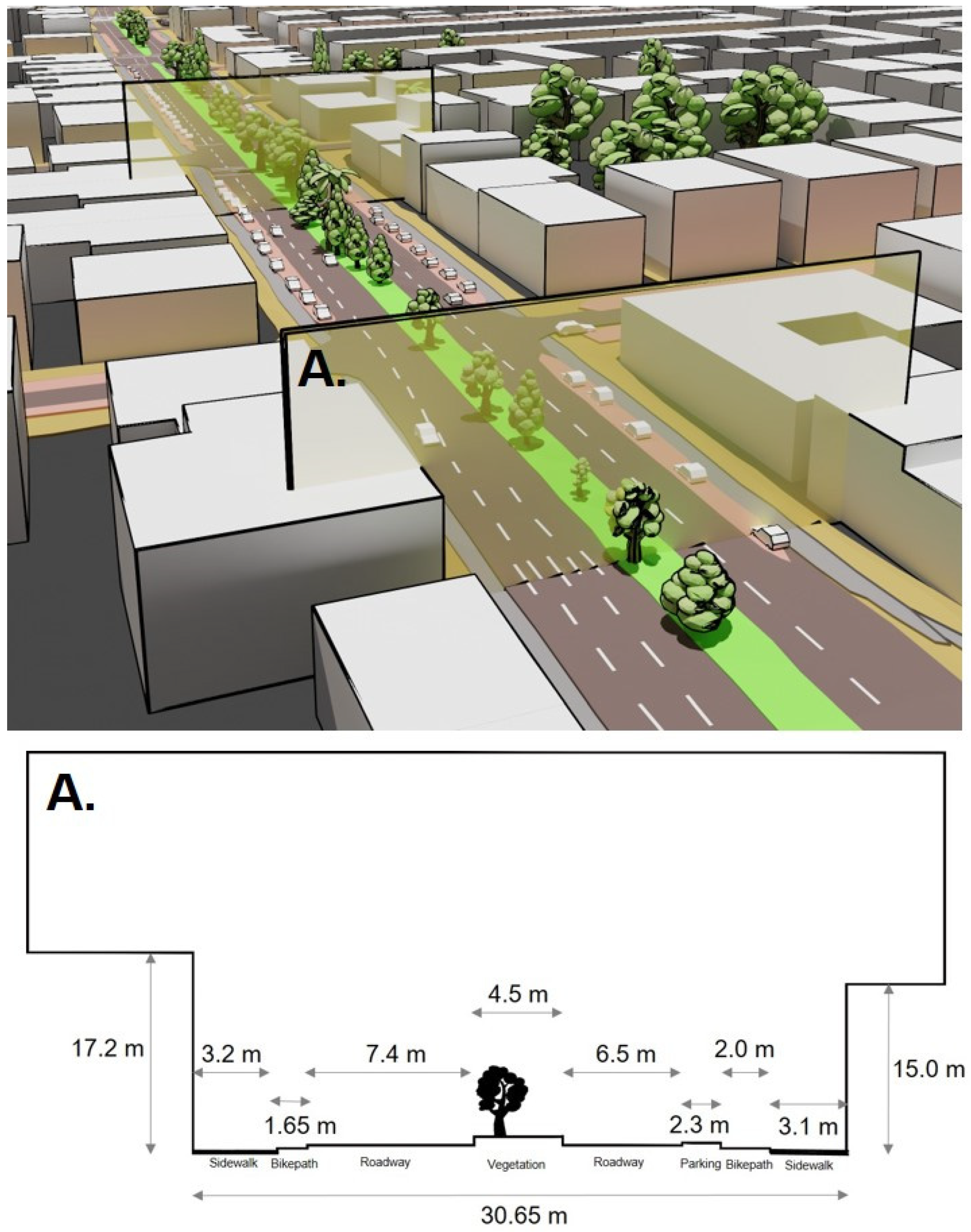
The generated combined geospatial dataset is further utilized to create street-cross sections with the help of Blender software (v 2.93). Blender is one of the industry-leading 3D computer graphics and media creation software and can integrate various workflows with maximum control over the user-defined processes. However, Blender maps its objects in Cartesian coordinates, which has limited applicability to our intent. Therefore, we utilized Blender-GIS plugin to import shapefiles in the software. In addition, Blender provided tools for rapid visualization of perspective views of the entire study area. It also offers powerful python-based scripting to rapidly automate repetitive tasks. Figure 11 shows the 3D view (from the location of the red arrow in Figure 10) and an example of a cross-section generated with the help of Blender modifiers and tools.
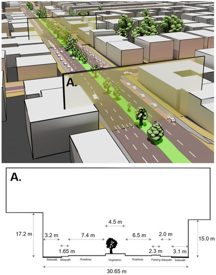
Figure 11.
Combined output translated to 3D model with specific cross-section.
These cross-sections are an effective abstract way to understand the city through its streetscapes. It communicates the overall movement set up in the particular location. In addition, they provide a practical understanding of the space designation for each mode of mobility and reserved space for vegetation or trees. Apart from giving an abstract visual representation of the streetscape, the measurements of the street features can be used directly to compare multiple locations and cities for potential improvements in walkability, vegetation, or vehicle movement.
The Blender-generated 3-D views show much resemblance to a virtual self-driving game-based engine such as the Carla simulator [69] and datasets such as Synthia [27]. Given the detailed generation of streetscape features, the 2D shapefile-based information can be effectively translated to 3D maps and used for different research problems such as autonomous driving or urban design and planning.
5. Future Directions and Limitations
The study proposes multiple strategies to create a geospatial database of streetscapes features derived from open data sources and DL models. Apart from the promising performance of the segmentation model, the object detection model with finetuning strategy yielded a higher accuracy for the detection of trees and vehicles. The study is unique as it combines multiple individual features, which results in a geospatial dataset and can be easily used as part of urban research focused on understanding the city’s general makeup across various scales. While OSM datasets have been used by researchers for estimating morphology and road network connectivity, this method further adds pixel-wise classification to distinguish between different features present in the streets. In addition to street cross-section, other urban design methods such as Isovist properties [70], perimeter, maximal radials, occlusivity [71], compactness, and axial connectivity [72] can be achieved by 3D streetscape generation. Moreover, such 3D models can be used in AR/VR platforms to conduct individual preference-based studies.
Although the study is a successful attempt to classify major streetscape features, few limitations must be discussed. First, the generalizability of the proposed models, especially the segmentation models, is not guaranteed in other cities. Since DL models learn representations from the datasets on which they are trained, the results on unseen datasets may vary. Although we focused on utilizing augmentations to create robust classifiers that avoid overfitting, misclassifications cannot be avoided given the wide variety of general makeup of cities. However, the discussed models can be used as a pretrained model to retrain the models based on data from other cities. On the other hand, the object detection models used datasets from multiple towns and global locations, which may provide better performance than segmentation in terms of generalizability.
Second, the streetscape elements are not limited to the features discussed in the study. The features such as utility poles, street furniture, kiosks, hydrants, green hedges, etc., show their importance in the overall outlook of the streetscape. However, given the resolution of the data in the study area and the training dataset, specific models are not created. This calls for an opportunity for future studies utilizing drone-based sub-centimeter level imagery for urban mapping tasks. Similarly, the height of trees is an essential factor when commenting on street design and aesthetics. As height estimation is not possible with VHR imagery alone, attempts can be made to integrate street view imagery and satellite-based detection.
A diverse set of models such as semantic segmentation, detection, and low-level computer vision techniques like edge detection are used in the study to detect common streetscape elements from satellite imagery. Alternatively, a unified segmentation model, preferably an instance segmentation model, can be proposed to provide similar or better output. However, existing labels have to be modified or created from scratch to perform such an assessment.
Although the output is a good fit for urban planning and data visualization and analysis design, the classification output is not well suited for scientific measurements and calculations. This is since image data used for training the models is not super detailed in resolution. For instance, a single misclassified pixel can offset the actual classification by the pixel size of the output raster (0.2 m) at the ground. However, the output is sufficient though for street description and classification within a given accuracy.
6. Conclusions
This study utilized the various DL models to identify several streetscapes features such as corridors, roadways, sidewalks, bike paths, roadside parking, vegetation, trees, road markings, vehicles, and buildings. A particular focus is given to utilizing open data sources and minimizing the effort to create manual annotations for model training. Common DL architectures such as U-Net, DeepLabv3, D-Linknet34 for segmentation, and RetinaNet for object detection are used throughout the study. The study uses the geospatial portal of Berlin City to create masks for street features and utilizes the DeepForest pretrained model to identify the locations of the trees. Similarly, vehicle detection is performed using the COWC dataset; these models are further trained with a small data set from the study area to enhance the model’s generalization. Iso-clustering pixel-wise classification is performed to categorize green patches. A combination of standard CV techniques and segmentation is implemented to create street markings. The performance of all the models was additionally checked with the manually labeled test set to ensure better classification output. The results are combined in an integrated database and processed with 3D modeling software Blender to get detailed cross-sections of streets. Altogether, this study is especially relevant in exploring the possibility of identifying street-level features from open data sources and widely used DL architectures. The identified elements are further helpful in urban data exploration and related research.
Author Contributions
Conceptualization, D.V., O.M. and V.M.C.; methodology, D.V.; software, D.V.; validation, D.V.; investigation, D.V. and O.M.; resources, D.V. and O.M.; data curation, D.V.; writing—original draft preparation, D.V.; writing—review and editing, D.V., O.M. and V.M.C.; visualization, D.V.; supervision, O.M. and V.M.C.; project administration, O.M. and V.M.C.; funding acquisition, O.M. and V.M.C. All authors have read and agreed to the published version of the manuscript.
Funding
This research was funded by the Ministry of Science and Culture of Lower Saxony and by the Volkswagen Foundation under Grant 94957.
Data Availability Statement
All the datasets used in the study are cited in the text.
Acknowledgments
We acknowledge support from the German Research Foundation and the Open Access Publication Funds of Technische Universität Braunschweig.
Conflicts of Interest
The authors declare no conflict of interest.
References
- Harvey, C.; Aultman-Hall, L. Measuring Urban Streetscapes for Livability: A Review of Approaches. Prof. Geogr. 2016, 68, 149–158. [Google Scholar] [CrossRef]
- Lindal, P.J.; Hartig, T. Architectural variation, building height, and the restorative quality of urban residential streetscapes. J. Environ. Psychol. 2013, 33, 26–36. [Google Scholar] [CrossRef]
- Rose-Redwood, R.; Alderman, D.; Azaryahu, M. The Political Life of Urban Streetscapes: Naming, Politics, and Place; Taylor & Francis: Oxfordshire, UK, 2017. [Google Scholar]
- Drozdzewski, D. Using history in the streetscape to affirm geopolitics of memory. Polit. Geogr. 2014, 42, 66–78. [Google Scholar] [CrossRef]
- Abass, Z.I.; Tucker, R. Talk on the Street: The Impact of Good Streetscape Design on Neighbourhood Experience in Low-density Suburbs. Hous. Theory Soc. 2021, 38, 204–227. [Google Scholar] [CrossRef]
- De Vries, S.; van Dillen, S.M.E.; Groenewegen, P.P.; Spreeuwenberg, P. Streetscape greenery and health: Stress, social cohesion and physical activity as mediators. Soc. Sci. Med. 2013, 94, 26–33. [Google Scholar] [CrossRef] [Green Version]
- Wu, Y.T.; Nash, P.; Barnes, L.E.; Minett, T.; Matthews, F.E.; Jones, A.; Brayne, C. Assessing environmental features related to mental health: A reliability study of visual streetscape images. BMC Public Health 2014, 14, 1094. [Google Scholar] [CrossRef] [PubMed] [Green Version]
- Isaacs, R. The Urban Picturesque: An Aesthetic Experience of Urban Pedestrian Places. J. Urban Des. 2000, 5, 145–180. [Google Scholar] [CrossRef]
- Wohlwill, J.F. Environmental Aesthetics: The Environment as a Source of Affect. In Human Behavior and Environment: Advances in Theory and Research; Altman, I., Wohlwill, J.F., Eds.; Springer: Boston, MA, USA, 1976; Volume 1, pp. 37–86. ISBN 978-1-4684-2550-5. [Google Scholar]
- Cain, K.L.; Millstein, R.A.; Sallis, J.F.; Conway, T.L.; Gavand, K.A.; Frank, L.D.; Saelens, B.E.; Geremia, C.M.; Chapman, J.; Adams, M.A.; et al. Contribution of streetscape audits to explanation of physical activity in four age groups based on the Microscale Audit of Pedestrian Streetscapes (MAPS). Soc. Sci. Med. 2014, 116, 82–92. [Google Scholar] [CrossRef] [PubMed]
- Rundle, A.G.; Bader, M.D.M.; Richards, C.A.; Neckerman, K.M.; Teitler, J.O. Using google street view to audit neighborhood environments. Am. J. Prev. Med. 2011, 40, 94–100. [Google Scholar] [CrossRef] [Green Version]
- Gjerde, M. Visual Aesthetic Perception and Judgement of Urban Streetscapes. 2010, p. 11. Available online: http://irbnet.de/daten/iconda/CIB18896.pdf (accessed on 28 June 2021).
- Badland, H.M.; Opit, S.; Witten, K.; Kearns, R.A.; Mavoa, S. Can virtual streetscape audits reliably replace physical streetscape audits? J. Urban Health 2010, 87, 1007–1016. [Google Scholar] [CrossRef] [PubMed] [Green Version]
- Gullón, P.; Badland, H.M.; Alfayate, S.; Bilal, U.; Escobar, F.; Cebrecos, A.; Diez, J.; Franco, M. Assessing Walking and Cycling Environments in the Streets of Madrid: Comparing On-Field and Virtual Audits. J. Urban Health 2015, 92, 923–939. [Google Scholar] [CrossRef] [PubMed] [Green Version]
- Naik, N.; Philipoom, J.; Raskar, R.; Hidalgo, C. Streetscore—Predicting the Perceived Safety of One Million Streetscapes. In Proceedings of the 2014 IEEE Conference on Computer Vision and Pattern Recognition Workshops, Columbus, OH, USA, 23–28 June 2014; pp. 793–799. [Google Scholar]
- Rzotkiewicz, A.; Pearson, A.L.; Dougherty, B.V.; Shortridge, A.; Wilson, N. Systematic review of the use of Google Street View in health research: Major themes, strengths, weaknesses and possibilities for future research. Health Place 2018, 52, 240–246. [Google Scholar] [CrossRef] [PubMed]
- Keralis, J.M.; Javanmardi, M.; Khanna, S.; Dwivedi, P.; Huang, D.; Tasdizen, T.; Nguyen, Q.C. Health and the built environment in United States cities: Measuring associations using Google Street View-derived indicators of the built environment. BMC Public Health 2020, 20, 215. [Google Scholar] [CrossRef] [PubMed]
- Hipp, J.R.; Lee, S.; Ki, D.; Kim, J.H. Measuring the Built Environment with Google Street View and Machine Learning: Consequences for Crime on Street Segments. J. Quant. Criminol. 2021. [Google Scholar] [CrossRef]
- Zhang, Y.; Siriaraya, P.; Kawai, Y.; Jatowt, A. Analysis of street crime predictors in web open data. J. Intell. Inf. Syst. 2020, 55, 535–559. [Google Scholar] [CrossRef]
- Dubey, A.; Naik, N.; Parikh, D.; Raskar, R.; Hidalgo, C.A. Deep Learning the City: Quantifying Urban Perception at a Global Scale. In Lecture Notes in Computer Science (Including Subseries Lecture Notes in Artificial Intelligence and Lecture Notes in Bioinformatics); Springer: Cham, Switzerland, 2016; pp. 196–212. ISBN 9783319464473. [Google Scholar]
- Rossetti, T.; Lobel, H.; Rocco, V.; Hurtubia, R. Explaining subjective perceptions of public spaces as a function of the built environment: A massive data approach. Landsc. Urban Plan. 2019, 181, 169–178. [Google Scholar] [CrossRef]
- Verma, D.; Jana, A.; Ramamritham, K. Predicting human perception of the urban environment in a spatiotemporal urban setting using locally acquired street view images and audio clips. Build. Environ. 2020, 186, 107340. [Google Scholar] [CrossRef]
- Nasar, J.L. Visual Preferences in Urban Street Scenes. J. Cross. Cult. Psychol. 1984, 15, 79–93. [Google Scholar] [CrossRef]
- Nasar, J.L. Environmental correlates of evaluative appraisals of central business district scenes. Landsc. Urban Plan. 1987, 14, 117–130. [Google Scholar] [CrossRef]
- Hull, R.B.; Stewart, W. Validity of Photo-Based Scenic Beauty Judgements. J. Environ. Psychol. 1992, 12, 101–114. [Google Scholar] [CrossRef]
- Cordts, M.; Omran, M.; Ramos, S.; Rehfeld, T.; Enzweiler, M.; Benenson, R.; Franke, U.; Roth, S.; Schiele, B. The Cityscapes Dataset for Semantic Urban Scene Understanding. In Proceedings of the IEEE Conference on Computer Vision and Pattern Recognition, Las Vegas, NV, USA, 27–30 June 2016; pp. 3213–3223. [Google Scholar]
- Ros, G.; Sellart, L.; Materzynska, J. The SYNTHIA dataset: A large collection of synthetic images for semantic segmentation of urban scenes. In Proceedings of the IEEE Conference on Computer Vision and Pattern Recognition, Las Vegas, NV, USA, 27–30 June 2016; pp. 4321–4330. [Google Scholar]
- Geiger, A.; Lenz, P.; Urtasun, R. Are we ready for Autonomous Driving? The kitti Vision Benchmark Suite. In Proceedings of the 2012 IEEE Conference on Computer Vision and Pattern Recognition, Providence, RI, USA, 16–21 June 2012; pp. 3354–3361. [Google Scholar]
- Haack, B.; Bryant, N.; Adams, S. An assessment of landsat MSS and TM data for urban and near-urban land-cover digital classification. Remote Sens. Environ. 1987, 21, 201–213. [Google Scholar] [CrossRef]
- Jensen, J.R. Urban change detection mapping using landsat digital data. Am. Cartogr. 1981, 8, 127–147. [Google Scholar] [CrossRef]
- Yuan, J. Automatic Building Extraction in Aerial Scenes Using Convolutional Networks. arXiv 2016, arXiv:1602.06564. [Google Scholar]
- Razakarivony, S.; Jurie, F. Vehicle detection in aerial imagery: A small target detection benchmark. J. Vis. Commun. Image Represent. 2016, 34, 187–203. [Google Scholar] [CrossRef] [Green Version]
- Wang, J.; Song, J.; Chen, M.; Yang, Z. Road network extraction: A neural-dynamic framework based on deep learning and a finite state machine. Int. J. Remote Sens. 2015, 36, 3144–3169. [Google Scholar] [CrossRef]
- Wagner, F.H.; Dalagnol, R.; Casapia, X.T.; Streher, A.S.; Phillips, O.L.; Gloor, E.; Aragão, L.E.O.C. Regional mapping and spatial distribution analysis of Canopy palms in an Amazon forest using deep learning and VHR images. Remote Sens. 2020, 12, 2225. [Google Scholar] [CrossRef]
- Jochem, W.C.; Tatem, A.J. Tools for mapping multi-scale settlement patterns of building footprints: An introduction to the R package foot. PLoS ONE 2021, 16, e0247535. [Google Scholar] [CrossRef]
- Heris, M.P.; Foks, N.L.; Bagstad, K.J.; Troy, A.; Ancona, Z.H. A rasterized building footprint dataset for the United States. Sci. Data 2020, 7, 1–10. [Google Scholar] [CrossRef]
- Golombek, Y.; Marshall, W.E. Use of Aerial LiDAR in Measuring Streetscape and Street Trees. Transp. Res. Rec. 2019, 2673, 125–135. [Google Scholar] [CrossRef]
- Gröger, G.; Kolbe, T.; Nagel, C.; Häfele, K.-H. OGC City Geography Markup Language (CityGML) En-Coding Standard. 2012, pp. 1–344. Available online: https://portal.opengeospatial.org/files/?artifact (accessed on 28 June 2021).
- Kondo, M.C.; Han, S.; Donovan, G.H.; Macdonald, J.M. Landscape and Urban Planning The association between urban trees and crime: Evidence from the spread of the emerald ash borer in Cincinnati. Landsc. Urban Plan. 2017, 157, 193–199. [Google Scholar] [CrossRef] [Green Version]
- Wessel, M.; Brandmeier, M.; Tiede, D. Evaluation of Different Machine Learning Algorithms for Scalable Classification of Tree Types and Tree Species Based on Sentinel-2 Data. Remote Sens. 2018, 10, 1419. [Google Scholar] [CrossRef] [Green Version]
- Weinstein, B.G.; Marconi, S.; Bohlman, S.; Zare, A.; White, E. Individual Tree-Crown Detection in RGB Imagery Using Semi-Supervised Deep Learning Neural Networks. Remote Sens. 2019, 11, 1309. [Google Scholar] [CrossRef] [Green Version]
- Liu, Z.; Zhang, J.; Li, X. An automatic method for road centerline extraction from post-earthquake aerial images. Geod. Geodyn. 2019, 10, 10–16. [Google Scholar] [CrossRef]
- Khan, N.Y.; McCane, B.; Wyvill, G. SIFT and SURF performance evaluation against various image deformations on benchmark dataset. In Proceedings of the 2011 International Conference on Digital Image Computing: Techniques and Applications, Noosa, Australia, 6–8 December 2011; pp. 501–506. [Google Scholar]
- IFF. Multispectral Georeferenced Aerial Images of Northern Germany. 2020. Available online: https://mcloud.de/zh/web/guest/suche/-/results/detail/FFF618ED-B60B-42F7-8C75-F44A08D432E0 (accessed on 28 June 2021).
- FIS-Broker. Straßenbefahrung 2014. 2019. Available online: https://fbinter.stadt-berlin.de/fb/index.jsp?loginkey=zoomStart&mapId=k_StraDa@senstadt (accessed on 28 June 2021).
- Mundhenk, N.; Konjevod, G.; Sakla, W.A.; Boakye, K. A Large Contextual Dataset for Classification, Detection and Counting of Cars with Deep Learning. In Computer Vision—ECCV 2016; Leibe, B., Matas, J., Sebe, N., Welling, M., Eds.; Lecture Notes in Computer Science; Springer International Publishing: Cham, Switzerland, 2016; Volume 9907, pp. 1–16. ISBN 978-3-319-46486-2. [Google Scholar]
- BKG. 3D-Gebäudemodelle LoD1 Deutschland (LoD1-DE). 2021. Available online: https://gdz.bkg.bund.de/index.php/default/3d-gebaudemodelle-lod1-deutschland-lod1-de.html (accessed on 28 June 2021).
- Nachmany, Y.; Alemohammad, H. Detecting Roads from Satellite Imagery in the Developing World. In Proceedings of the 2019 IEEE Conference on Computer Vision and Pattern Recognition (CVPR), Long Beach, CA, USA, 16–20 June 2019; pp. 83–89. [Google Scholar]
- Bastani, F.; He, S.; Abbar, S.; Alizadeh, M.; Balakrishnan, H.; Chawla, S.; Madden, S.; Dewitt, D. RoadTracer: Automatic Extraction of Road Networks from Aerial Images. In Proceedings of the IEEE Conference on Computer Vision and Pattern Recognition, Salt Lake City, UT, USA, 18–23 June 2018; pp. 4720–4728. [Google Scholar]
- Mattyus, G.; Luo, W.; Urtasun, R. DeepRoadMapper: Extracting Road Topology from Aerial Images. In Proceedings of the IEEE International Conference on Computer Vision, Venice, Italy, 22–29 October 2017; pp. 3458–3466. [Google Scholar]
- Ronneberger, O.; Fischer, P.; Brox, T. U-Net: Convolutional Networks for Biomedical Image Segmentation. Miccai 2015, 234–241. [Google Scholar]
- Chen, L.C.; Zhu, Y.; Papandreou, G.; Schroff, F.; Adam, H. Encoder-decoder with atrous separable convolution for semantic image segmentation. In Proceedings of the European Conference on Computer Vision, Munich, Germany, 8–14 September 2018; Volume 11211, pp. 833–851. [Google Scholar]
- Zhou, L.; Zhang, C.; Wu, M. D-linknet: Linknet with pretrained encoder and dilated convolution for high resolution satellite imagery road extraction. In Proceedings of the IEEE Conference on Computer Vision and Pattern Recognition Workshop, Salt Lake City, UT, USA, 18–22 June 2018; pp. 192–196. [Google Scholar]
- McGlinchy, J.; Johnson, B.; Muller, B.; Joseph, M.; Diaz, J. Application of UNet Fully Convolutional Neural Network to Impervious Surface Segmentation in Urban Environment from High Resolution Satellite Imagery. In Proceedings of the IGARSS 2019-2019 IEEE International Geoscience and Remote Sensing Symposium, Yokohama, Japan, 28 July–2 August 2019; pp. 3915–3918. [Google Scholar]
- Cao, K.; Zhang, X. An improved Res-UNet model for tree species classification using airborne high-resolution images. Remote Sens. 2020, 12, 1128. [Google Scholar] [CrossRef] [Green Version]
- He, K.; Zhang, X.; Ren, S.; Sun, J. Deep Residual Learning for Image Recognition. Multimed. Tools Appl. 2015, 77, 10437–10453. [Google Scholar]
- Everingham, M.; Eslami, S.M.A.; Van Gool, L.; Williams, C.K.I.; Winn, J.; Zisserman, A. The Pascal Visual Object Classes Challenge: A Retrospective. Int. J. Comput. Vis. 2015, 111, 98–136. [Google Scholar] [CrossRef]
- Chaurasia, A.; Culurciello, E. LinkNet: Exploiting encoder representations for efficient semantic segmentation. In Proceedings of the 2017 IEEE Visual Communications and Image Processing (VCIP), St. Petersburg, FL, USA, 10–13 December 2017; pp. 1–4. [Google Scholar]
- Demir, I.; Koperski, K.; Lindenbaum, D.; Pang, G.; Huang, J.; Basu, S.; Hughes, F.; Tuia, D.; Raska, R. DeepGlobe 2018: A challenge to parse the earth through satellite images. In Proceedings of the IEEE Conference on Computer Vision and Pattern Recognition Workshops, Salt Lake City, UT, USA, 18–22 June 2018; pp. 172–181. [Google Scholar]
- Iglovikov, V.; Mushinskiy, S.; Osin, V. Satellite Imagery Feature Detection using Deep Convolutional Neural Network: A Kaggle Competition. 2017. Available online: http://arxiv.org/abs/1706.06169 (accessed on 28 June 2021).
- Huang, B.; Collins, L.M.; Bradbury, K.; Malof, J.M. Deep convolutional segmentation of remote sensing imagery: A simple and efficient alternative to stitching output labels. In Proceedings of the IGARSS 2018-2018 IEEE International Geoscience and Remote Sensing Symposium, Valencia, Spain, 22–27 July 2018; pp. 6899–6902. [Google Scholar]
- Saito, S.; Yamashita, T.; Aoki, Y. Multiple object extraction from aerial imagery with convolutional neural networks. Electron. Imaging 2016, 60, 1–9. [Google Scholar] [CrossRef]
- Cai, B.Y.; Li, X.; Seiferling, I.; Ratti, C. Treepedia 2.0: Applying Deep Learning for Large-Scale Quantification of Urban Tree Cover. In Proceedings of the 2018 IEEE International Congress on Big Data (BigData Congress), Seattle, WA, USA, 10–13 December 2018; pp. 49–56. [Google Scholar]
- Lin, T.-Y.; Goyal, P.; Girshick, R.; He, K.; Dollar, P. Focal Loss for Dense Object Detection. IEEE Trans. Pattern Anal. Mach. Intell. 2020, 42, 318–327. [Google Scholar] [CrossRef] [Green Version]
- Chen, T.; Chen, Z.; Shi, Q.; Huang, X. Road marking detection and classification using machine learning algorithms. In Proceedings of the 2015 IEEE Intelligent Vehicles Symposium, Seoul, Korea, 28 June–1 July 2015; pp. 617–621. [Google Scholar]
- Bailo, O.; Lee, S.; Rameau, F.; Yoon, J.S.; Kweon, I.S. Robust road marking detection & recognition using density-based grouping & machine learning techniques. In Proceedings of the 2017 IEEE Winter Conference on Applications of Computer Vision (WACV), Santa Rosa, CA, USA, 24–31 March 2017; pp. 760–768. [Google Scholar]
- Azimi, S.M.; Fischer, P.; Korner, M.; Reinartz, P. Aerial LaneNet: Lane-Marking Semantic Segmentation in Aerial Imagery Using Wavelet-Enhanced Cost-Sensitive Symmetric Fully Convolutional Neural Networks. IEEE Trans. Geosci. Remote Sens. 2019, 57, 2920–2938. [Google Scholar] [CrossRef] [Green Version]
- Azimi, S.M.; Henry, C.; Sommer, L.; Schumann, A.; Vig, E. SkyScapes—Fine-Grained Semantic Understanding of Aerial Scenes. arXiv 2020, arXiv:2007.06102. [Google Scholar]
- Dosovitskiy, A.; Ros, G.; Codevilla, F.; Lopez, A.; Koltun, V. CARLA: An Open Urban Driving Simulator. In Proceedings of the Machine Learning Research, Sydney, Australia, 6–11 August 2017; pp. 1–16. [Google Scholar]
- Morello, E.; Ratti, C. A digital image of the city: 3D isovists in Lynch’s urban analysis. Environ. Plan. B Plan. Des. 2009, 36, 837–853. [Google Scholar] [CrossRef] [Green Version]
- Benedikt, M.L. To take hold of space: Isovists and isovist fields. Environ. Plan. B Plan. Des. 1979, 6, 47–65. [Google Scholar] [CrossRef]
- Knöll, M.; Neuheuser, K.; Cleff, T.; Rudolph-Cleff, A. A tool to predict perceived urban stress in open public spaces. Environ. Plan. B Urban Anal. City Sci. 2018, 45, 797–813. [Google Scholar] [CrossRef]
Publisher’s Note: MDPI stays neutral with regard to jurisdictional claims in published maps and institutional affiliations. |
© 2021 by the authors. Licensee MDPI, Basel, Switzerland. This article is an open access article distributed under the terms and conditions of the Creative Commons Attribution (CC BY) license (https://creativecommons.org/licenses/by/4.0/).

