
Utilization of Weather Radar Data for the Flash Flood Indicator Application in the Czech Republic


Abstract
:1. Introduction
2. Materials and Methods
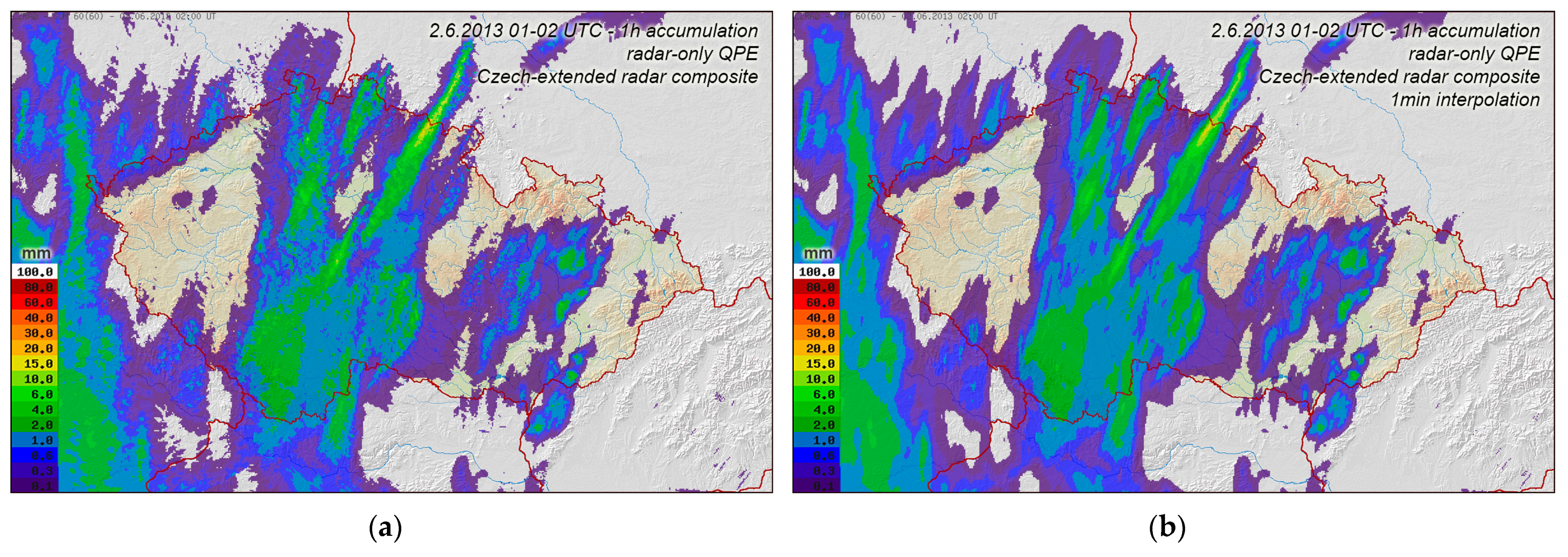
2.1. Radar-Only QPE
- For Z < 7 dBZ, R = 0 mm h–1; threshold condition is used to eliminate weak non-precipitation echoes,
- For Z ≥ 55 dBZ, R = 99.85 mm h–1; threshold condition is applied to reduce rainfall rate overestimation caused by the occurrence of hails in cores of convective storms.
2.2. MERGE2—Combined Radar-Rain Gauge QPE
2.3. Radar-Based QPF
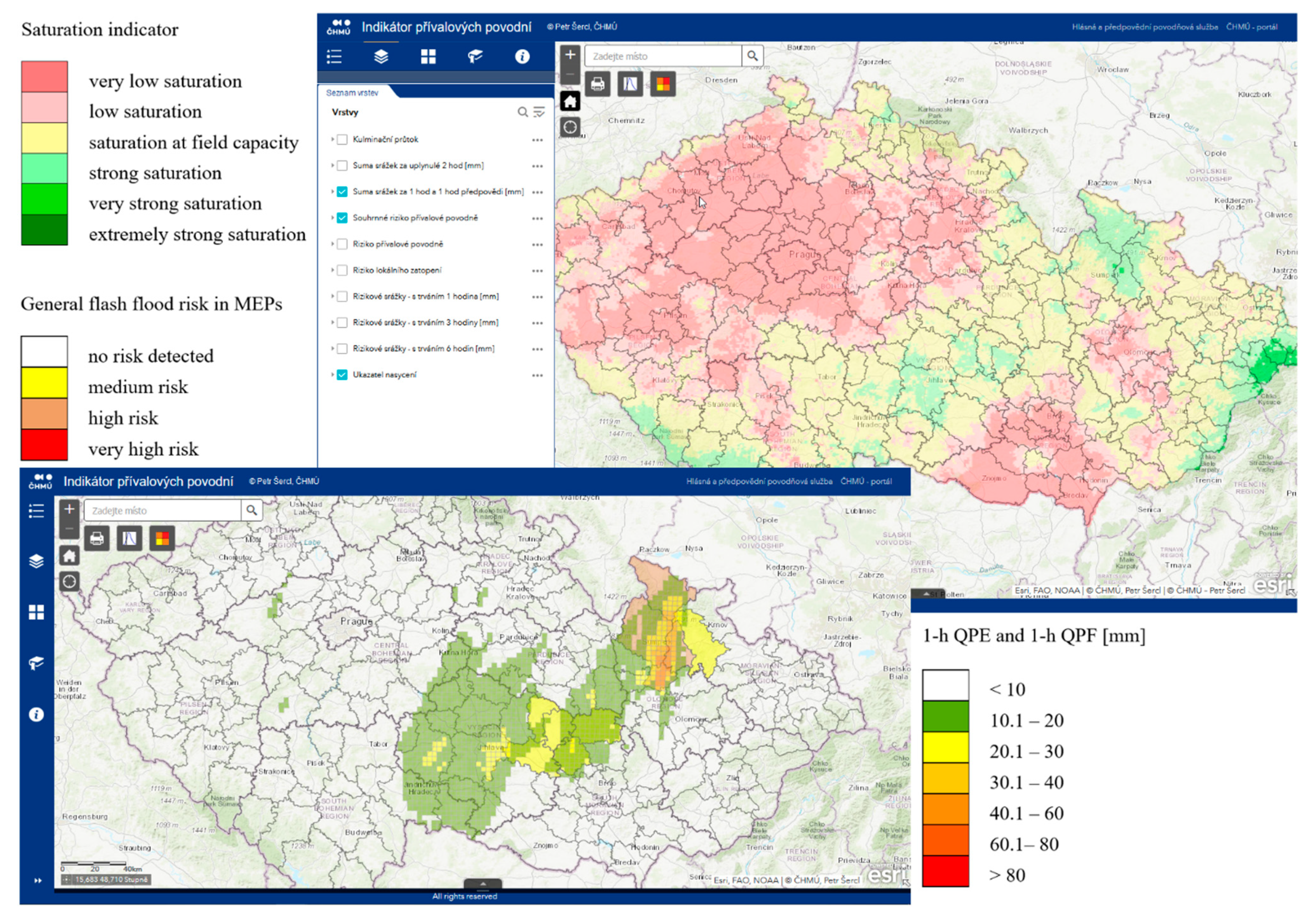
2.4. Flash Flood Indicator
- Calculation of the current soil moisture conditions over an area in a daily step based on the water balance of rainfall, runoff and actual evapotranspiration;
- Calculation of the potential risk rainfall with the durations of 1, 3, and 6 h, which may cause significant surface runoff;
- An estimate of the general flash flood risk based on the 15 min adjusted radar QPE and QPF and defined runoff thresholds. The general flash flood risk is computed as a combination of the local flooding risk for grids with a cell size of 9 km2 and the flash flood risk by using the schematic of hydrologically connected river basins and reaches.
- Run in a daily time step;
- Run in a shorter time step (by configuration).
- Actual data on the soil moisture conditions of the area (represented by CN values), derived from the daily time step of the water balance of the daily rainfall (24 h MERGE QPE), runoff and evapotranspiration, where the main output, is the so-called soil saturation indicator;
- Potential risk amounts of rainfall of a given duration (of 1, 3, and 6 h) for grids with a cell size of 9 km2.
- Level 1—low to medium risk (yellow color), where qmaxi ≥ r1 · q100i;
- Level 2—high risk (orange color), where qmaxi ≥ r2 · q100i;
- Level 3—very high risk (red color), where qmaxi ≥ r3 · q100i.
- Level 1—high rise of water level, flow stays in the river bed, the general public should be informed about the situation;
- Level 2—flow gets out of the river bed locally, mainly not significant damages, the general public should pay increased attention, try to protect its property;
- Level 3—flow gets out of the river bed in many places, significant damages of property, possible loss of life, the general public should be prepared for evacuation.
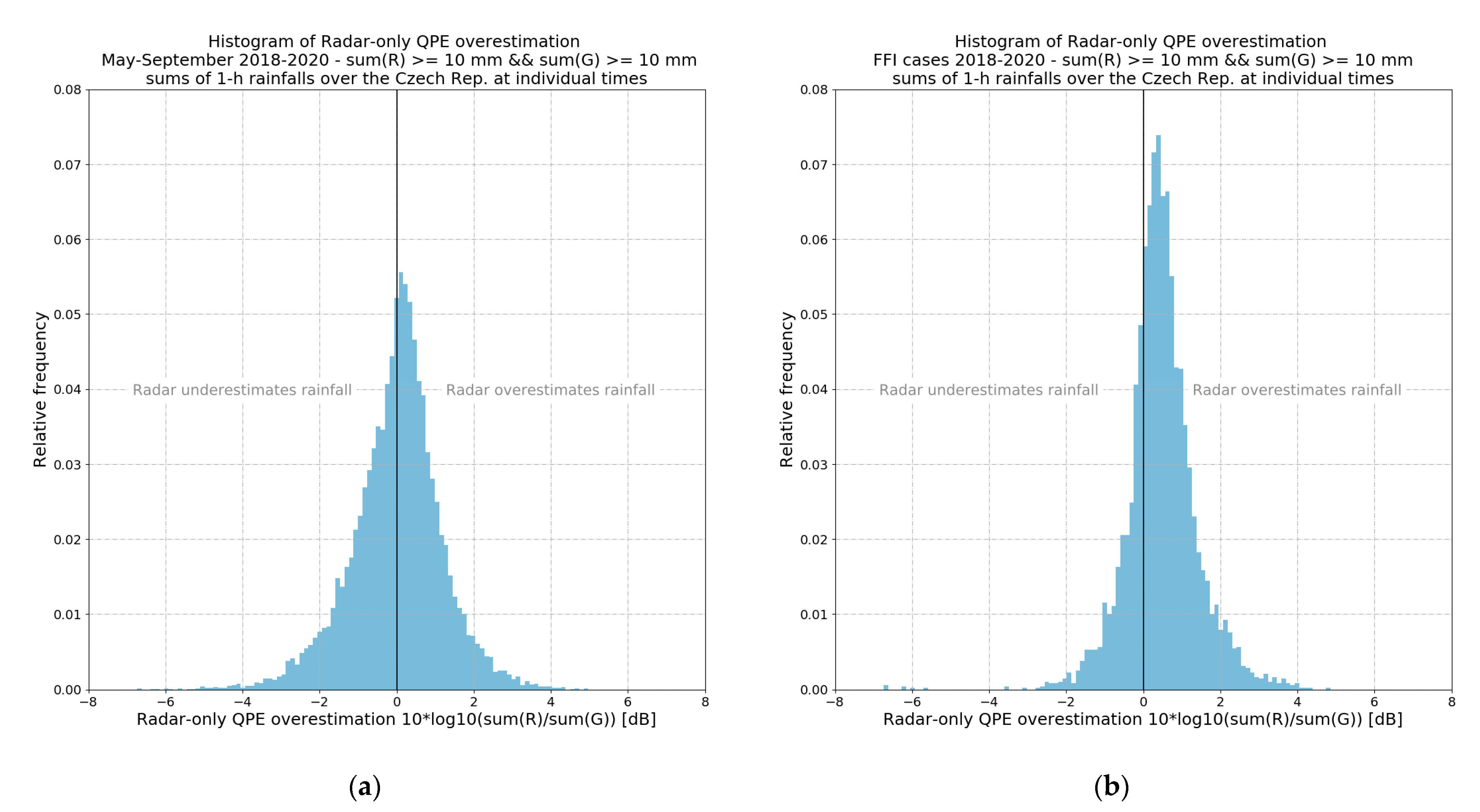
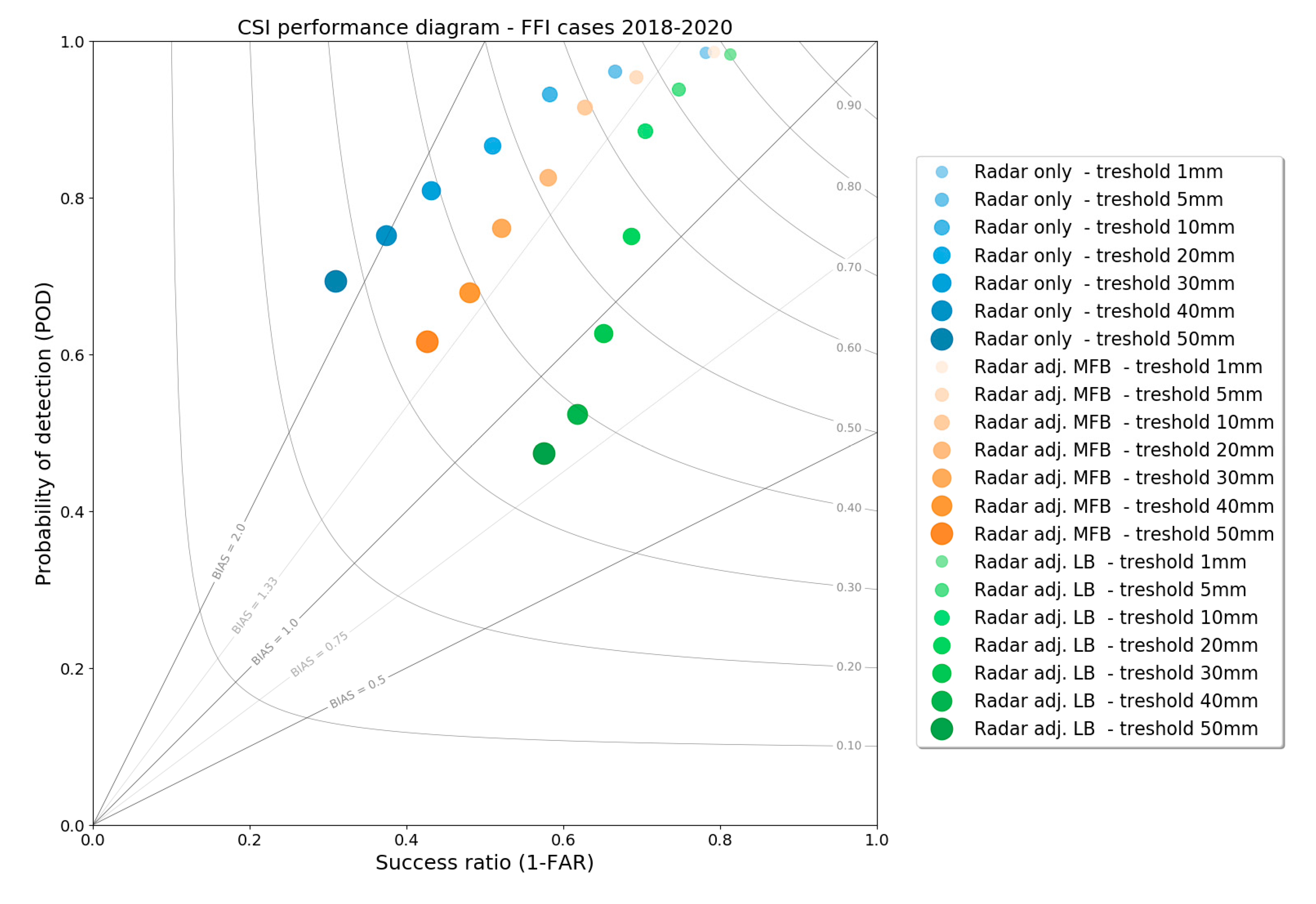
2.5. Performance of Radar-Based QPEs and QPFs in the FFI
- 24 h rainfall have reached or exceeded 10 mm in at least 10 rain gauges during the particular rain event;
- Precipitation was exclusively convective;
- Events with stratiform precipitation, even orographically amplified, were not considered;
- The FFI has detected the flash flood risk or local flooding risk, or there has been direct evidence of a flash flood occurrence.
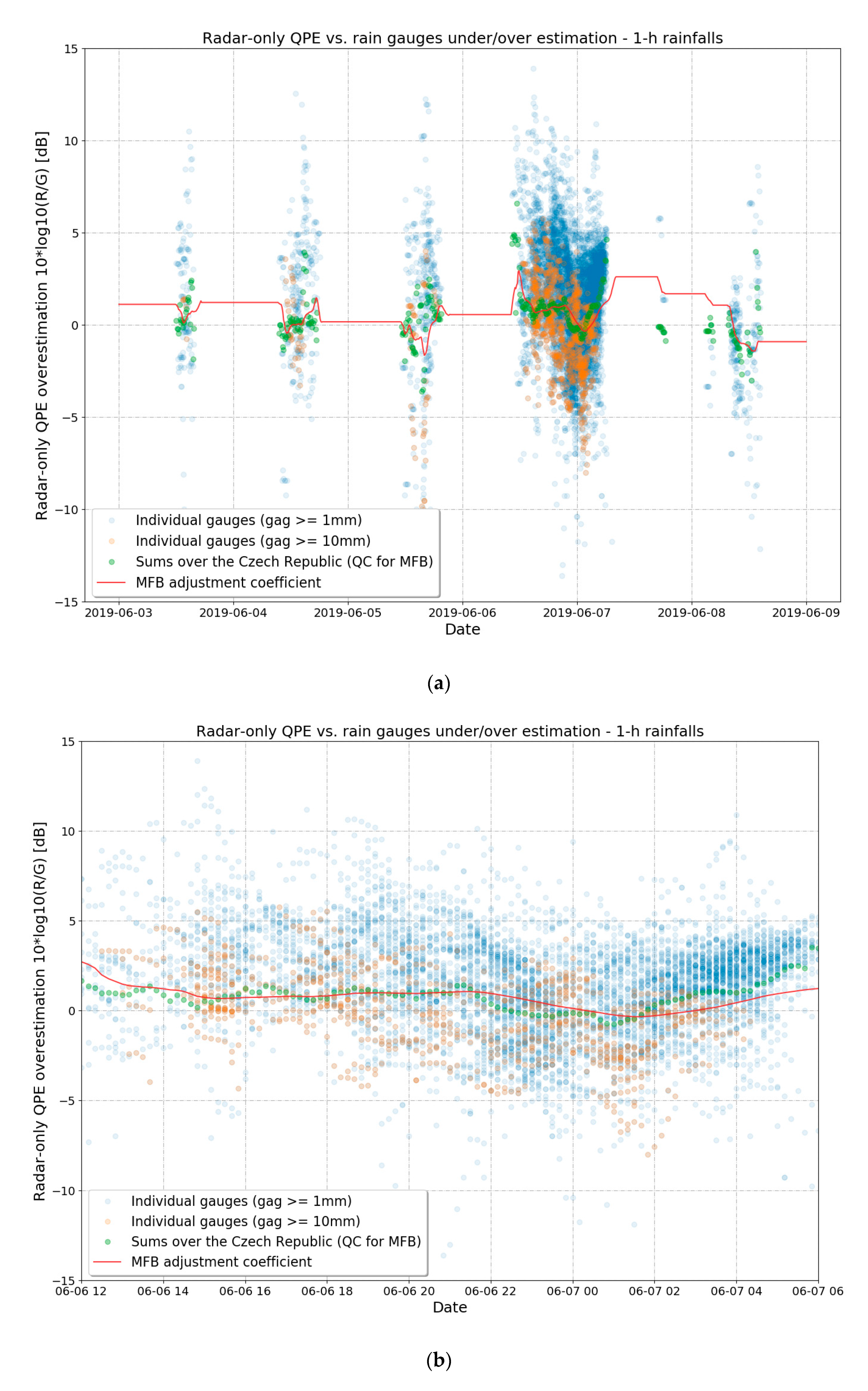
- Conservativeness and robustness of the scalar adjustment coefficient averaged over the whole Czech Republic and the time window;
- Assignment of the corresponding radar-only QPE to the rain gauge measurements for the adjustment coefficient.
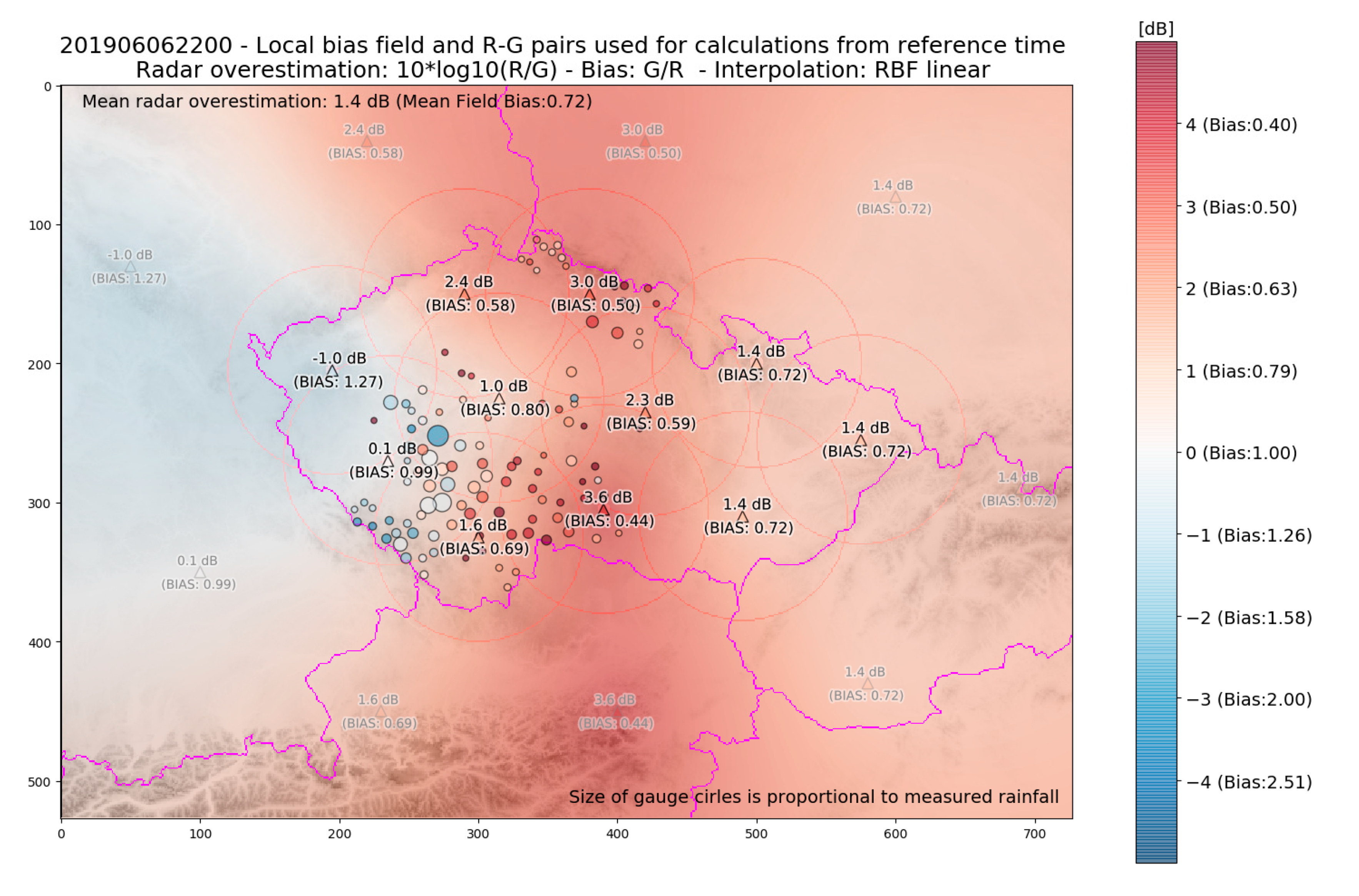
2.6. New Local Bias Adjustment Scheme
- Radar-only QPE at the rain gauge location (instead of the best match from the area of 3 × 3 grid points surrounding the rain gauge) is used to pair the radar-only QPE and the rain gauge measurements;
- Minimum time window from which MFBmod is calculated is 2 h (instead of 3 h);
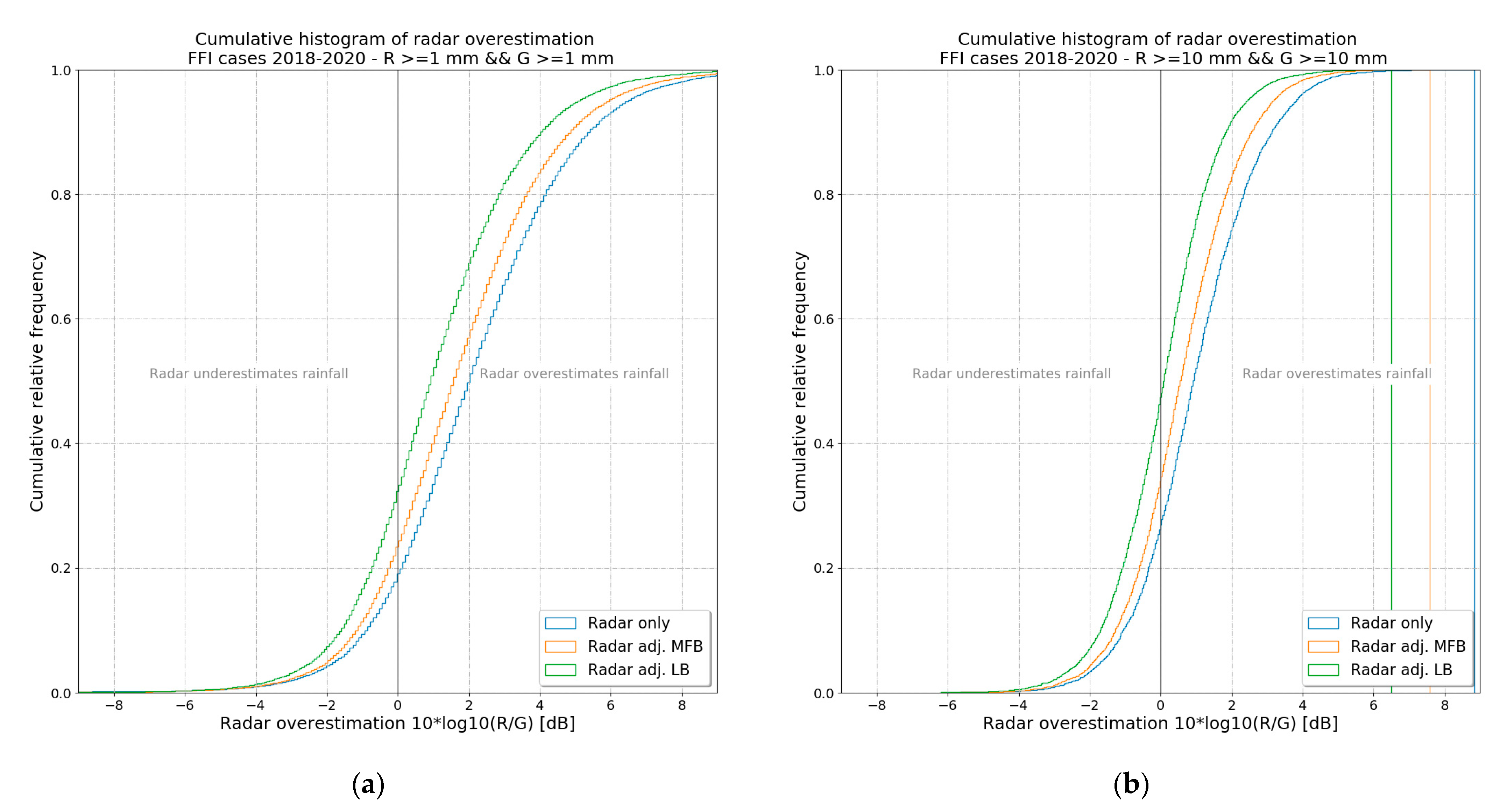
- Default MFBmod value is 0.9 (instead of 1.0 formerly used for MFB). The change of the default value is based on the results shown in Figure 5b. The default MFBmod value is used at the beginning of the precipitation event when it is not possible to accumulate enough precipitation.
3. Results
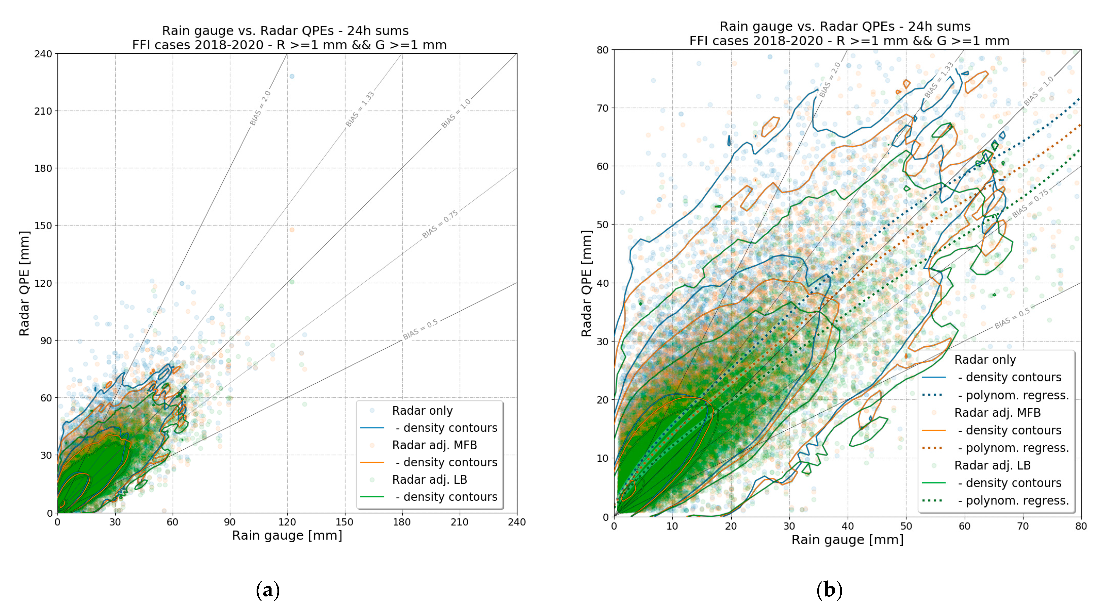
3.1. Statistical Evaluation of the New LB Adjustment Scheme
3.2. Case Studies of the Adjusted Radar QPE Performance as an FFI Input
4. Discussion
5. Conclusions
Author Contributions
Funding
Acknowledgments
Conflicts of Interest
Abbreviations
| ASL | Above sea level |
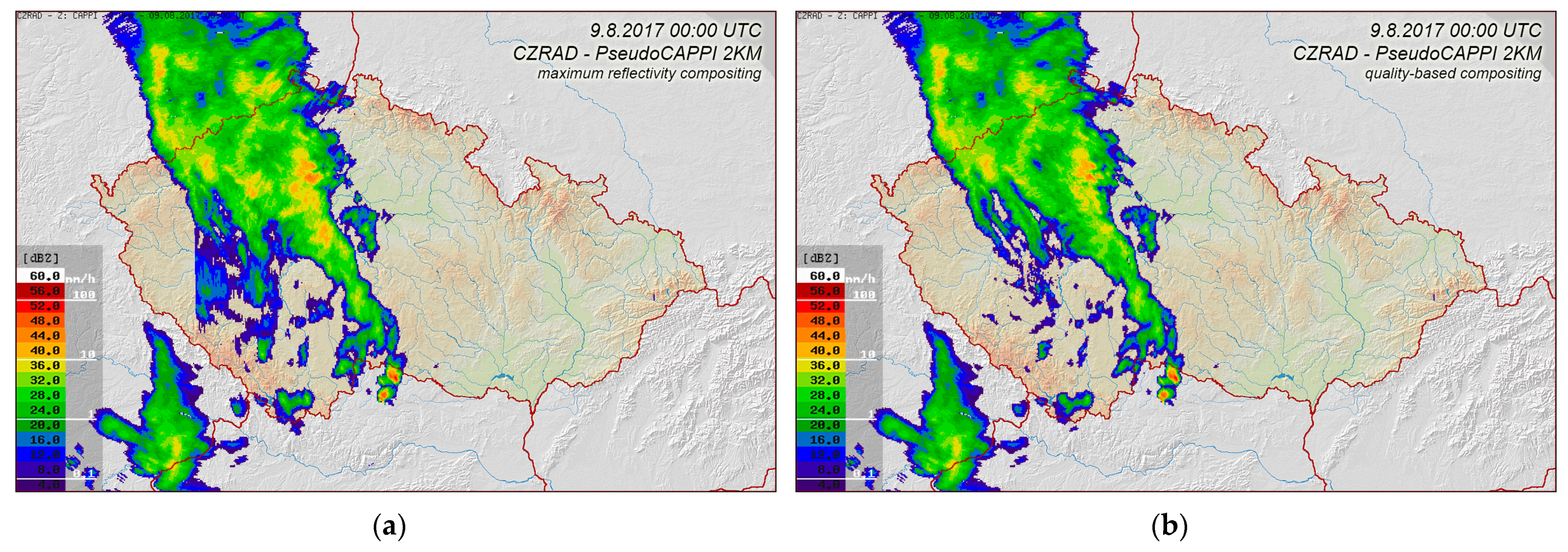
| CAPPI | Constant Altitude Plan Position Indicator |
| CHMI | Czech Hydrometeorological Institute |
| COTREC | Continuity of TREC vectors |
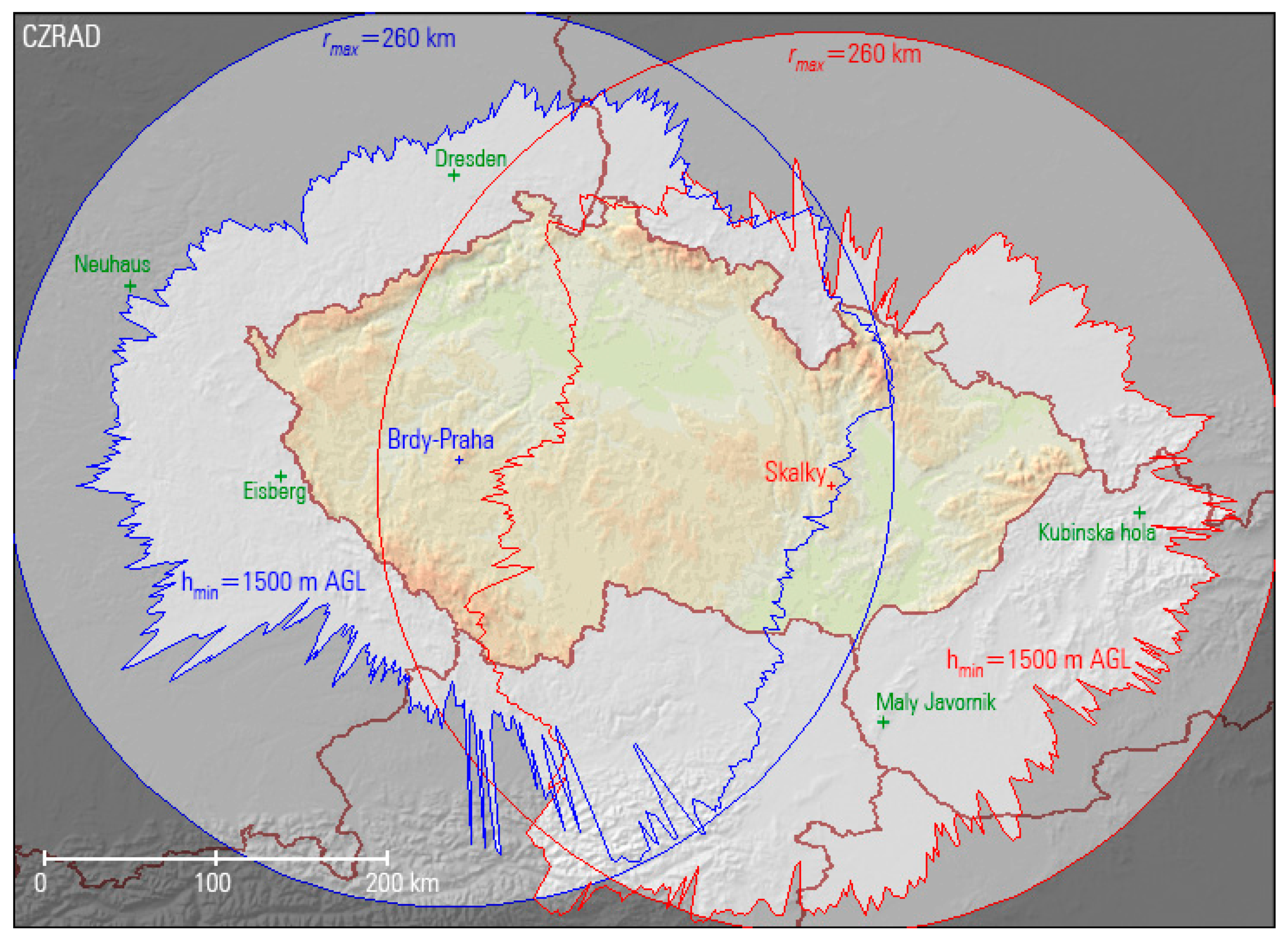
| CZRAD | Czech Weather Radar Network |
| dBZ | Logarithmic unit of radar reflectivity |
| FFI | Flash Flood Indicator |
| LB | Local Bias |
| MAX | Maximum Reflectivity |
| MEP | Municipality with Extended Powers |
| MFB | Mean Field Bias |
| QPE | Quantitative precipitation estimate |
| QPF | Quantitative precipitation forecast |
| SCS-CN | Soil Conservation Service Curve Number |
| VPR | Vertical profile of reflectivity |
| Z-R | conversion from radar reflectivity factor Z to precipitation intensity R |
References
- Novák, P. The Czech hydrometeorological institute’s severe storm nowcasting system. Atmos. Res. 2007, 83, 450–457. [Google Scholar] [CrossRef]
- Novák, P.; Kyznarová, H. Upgrade of the CZRAD meteorological radar network in 2015. Meteorol. Bull. 2016, 69, 137–144. [Google Scholar]
- Šálek, M.; Kráčmar, J. Precipitation estimates by meteorological radar Skalky. Meteorol. Bull. 1997, 50, 99–109. [Google Scholar]
- Šálek, M.; Kráčmar, J.; Novák, P.; Setvák, M. Application of remote sensing methods during the July 1997 floods in the Czech Republic. Meteorol. Bull. 1997, 50, 177–178. [Google Scholar]
- Kráčmar, J.; Joss, J.; Novák, P.; Havránek, P.; Šálek, M. First steps towards quantitative usage of data from weather radar network. In Proceedings of the Final Seminar of COST-75: Advanced Weather Radar Systems, Locarno, Switzerland, 23–27 March 1998; European Commission: Luxembourg, 1999; pp. 91–101, ISBN 9282849074. [Google Scholar]
- Novák, P.; Kráčmar, J. Vertical reflectivity profiles in the Czech Weather Radar Network. In Preprint of Proceedings of 30th International Conference on Radar Meteorology, Munich, Germany, 19–24 July 2001; [CD-ROM, P15.3.]; American Meteorological Society: Boston, MA, USA, 2001. [Google Scholar]
- Šálek, M.; Novák, P.; Seo, D.J. Operational application of combined radar and raingauges precipitation estimation at the CHMI. In Proceedings of the 3rd European Conference on Radar in Meteorology and Hydrology (ERAD 2004), ERAD Publication Series, Visby, Sweden, 6–10 September 2004; Copernicus GmbH: Göttingen, Germany, 2004; Volume 2, pp. 16–20. [Google Scholar]
- Šálek, M. Operational application of the precipitation estimate by radar and raingauges using local bias correction and regression kriging. In Proceedings of the 6th European Conference on Radar in Meteorology and Hydrology (ERAD 2010), Sibiu, Romania, 6–10 September 2010; National Meteorological Administration of Romania: Sibiu, Romania, 2010; pp. 39–43. [Google Scholar]
- Šálek, M. Merging of Weather Radar and Rain Gauge Measurements for Precipitation Estimation. Ph.D. Thesis, Brno University of Technology, Brno, Czech Republic, 2011. [Google Scholar]
- Novák, P.; Kyznarová, H. Progress in operational quantitative precipitation estimation in the Czech Republic. In Proceedings of the 8th European Conference on Radar in Meteorology and Hydrology (ERAD 2014), Garmisch-Partenkirchen, Germany, 1–5 September 2014. QPE.P06. [Google Scholar]
- Novák, P.; Kyznarová, H. MERGE2—the upgraded system of quantitative precipitation estimates operated at the Czech Hydrometeorological Institute. Meteorol. Bull. 2016, 69, 137–144. [Google Scholar]
- Novák, P.; Březková, L.; Frolík, P. Quantitative precipitation forecast using radar echo extrapolation. Atmos. Res. 2009, 93, 328–334. [Google Scholar] [CrossRef]
- Šálek, M.; Březková, L. Utilization of radar-based precipitation estimate in hydrological models in the Czech Republic. In Proceedings of the 3rd European Conference on Radar in Meteorology and Hydrology (ERAD 2004), ERAD Publication Series, Visby, Sweden, 6–10 September 2004; Copernicus GmbH: Göttingen, Germany, 2004; Volume 2, pp. 516–521. [Google Scholar]
- Šálek, M.; Březková, L.; Novák, P. The use of radar in hydrological modelling in the Czech Republic—Case studies of flash floods. Nat. Hazards Earth Syst. Sci. 2006, 6, 229–236. [Google Scholar] [CrossRef]
- Březková, L.; Novák, P.; Šálek, M.; Kyznarová, H.; Jonov, M.; Frolík, P.; Sokol, Z. The operational use of nowcasting methods in hydrological forecasting at the Czech Hydrometeorological Institute. In Weather Radar and Hydrology, Proceedings of the International Symposium, Exeter, UK, 18–21 April 2011; IAHS: Wallingford, UK, 2012; Volume 351, pp. 490–495. ISBN 9781907161261. [Google Scholar]
- Šercl, P. Flash Flood Indicator. Possibilities of prediction of flash floods in the conditions of the Czech Republic. In Transactions of the CHMI; CHMI: Prague, Czech Republic, 2015; Volume 60, pp. 10–28. ISBN 9788087577271. [Google Scholar]
- Šálek, M.; Cheze, J.-L.; Handwerker, J.; Delobbe, L.; Uijlenhoet, R. Radar Techniques for Identifying Precipitation Type and Estimating Quantity of Precipitation; Document of COST Action 717; Office for Official Publications of the European Communities: Luxembourg, 2004; p. 51. ISBN 9289800046. [Google Scholar]
- Overeem, A.; Holleman, I.; Buishand, A. Derivation of a 10-year radar-based climatology and rainfall. J. Appl. Meteorol. Climatol. 2009, 48, 1448–1463. [Google Scholar] [CrossRef]
- Newsome, D.H. Weather radar networking. In Final Report of COST 73 Project; Kluwer Academic Publishers: Dordrecht, The Netherlands, 1992; pp. 41–50. [Google Scholar]
- Kráčmar, J. Radar horizons and the occurrence of ground clutters for weather radar network of the Czech Republic. Meteorol. Bull. 1994, 47, 163–171. [Google Scholar]
- Jurczyk, A.; Szturc, J.; Ośródka, K. Quality-based compositing of weather radar derived precipitation. Meteorol. Appl. 2020, 27, e1812. [Google Scholar] [CrossRef] [Green Version]
- Marshall, J.S.; Palmer, W. McK. The distribution of rain drops with size. J. Meteor. 1948, 5, 165–166. [Google Scholar] [CrossRef]
- Fulton, R.A.; Breidenbach, J.P.; Seo, D.-J.; Miller, D.A.; O’Bannon, T. The WSR-88D rainfall algorithm. Weather Forecast. 1998, 13, 377–395. [Google Scholar] [CrossRef]
- Goudenhoofdt, E.; Delobbe, L. Evaluation of radar-gauge merging methods for quantitative precipitation estimates. Hydrol. Earth Syst. Sci. 2009, 13, 195–203. [Google Scholar] [CrossRef] [Green Version]
- Keller, D. Evaluation and comparison of radar-rain gauge combination methods. In Scientific Report MeteoSwiss; MeteoSwiss: Zürich, Switzerland, 2013; Volume 94. [Google Scholar]
- Li, L.; Schmid, W.; Joss, J. Nowcasting of motion and growth of precipitation with radar over a complex orography. J. Appl. Meteorol. 1995, 34, 1286–1300. [Google Scholar] [CrossRef] [Green Version]
- Zgonc, A.; Rakovec, J. Time extrapolation of radar echo patterns. In Proceedings of the Final Seminar of COST-75: Advanced Weather Radar Systems, Locarno, Switzerland, 23–27 March 1998; European Commission: Luxembourg, 1999; pp. 229–238, ISBN 9282849074. [Google Scholar]
- Šercl, P. The robust method for an estimate of runoff caused by torrential rainfall and proposal of a warning system. In Proceedings of the Early Warning for Flash Floods Workshop, Prague, Czech Republic, 1–2 November 2010; CHMI: Prague, Czech Republic, 2011; pp. 76–81, ISBN 9788086690919. [Google Scholar]
- Mishra, S.K.; Singh, V.P. Soil Conservation Service Curve Number (SCS-CN) Methodology; Springer: Basel, Switzerland, 2003; p. 216. ISBN 9781402011320. [Google Scholar] [CrossRef]
- Janeček, M. Using the CN runoff curve number method to design anti-erosion measures. In Soil Protection against Erosion; Dům Techniky České Budějovice: České Budějovice, Czech Republic, 1998; pp. 1–35. ISBN 9788002012313. [Google Scholar]
- US Army Corps of Engineer. Engineering and Design: Flood-Runoff Analysis (Engineer Manual 1110-2-1417); Military Bookshop: Washington, DC, USA, 1994; p. 228. ISBN 978-1780397474. [Google Scholar]
- Borovička, P. Preventing of Security Hazards Caused by Extreme Meteorological Phenomena—Their Specification and Innovation of Forecasting and Warning Systems with Regards to Climate Change; Final Report on Project VH20172020017; Ministry of the Interior of the Czech Republic: Prague, Czech Republic, 2020; p. 76.
- Šercl, P. Impact of physio-geographical factors on theoretical design flood wave characteristics. In Transactions of the CHMI; CHMI: Prague, Czech Republic, 2009; Volume 54, ISBN 9788086690629. [Google Scholar]
- Flash Flood Indicator in Web Mapping Application. Available online: https://1url.cz/vKEoE (accessed on 2 July 2021).
- CHMI’s Flood Forecasting Service. Available online: https://hydro.chmi.cz/hpps/main_rain.php?mt=ffg (accessed on 2 July 2021).
- ArcGIS Pro Help/RBF (Radial Basis Functions)/How Radial Basis Functions Work. Available online: https://pro.arcgis.com/en/pro-app/latest/help/analysis/geostatistical-analyst/how-radial-basis-functions-work.htm (accessed on 2 July 2021).
- SciPy API Reference—Scipy.interpolate.Rbf. Available online: https://docs.scipy.org/doc/scipy/reference/generated/scipy.interpolate.Rbf.html (accessed on 2 July 2021).
- Roebber, P.J. Visualizing multiple measures of forecast quality. Wea. Forecast. 2009, 24, 601–608. [Google Scholar] [CrossRef] [Green Version]


| Year | Number of Selected Events | Count of Paired Values | Mean Measured 24 h Rainfall [mm] | Mean 24 h Adjusted Radar QPE [mm] | Geometric Mean of Ratios (Adjusted/Measured) |
|---|---|---|---|---|---|
| 2018 | 16 | 888 | 22.4 | 26.0 | 1.13 |
| 2019 | 17 | 1267 | 20.9 | 21.8 | 1.02 |
| 2020 | 22 | 1842 | 20.6 | 22.4 | 1.07 |
| Date | Adjustment Scheme | Risk Level 1 Totals | Risk Level 2 Totals | Risk Level 3 Totals | Risk Totals | Number of Grid Cells |
|---|---|---|---|---|---|---|
| 13 June 2020 | old MFB new LB | 9 11 | 6 6 | 6 6 | 21 23 | 267 242 |
| 18 June 2020 | old MFB new LB | 52 69 | 20 31 | 9 36 | 81 136 | 485 541 |
| 19 June 2020 | old MFB new LB | 0 0 | 0 0 | 0 0 | 0 0 | 153 31 |
| 4 August 2020 | old MFB new LB | 25 0 | 2 0 | 0 0 | 27 0 | 298 44 |
| Date | Adjustment Scheme | Risk Level 1 Totals | Risk Level 2 Totals | Risk Level 3 Totals | Risk Totals | Number of Involved Catchments |
|---|---|---|---|---|---|---|
| 13 June 2020 | old MFB new LB | 14 8 | 5 5 | 1 1 | 20 14 | 28 25 |
| 18 June 2020 | old MFB new LB | 40 87 | 7 16 | 7 7 | 54 110 | 119 153 |
| 19 June 2020 | old MFB new LB | 30 20 | 24 20 | 19 4 | 73 44 | 82 65 |
| 4 August 2020 | old MFB new LB | 39 32 | 55 16 | 34 4 | 128 52 | 139 54 |
Publisher’s Note: MDPI stays neutral with regard to jurisdictional claims in published maps and institutional affiliations. |
© 2021 by the authors. Licensee MDPI, Basel, Switzerland. This article is an open access article distributed under the terms and conditions of the Creative Commons Attribution (CC BY) license (https://creativecommons.org/licenses/by/4.0/).
Share and Cite
Novák, P.; Kyznarová, H.; Pecha, M.; Šercl, P.; Svoboda, V.; Ledvinka, O. Utilization of Weather Radar Data for the Flash Flood Indicator Application in the Czech Republic. Remote Sens. 2021, 13, 3184. https://doi.org/10.3390/rs13163184
Novák P, Kyznarová H, Pecha M, Šercl P, Svoboda V, Ledvinka O. Utilization of Weather Radar Data for the Flash Flood Indicator Application in the Czech Republic. Remote Sensing. 2021; 13(16):3184. https://doi.org/10.3390/rs13163184
Chicago/Turabian StyleNovák, Petr, Hana Kyznarová, Martin Pecha, Petr Šercl, Vojtěch Svoboda, and Ondřej Ledvinka. 2021. "Utilization of Weather Radar Data for the Flash Flood Indicator Application in the Czech Republic" Remote Sensing 13, no. 16: 3184. https://doi.org/10.3390/rs13163184
APA StyleNovák, P., Kyznarová, H., Pecha, M., Šercl, P., Svoboda, V., & Ledvinka, O. (2021). Utilization of Weather Radar Data for the Flash Flood Indicator Application in the Czech Republic. Remote Sensing, 13(16), 3184. https://doi.org/10.3390/rs13163184