Abstract
Urban parks have been proven to cool the surrounding environment, and can thus mitigate the urban heat island to an extent by forming a park cooling island. However, a comprehensive understanding of the mechanism of park cooling islands is still required. Therefore, we studied 32 urban parks in Jinan, China and proposed absolute and relative indicators to depict the detailed features of the park cooling island. High-spatial-resolution GF-2 images were used to obtain the land cover of parks, and Landsat 8 TIR images were used to examine the thermal environment by applying buffer analysis. Linear statistical models were developed to explore the relationships between park characteristics and the park cooling island. The results showed that the average land surface temperature (LST) of urban parks was approximately 3.6 °C lower than that of the study area, with the largest temperature difference of 7.84 °C occurring during summer daytime, while the average park cooling area was approximately 120.68 ha. The park cooling island could be classified into four categories—regular, declined, increased, and others—based on the changing features of the surrounding LSTs. Park area (PA), park perimeter (PP), water area proportion (WAP), and park shape index (PSI) were significantly negatively correlated with the park LST. We also found that WAP, PP, and greenness (characterized by the normalized difference vegetation index (NDVI)) were three important factors that determined the park cooling island. However, the relationship between PA and the park cooling island was complex, as the results indicated that only parks larger than a threshold size (20 ha in our study) would provide a larger cooling effect with the increase in park size. In this case, increasing the NDVI of the parks by planting more vegetation would be a more sustainable and effective solution to form a stronger park cooling island.
1. Introduction
The world is currently experiencing rapid urbanization and industrialization, which has led to dramatic changes in the land use, land cover, and local climatic conditions, thereby exacerbating urban heat island (UHI) effects [1,2,3,4]. The negative effects from UHIs have significantly increased the energy consumption for cooling, physical discomfort, and even death [5,6,7]. It is projected that 60% of the world’s population will live in cities by 2030, and making cities inclusive, safe, resilient, and sustainable is one of the 17 goals proposed by the United Nations to transform our world [8]. In recent years, studies on alleviating the UHI effect have become more popular than its spatial–temporal monitoring [9,10,11,12]. Urban parks, which usually have a combination of blue and green spaces, are among the most important determinants of mitigating UHI effects [13,14,15,16]. Therefore, enhancing the understanding of the cooling effect provided by parks and the drivers of its variations will help in developing policies to mitigate UHI and designing future parks.
Urban parks have been proven to considerably mitigate the UHI because of shading and evaporation effects [17,18,19]. The land surface temperature (LST) of shaded areas is 19 °C lower than that of unshaded areas [17]. Additionally, urban parks cool their surroundings through energy exchange [20]. Several previous studies showed that the average LST of internal urban parks was 1–2 °C, and sometimes 4–8 °C lower than the surroundings, thereby generating a “cooling island” [19,20,21,22,23]. A stronger “cooling island” affects a larger area and provides more outdoor thermal comfort for residents. Consequently, assessing the park cooling island is the most fundamental and important aspect of our study.
One basic question that needs to be solved in relevant studies is the definition of “park cooling island”, or the comprehensive depiction of the cooling effect. Park cooling intensity (PCI) is a commonly used indicator to characterize “cooling islands” [18,23]. In Cao’s study, the PCI was defined as the LST difference between the inside and outside of parks, and the LST outside the park was manually set as the average LST of a 500-m buffer [24]. However, the 500-m buffer may not be applicable to other parks in different study areas. Additionally, other scholars introduced the park cooling distance (PCD) to measure the park cooling island, which is defined as the spatial extent up to which the park could have a significant influence [18,22]. PCD is usually identified using buffer analysis [21]. For instance, the PCD was defined as the distance from the park boundary to the buffer whose LST difference was less than 0.1 °C [25]. The concept of “first turning point” of the LST curve proposed in Peng’s study was used to define the largest cooling distance (or PCD), which was the distance between the park boundary and the first turning point [22]. These two indicators can be treated as absolute features of the park cooling island, such as the absolute temperature difference and the absolute cooling area. However, the surrounding thermal environment of a park changes continuously, and the same PCI might occur at different distances. Additionally, the parks that have the same values of park cooling area (PCA; or the same cooling effect) might have different sizes, and the differences between such parks cannot be measured by simply using absolute indicators. Therefore, relative indicators of the park cooling island—such as the changes in surrounding LST per meter or the cooling effect per unit area of the park—should be considered in assessing the park cooling island from the perspective of spatial accumulation [22].
Park characteristics are vital for urban planning and urban climate studies. Numerous studies have explored the relationship between urban characteristics and urban park cooling islands, and the results showed that the park cooling effect could be affected by the park’s size, shape, type, greenness, and other factors [25,26,27]. However, the park cooling island was mainly characterized by a single indicator of PCI, and the effect of urban park features on the relative indicators of the cooling island is still uncertain. Additionally, the effect of the land use/land cover, especially regarding the configuration of park components, was not fully assessed. A review paper also showed that most studies on cooling effects are subject to a single park, and only few have explored the cooling effects of parks on the surrounding environment [28]. These limitations might be attributed to the high cost of such studies. Fortunately, obtaining detailed characteristics of urban parks is facilitated by the development of high-spatial-resolution remote sensing or LiDAR [29,30]. For instance, even an individual tree can be identified using high-resolution images. The thermal infrared remote sensing image can be used to retrieve the LST for each pixel [31,32]; this helps in analyzing the surrounding thermal environment of a park, which is more convenient than in situ air temperature measurements [33,34,35]. The explanation of the LST and air temperature differences remains rooted, and these are only likely to be predicted by fully coupled surface–atmosphere models [4]. Skin temperature was poorly correlated with both air temperature and apparent temperature [36]. However, several studies showed that the relationship between traditional air temperature and LST is statistically significant [37,38]. Therefore, using remote sensing images to conduct park cooling island studies can obtain robust results.
Considering the insufficiencies mentioned above, and to provide implications for the studies of urban park cooling islands, we selected the case of Jinan city, China to: (1) map the detailed characteristics of urban parks, including their composition and configuration features; (2) analyze the features of the park cooling island by comprehensively proposing and using absolute and relative indicators; and (3) identify the most important urban park characteristics that determine the variations of the urban park cooling island.
2. Data and Methodology
2.1. Study Area and Data Sources
Jinan, the capital of Shandong province, which is in the eastern part of China, serves as the political, economic, cultural, educational, and financial center of the region, and is located to the north of Mount Tai. Jinan is famous for its 72 springs, and is known as the “City of Springs”. Jinan has a warm, temperate, continental monsoon climate zone, with four distinct seasons and sufficient sunshine. According to statistics from the Jinan government, the annual average air temperature of Jinan is 14.2 °C. January is the coldest month, with an average air temperature of 0.2 °C, and the highest temperature was observed in July, with an average air temperature of 28.3 °C. The annual average precipitation is 548.7 mm. By the end of 2019, there were 8.91 million permanent residents in the city. The green coverage rate of the built-up area is 40.7%, and the per capita park green area is only 13.1 m2 based on the statistics from Bureau of Forestry and Landscaping of Jinan. Consequently, building and managing urban parks to maximize their ecosystem services—such as climate regulation and thermal environment improvement—has become an urgent problem. The core of Jinan city was selected as the study area, with a size of 295.49 km2 (Figure 1). There are several mountains in the south of Jinan, and to avoid their effects on the local thermal environment and park cooling islands, we selected 32 urban parks that were not adjacent to them (Figure 1).
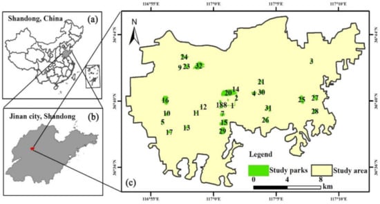
Figure 1.
Location of study area: (a) Shandong province, China; (b) Jinan city in Shandong; (c) study parks in Jinan.
High-spatial-resolution GF-2 images (1 × 1 m) acquired on 4 October 2018, from the Resource and Environmental Science and Data Center, Chinese Academy of Sciences (https://www.resdc.cn/), were used to manually obtain the detailed vector information of urban parks. Three cloud-free Landsat 8 images acquired at about 10:47 a.m. local time for the study area (path 122, row 35, acquired on 17 June 2017-LC81220352017168LGN00, 20 June 2018-LC81220352018171LGN00, and 7 June 2019-LC81220352019158LGN00) were utilized to retrieve the LST, and were obtained from the geospatial data cloud (http://www.gscloud.cn/). Using only one Landsat image may yield an uncertain LST map, as it is subject to the time of satellite overpass. Consequently, the LSTs retrieved from Landsat 8 images acquired over multiple years were averaged to obtain robust results (mean LST) regarding the climate. Data pre-processing (radiometric correction and atmospheric correction) was conducted on the GF-2 and Landsat 8 OLI images prior to the interpretation and LST retrievals.
2.2. Characterizing Urban Parks
The GF-2 images with high spatial resolution facilitated the procurement of detailed information inside a park in this study. Based on the local environment and our prior knowledge, six land cover types (water, trees, shrubs and grass, impervious surfaces, buildings, and bare soil) were extracted by visual interpretation based on image features (e.g., color, size, texture, spatial relationship, etc.). An example of the resulting urban park vector is shown in Figure 2.
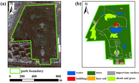
Figure 2.
(a) GF-2 image (true color) of an urban park. (b) Land-cover map of an urban park.
In this research, six widely used landscape metrics and the normalized difference vegetation index (NDVI) (Table 1) were employed to measure the urban park features based on previous studies [21,22], and were classified into two categories: park composition, and park configuration. The composition metrics include the percentage of landscape (PLAND), park area (PA), park perimeter (PP), and the average NDVI of the park (PNDVI). PLAND comprises the water area proportion (WAP), tree area proportion (TAP), shrub and grass area proportion (SGAP), impervious surface area proportion (ISAP), building area proportion (BAP), bare soil area proportion (BSAP), and tree and water area proportion (TWAP). The configurations comprise the park patch density (PPD), park edge density (PED), and park shape index (PSI). These metrics were selected based on previous studies and the following principles: (1) easy calculation and understanding; (2) important in both theory and practice; and (3) comprehensive depiction of urban parks [21,39].

Table 1.
Landscape metrics selected in this study.
2.3. LST Retrieval
The LST was retrieved from Landsat 8 TIRS images. First, the digital number (DN) of band 10 (10.60–11.19 um) was converted into the radiation intensity value using Equation (1) [40]:
where Radiance is the spectral radiance, = the radiance multiplicative scaling factor for band 10, = the radiance additive scaling factor for band 10, and = the level 1 pixel value in DN. All scaling factors can be obtained from the header file.
Subsequently, TIRS data can also be converted from radiance to brightness temperature, which is the effective temperature viewed by the satellite under an assumed emissivity of unity. The conversion formula is as follows:
where T is the top of the atmospheric brightness temperature (Kelvin), and and are conversion constants from the metadata.
Finally, LST can be calculated using Equation (3):
where λ is the wavelength of band 10 (=10.9 µm), α = 1.43 × 10⁻² mK, and ε is the land surface emissivity, which is a crucial variable in the LST retrieval [41]. The calculated LST value (Kelvin) is then converted to °C [31].
In this study, land surfaces’ emissivity was estimated using the NDVI threshold method. NDVI can be calculated using the following equation:
where and represent the atmospherically corrected surface reflectance of bands 5 and 4 for Landsat 8. The land surface emissivity can then be obtained from different NDVI values [42]. If NDVI was greater than 0.5, the land surface emissivity was 0.99, whereas if it was smaller than 0.2, the land surface emissivity was 0.97. In other cases:
where is the vegetation proportion, which can be obtained according to Equation (6):
where = 0.2 and = 0.5.
2.4. Characterizing Park Cooling Island
Urban parks are known to cool their surroundings; however, the cooling effect could decrease with distance from the boundary of the park, and disappear after a certain distance [43]. In previous studies, the urban park cooling island included the following aspects: park cooling intensity (PCI), park cooling distance (PCD), temperature gradient of park cooling gradient (TPCI), park cooling area (PCA), and park cooling efficiency (PCE) [24,25,27,43,44]. In this study, the urban park cooling island was divided into four aspects, as presented in Table 2.
Table 2.
Four aspects of the park cooling island in this study.
As shown in Figure 3a, the surrounding LST increased with increasing distance from the park boundary. Subsequently, the LST curve reached the first turning point, after which the LST changed slightly and even decreased. To characterize the park cooling island, multiple buffer rings (11 in total) with intervals of 90 m at a distance of 990 m from the park boundary were created. Considering that the spatial resolution of the resampled Landsat TIRS is 30 m, the buffer interval was set to 90 m to yield robust results for the LST of each buffer. We assumed that the thermal environment of the latter buffer was not influenced by the urban park if the LST difference between two adjacent buffers was lower than 0.1 °C [21]. Moreover, the distance from the park boundary to the former buffer was defined as the PCD (Figure 3b). The average LST of the buffer with the PCD is treated as the LST of the first turning point, and the area of the buffer is considered to be the PCA. Therefore, the temperature difference between the park and the buffer is the PCI. Consequently, the PCE and PCG can be calculated using the PCA and PCI values.
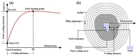
Figure 3.
(a) Illustration of the LST variations. (b) Illustration of the buffer established in this study.
2.5. Statistical Analysis
First, Pearson’s correlation analysis was applied to assess the relationship between the park LST, four aspects of the park cooling island, and its characteristics, in order to examine the landscape metric, showing a significant relationship with the park cooling island. Subsequently, the ordinary least squares linear regression model was used to explore the influence of a single urban park feature on the park cooling island. The four aspects of the park cooling island were the dependent variables, and park features comprised the independent variables. Finally, the different effects of these landscape metrics on the park cooling island were tested using a multiple linear regression model. All statistical analyses were conducted using SPSS software.
3. Results
3.1. Mapping the Characteristics of Urban Parks
A total of 32 urban parks were included in this study. The proportion of land cover types varied among these parks, as shown in Figure 4a. The size of these parks ranged from 2.89 to 107.32 ha, with an average area of 20.81 ha. It can be seen that trees are the most important components of almost every park. Nearly 75% of the parks had a water area. Shrub and grass, together with bare soil, covered a small area in these parks. The configuration landscape metrics and NDVI for each park are shown in Figure 4b. For example, the PSI of these parks ranged from 0.97 to 2.02, with a mean of 1.34, indicating that the shape of parks varied greatly. More detailed statistics of the urban park features are presented in Table 3.
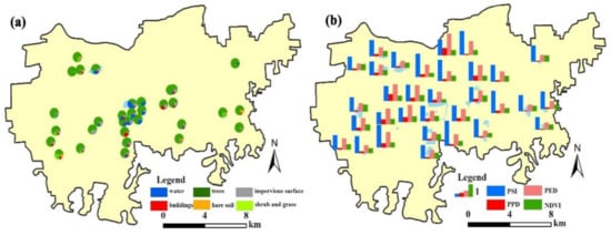
Figure 4.
(a) The proportion of land cover and (b) landscape metrics for each park, respectively.
Table 3.
The statistics of urban park characteristics.
3.2. Characteristics of the Urban Park Cooling Island
The spatial patterns of the average LST are shown in Figure 5a. High LSTs were distributed in the central and eastern parts of the city, where dense buildings and industrial districts exist. Most of the low-LST regions were located in the southern part of the city, with several mountains providing good vegetation coverage as well as a cooling effect. Additionally, the Yellow River in the north generated a “blue cold belt”. The highest, lowest, and mean LST in Jinan city were 48.84, 22.55, and 38.46 °C, respectively. Typically, the LST of urban parks in Jinan city is lower than that of the surrounding areas. The average LST of all 32 parks was 34.86 °C; this was 3.60 °C lower than the average LST of the entire study area, indicating that they provide a cooling effect. Daming Lake Park is a famous scenic area in Jinan city, attracting thousands of residents and tourists each day to enjoy the water and classic garden (Figure 5b1). This area was selected to further illustrate the distribution of the thermal environment. The most important land cover types were water and trees, with area ratios of 48.16 and 36.97%, respectively. This generated a very low-temperature zone inside the park compared to the surrounding areas. As the distance increased from the park boundary (green circle), the color gradually changed from yellow to red, indicating an increase in the LST.
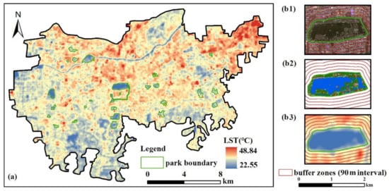
Figure 5.
(a) The distribution of the average LST, (b1) the GF-2 image of Daming Lake Park, (b2) the land cover of Daming Lake Park, and (b3) the LST of Daming Lake Park and its surroundings.
To further compare the different LST and PCI scores among these parks, the average internal LST, corresponding PCI (LST difference between the first turning point and park LST), and largest PCI (defined as the LST difference between the highest LST of all the buffers and park LST) are shown in Figure 6. It can be seen that the average LST in parks varied greatly. For example, park 20 had the lowest internal LST (31.72 °C) and the strongest PCI (7.84 °C), while park 31 had the highest LST (37.42 °C). The largest LST difference among these parks was 5.7 °C. However, the PCI of park 31 (1.46 °C) was larger than that of park 13, whose PCI (0.85 °C) was the weakest. Therefore, the high internal LST of the park did not imply a low PCI, and the PCI was also influenced by its surrounding features. Additionally, the average PCA, PCE, and PCG of these parks were 120.68 ha, 0.71, and 35.45, respectively. The largest PCA, PCE, and PCG were 319.20 ha (park 20), 1.31 (park 20), and 135.28 (park 8), respectively.
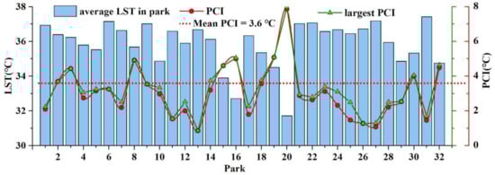
Figure 6.
The internal LST of 32 urban parks and their PCIs.
In this study, a distance of 990 m with 11 buffers (90 m intervals) was established to explore the four aspects of the park cooling island based on the changes in the LST of each buffer. The urban parks were classified into four categories according to the characteristics of the surrounding LST curves: regular parks, declined parks, increased parks, and other parks. As shown in Figure 7a, most parks were regular ones, whose surrounding LST had the following features: a gradual increase in LST with distance from the park boundary, and subsequently reaching the first turning point, after which the LST varied slightly. Seven parks belonged to the second category: declined parks whose surrounding LSTs increased sharply at the beginning and had an obvious decreasing trend after the first turning point. The largest LST difference between the first turning point and the later buffers could reach up to 0.99 °C (park 19), and this value was 0.31 °C for regular parks. For increased parks (Figure 7c), the surrounding LSTs increased from the park boundary to the end of the buffer width and, notably, no decrease in the LSTs was observed. There were also two parks whose surrounding LSTs had no changing features, and these were treated as other parks. In particular, the LST increased sharply from 360 to 630 m for park 8. Moreover, there were several commercial districts with very high LSTs in the buffers, leading to this unusual phenomenon.
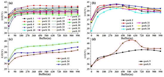
Figure 7.
Variation of surrounding LSTs from the urban park boundary: (a) regular parks, (b) decreased parks, (c) increased parks, and (d) other parks.
3.3. The Effects of Landscape Metrics on the Park Cooling Island
3.3.1. The Relationship between Urban Park Features and LST
Pearson’s correlation analysis was applied to explore the relationships between urban park features and their internal and surrounding LSTs. Only those results of the coefficients that are significant are presented in Table 4. Notably, the internal LST of the parks had negative relationships with PA, PP, and WAP, indicating that large areas and more water bodies could generate a low LST for the parks. The PSI was positively correlated with the park LST. Regarding the relationship between park features and surrounding LSTs, the results showed that the PA had significant positive correlations with the LSTs of all of the buffers. The coefficients gradually decreased from 90 m (R = 0.73) to 450 m (R = 0.56); they subsequently became stronger from 450 to 990 m (R = 0.68). The relationships between PP and surrounding LSTs were not significant from 270 to 540 m, and their positive correlations were weaker compared to those between PA and LSTs. Similarly to PA, WAP had a positive relationship with the LST of all buffers. BAP had negative relationships with the LSTs of buffers between 180 and 450 m, and their correlations were not significant among other buffers.
Table 4.
The correlation coefficients for urban park features and LST.
Based on the results, PA and WAP were seemingly the two most important factors that could affect the park and buffer LSTs. However, the effects of PA and WAP on the park LST were negative, but positive for buffer LSTs. Notably, the park was removed from all buffers, and the LST of buffers did not include park LST.
3.3.2. The Relationship between the Park Features and Park Cooling Island
Based on the results of Section 3.3.1, it can be inferred that large PA and WAP would generate low park LST and high buffer LST. Consequently, this may lead to a strong PCI. Therefore, Pearson’s correlation analysis was initially employed to study the relationships between urban park features and four aspects of park cooling islands. The results of the coefficients are presented in Table 5. PA had positive effects on the PCI (R = 0.58), PCA (R = 0.73), and PCG (R = −0.45), but had negative effects on PCE. The relationship between PP, PCI, and PCG was not significant, and a large PP could lead to a low PCE. In this study, the effect of TAP on PCI was not significant, and differed from other studies wherein trees could improve the park cooling effect. Consistent with expectations, the WAP was positively correlated with the PCI, PCA, and PCG, indicating that more water would produce a better cooling effect.
Table 5.
The correlation coefficients for urban park features and the park cooling island.
To further assess the effects of the two most important factors (PA and WAP) on the park cooling island, simple linear regression models were built for the PA, WAP, and PCI, PCA, PCG, and PCE, respectively. The original result of the linear regression model built for PA and PCI using all of the park samples was not satisfactory, as the adjusted R2 was smaller than 0.30. After exploring the scatter diagram between PCI and PA, a PA threshold (20 ha) was found to divide the parks into two categories. If the PA was smaller than 20 ha (blue points in Figure 8a), the relationship between the PA and PCI was not significant. In this case, the PA had little influence on the PCI. However, if the PA was larger than 20 ha, it had a very strong positive relationship with the PCI. The PCI would increase by 0.7 °C if the PA was 10 ha larger. The threshold of 20 ha for PA was also practical for studying its relationship with the PCA and PCG. Similarly, parks with areas larger than 20 ha had significant positive effects on the PCA and PCG. Regarding the effects of PA on PCE, the latter decreased sharply when PA was smaller than 20 ha, but this rate of decrease was much lower if the PA was larger than 20 ha.
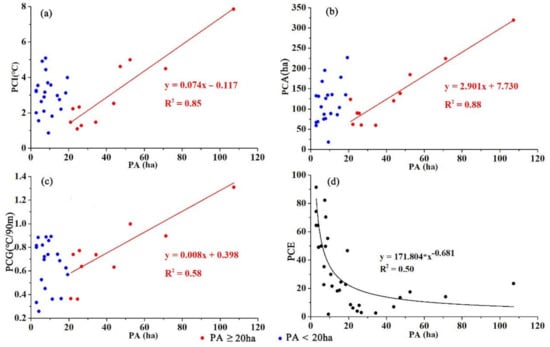
Figure 8.
Linear regression models of the PA and (a) PCI, (b) PCA, (c) PCG, and (d) PCE.
The relationships between WAP and the park cooling island are shown in Figure 9. Typically, water has a strong cooling effect owing to its large specific heat capacity. Consequently, more water in the park would generate an obvious cooling island. In this study, the PCI would increase by 0.89 °C if there were a 10% increase in the WAP. If the PA was larger than 20 ha, the WAP was positively correlated with the PCA. However, the effects of WAP on PCA were not significant if the PA was less than 20 ha. Compared to the PCI and PCA, the relationships between WAP and PCG were much weaker. Our results also showed that no obvious statistical relationships existed between the WAP and PCE. The PCE measures the cooling ability produced per unit area of the park and, thus, WAP was not the dominant factor.
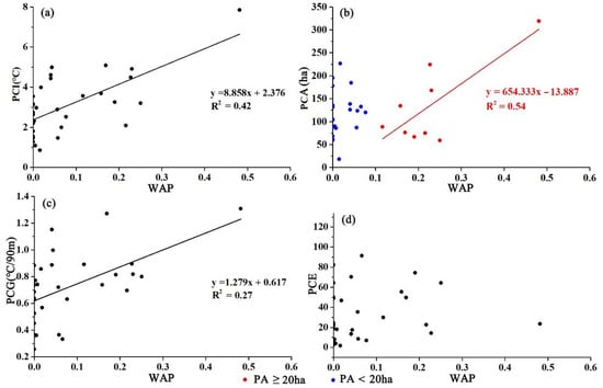
Figure 9.
Linear regression models of the WAP and (a) PCI, (b) PCA, (c) PCG, and (d) PCE.
4. Discussion
4.1. Characterizing the Urban Park Cooling Island
This study demonstrated a park cooling island in Jinan, China. The primary question that needs to be resolved involves understanding the entirety of the park cooling island. In this study, the characteristics of the park cooling island were divided into four aspects—PCI, PCA, PCG, and PCE—based on previous studies and our research [21,22]. PCI and PCA are absolute indicators that reflect the cooling effect of the park as a whole; PCI measures the temperature differences between the park and its surroundings, and the PCA is the largest area whose thermal environment can influence the park. In previous studies, the PCE was used to measure the cooling island [21,27]. However, this is similar to the largest cooling distance in our study, which is a one-dimensional distance. A large and small park may have the same PCE, but the area influenced by the two parks could vary greatly. Consequently, PCA was used instead of PCE in this study. PCG and PCE are different indicators of a park cooling island that measure the relative cooling effect or cooling ability per unit of distance or area. For example, a park with a large area might have a large PCI or PCA but a small PCG or PCE. In our opinion, the four aspects could characterize the park cooling island in a relatively comprehensive manner.
Upon clarifying the ontology of the urban park cooling island, the next question is the method of measuring the park cooling island. In this study, popular Landsat 8 remote sensing images were used to retrieve the LST to characterize the thermal environment. Buffer analysis has proven to be applicable for studying thermal environments [45,46]. However, the different choices of width and interval of buffers could affect and add more uncertainty to the results. Many previous studies used 10–20 buffers, each 30 or 60 m wide [22,27]. As the original spatial resolution of Landsat 8 TIRS was 100 m and resampled to 30 m, 11 buffers with intervals of 90 m were established to identify the cooling distance of the park and determine the PCI and PCA in our study. The total width of these buffers was 990 m, which is larger than that in many previous studies [21,22]. This was because some parks in our cases had a maximum cooling distance of 630 m, and a buffer width of 300 or 450 m could not facilitate the identification of the PCA. Therefore, the methodology used in this study to measure the park cooling islands could provide insights or references for other relevant studies in the future.
4.2. The Effects of Landscape Metrics on the Park LST and Park Cooling Island
During the daytime in summer, our results showed that the park size and WAP had significant negative relationships with the park LSTs. The results were consistent with those of other studies that utilized remote sensing to assess the park cooling island [14,23]. The PSI measures the shape complexity of a park. Our results showed that the coefficient between PSI and park LST was −0.39, indicating that parks with irregular shapes could have lower LSTs, which was in accordance with earlier studies. Other landscapes—such as the PED, PPD, and BAP—had little effect on the park LST. However, other studies showed that the PPD was positively correlated with the park LST, which was not found in this study [21]. This might be attributable to the differences in the studied parks and different climate backgrounds.
The characteristics of the park cooling island are as follows: the average, maximum, and minimum PCIs of the 32 urban parks were 3.60, 7.84, and 0.85 °C, respectively, which is consistent with previous studies [47,48]. Peng’s study showed that the average LST difference between the inside and surrounding of parks was 3.06 °C [22]. Additionally, the average PCA in our study was 120.68 ha, which was much larger than that in Peng’s study (81.3 ha). This might be ascribed to the difference in the buffer interval (30 m in Peng’s study and 90 m in ours). As we proposed a new definition of PCE owing to the limited current literature, it was difficult to compare the PCE to previous studies.
Among the many landscape metrics and features of a park, the dominant factors that determine the park cooling island were further evaluated. Multivariate linear regression models were constructed for this purpose to explore the relative contributions of the variables to the park cooling island. In these models, landscape metrics were independent variables, while PCI, PCA, PCG, and PCE were the dependent variables. The proportion of water was the most important factor in the PCI (Table 5 and Table 6), which is consistent with previous studies [11,49,50,51]. Water helps to reduce LST owing to its large specific heat capacity and the enhanced heat exchange occurring between water and the surrounding environment [52]. Waterbodies are important components of urban parks. However, owing to the accessibility of water resources, increasing the water area in the park to enhance the PCI is unsustainable. The size of the park is another important determining factor in the PCI (Table 5 and Figure 8) [24]. PA had a positive relationship with the PCI, and similar results were also obtained in previous studies [24]. In particular, a large park would produce a strong cooling effect. However, the relationship between the PA and PCI is not a simple linear relationship. Our results showed that almost no correlation existed between the PA and PCI for small parks, with only larger parks leading to stronger PCI for parks larger than a threshold of 20 ha. Similar correlations were also observed between the green space and LST in previous studies [53,54]. The NDVI was the third most important urban feature significantly affecting PCI in our study. The NDVI represents the greenness of the park, and a high NDVI indicates more vegetation [55,56]. Vegetation can reduce the LST through shadows and evapotranspiration, which has been proven by many studies [30,57,58,59]. Consequently, if the PA was smaller than the threshold, increasing the NDVI of parks by adding more vegetation would provide a stronger cooling effect [54]. However, the tree area proportion was not included in the regression model presented in Table 6. One possible reason for this was that in our case, almost all of the parks had relatively high TAP values, and the differences between them were not obvious, thereby not making it a determining factor. This does not imply that trees are not important in urban park planning [28,60]. The PA and WAP also had positive effects on the PCA. Moreover, the effects of the independent variables on the PCG and PCE were not significant, except that the PP had an obvious negative effect on the PCE (Table 6).
Table 6.
Regression results of landscape metrics, NDVI, and PCI, PCA, PCG, and PCE. R2 represents the proportions of the park cooling island variations that can be explained by the model. Colors represent the relative contribution of each metric to variations in the park cooling island. Red and blue represent positive and negative effects, respectively.
Based on our findings, the WAP, PA, and NDVI (greenness) of the park are the three dominant factors that determine the PCI. They deserve more attention in future urban park designs from the perspective of regulating the thermal environment.
4.3. Limitations and Future Research Directions
Our study had several limitations. First, the detailed features of the urban parks were extracted from high-resolution GF-2 images (1 m). However, the inside and surrounding LSTs of parks were of relatively low resolution because of the performance of Landsat 8 TIRS. Simultaneously, the LST data only represent the thermal environment when the satellite transits late in the morning. Temperature is an environmental variable that changes daily. Therefore, finer spatial and temporal resolution LST data acquired by unmanned aerial vehicles equipped with high-performance thermal cameras are expected in future studies. Using both LST and air temperature in the perspective of surface energy balance may generate more comprehensive and robust results to obtain a better understanding of the thermal regime of urban parks [20,61,62]. Second, the number of parks studied was limited, and studying more parks or changing the studied city may yield different results. Third, due to the limited availability of data, the effects of socio-economic factors on park cooling islands were not explored. Future studies can obtain more robust results by applying big data such as the point of interest (POI).
5. Conclusions
To enhance the understanding of the detailed characteristics of the urban park cooling island and the driving mechanisms of its variations, high-spatial-resolution remote sensing images (GF-2) were used to extract the detailed land cover types of urban parks, and landscape metrics were employed to depict the park features. Buffer analysis was conducted to analyze the four aspects of the park cooling island: PCI, PCA, PCG, and PCE. Statistical models were constructed to explore the effects of driving factors on the park cooling island. We found that the average LST of urban parks was approximately 3.60 °C lower than that of the surrounding environment, indicating that parks can provide significant cooling effects. Based on the changing features of surrounding LSTs, the park cooling island could be classified into four categories: regular, increased, decreased, and other parks. Additionally, our results showed that the PA, WAP, and NDVI were the three most important factors that positively affected the park cooling intensity. Theoretically, increasing the waterbody area is the most effective way to enhance the cooling effects of urban parks. However, this might not be a sustainable solution because of the limited water resources, and adding more vegetation to increase the NDVI could prove more feasible. Unfortunately, there was no significant relationship between the PA and PCI if the area was smaller than a threshold of 20 ha in our study. The findings of our study provide valuable insights for the planning and design of urban parks.
Author Contributions
Conceptualization, C.Y.; methodology, W.Z.; software, W.Z.; validation, J.S.; formal analysis, J.S.; investigation, C.Y.; resources, C.J.; data curation, X.X.; writing—original draft preparation, W.Z.; writing—review and editing, C.Y.; visualization, W.Z.; supervision, X.X.; project administration, C.Y.; funding acquisition, M.L. All authors have read and agreed to the published version of the manuscript.
Funding
This research was funded by Shandong Provincial Natural Science Foundation, China, grant number ZR2019BD036, and the Open Fund of Shanghai Key Lab for Urban Ecological Processes and Eco-Restoration, grant number SHUES2021A10.
Institutional Review Board Statement
Not applicable.
Informed Consent Statement
Not applicable.
Conflicts of Interest
The authors declare no conflict of interest.
References
- Arnfield, A.J. Two decades of urban climate research: A review of turbulence, exchanges of energy and water, and the urban heat island. Int. J. Climatol. 2003, 23, 1–26. [Google Scholar] [CrossRef]
- Rizwan, A.M.; Dennis, L.Y.C.; Liu, C. A review on the generation, determination and mitigation of Urban Heat Island. J. Environ. Sci. 2008, 20, 120–128. [Google Scholar] [CrossRef]
- Deilami, K.; Kamruzzaman, M.; Liu, Y. Urban heat island effect: A systematic review of spatio-temporal factors, data, methods, and mitigation measures. Int. J. Appl. Earth Obs. Geoinf. 2018, 67, 30–42. [Google Scholar] [CrossRef]
- Voogt, J.A.; Oke, T.R. Thermal remote sensing of urban climates. Remote Sens. Environ. 2003, 86, 370–384. [Google Scholar] [CrossRef]
- Rizvi, S.H.; Alam, K.; Iqbal, M.J. Spatio -temporal variations in urban heat island and its interaction with heat wave. J. Atmos. Solar Terr. Phys. 2019, 185, 50–57. [Google Scholar] [CrossRef]
- Wong, P.P.-Y.; Lai, P.-C.; Low, C.-T.; Chen, S.; Hart, M. The impact of environmental and human factors on urban heat and microclimate variability. Build. Environ. 2016, 95, 199–208. [Google Scholar] [CrossRef] [Green Version]
- Santamouris, M.; Cartalis, C.; Synnefa, A.; Kolokotsa, D. On the impact of urban heat island and global warming on the power demand and electricity consumption of buildings—A review. Energy Build. 2015, 98, 119–124. [Google Scholar] [CrossRef]
- Bebbington, J.; Unerman, J. Achieving the United Nations sustainable development goals. Account. Audit. Account. J. 2018, 31, 2–24. [Google Scholar] [CrossRef]
- Lehnert, M.; Brabec, M.; Jurek, M.; Tokar, V.; Geletič, J. The role of blue and green infrastructure in thermal sensation in public urban areas: A case study of summer days in four Czech cities. Sustain. Cities Soc. 2021, 66, 102683. [Google Scholar] [CrossRef]
- Cheung, P.K.; Fung, C.K.; Jim, C. Seasonal and meteorological effects on the cooling magnitude of trees in subtropical climate. Build. Environ. 2020, 177, 106911. [Google Scholar] [CrossRef]
- Lin, Y.; Wang, Z.; Jim, C.Y.; Li, J.; Deng, J.; Liu, J. Water as an urban heat sink: Blue infrastructure alleviates urban heat island effect in mega-city agglomeration. J. Clean. Prod. 2020, 262, 121411. [Google Scholar] [CrossRef]
- Lai, D.; Liu, W.; Gan, T.; Liu, K.; Chen, Q. A review of mitigating strategies to improve the thermal environment and thermal comfort in urban outdoor spaces. Sci. Total Environ. 2019, 661, 337–353. [Google Scholar] [CrossRef]
- Akbari, H.; Kolokotsa, D. Three decades of urban heat islands and mitigation technologies research. Energy Build. 2016, 133, 834–842. [Google Scholar] [CrossRef]
- Aram, F.; Solgi, E.; Baghaee, S.; García, E.H.; Mosavi, A.; Band, S.S. How parks provide thermal comfort perception in the metropolitan cores; a case study in Madrid Mediterranean climatic zone. Clim. Risk Manag. 2020, 30, 100245. [Google Scholar] [CrossRef]
- Du, H.; Cai, Y.; Zhou, F.; Jiang, H.; Jiang, W.; Xu, Y. Urban blue-green space planning based on thermal environment simulation: A case study of Shanghai, China. Ecol. Indic. 2019, 106, 105501. [Google Scholar] [CrossRef]
- Chan, S.; Chau, C.; Leung, T. On the study of thermal comfort and perceptions of environmental features in urban parks: A structural equation modeling approach. Build. Environ. 2017, 122, 171–183. [Google Scholar] [CrossRef]
- Vidrih, B.; Medved, S. Multiparametric model of urban park cooling island. Urban For. Urban Green. 2013, 12, 220–229. [Google Scholar] [CrossRef]
- Chang, C.-R.; Li, M.-H. Effects of urban parks on the local urban thermal environment. Urban For. Urban Green. 2014, 13, 672–681. [Google Scholar] [CrossRef]
- Xu, M.; Hong, B.; Mi, J.; Yan, S. Outdoor thermal comfort in an urban park during winter in cold regions of China. Sustain. Cities Soc. 2018, 43, 208–220. [Google Scholar] [CrossRef]
- Spronken-Smith, R.A.; Oke, T.R. The thermal regime of urban parks in two cities with different summer climates. Int. J. Remote Sens. 1998, 19, 2085–2104. [Google Scholar] [CrossRef]
- Yang, C.; He, X.; Yu, L.; Yang, J.; Yan, F.; Bu, K.; Chang, L.; Zhang, S. The Cooling Effect of Urban Parks and Its Monthly Variations in a Snow Climate City. Remote Sens. 2017, 9, 1066. [Google Scholar] [CrossRef] [Green Version]
- Peng, J.; Dan, Y.; Qiao, R.; Liu, Y.; Dong, J.; Wu, J. How to quantify the cooling effect of urban parks? Linking maximum and accumulation perspectives. Remote Sens. Environ. 2021, 252, 112135. [Google Scholar] [CrossRef]
- Chen, X.; Su, Y.; Li, D.; Huang, G.; Chen, W.; Chen, S. Study on the cooling effects of urban parks on surrounding environments using Landsat TM data: A case study in Guangzhou, southern China. Int. J. Remote Sens. 2012, 33, 5889–5914. [Google Scholar] [CrossRef]
- Cao, X.; Onishi, A.; Chen, J.; Imura, H. Quantifying the cool island intensity of urban parks using ASTER and IKONOS data. Landsc. Urban Plan. 2010, 96, 224–231. [Google Scholar] [CrossRef]
- Toparlar, Y.; Blocken, B.; Maiheu, B.; Heijst, G.V. The effect of an urban park on the microclimate in its vicinity: A case study for Antwerp, Belgium. Int. J. Climatol. 2018, 38, e303–e322. [Google Scholar] [CrossRef]
- Sodoudi, S.; Zhang, H.; Chi, X.; Müller, F.; Li, H. The influence of spatial configuration of green areas on microclimate and thermal comfort. Urban For. Urban Green. 2018, 34, 85–96. [Google Scholar] [CrossRef]
- Feyisa, G.L.; Dons, K.; Meilby, H. Efficiency of parks in mitigating urban heat island effect: An example from Addis Ababa. Landsc. Urban Plan. 2014, 123, 87–95. [Google Scholar] [CrossRef]
- Bowler, D.E.; Buyung-Ali, L.; Knight, T.M.; Pullin, A.S. Urban greening to cool towns and cities: A systematic review of the empirical evidence. Landsc. Urban Plan. 2010, 97, 147–155. [Google Scholar] [CrossRef]
- Chen, J.; Jin, S.; Du, P. Roles of horizontal and vertical tree canopy structure in mitigating daytime and nighttime urban heat island effects. Int. J. Appl. Earth Obs. Geoinf. 2020, 89, 102060. [Google Scholar] [CrossRef]
- Bartesaghi-Koc, C.; Osmond, P.; Peters, A. Mapping and classifying green infrastructure typologies for climate-related studies based on remote sensing data. Urban For. Urban Green. 2019, 37, 154–167. [Google Scholar] [CrossRef]
- Ranagalage, M.; Murayama, Y.; Dissanayake, D.; Simwanda, M. The Impacts of Landscape Changes on Annual Mean Land Surface Temperature in the Tropical Mountain City of Sri Lanka: A Case Study of Nuwara Eliya (1996–2017). Sustainability 2019, 11, 5517. [Google Scholar] [CrossRef] [Green Version]
- Dissanayake, D. Land Use Change and Its Impacts on Land Surface Temperature in Galle City, Sri Lanka. Climate 2020, 8, 65. [Google Scholar] [CrossRef]
- Bahi, H.; Mastouri, H.; Radoine, H. Review of methods for retrieving urban heat islands. Mater. Today Proc. 2020, 27, 3004–3009. [Google Scholar] [CrossRef]
- Weng, Q. Thermal infrared remote sensing for urban climate and environmental studies: Methods, applications, and trends. ISPRS J. Photogramm. Remote Sens. 2009, 64, 335–344. [Google Scholar] [CrossRef]
- Mohajerani, A.; Bakaric, J.; Jeffrey-Bailey, T. The urban heat island effect, its causes, and mitigation, with reference to the thermal properties of asphalt concrete. J. Environ. Manag. 2017, 197, 522–538. [Google Scholar] [CrossRef] [PubMed]
- Ho, H.C.; Knudby, A.; Xu, Y.; Hodul, M.; Aminipouri, M. A comparison of urban heat islands mapped using skin temperature, air temperature, and apparent temperature (Humidex), for the greater Vancouver area. Sci. Total Environ. 2016, 544, 929–938. [Google Scholar] [CrossRef] [PubMed]
- Yang, C.; Yan, F.; Zhang, S. Comparison of land surface and air temperatures for quantifying summer and winter urban heat island in a snow climate city. J. Environ. Manag. 2020, 265, 110563. [Google Scholar] [CrossRef] [PubMed]
- Schwarz, N.; Schlink, U.; Franck, U.; Großmann, K. Relationship of land surface and air temperatures and its implications for quantifying urban heat island indicators—An application for the city of Leipzig (Germany). Ecol. Indic. 2012, 18, 693–704. [Google Scholar] [CrossRef]
- Xiao, X.D.; Dong, L.; Yan, H.; Yang, N.; Xiong, Y. The influence of the spatial characteristics of urban green space on the urban heat island effect in Suzhou Industrial Park. Sustain. Cities Soc. 2018, 40, 428–439. [Google Scholar] [CrossRef]
- USGS. Landsat 8 Hand Book. 2016. Available online: https://www.usgs.gov/media/files/landsat-8-data-users-handbook (accessed on 22 June 2021).
- Sobrino, J.A.; Jimenez-Munoz, J.C.; Soria, G.; Romaguera, M.; Guanter, L.; Moreno, J.; Plaza, A.; Martinez, P. Land Surface Emissivity Retrieval From Different VNIR and TIR Sensors. IEEE Trans. Geosci. Remote Sens. 2008, 46, 316–327. [Google Scholar] [CrossRef]
- Sobrino, J.A.; Jiménez-Muñoz, J.C.; Paolini, L. Land surface temperature retrieval from LANDSAT TM 5. Remote Sens. Environ. 2004, 90, 434–440. [Google Scholar] [CrossRef]
- Lin, W.; Yu, T.; Chang, X.; Wu, W.; Zhang, Y. Calculating cooling extents of green parks using remote sensing: Method and test. Landsc. Urban Plan. 2015, 134, 66–75. [Google Scholar] [CrossRef]
- Dai, Z.; Guldmann, J.-M.; Hu, Y. Spatial regression models of park and land-use impacts on the urban heat island in central Beijing. Sci. Total Environ. 2018, 626, 1136–1147. [Google Scholar] [CrossRef] [PubMed]
- Zhao, Z.-Q.; He, B.-J.; Li, L.-G.; Wang, H.-B.; Darko, A. Profile and concentric zonal analysis of relationships between land use/land cover and land surface temperature: Case study of Shenyang, China. Energy Build. 2017, 155, 282–295. [Google Scholar] [CrossRef]
- Dong, J.; Lin, M.; Zuo, J.; Lin, T.; Liu, J.; Sun, C.; Luo, J. Quantitative study on the cooling effect of green roofs in a high-density urban Area—A case study of Xiamen, China. J. Clean. Prod. 2020, 255, 120152. [Google Scholar] [CrossRef]
- Yu, Z.; Yang, G.; Zuo, S.; Jørgensen, G.; Koga, M.; Vejre, H. Critical review on the cooling effect of urban blue-green space: A threshold-size perspective. Urban For. Urban Green. 2020, 49, 126630. [Google Scholar] [CrossRef]
- Kim, G.; Coseo, P. Urban Park Systems to Support Sustainability: The Role of Urban Park Systems in Hot Arid Urban Climates. Forests 2018, 9, 439. [Google Scholar] [CrossRef] [Green Version]
- Hathway, E.A.; Sharples, S. The interaction of rivers and urban form in mitigating the Urban Heat Island effect: A UK case study. Build. Environ. 2012, 58, 14–22. [Google Scholar] [CrossRef] [Green Version]
- Peng, J.; Liu, Q.; Xu, Z.; Lyu, D.; Du, Y.; Qiao, R.; Wu, J. How to effectively mitigate urban heat island effect? A perspective of waterbody patch size threshold. Landsc. Urban Plan. 2020, 202, 103873. [Google Scholar] [CrossRef]
- Yang, G.; Yu, Z.; Jørgensen, G.; Vejre, H. How can urban blue-green space be planned for climate adaption in high-latitude cities? A seasonal perspective. Sustain. Cities Soc. 2020, 53, 101932. [Google Scholar] [CrossRef]
- Ampatzidis, P.; Kershaw, T. A review of the impact of blue space on the urban microclimate. Sci. Total Environ. 2020, 730, 139068. [Google Scholar] [CrossRef] [PubMed]
- Yu, Z.; Guo, X.; Jørgensen, G.; Vejre, H. How can urban green spaces be planned for climate adaptation in subtropical cities? Ecol. Indic. 2017, 82, 152–162. [Google Scholar] [CrossRef]
- Shah, A.; Garg, A.; Mishra, V. Quantifying the local cooling effects of urban green spaces: Evidence from Bengaluru, India. Landsc. Urban Plan. 2021, 209, 104043. [Google Scholar] [CrossRef]
- Alexander, C. Normalised difference spectral indices and urban land cover as indicators of land surface temperature (LST). Int. J. Appl. Earth Obs. Geoinf. 2020, 86, 102013. [Google Scholar] [CrossRef]
- Yuan, F.; Bauer, M.E. Comparison of impervious surface area and normalized difference vegetation index as indicators of surface urban heat island effects in Landsat imagery. Remote Sens. Environ. 2007, 106, 375–386. [Google Scholar] [CrossRef]
- Bartesaghi-Koc, C.; Osmond, P.; Peters, A. Quantifying the seasonal cooling capacity of ‘green infrastructure types’ (GITs): An approach to assess and mitigate surface urban heat island in Sydney, Australia. Landsc. Urban Plan. 2020, 203, 103893. [Google Scholar] [CrossRef]
- Massetti, L.; Petralli, M.; Napoli, M.; Brandani, G.; Orlandini, S.; Pearlmutter, D. Effects of deciduous shade trees on surface temperature and pedestrian thermal stress during summer and autumn. Int. J. Biometeorol. 2019, 63, 467–479. [Google Scholar] [CrossRef] [PubMed]
- Ren, Z.; Zhao, H.; Fu, Y.; Xiao, L.; Dong, Y. Effects of urban street trees on human thermal comfort and physiological indices: A case study in Changchun city, China. J. For. Res. 2021. [Google Scholar] [CrossRef]
- Pamukcu-Albers, P.; Ugolini, F.; La Rosa, D.; Grădinaru, S.R.; Azevedo, J.C.; Wu, J. Building green infrastructure to enhance urban resilience to climate change and pandemics. Landsc. Ecol. 2021. [Google Scholar] [CrossRef]
- Spronken-Smith, R.A.; Oke, T.R.; Lowry, W.P. Advection and the surface energy balance across an irrigated urban park. Int. J. Climatol. 2000, 20, 1033–1047. [Google Scholar] [CrossRef]
- Spronken-Smith, R.A.; Oke, T.R. Scale Modelling of Nocturnal Cooling in Urban Parks. Bound. Layer Meteorol. 1999, 93, 287–312. [Google Scholar] [CrossRef]

Publisher’s Note: MDPI stays neutral with regard to jurisdictional claims in published maps and institutional affiliations. |
© 2021 by the authors. Licensee MDPI, Basel, Switzerland. This article is an open access article distributed under the terms and conditions of the Creative Commons Attribution (CC BY) license (https://creativecommons.org/licenses/by/4.0/).