Abstract
Volcanic ash clouds can damage aircrafts during flight and, thus, have the potential to disrupt air traffic on a large scale, making their detection and monitoring necessary. The new retrieval algorithm VACOS (Volcanic Ash Cloud properties Obtained from SEVIRI) using the geostationary instrument MSG/SEVIRI and artificial neural networks is introduced in a companion paper. It performs pixelwise classifications and retrieves (indirectly) the mass column concentration, the cloud top height and the effective particle radius. VACOS is comprehensively validated using simulated test data, CALIOP retrievals, lidar and in situ data from aircraft campaigns of the DLR and the FAAM, as well as volcanic ash transport and dispersion multi model multi source term ensemble predictions. Specifically, emissions of the eruptions of Eyjafjallajökull (2010) and Puyehue-Cordón Caulle (2011) are considered. For ash loads larger than 0.2 g m−2 and a mass column concentration-based detection procedure, the different evaluations give probabilities of detection between 70% and more than 90% at false alarm rates of the order of 0.3–3%. For the simulated test data, the retrieval of the mass load has a mean absolute percentage error of ~40% or less for ash layers with an optical thickness at 10.8 μm of 0.1 (i.e., a mass load of about 0.3–0.7 g m−2, depending on the ash type) or more, the ash cloud top height has an error of up to 10% for ash layers above 5 km, and the effective radius has an error of up to 35% for radii of 0.6–6 μm. The retrieval error increases with decreasing ash cloud thickness and top height. VACOS is applicable even for overlaying meteorological clouds, for example, the mean absolute percentage error of the optical depth at 10.8 μm increases by only up to ~30%. Viewing zenith angles >60° increase the mean percentage error by up to ~20%. Desert surfaces are another source of error. Varying geometrical ash layer thicknesses and the occurrence of multiple layers can introduce an additional error of about 30% for the mass load and 5% for the cloud top height. For the CALIOP data, comparisons with its predecessor VADUGS (operationally used by the DWD) show that VACOS is more robust, with retrieval errors of mass load and ash cloud top height reduced by >10% and >50%, respectively. Using the model data indicates an increase in detection rate in the order of 30% and more. The reliability under a wide spectrum of atmospheric conditions and volcanic ash types make VACOS a suitable tool for scientific studies and air traffic applications related to volcanic ash clouds.
1. Introduction
A new volcanic ash retrieval using artificial neural networks (ANNs) and the Spinning Enhanced Visible and Infrared Imager (SEVIRI) aboard the Meteosat Second Generation (MSG) satellites is developed and presented; this algorithm is called VACOS (Volcanic Ash Cloud Properties Obtained from SEVIRI) and builds upon its predecessor VADUGS (Volcanic Ash Detection Using Geostationry Satellites [1]). The companion paper [2] describes the algorithm development: Using a comprehensive set of volcanic ash optical properties [3], surface emissivities [4,5,6] and atmospheric profiles of pressure, temperature, air density, concentrations of oxygen, water vapor, ozone, carbon dioxide and nitrogen dioxide, liquid and ice water clouds, mostly derived from ECMWF model reanalyses, one-dimensional radiative transfer calculations are performed with and without realistic volcanic ash clouds to create training, validation and test data sets. These three simulated data sets contain the volcanic ash cloud properties, i.e., geometrical vertical extent, mass volume concentration, cloud top height, the brightness temperatures (BTs) of the infrared channels of SEVIRI and various auxiliary quantities. The ash-free simulations are validated by comparing the results of radiative transfer calculations of a specific date with the corresponding SEVIRI measurements. Using the simulated data sets, four different ANNs are trained for the pixelwise retrieval of the optical depth at 10.8 μm due to ash (), the ash cloud top height (in , ), the effective particle radius (in , ) and an overall classification in four categories (ash-free and cloud-free; only meteorological clouds; only volcanic ash clouds; both volcanic ash and meteorological clouds present). The ANN for classification returns a normalized four-dimensional vector, where each component can be roughly interpreted as the probability of the corresponding category. The four ANNs perform independently of each other, but the retrievals of and receive an estimate of as an input. This approach allowed to use different training data sets and ANN settings for each retrieval.
This paper contains an analysis of the retrieval performance: A detailed validation with respect to simulated test data sets is presented (Section 2) and the sensitivity of the retrievals with respect to the volcanic ash cloud profile is given (Section 3). To demonstrate the reliability of the new algorithm and to check its performance with respect to its predecessor, various comparisons with other remote and in situ measurements (Section 4) and model calculations were made (Section 5). The individual features of the final ANNs are analyzed to make some inferences on the functioning of the algorithms (Section 6). Finally, we give a conclusion and an outlook.
2. Performance on Simulated Test Data
The development of the VACOS retrieval is described in Piontek et al. [2]. In the following, we systematically quantify the performance of the retrievals with respect to volcanic ash cloud properties, presence of meteorological clouds (defined to include liquid and ice water clouds) and geographic location. Therefore, the ANNs are applied to the test data sets A (1,252,470 samples) or B (405,556 samples) from Piontek et al. [2], depending on their training data set. The samples of the test data sets are the results of independent radiative transfer calculations and can be compared to the situation for single pixels in a SEVIRI image. The VACOS results are compared with these true values, providing references for the error of the retrievals; those might be larger in reality due to more complicated atmospheric conditions (e.g., additional aerosols such as mineral dust), cases that have not been covered by the training data set (e.g., non-homogeneous ash clouds or multiple ash layers, emitted sulfur dioxide) or slight differences between our radiative transfer calculations and the reality (e.g., due to partial cloud covers, inaccuracies due to the applied parameterizations for meteorological clouds). The error metrics mean absolute percentage error (MAPE), mean percentage error (MPE), probability of detection (POD), false alarm rate (FAR) and accuracy are used and described in Appendix A.
2.1. Classification
The classification ANN returns a normalized four-dimensional vector with each component interpreted as the probability of the corresponding category, see Table 1. Defining that a sample is assigned to a given category if the corresponding component is >50%, the accuracy is 92% with 0.012% of the samples remaining unclassified. These values depend on the composition of the test data set with respect to the different categories, as they are retrieved with different accuracy, see Table 1. Whereas clear sky, cloudy and ash-loaded samples are correctly classified with probabilities of more than 90% each, samples with both meteorological and ash clouds are correctly classified in only 49% of the cases. About 47% of those samples were classified as ash only. Again, this might depend on the composition of the test data; samples with thick ash clouds on top of comparably thin meteorological clouds might be misclassified as ash only. Reducing the amount of these samples in the test data set would significantly modify the results in Table 1. Nevertheless, VACOS is able to detect the presence of ash in almost all cases even for this category, with only 4.1% of the ash remaining undetected. Next, only the samples containing ash and meteorological clouds are considered and separated according to the location of the meteorological clouds as above or below the ash layer, where we define that above denotes that no meteorological clouds are below the volcanic ash cloud bottom and below that no meteorological cloud is above the ash cloud top. Samples with multiple meteorological clouds located both above and below the ash layer are not included in either class. Again, note that we do not differentiate between liquid and ice water clouds, although ice water clouds can be expected to dominate for altitudes in the upper troposphere and liquid water clouds in the lower troposphere, and although ice water clouds might damp the ash signal, e.g., in 11–12. Furthermore, the dependence on the optical depth of the meteorological clouds themselves is not investigated, although expected to be significant. Table 2 shows the classification of the two subsets. Nearly all samples are classified as ash-containing if the meteorological cloud is below, and astonishingly still ~85% if it is above. The amount of correctly classified samples (i.e., both ash and meteorological cloud) is ~15% higher for meteorological clouds below than above, whereas ~15% of the samples are classified as containing only meteorological clouds if those are above but less than 1% if they are below. This represents the well known fact that an optically thick meteorological cloud can effectively hide a below-cloud volcanic ash layer from the satellite observation. More than 48% of the samples are classified as containing only ash, independently of the position of the meteorological clouds. Motivated by the fact that the identification of cases with both ash and meteorological clouds is not very reliable, but that ash is detected in the majority of the situations, a binary ash flag (i.e., ash or no ash) is introduced by adding the probabilities of the two categories without ash (clear, clouds) and the two with ash (ash, both), respectively. Now, if the resulting probability for ash is above 80%, we assume that ash is present, otherwise not; the threshold is motivated in Section 2.3. The binary ash flag will be used in the rest of the section. It has an accuracy of 99.5%, a POD of 98.6% and a FAR of 0.008% for the simulated data.

Table 1.
Results of the classification ANN with respect to the simulated test data in percent; four categories are differentiated: ash-free and cloud-free (clear), only meteorological clouds (clouds), only volcanic ash (ash), both volcanic ash and meteorological clouds (both); the true value is given in the left column, the corresponding number of samples and how they are classified is given in the other columns.
Table 2.
Results of the classification ANN with respect to the simulated test data in percent; only samples with volcanic ash and meteorological clouds are considered; above denotes that no meteorological clouds are below the volcanic ash cloud bottom and below that no meteorological cloud is above the ash cloud top; the retrieval categories are the same as in Table 1.
2.2. Dependence on Volcanic Ash Cloud Properties, Meteorological Clouds and Geographic Coordinates
Next we analyze the binary ash flag and the regression retrievals in detail. As metrics we calculate the accuracy for the binary ash flag, and MAPE and MPE for the retrievals of , and for simulated samples within certain intervals of the true values , or (in the rest of this work, primed quantities will always denote the reference data, which might be the truth when using simulated data, or in situ measurement/retrieval/model results in the other cases). As discussed in Piontek et al. [2], can be converted to a mass column concentration using the mass extinction coefficient at 10.8 μm, with a mean value of ~200 m2 kg−1. Thus, the investigated range corresponds approximately to . is quite low; typical mass loads are about one order of magnitude larger (Section 4). Figure 1 shows subsets with land and sea surfaces, and with and without meteorological clouds. Figure 2 shows results for ash-containing samples with meteorological clouds above and below the ash layer (as defined before). Test data set A is considered for the binary ash flag when investigating the dependence on , otherwise only the ash-loaded samples are used. For the retrieval of only the ash-loaded samples of test data set A are used, and for the retrieval of and the test data set B, which also contains only ash-loaded samples [2]. Note that no prior selection is made based on whether or not ash is detected in a sample using the binary ash flag or the retrieved . The sample distribution for test data set B is given in Figure 1h and Figure 2h; generally, the distribution is similar for test data set A with differences of <10%, except for the first bin which contains also the ash-free samples when considering the accuracy with respect to .
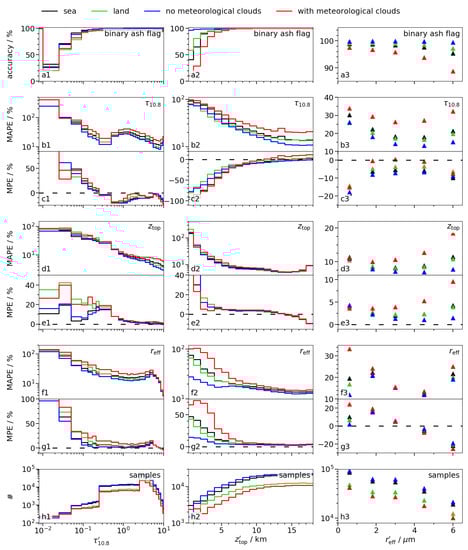
Figure 1.
Estimations of the accuracy of the binary ash flag (a), and MAPE and MPE for the retrievals of (b,c), (d,e) and (f,g) based on the simulated test data sets; the columns show the performance for different (1), (2) and (3); for (a–c) the test data set A is used, for (d–g) test data set B [2]; for (b,c) only ash-loaded samples are considered; the sample distribution of test data set B is shown in (h); different subsets are shown, i.e., only sea (black) or land (green) surfaces, only samples with meteorological clouds (red) or without meteorological clouds (blue).
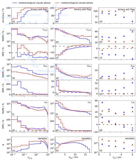
Figure 2.
Similar as in Figure 1: Estimations of the accuracy of the binary ash flag (a), and MAPE and MPE for the retrievals of (b,c), (d,e) and (f,g) based on the simulated test data sets; the columns show the performance for different (1), (2) and (3); for (a–c) the test data set A is used, for (d–g) test data set B [2]; for (b,c) only ash-loaded samples are considered; the sample distribution of test data set B is shown in (h); only samples with meteorological clouds above (blue) and below (red) the volcanic ash layer are considered.
For the binary ash flag, high accuracies of 90–100% are found for usual ash clouds () and in absence of volcanic ash (left-most bin in Figure 1a1). The additional presence of meteorological clouds decreases the accuracy: if they are above the ash layer the difference is of the order of 20%, whereas the influence is much smaller when they are below. This demonstrates that ash layers might often be hidden by the meteorological clouds above. The accuracy is also close to 100% for , but decreases with decreasing . The latter might be partly connected to the impact of water vapor above the ash cloud, as their column load above the ash layer increases with decreasing . However, as the accuracy decreases only slightly for compared to higher in the absence of meteorological clouds, the impact of water vapor appears to be limited. The presence of meteorological clouds leads to a much worse performance, especially for and if the meteorological clouds are above the ash layer, where the accuracy drops well below 50%. The dependence on is generally small, except when meteorological clouds are present above, leading to a decreasing accuracy with ~90% for , but less than 60% for . The dependence on the surface (land/sea) is small.
For the regression ANNs, the MAPE generally decreases from roughly 100% for / to less than 30% for / with increasing and , and is up to 35% with respect to . In all cases, the MAPE is smallest in the absence of meteorological clouds and largest in their presence, with significantly larger errors for meteorological clouds above with respect to and , and for meteorological clouds below with respect to . The MAPEs for land and sea surfaces are again rather similar.
On average, the retrieval of is biased towards high values for (i.e., ) and towards low values otherwise (); the MPE has values of −20 to 60% for . The MAPE has minima for around 0.3 and 8; the first minimum might be explained by the increased sample weights applied during training for at corresponding values [2]. For , the retrieved is underestimated with the MPE being −50 to −100% for and 0 to % for .
The retrieved is generally overestimated, with MPEs up to 50% but below 20% for and below 10% for . The bias is larger for optically thin ash clouds (e.g., ) with meteorological clouds above, whereas nearly no bias is apparent in the presence of meteorological clouds below. For , the retrieval error of slightly increases again; a physical reason might be that at high latitudes the tropopause is located at similar heights, such that the disappearance or inversion of the vertical temperature gradient makes the determination of more difficult.
The retrieved is overestimated for all values of and ; the MPE becomes >50% for and between 10% and more than 140% for , strongly depending on the presence of meteorological clouds. For , the retrieved is overestimated, and underestimated beyond; the MPE is generally between −20% and 20%.
Our simulated test data sets consist of samples which are calculated for specific geographical locations. The latitude/longitude coordinates are drawn randomly, but are equally distributed with respect to the SEVIRI disc [2]; thus, more samples are located around 0 N, 0 E than at larger viewing zenith angles. The georeferenced test data are used to investigate the dependence of the accuracy, POD and FAR of the binary ash flag on the geographical position in Figure 3, and the MAPE and MPE of the regression ANNs in Figure 4. In all cases, four different subsets are investigated: with meteorological clouds, without meteorological clouds, with meteorological clouds above and below (as defined before). The samples are arranged in boxes of , except for the FAR in Figure 3c1,c2, which is given for boxes to accumulate enough samples given its small numerical value. The decreasing sample density towards the edges of the plots can explain the worse retrieval performances at higher viewing zenith angles. Thus, we focus on the central regions of around 0 N, 0 E.
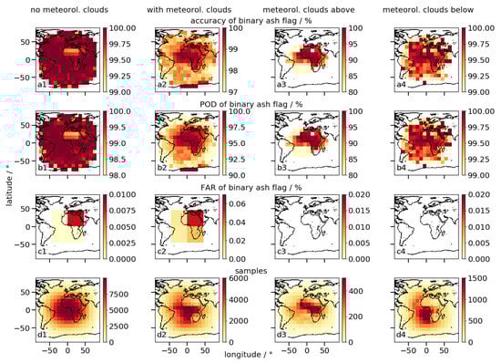
Figure 3.
Estimations of the accuracy (a), the POD (b) and the FAR (c) for the binary ash flag for different geographical coordinates and subsets without meteorological clouds (1), with meteorological clouds (2), with meteorological clouds above (3) and below (4) a volcanic ash layer; the number of samples is given in (d); no metrics are shown if a grid cell contains <100 (<50,000 for FAR) samples; mind the different color scales.
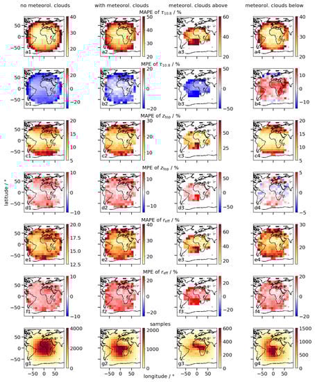
Figure 4.
As in Figure 3, but given are MAPE and MPE for the retrieval for (a,b), (c,d) and (e,f) and the number of samples (g) according to test data set B.
The binary ash flag has a high accuracy and POD (both close to 100%) in the absence of clouds except for the desert regions of Northern Africa and the Arabian peninsula, where both metrics decrease by 1–2%, whereas the FAR rises to about 0.008%. This might be connected to the surface emissivity of quartz-rich soils that can lead to a negative 10.8–12 [7]. In the presence of clouds, the accuracy and POD remain close to 100% above Africa, especially above the tropical forest and in proximity of the equator; otherwise the metrics decrease by up to 3% and 10%, respectively. The decrease is even more pronounced if meteorological clouds are above, which might be connected to the fact that the simulated samples are mostly located above tropical Africa; thus, the ANNs are in this case mainly exposed to samples of a very specific type. Meteorological clouds below are predominantly above the south east Atlantic off the coast of Africa, where an extensive marine stratus deck at low altitudes is usual [8]. The non-uniform distribution of the different sample types resembles reality, as the occurrence of meteorological clouds in the radiative transfer simulation is based on their presence in the ECMWF model [2]. To try to improve the performance of the ANNs for the physically less common cases, one could increase their amount in the training data set in the future, by specifically selecting those samples during the data set creation, or by increasing their sample weight during the training. However, this would also distort the underlying probability distributions, e.g., by artificially increasing the number of samples with meteorological clouds above the ash layer above the Atlantic, the corresponding probability would be higher for the training data set than in reality. A priori it is not clear whether this would improve the overall performance of the algorithm. Note that other retrievals exhibited similar properties as the binary ash flag, e.g., the ice cloud retrieval CiPS had the highest POD above forest for cirrus clouds with an optical thickness up to 0.5, and at the same time a high FAR above equatorial Africa as cirrus clouds often occur in this region (i.e., above tropical rainforests) and, thus, corresponding samples made up a significant part of the used training data set [9,10].
The retrieval of has a MAPE of mostly 20–30%, independently of meteorological cloud presence. Again there is a high MAPE of more than 60% above the Atlantic west of southern Africa if meteorological clouds are above the ash. is generally underestimated with MPEs of 0 to −20%, except if meteorological clouds are below the ash layer, which leads to MPEs of 0–15%.
The retrieval of shows a latitudinal dependence of the MAPE: it is 5–10% at the equator, but rises towards the poles up to 20% at ±50N. Similarly, the MPE rises from ~0% around the equator to about 10%. A reason for the latitudinal dependence of MAPE and MPE could be that the ANN might learn mainly the vertical temperature profile at the tropics, as there the sample density in the training data is the highest. Since the temperatures are generally lower towards the poles [11], the retrieved from the measured brightness temperatures using the tropical temperature profile is systematically too high. Theoretically, this issue might be overcome by using a training data set of samples equally distributed over the complete latitudinal range, again either by accordingly increasing the amount of samples or the weight of the given samples. Then there should be comparable focus on all the different temperature profiles. The ANN’s decision on which temperature profile to use could be based on the latitude, but also on, for instance, the time of day and day of year, all of which are used as input data for VACOS. However, another problem might be the decreasing height of the tropopause and the corresponding vertical temperature inversion at higher latitudes, which makes it harder to deduce from the measured brightness temperatures for ash clouds above the tropopause. Differences in the surface emissivity due to ice and snow surfaces [5] might also introduce errors in the most poleward regions. The last two issues would not be solved by using a training data set evenly distributed across latitudes.
The retrieval of is generally overestimated, with MAPEs at the equator around 15% if no meteorological clouds are present, and 20% on average in their presence. Again, the error is higher above the Sahara in the absence of meteorological clouds.
2.3. Detection of Volcanic Ash
Volcanic ash can be detected using the following threshold rules: a sample is classified as ash-containing if one of 12–10.8, or the probability for ash due to the binary ash flag is larger than a given threshold 12–10.8,thrs, or , respectively. Notice that the first possibility is independent of VACOS. Figure 5 shows POD and FAR for all three methods for different thresholds. Generally, by increasing the threshold the POD as well as the FAR decrease. Thus, it is necessary to find a trade-off between both properties. In case of doubt a higher POD is favored with regard to the relevance of ash detection in aviation-security. As thin ash layers are harder to detect (Section 2), two subsets are considered besides the full test data set: samples with and . Using 12–10.8 (e.g., [7,12,13]) with 12–10.8,thrs = gives a POD of 100% and a FAR of about 10%. The former is due to the selection of ash samples in the simulated data sets, i.e., only ash-loaded samples with 10.8–12 have been considered [2]. For 12–10.8,thrs = 1.58, the POD is ca. 70% and the FAR is about 0.25% for the full test data set. For the subsets of lower , the POD is much lower, whereas the FAR remains high. Using leads to higher PODs compared to 12–10.8,thrs for all three sets of test data, the curves move towards the upper left corner of Figure 5. Again the PODs are smaller for lower . For example, leads to a FAR of 1% and a POD of 98.7% (95.4%, 86.8%) for the full test data set (only < 0.5, <0.2). Using leads to an even better performance in all subsets: up to roughly , the POD decreases only slightly, whereas the FAR decreases by multiple orders of magnitude. Only for higher , the POD drops as well. For , the FAR is 0.008% and the POD is 98.6% (95.5%, 88.2%) for the full test data set (only < 0.5, <0.2).
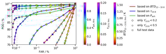
Figure 5.
Estimations of the POD and the FAR for the detection of volcanic ash using 12–10.8 (connected by a red line), (blue line) and the probability of the binary ash flag for ash (green line), and a corresponding threshold (color of marker, see colorbars); different subsets of the test data set [2] are used and encoded in the marker type, i.e., the full data set (square), only samples with (circle) and <0.2 (diamond); the x-axis is linear left of the black, dotted, vertical line and logarithmic right of it.
Instead of subsets defined by the as in Figure 5, one can also select sets according to : For , corresponding to 0.2 g m−2 when considering a mean mass extinction coefficient at of 200 m kg−1 [2], and , a typical regime for distal volcanic ash clouds (Section 4), the POD is ca. 93% and the MAPE for roughly 40%, whereas leads to a POD of 99% and a MAPE of 26%. For the ash-free samples, the FAR is about 1%.
3. Sensitivity to Volcanic Ash Cloud Profiles
For the training data set, we made the ad hoc assumption of a single, homogeneous volcanic ash layer with up to 18 km, geometrical thicknesses up to 7.2 km and up to 30 [2]. Here we consider the sensitivity of the brightness temperatures and the ANNs on the ash cloud profile. In all cases we apply the refractive index of Eyjafjallajökull ash [14], a log-normal particle size distribution with , a geometric standard deviation and a representative shape distribution of spheroids as considered in Piontek et al. [3]. A thick ash cloud is assumed with , corresponding to for a mass extinction coefficient at of 200 /. This order of magnitude of can be found in close proximity of a volcano (Section 5); for lower , the absolute impact of the investigated macrophysical properties on the brightness temperatures is assumed to be smaller.
Using ECMWF ERA5 data for 2010 and the methods described in Piontek et al. [2], a random set of 500 atmospheric and geographical conditions is chosen and used for the calculation of the brightness temperatures for each cloud setting. Only cases without meteorological but with volcanic ash clouds are investigated as meteorological clouds were already shown to influence the retrievals significantly.
3.1. Multiple Ash Layers
To quantify the variability in the brightness temperatures due to multiple layers, we compare a single layer with four different multi-layer structures, Figure 6a. All four setups keep and fixed (i.e., the parameters that are retrieved by the ANNs). Layers #1 and #2 also keep the mass concentration c fixed and introduce a gap in the volcanic ash cloud. Layers #3 and #4 keep the cloud bottom height fixed but increase c. The brightness temperatures of the infrared channels of SEVIRI are simulated and the differences compared to the single layer are calculated, Figure 6b. Layers #1 and #2 show that the brightness temperature increases with a decreasing height for the lower ash layer; the differences are generally positive, as more of the mass is in warmer parts of the atmosphere. For a gap of the differences can be > , but for a gap of 2 the differences are even > 2 , with outliers even > 3 . For the more condensed structures #3 and #4, the differences are mostly between 0 and and negative as more of the mass is in cooler parts of the atmosphere. Figure 6c shows the relative differences in the retrievals with respect to the true values. The median retrieval is overestimated by ca. 3%, the retrieved is underestimated by about 7%. In both cases is the influence of multi-layer structures compared to single layers on the order of 1%. The median retrieved for a single layer is about 20% higher than the true value. Again structure #2 leads to the largest difference: here the median retrieved is about 10% lower than the true value. The structures #3 and #4 lead only to minor differences compared to the single layer.
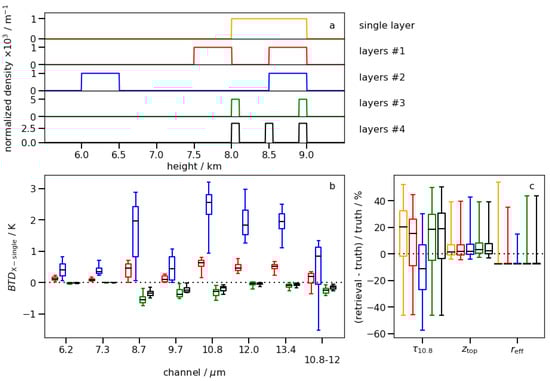
Figure 6.
Analysis of the impact of different ash layerings with (a) the normalized vertical cloud profiles for multiple layers, (b) the of different channels between a single mass layer and the layerings in (a), (c) the relative differences in the retrievals of , and compared to the true values for the different layerings in (a); for each setup 500 simulations are averaged (see text); the boxplot shows the median, first and third quartile (box) and the 5th and 95th percentile (whiskers).
3.2. Non-Homogeneous Ash Profiles
The assumption of a uniform ash layer [2] is often not fulfilled in reality, where vertical ash mass profiles do not have discontinuities and might have a clear peak [15,16,17]; thus, a more realistic description would be a normal distribution or the -sigmoid distribution (Appendix B and [18]), which has the ability to approximate uniform and normal distributions as limiting cases, Figure 7a. To quantify the influence of the cloud profile, different assumptions are compared. A uniform cloud with a typical height of 8–9 km is assumed [2]; thus, the mean height is and the standard deviation . These values are assumed for the other distributions as well. For the -sigmoid distribution, the variables parameterizing the lower and upper end of the cloud are varied (-sigmoid #1: and , #2: and , #3: and ). The continuous distributions are cut off at and ; within this regime they are modeled by 100 sublayers of depth , each having a mass volume concentration corresponding to times the density of the normalized vertical mass distribution at the mean height of the sublayer. The brightness temperatures of the infrared channels of SEVIRI are simulated and the differences of the various profiles compared to the uniform distribution are calculated, Figure 7b. The absolute differences are mostly < and, therefore, smaller or of the same order as the instrumental noise [19]. Outliers are < . In some channels (e.g., or ) the differences for all profiles are mostly negative, indicating that a more realistic cloud profile might lead to slightly lower brightness temperatures. Applying the ANNs to the different profiles leads to negligible differences (not shown).
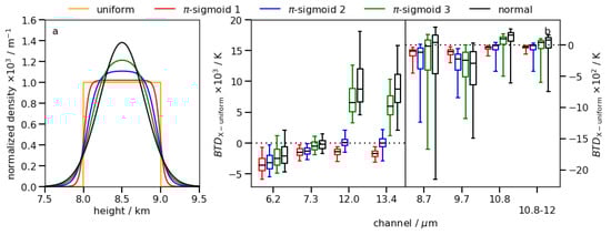
Figure 7.
Analysis of the impact of different ash profiles with the same mean and standard deviation with respect to the height of the center of the cloud, with (a) the different profiles and (b) the of different channels between a uniform vertical mass distribution and the other distributions in (a); for each setup 500 simulations are averaged (see text); the boxplot shows the median, first and third quartile (box) and the 5th and 95th percentile (whiskers).
3.3. Geometrical Ash Cloud Thickness
Although the geometrical cloud thickness is varied within the training data set, it is not retrieved explicitly by the ANNs, and it is not clear whether they are able to derive this information internally as a side product. Here we quantify the impact of this property with respect to the brightness temperature and the retrieval results. Therefore, layers with thicknesses of 0.5 km, 1 km, 2 km and 3 km are considered, with and kept constant. The difference compared to the 1 thick case are considered, Figure 8a. As expected, thicker clouds have higher brightness temperatures as more mass is in lower and warmer parts of the troposphere; the thinner layer leads to lower brightness temperatures. The geometrical cloud thickness introduces a variability of the brightness temperatures of −1 to −4 . Figure 8b shows the results of the retrievals. Whereas the impact of the cloud thickness is generally negligible for , an increased thickness (and, therefore, decreased cloud base height) leads to smaller retrievals for and . The influence on the latter is only small (between −4% and 8%), but the former can exhibit differences of more than 20% comparing cloud geometrical thicknesses of 0.5 and 3 .
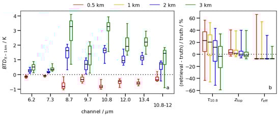
Figure 8.
Analysis of the impact of different geometrical ash layer thicknesses, with (a) the of different channels between a layer with a thickness of 1 and the other thicknesses, (b) the relative differences in the retrievals of , and compared to the true values for the different layer thicknesses; for each setup 500 simulations are averaged (see text); the boxplot shows the median, first and third quartile (box) and the 5th and 95th percentile (whiskers).
Comparing different volcanic ash clouds, geometrical layer thickness and multi-layering represent the largest sources of error. The uncertainties introduced by those properties with respect to the brightness temperatures are larger than the instrumental noise [19] and are of the order of 30% for , 5% for and negligible for . The shape of a single layer profile is negligible.
4. Comparisons with Independent Measurements
To prove the applicability of the retrievals to real data, we compare our results with other in situ and remote sensing measurements as well as the outcome of the predecessor VADUGS for selected scenes.
4.1. Puyehue-Cordón Caulle Eruption (2011)
Lidar measurements represent an excellent source for comparison since they provide accurate estimates for and the vertical profile. Here we use data from the CALIPSO/CALIOP [20] version 4.10 level 2 aerosol products, which include information about volcanic ash layers in the stratosphere [21]. The extinction profiles of those layers were used to calculate their optical depth at 532 , which was converted to using a mass extinction coefficient of 690 m2 kg−1 [22,23]. corresponds to the top of the uppermost ash layer. Only ash samples with extinction quality control flag zero (initial lidar ratio resulted in stable extinction retrievals, i.e., “unconstrained” retrievals) or one (when the lidar ratio could be inferred directly from the data, i.e., “constrained” retrievals) were used. For the unconstrained retrievals, a lidar ratio of 58 (median of the directly retrieved lidar ratios) was used to update the ash optical depth to correct for the low bias resulting from the use of the default lidar ratio of 44 for ash in CALIPSO version 4.10. The final data set has a horizontal resolution of 5 and a vertical resolution of 60 .
The six scenes in consideration are listed in Table 3 and sketched in Figure 9; data are plotted in Figure 10 (blue line). They show volcanic ash clouds from the Puyehue-Cordón-Caulle eruption, starting at 4 June 2011. The flyovers took place above the southern Atlantic ocean between 15 June 2011 and 18 June 2011 during day and night. was 10–15 and reached up to ; note that the uncertainty of the latter is roughly a factor of 2, see Figure 10. is not derived from CALIOP data, but Bignami et al. [24] used MODIS data to retrieve mean values of 4– 6 within 300 from the volcano. Due to sedimentation processes should be smaller in the scenes considered here. Ishimoto et al. [25] retrieved from IASI spectra at distances of ~ 1000 for most samples . The silica content was around 70 or slightly below [14,26,27].
Table 3.
Investigated CALIPSO flyovers in June 2011 with timespan, coordinates of start and endpoint, number of samples and track number according to Figure 9.

Figure 9.
Overview of the CALIPSO transits (green) as described and numbered in Table 3 with the corresponding VACOS retrievals of (red colors) and the cirrus flag of CiPS (blue); Figure (a,b) are made up of three stripes each, showing the VACOS and CiPS retrievals at the times of the corresponding CALIPSO transits; thus, the retrievals of the three stripes in each plot correspond to three different times.
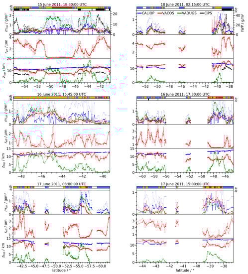
Figure 10.
Pixel classification (ash) and retrievals of (derived from ), and as determined using CALIOP (blue), VADUGS (green) and VACOS (red) for volcanic ash clouds of the Puyehue-Cordón Caulle eruption 2011 above the Atlantic on 15–18 June 2011, see Table 3; the times above the plots indicate the start of measurement of the SEVIRI image used; the VACOS regression results are averaged on pixels with the pixel result shown in faint red, whereas the for the classification the single pixel result is shown; the upper uncertainty of by CALIOP is indicated in faint blue; the ash classification shows: clear skies (green), meteorological clouds (blue), volcanic ash (red), ash and meteorological clouds (orange); a cirrus cloud flag (ice) and, if applicable, the ice water path (IWP) are derived using CiPS (black); the cirrus flag shows: cirrus (black), no cirrus (white); the latitude refers to the position of CALIPSO; note that vertical axes are scaled differently in the plots.
We compare the CALIOP measurements with the results of the ANNs applied to SEVIRI images at close times. The coordinates given by CALIPSO are corrected such that the light path of the SEVIRI measurements penetrates the top of the ash cloud (parallax correction). The regression retrievals are shown on a single pixel basis (faint red), and after a mean filter of pixels was applied (red); the classification result is shown only on a single pixel basis. is converted to using a mean mass extinction coefficient at of 152 m2 kg−1, which holds for silica contents of 70 and [2]. Additionally, the retrievals of volcanic ash by VADUGS and of cirrus clouds by CiPS [9,10] are shown in Figure 10. The MAPE and MPE for the retrievals of and are given in Table 4, the PODs using and and different thresholds are given in Figure 11.
Table 4.
Comparison of the retrievals VADUGS and VACOS against CALIOP data; different subsets depending on from CALIOP are considered; the MAPE and MPE for the retrieval of and are calculated; the retrieval is analyzed after application of a 3 × 3 pixels (px) and 5 × 5 px uniform filter.
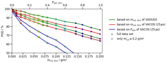
Figure 11.
Estimations of the POD of volcanic ash using and of VACOS (connected by red and blue lines, respectively) and of VADUGS (green line), and a corresponding threshold; different subsets of the test data (Table 3), are used and encoded in the marker type, i.e., the full data set (square), only samples with target (circle).
Again the mass load due to CALIOP (i.e., the “true” value) is denoted . For , the retrieval of using VADUGS has a MAPE of 62% and a MPE of 12%, indicating a slight overestimation; this is visible in Figure 10 for 15 June 2011 at 18:30 UTC or 16 June 2011 at 17:30 UTC, although the VADUGS results are mostly within the uncertainty interval of the CALIOP data. VACOS has a smaller MAPE of 56%, but underestimates due to a MPE of %. Remember that VACOS is more complex than VADUGS, consisting of four instead of only one ANN, using more input features, with each ANN having three compared to just a single hidden layer (although with 100 instead of 600 neurons per hidden layer) [1,2]. As a consequence, VACOS has significantly more trainable parameters and has the potential to learn more complex functions, such that their pixelwise application can lead to rather abrupt jumps in the retrievals; this can be seen, for instance, at 18 June 2011, 02:15 UTC in Figure 10 and the corresponding track 6 in Figure 9b. Thus, the VACOS retrievals are also calculated after the application of a and a pixels uniform averaging, which leads to a further reduction of MAPE (47% and 45%, respectively) and MPE (% each). Note that this MAPE is similar to the values found for the simulated test data. Whereas the reduction in the errors is of the order of 10% when comparing the unfiltered results with the results after an averaging over pixels, the further decrease is only on the order of a few percent when considering pixels. Note that averaging over even larger areas might worsen the retrieval of fine structured ash clouds, e.g., thin plumes close to the volcanic vent; therefore, this is not done here. Considering the full CALIOP data set leads to significantly higher errors than for the subset with , showing that the retrieval of thin ash layers is much harder. VADUGS has a MAPE of 123% and a MPE of 70%. VACOS has higher errors before averaging the results, but performs better after averaging over pixels, with a MAPE of 111% and a MPE of 43%. Averaging over pixels slightly increases the errors. The reason might be that small are often located at the edges of ash clouds, where the averaging over larger areas includes ash-free pixels. The retrieval of is mostly independent of the subset and the averaging for both VADUGS and VACOS. MAPE and absolute MPE of VADUGS are 70–75%. Although VADUGS is able to retrieve the correct heights in some cases (especially when ), it often strongly underestimates ; compare, for instance, 16 June 2011 at 15:45 UTC in Figure 10. VACOS retrieves with a MAPE , but also slightly underestimates the true height as indicated by a MPE of %. The retrieved exhibits large variations with values between (the lower end of the training data regime [2]) and 4 ; thus, they are smaller than the values retrieved by Bignami et al. [24] close to the volcano, but significantly larger than the results by Ishimoto et al. [25]. Note that the lowest are retrieved for the highest (e.g., at 16 June 2011, 17:30 UTC). As the errors of decrease with increasing (as shown in Section 2), the retrieved is most reliable for thick clouds. The small also supports the choice of the mass extinction coefficient at above.
The classification ANN indicates the presence of volcanic ash especially for thick ash layers, whereas thinner layers are often misclassified as meteorological clouds. The POD using of the resulting binary ash flag and using of VADUGS and VACOS (compare Section 2.3) are given for different thresholds in Figure 11. For VACOS, the averages over pixels are used for and the single pixel result for . VACOS performs slightly worse than VADUGS with respect to volcanic ash detection using . Setting leads to a POD of 65–75% for VACOS; for , the POD is around 80%. Both values are significantly smaller than for the simulated test data set, which indicates that there are differences between the simulated data set and data collected in reality. However, note that the different performances of VADUGS and VACOS can be explained in part by the retrievals MPEs: VADUGS overestimates whereas VACOS underestimates it. Correcting this would lead to a decrease of the POD of VADUGS and to an increase for VACOS. Furthermore, the assumed mass extinction coefficient at for the transformation of to has an impact for VACOS: using a smaller value increases due to VACOS and consequently also the POD. The performance of the binary ash flag is significantly lower here as compared to the simulated test data and the results using the retrieved , independently of the threshold; leads to a POD around 60%. This indicates that the use of for detection is more reliable than the classification ANN in this situation. The FAR has not been quantified here, but Figure 9 shows mostly large-scale structures representing the ash clouds, and only in some scenes are tiny patches with significant which are not connected to the ash clouds and might be false detections. Thus, we assume the FAR to be reasonably low.
Two scenes, 15 June 2011 at 18:30 UTC and 18 June 2011 at 02:15 UTC, contained cirrus clouds underneath the ash layer, with ice water paths up to 20 and 40 , respectively. In both cases the cirrus has a moderate impact on the retrieved , but the retrieved is significantly increased in the presence of the cirrus clouds; meanwhile, the retrieved drops to zero, especially at 18 June 2011, 02:15 UTC. This shows that it seems recommendable to always evaluate VACOS results alongside cirrus retrievals.
4.2. Eyjafjallajökull Ash Cloud (17 May 2010)
Following the 2010 eruption of the Eyjafjallajökull, the Deutsches Zentrum für Luft- und Raumfahrt (DLR, the German aerospace center) and the Facility for Airborne Atmospheric Measurements, United Kingdom (FAAM) independently performed airborne in situ and lidar measurements of the volcanic ash clouds [15,16,28]. Here we consider measurements from 17 May 2010, when both aircraft simultaneously investigated the same ash cloud above the North Sea [17]. The VACOS retrieval of and the cirrus mask of CiPS are given for an example scene, Figure 12b, showing that the ash and ice clouds are well separated. VACOS can be compared to volcanic ash detections by Schumann et al. [15] for a scene two hours later, using 10.8–12 with a threshold of for detection and applying a low-pass filter (Figure 15 in [15]). Both methods exhibit similar distributions of the optically thickest ash clouds, e.g., patches above the North Sea, west of Norway and above Iceland. However, VACOS finds additional, extended ash clouds with above Germany and Norway. The ash cloud investigated by DLR and FAAM as well as the flight trajectories of the two aircraft are sketched in Figure 12a.
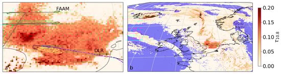
Figure 12.
VACOS retrieval of at 17 May 2010, 16:00 UTC; shown is (a) the North Sea between the Netherlands and England, and (b) north-western Europe up to Iceland; blue areas are covered by cirrus clouds according to CiPS [9]; panel (a) also shows the flight tracks of the DLR Falcon aircraft (with different parts of the track in black, yellow, blue and violet) and the FAAM aircraft (green) [15,16].
Schumann et al. [15] provided in situ measurements with a time resolution of 1 for the altitude and 10 for the mass volume concentration. To derive the latter they made two different assumptions on the refractive index of the volcanic ash (case L: i, case M: i; at 630 ), leading to an upper and a lower estimate of the mass concentration. A third case (H: i) was evaluated by Schumann et al. [15], but based on their full analysis they expected the true value to be between case L and M. Ball et al. [29] measured for the refractive index of Eyjafjallajökull ash at a wavelength of 650 a real part of and an imaginary part of , which would support case L. Schumann et al. [15] pointed out that the imaginary part of the refractive index was the major source of uncertainty. The effective radius was estimated to be 0.65– [15]. Considering altitude and mass concentration shows that the aircraft enters the ash cloud from above at 15:50 UTC, reaches a minimum altitude around 16:35 UTC (yellow in Figure 12), and rises afterwards until it leaves the ash cloud again at ca. 17:00 UTC (blue in Figure 12), see Figure 13. Data of the two transits (from above and from below) are treated separately; the corresponding measured vertical mass profiles as well as their linearly interpolated and over 200 averaged profiles are shown in Figure 14. Although different parts of the ash cloud are probed during the two flight legs, the vertical mass profiles are relatively similar, indicating a horizontally homogeneous ash distribution (over distances in the order of ~ 50 ). However, vertically the ash cloud has a highly variable mass profile. Ash cloud top and bottom height are roughly at and , respectively. Integrating the vertical mass profiles of Figure 14 and averaging of the two flight legs gives and for the lower (L) and upper (M) estimate, respectively. The DLR data are shown in the left panel of Figure 13.
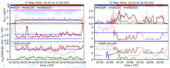
Figure 13.
Pixel classification (ash) and retrievals of (derived from ), and as measured in situ by DLR (blue, left panel [15]), derived using an airborne lidar by FAAM (blue, right panel [16]), VADUGS (green) and VACOS (red) for an Eyjafjallajökull ash cloud above the North Sea at 17 May 2010; the VACOS regression results are averaged on pixels with the pixel result plotted in faint red, whereas only the single pixel result is shown for the classification; also VACOS retrievals of and for are plotted in faint red; for the in situ data, only mean values or upper and lower estimates are given; for the lidar-derived data, the upper and lower uncertainty of is indicated in faint blue; the ash classification shows: clear skies (green), meteorological clouds (blue), volcanic ash (red), ash and meteorological clouds (orange); the altitudes of the aircrafts are given (grey dashed).
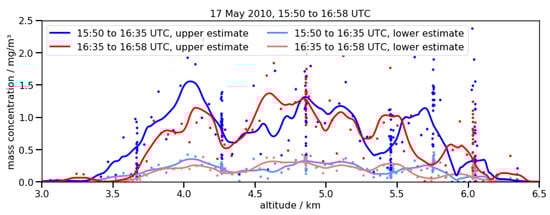
Figure 14.
Vertical mass profiles of the volcanic ash cloud as measured by Schumann et al. [15] during two flight legs (see text) indicated by the color (blue, red); based on different assumptions, there is an upper estimate (M, bold colors) and a lower estimate (L, faint colors) of the in situ measurements; 10 averages are given as dots, derived 200 means are shown as lines.
From Marenco et al. [16] the lidar-derived mass profiles are used, which have a vertical resolution of 45 and a temporal resolution of 60 , corresponding to a horizontal resolution of at typical aircraft speeds. The uncertainty of the masses is given by a factor of two [16]. We calculate by integrating the vertical mass profile, whereas we define as the height where the mass volume concentration (median over 315 , i.e., 7 height levels) exceeds 50 ; averaging kernel and mass concentration threshold are based on visual inspection of the mass profiles. In situ measurements performed in April and May 2010 by the FAAM led to of ca. 0.5–2 [28]. The FAAM data for the flight at 17 May 2010 are shown in the right panel in Figure 13. Just as the DLR, the FAAM aircraft dipped into the ash cloud several times; to avoid incomplete mass profiles, measurements of and are discarded if the FAAM aircraft is <500 above or if the aircraft is below 5 .
Apart from different instrumentation and processing for the in situ measurements [17], the flights by DLR and FAAM followed fundamentally different strategies: the DLR aircraft remained in an self-contained area well within the ash cloud, hence the relatively constant , whereas the FAAM entered and left the ash-containing area multiple times, see Figure 12a. Still, the data from both measurements shows some similarities, Figure 13. The lower estimate of from DLR is generally in good agreement with the maximum best estimate due to the FAAM, whereas the upper estimate from DLR and the maximum of the uncertainty of by the FAAM are both around 2 . The lower estimate of is similar for DLR and FAAM, but the upper estimate differs by roughly 1 ; differences in the ash particle size distributions were also reported by Turnbull et al. [17]. from DLR agrees with the largest estimate derived from FAAM data, but the latter varies between roughly 4 and 7 , again indicating that a more diverse area of the ash cloud was sampled.
For the VACOS and VADUGS retrievals, a parallax correction is implemented, i.e., coordinates are considered such that the light path crosses the coordinates of the DLR and FAAM aircraft at a height of 6 km and 5 km, respectively, and penetrate the observed ash clouds. The heights correspond roughly to the measured of DLR/FAAM. The SEVIRI images with a time resolution of 15 are processed and the temporally closest image is chosen for each measurement; the SEVIRI line acquisition time is considered. The FAAM’s mean aircraft velocity of ~ 146 (on ground) and a SEVIRI pixel size of roughly times (at 54 N, E) indicate that it takes the aircraft generally about 47 to cross a pixel in north–south direction and 22 in east–west direction. As the FAAM data has a time resolution of 60 , a minimum averaging of SEVIRI pixels is necessary to compare the satellite retrievals to the FAAM data, assuming the aircraft moves only in east–west direction. Based on the results of Section 4.1, an averaging over pixels is considered here. As due to DLR and FAAM data is around 1 , a mass extinction coefficient at of 200 m2 kg−1 is assumed [2]; note that this conversion factor is applied in the rest of this work when dealing with Eyjafjallajökull ash clouds. VACOS retrievals of and are shown in faint red if , as the former are ill-defined in the absence of ash clouds. The resulting retrieval data is given in Figure 13.
Considering the DLR case (left panel in Figure 13) we find that the VACOS lies at the lower end of the uncertainty interval of the DLR measurement with relatively low variability. varies between 5.5 km and 8.5 km, which includes the value found from the DLR data. For the most parts, lies well between the estimates by Schumann et al. [15]. The classification ANN flags the whole ash cloud correctly.
The FAAM measurements (right panel in Figure 13) and the VACOS retrievals for , and are generally in agreement. VACOS slightly underestimates the mass load with compared to the FAAM value of ~ before 14:00 UTC (and consequently derives too high estimates for and ), but retrieves similar around as the FAAM later on. VACOS retrieved and show plateaus around and 5 , respectively, at 14:30 to 14:45 UTC as well as 15:45 to 16:30 UTC. At other times, e.g., around 14:20 or 15:20 UTC, there are coincident increases of and , which can be attributed at least partially to thin ash clouds with at the edges of the ash clouds; thus, these retrievals can be assumed to be unphysical. Other peaks in and , e.g., around 15:00 UTC, appear although there is a significant amount of volcanic ash (i.e., VACOS retrieves ). The classification correctly classifies the major parts of the ash encounters.
Although the comparisons of VADUGS retrievals with the CALIOP results in the case of the Puyehue-Cordón Caulle ash cloud showed a good agreement, VADUGS seems hardly applicable in the present case: and are strongly underestimated in both comparisons and at all times.
4.3. Eyjafjallajökull Ash Plume at Vent (11 May 2010)
The concentrations that have been compared up to now are rather low. Here the retrieval ability closer to the vent is investigated. Researchers from the University of Iceland used a piston-driven aircraft to probe the outer parts of the ash plume of Eyjafjallajökull in 2010 at distances of 45–60 from the vent [30]. Plume heights of 3–4.3 km have been reported [30,31], and at 11 May 2010, mass volume concentrations of 0.5–2 mg m−3 [30]. Assuming a geometrical thickness of 1–2 , this corresponds to being 0.5–4 for the fringes of the ash plume; in the center of the plume the values should obviously be higher. Note that Weber et al. [30] reported the boundary of the ash plume to be inhomogeneous, with ash cloud puffs of diameter 0.5–2 . These small scale structures are not resolvable by SEVIRI [2].
As an example we consider a scene at 11 May 2010, 14:00 UTC, Figure 15. The Eyjafjallajökull ash plume moves southwards from the vent and is surrounded by different cloud fields (a). The cirrus cloud retrieval CiPS [9,10] shows ice water clouds collocated with the ash plume up to some hundred kilometers from the vent. With roughly 1–6 , the ice water path (b) is rather low (e.g., compared to the retrievals in Figure 10), and the cirrus clouds are located at 9–11 height (c), i.e., above the heights given by Weber et al. [30]. Weber et al. [30] also report that the top of the ash plume above the sea appeared white, whereas it was darker below, and significant ice contents have been found in volcanic ash plumes before [32,33,34]. The additional ice content might spoil the volcanic ash retrieval in this scene (compare Section 4.1). Note that although it was shown that aerosol layers below cirrus clouds have only a small impact on CiPS [10], the volcanic ash plume in this scene is by no means negligible (f). Therefore, the CiPS retrievals have to be treated with caution as well. The ash plume is detected by VADUGS (d), but with it underestimates the mass load by one to two orders of magnitude compared to Weber et al. [30]. The classification due to VACOS (e) shows the (mostly pure) ash plume moves southwards and then bends eastwards. A visual comparison of the classification results with (a) indicates that too few pixels might be classified as clear sky (green). The VACOS retrievals of (f), (g) and (h) are shown for pixels with . (f) shows the plume with decreasing values downwind. The upper end and the center of the ash plume show values around 3 and larger, the edges values of the order 1 ; this is in agreement with the in situ measurements by Weber et al. [30]. Downwind the plume bends eastwards. The ash has dispersed and is ca. 0.5–1 . The retrieved (g) has values of 10–12 close to the vent, which is much larger than the literature values. When the plume bends eastward, retrievals drop to 5–6 . Similarly, we find large (h) around 3 close to the volcano and then a sudden drop to values around 1 . In all three cases the sudden change in the retrievals happens at the edge of the retrieved cirrus cloud, compare (b) and (f), indicating that the presence of the cirrus cloud might lead to the overestimation of , and . Apart from the impact by the cirrus cloud, the retrievals also have some inherent limitations that might lead to inaccuracies close to the vent: the ash properties used in the training data correspond rather to those of aged ash clouds than to fresh ash (e.g., only small particles without porosity are considered) and typical gas emissions (e.g., water vapor, sulfur dioxide) have not been included [2].

Figure 15.
Retrieval results for the Eyjafjallajökull eruption at 11 May 2010, 14:00 UTC with Iceland outlined in the top of the plots; (a) false color overview composite from SEVIRI data, from CiPS (b) cirrus ice water path and (c) cloud top height, (d) from VADUGS, and from VACOS (e) the classification (color code as in Figure 10), (f) , (g) and (h) .
5. Comparison with a Model Ensemble
To check the general performance of VACOS on large scales, the retrievals are compared with the results of a volcanic ash transport and dispersion model. Note that the model is an approximation of the reality as, for instance, inaccuracies in the volcanic ash source term or the meteorological conditions are transferred to the ash distribution. Thus, the scope of this section is to quantify the agreement of the spatial distribution of volcanic ash clouds and to compare the order of magnitude of .
Here the multi model multi source term ensemble by Plu et al. [35] is used. They simulated the Eyjafjallajökull eruption at 13–19 May 2010 and the area from Iceland in the north-west to Italy in the south-east. We consider scenes every six hours. Four models were used: the atmospheric Lagrangian transport model FLEXPART, the Eulerian chemical transport model MATCH and the chemical transport models MOCAGE and WRF-Chem, considering in varying ways phenomena such as atmospheric transport and mixing, gravitational settling, wet and dry deposition, and chemical reactions. An a posteriori source term is used, determined using a FLEXPART-based optimal estimation model and estimates of from satellite data, as well as upper and lower bounds for the source term based on the uncertainties of the optimal estimation result. All models spin-up for at least 3 days, their results are vertically integrated and averaged on a grid, as only the large-scale distribution of ash is of interest here. The ensemble result is the median of all simulations.
VACOS and VADUGS retrievals of are averaged on the same grid. Instead of the simple uniform averaging of the retrieval results performed in Section 4, the following accumulation rule is applied to alleviate the impact of (a) the different spatial resolutions, (b) possible temporal and spatial shifts between model and satellite retrieval and (c) false satellite detections: a grid cell at time t is assumed to be ash-contaminated if at least a fraction of all pixels within the cell and within the time exceeds a threshold of ; then the estimate of is the mean of this fraction of the pixels. For VADUGS, and is used. For VACOS, three different settings are applied: the same as for VADUGS; and ; and . Grid cells covered by cirrus clouds according to the retrieval COCS [36] are discarded.
Three example scenes are shown in Figure 16. The model ensemble shows thick volcanic ash plumes close to the Eyjafjallajökull with , and ash clouds with extending over large parts of Europe. VADUGS detects only very limited ash clouds, which correspond spatially to the thickest parts of the simulated ash clouds but with a lower . However, in some cases it does not detect ash directly at the volcano, although a prominent plume is simulated. VACOS detects more ash contamination, especially also the plumes in the direct surroundings of the vent, and retrieves higher for them compared to VADUGS. Still, the model ensemble often produces larger ash-loaded areas in the surroundings of the volcano than retrieved by VACOS. At greater distances VADUGS hardly retrieves any ash, whereas VACOS regularly finds ash clouds above central Europe. For instance, in Figure 16b3 volcanic ash is found above the Atlantic north of Scotland, south-east England and at the Atlantic coast of France; then, the ash cloud bends towards north-east and continues over central France and central Germany with concentrations around 0.2–0.3 . The model ensemble produces a similar distribution, but the ash cloud heads further south after the bending, continuing above the Mediterranean sea (panel a3). Similar offsets between the model and the VACOS retrieval are also visible comparing the other two scenes; in both cases there are faint ash clouds that are detected further east by VACOS than they are simulated by the model ensemble. This indicates that the model is less reliable at large distances, e.g., above central Europe, which might also influence the following comparisons, but at the same time it confirms that the satellite retrievals over here are plausible and reliable.
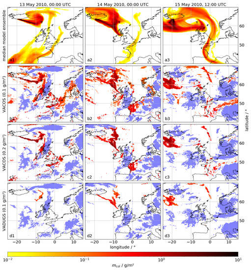
Figure 16.
(red) according to the median of a model ensemble (a), VACOS ( and , ; b and c) and VADUGS (, ; d) for three scenes (1: 13 May 2010, 00:00 UTC; 2: 14 May 2010, 00:00 UTC; 3: 15 May 2010, 12:00 UTC); for the model is not shown; cirrus presence according to COCS is indicated (blue).
Figure 17 shows the POD and the FAR for the different retrievals and accumulation rules with respect to different subsets of the model ensemble. Furthermore, offsets up to 100 are taken into account, i.e., an ash-loaded grid cell of the simulation is considered detected if the retrievals find ash within the given radius, and a retrieved ash-loaded cell is considered a false alarm if no ash is modeled within the same radius. VADUGS is found to have the smallest POD and FAR, whereas both metrics are larger for VACOS but decrease for more conservative accumulation and threshold rules. Increasing the offset distance leads to significant increases in POD, whereas the decrease of FAR is mostly rather small. When increasing , the POD as well as the FAR increase. The latter is explained by samples with but , existing either because of overestimation by the retrievals, or in the case of the subset with due to , such that samples with correctly retrieved mass loads in between those two values lead to false alarms. Considering and an offset of 100 leads for VADUGS to a POD of ~30% and a FAR of 0.02%, whereas VACOS (with , ) has a POD of close to 60% at a FAR of about 2%. The PODs increase by ~20% for and by 25–30% for . In the latter case, the POD of VACOS is nearly 90% and the FAR is 2–3%.
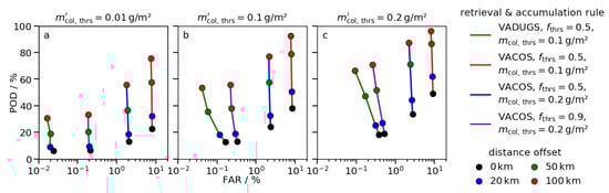
Figure 17.
Estimations of the POD and the FAR for the detection of volcanic ash using of VACOS (connected by red, blue and violet lines) and of VADUGS (green line) applying different thresholds and accumulation rules (see text); different thresholds for the model data are used, e.g., only samples with (a), ≥0.1 g m−2 (b) or ≥0.2g m−2 (c) are classified as ash-containing; only pixels in absence of cirrus clouds are used, ca. 66,000 in total; different offset distances between the model and the satellite data are considered and indicated by the marker color (see text).
Table 5 gives the MAPE and MPE for the retrieval of for VADUGS and VACOS, different accumulation and threshold rules and different subsets of the modeled data, not considering any distance offsets. For the MAPE is around 100% and the MPE is % for VADUGS, whereas for VACOS the MAPE is higher (106–138%) and the MPE is less negative ( to %), i.e., the underestimation is smaller compared to VADUGS. However, considering only grid cells that are classified as ash-contaminated by the model and the retrieval, i.e., and , the MAPE and MPE of VADUGS change to 65% and %, respectively. Using the same accumulation and threshold (, ) for VACOS leads to a MAPE of only 57% and a MPE of 0%; thus, the retrievals of VACOS are in better agreement with the model results than those of VADUGS, indicating that VACOS is more reliable for these mass concentrations.
Table 5.
Comparison of the retrieval of VADUGS and VACOS against the model ensemble median; MAPE and MPE of different subsets depending on from the model ensemble and from the satellite retrieval are considered; for VACOS a mass extinction coefficient at of 200 m2 kg−1 is considered for the conversion of to ; different accumulation rules and thresholds are used for the satellite retrievals; pixels with cirrus cloud presence are excluded.
6. Unraveling the Black Box: How Do the ANNs Work?
In this section, we aim to shed light upon the working principles of our ANNs. Therefore, we first perform additional radiative transfer calculations for different ash cloud settings to investigate how the brightness temperatures (differences) depend on the ash cloud properties and show examples on how to deduce those properties from different combinations of channels. Second, we analyze the importance of the different input features of the ANNs with respect to their performance and connect these results with the conclusions drawn from the simulations.
A single, homogeneous ash layer of geometrical thickness 1 without meteorological clouds is assumed; is varied to be 0.1–1000 g m−2 and is 3–12 km above ground. The volcanic ash has the refractive index of Eyjafjallajökull ash [14], a log-normal size distribution with 0.6 μm, 3 μm and 6 μm, and a representative shape distribution of spheroids as considered by Piontek et al. [3]. The brightness temperatures of the infrared channels of SEVIRI are simulated for the different ash clouds 500 times for different atmospheric settings and geographical locations in 2010 with the methods outlined in Piontek et al. [2]; finally, the median is determined. Figure 18 shows the dependence of the brightness temperatures on . Panel (a) shows (for and ) that the brightness temperature decreases with increasing . Clearly visible are the atmospheric window channels (, , ), which exhibit a S-curve behavior with plateaus for and . The water vapor channels (, ) reach saturation at higher . The absolute changes in brightness temperature are largest for the atmospheric window channels, about half as large for , , and smallest for . The reason is that all brightness temperatures are around 240 for a thick ash layer (e.g., ) which dominates over all other atmospheric constituents, whereas in the absence of an ash layer the brightness temperature depends on the impact of the atmospheric gases on the different channels. Panel (b) shows the results for for and . It shows that with increasing the asymptotic value of at large decreases (from roughly 280 to 220 ), as the opaque ash layer completely hides the surface and the top of atmosphere brightness temperature is mostly determined by the atmospheric temperature at , which decreases with increasing within the troposphere. The influence of is smaller and mainly visible in the intermediate regime (i.e., for ), where is smallest for and largest for 6 . This can be understood from the size dependence of the mass extinction coefficient, which is largest for and smallest for 6 with respect to the three considered [2]. Note that both an increase in and in leads to a lower .
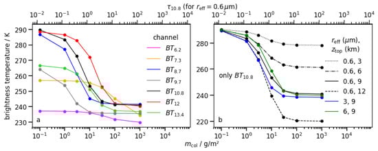
Figure 18.
Median brightness temperature of different SEVIRI channels averaged for 500 simulations (see text); (a) brightness temperatures for an ash cloud with and for different , (b) for different and .
Figure 19 shows combinations of different brightness temperatures and brightness temperature differences for the same simulations. The size of the markers encodes . Markers of constant and but different are connected by black, blue and violet lines for 0.6 μm, 3 μm and 6 μm, respectively, whereas the linestyle denotes . Additionally, points of constant , and variable are connected by red lines, and points of constant , and variable by green lines. Thus, Figure 19 shows whether the variation of different parameters leads to similar behaviors with respect to certain brightness temperatures (differences). Panel (a) shows against 10.8–12; this combination has often been studied [37,38]. For an increase in (along the black lines) reduces 10.8–12 and 10.8–12; the latter is related to the spectral dependence of the mass extinction coefficient of volcanic ash [3]. An increase in (along the red line) also reduces and leads overall to a similar change in this two-dimensional phase space, i.e., the black and the red curves are parallel and lie on top of each other. However, for the directions of these curves deviate as 10.8–12 vanishes if the ash cloud becomes opaque in the thermal infrared; thus, and can be distinguished. In (c), and are combined. Here the black and the red curve proceed in different directions already for and allow the separation of the influence of and : Increasing either of the two quantities reduces , but increasing changes and similarly, thus shows only minor changes. Yet, increasing leads to a reduction of , which is ~ 20 in the absence of volcanic ash due to the impact of carbon dioxide (see Figure 18), but vanishes as the ash cloud becomes opaque. In principle, the same behavior is visible for in (b) and (d), but the curves corresponding to different are located closer together. Note that for (violet curve) 10.8–12 is positive independent of for [3,38].
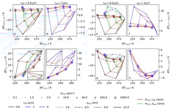
Figure 19.
Combinations of the medians of different brightness temperatures and brightness temperature differences, calculated from 500 simulations for each volcanic ash cloud (see text); mainly two different are used: (a,c,e,g) and 3 (b,d,f,h); is given by the size of the markers; markers with constant and but different are connected by black, blue and violet lines for 0.6 μm, 3 μm and 6 μm, respectively; the linestyle encodes ; points of constant , and variable are connected by red lines, and points of constant , and variable by green lines.
The variation of brightness temperatures (differences) due to is shown by the green lines as an example. In (a) and (c), cannot be determined easily as it is entangled with and . Therefore, we consider , and , which are located at the typical absorption peak of volcanic ash and which are influenced differently depending on the particle size [3]. Panel (e) shows against . Here mostly leads to , in contrast to 3 μm and 6 μm (except for , but even there the can be separated). Panel (g) shows on the y-axis. The blue curve for is convex, whereas the violet curve for is concave. A threshold at roughly with respect to would allow to separate the different except for . To summarize, it is possible to disentangle the physical quantities , and using the MSG/SEVIRI channels in the thermal infrared and exploiting the dependence of the mass extinction coefficient of volcanic ash on the wavelength and the particle size as well as the relatively constant impact of other atmospheric gases (e.g., carbon dioxide).
The actual working principles of ANNs are hard to determine. However, one can try to quantify the importance of the individual input features for each ANN and thereby deduce which physical principles are exploited and which functions might be implemented internally. Neglecting those features and retraining the ANNs might also allow to simplify the algorithms [39,40]. We define two metrics: The first, , is the relative contribution of the xth input neuron to the total weight between the input layer and the first hidden layer, defined as
for an input layer of n neurons, a first hidden layer of m neurons and the connecting weights [10]. The expectation is that the weights of unimportant features will vanish during training such that they have no impact on the calculation of the ANNs. However, in case of multiple hidden layers it might be possible that the impact of a feature significantly changes in the subsequent layers. Therefore, we consider a second metric: the relative change in loss, , when a feature is set to zero (simulating for all ) for the complete test data set, i.e.,
with being the loss (here the mean squared error for regressions and the categorical cross entropy for the classification) for the full test data set, whereas is the loss for the test data set when setting the xth input to zero. When dropping an unimportant feature should not change significantly, no matter whether it has vanishing weights already between the input and the first hidden layer or deeper in the network. However, dropping an important feature that is necessary for the calculation of the ANN will lead to a worse performance and, therefore, a larger loss .
Figure 20 shows and for all four ANNs and their input features. The two metrics quantitatively lead to different results. Whereas shows for all features always at least a small value, produces relatively large contrasts; thus, using it becomes more obvious whether an input is important or not. However, qualitatively both methods lead to similar pictures: For example, for the classification both metrics (a, b) indicate to be the most important of all brightness temperatures. Compared with the results of the other ANNs also the total column water and the total column water vapor appear to be important, and finally the viewing zenith angle.

Figure 20.
Two estimations of the feature importance: the relative contribution to the total weight at the 1st hidden layer (; a,c,e,g) and the relative change in loss (; b,d,f,h) (see text for definition) for all four ANNs and all input features, including the viewing zenith angle (), the hour of day (HOD) and the day of year (DOY); the loss function used for is is the mean squared error for regressions and the categorical cross entropy for classification; bars are alternately colored blue and light blue for better readability.
For the retrieval (c, d) only ash-loaded samples are considered, with being the most important channel. Furthermore, , and are prominent in both metrics. This is in agreement with the conclusions drawn from Figure 19. Compared to the retrievals of and also the total column water and water vapor have significant impact on (d); they might be used to take the corresponding atmospheric constituents into account. For the retrieval, (e) implies , , and to be the most important brightness temperatures, and furthermore and surprisingly the day of year variables have large metrics. However, generally the contrast is not very large between the features. (f) however points out , and . The importance of is again in agreement with the conclusions from Figure 19. The large values for show that the performance of the algorithm heavily depends on the accuracy of the retrieval. For the retrieval, (g) slightly highlights , , . From the auxiliary features the latitude, the cosine of the viewing zenith angle, and the ash-free temperatures , and stand out. Again, the contrast between features is overall small. Using (h) leads roughly to the same result but stresses the leading channels , , even more. The importance of these channels for the derivation of was also visible in Figure 19.
Let us focus on (b, d, f, h) now: From the auxiliary input features the total column water vapor and the total column water play a minor role in the retrieval of and a larger one for the classification; for height and effective radius retrievals they are unimportant. The latitude appears to be important mostly for the retrieval and the classification, and the skin temperature only for the classification. The land/sea mask, the total column ozone, the longitude, the day of year and the hour of day are rather negligible in all cases.
The metric was also derived for the input features of the cirrus cloud retrieval CiPS, which also consisted of several ANNs to derive, e.g., the cirrus optical depth or the cloud top height, trained using collocated SEVIRI and CALIOP measurements [10]. Comparing the results CiPS and VACOS shows similarities, e.g., in both cases the brightness temperatures play a dominant role, but the day of year and surface classifications are rather negligible. A noteworthy difference is that whereas the retrieval of CiPS mainly depends on latitude (as maximum cirrus cloud top height strongly depends thereon; thus, a statistical effect), our results show only a smaller dependence on this quantity.
Generally, the metrics support the observations made before in Figure 19, with the brightness temperatures having the major impact, whereas the auxiliary data seem to be of minor importance (even the skin temperature). The low values for the geographical coordinates imply that the ANNs do not learn the geography of the Earth as visible from SEVIRI. Similarly, the low values for the land/sea mask show that even this rough classification of the Earth’s surface remains unregarded. The low values for the times (day of year, hour of day) indicate that the ANNs do also not learn seasonal or diurnal variations. Reasons why the ANNs do not internalize those more evolved concepts might be a too small training data set, or they are just not helpful enough as the central physical quantities are rather obtained in the observations. For example, although the atmospheric state undergoes a seasonal variation, volcanic ash clouds are independent of them as volcanic eruptions can take place at any time of year. The hint that the ANNs do not learn the map indicates that the method might be applicable to other regions of the Earth (e.g., using GOES or Himawari satellites).
7. Conclusions
In a companion paper, we introduced a new algorithm to retrieve volcanic ash properties, i.e., a pixel classification, the cloud top height (), the effective particle radius () and (indirectly from the optical depth at , ) the mass column concentration () from MSG/SEVIRI data using artificial neural networks; it is called VACOS (Volcanic Ash Cloud properties Obtained from SEVIRI [2]). The input data encompass the seven brightness temperatures of the imager’s channels in the thermal infrared and additional data from ECMWF. VACOS allows spatially and temporally highly resolved retrievals of volcanic ash clouds independent of daylight.
For the validation, VACOS is compared to independent measurements. With respect to CALIOP retrievals of the Puyehue-Cordón Caulle ash clouds (2011), VACOS shows quite a large variability on a single pixel basis. A regional average over pixels reduces this variability and leads to lower deviations between of VACOS and the lidar retrieval: the mean absolute percentage error (MAPE) of decreases to 45% and the MAPE of is 18% when considering only samples with a lidar retrieval of . Therefore, this averaging is recommended for future applications of the new algorithm. The VACOS-derived is in good agreement with the CALIOP measurements in most, but not all, cases. Deviations are generally within the uncertainties of the reference data. and by VACOS have the correct order of magnitude but exhibit significant scattering, with being slightly underestimated (having a mean percentage error of %), whereas lies within the regime constrained by literature values. The four category classification of VACOS detects the volcanic ash clouds with the highest mass loads, but ash layers with less than ~0.4 g m−2 are often misclassified as meteorological clouds (which includes liquid and ice water clouds). Similarly, SEVIRI images indicate that clear sky might be too often misclassified as cloudy, but here dedicated retrievals of meteorological clouds should provide help. Additionally considering a cirrus retrieval also shows that thick ice clouds have the potential to completely hide the volcanic ash or distort their retrieval; thus, we also recommend to consider VACOS results always together with a cirrus cloud retrieval to avoid misinterpretations.
As another reference, airborne lidar and in situ data of an Eyjafjallajökull ash cloud (2010) are used as obtained during two different measurement campaigns by FAAM and DLR, respectively. The various measurement results for , and agree well, considering that different instrumentation was used and different parts of the ash cloud were probed. Main differences are a higher upper estimate of according to the DLR (roughly 2 g m−2 compared to mostly around 1 g m−2) and a higher upper limit for in the FAAM data (2 compared to 1 ); estimates are up to ~6 in both cases. For the most part, the VACOS retrievals of and lie within the uncertainty intervals of the airborne measurements, whereas from the new retrieval scatters around the reference values with deviations in the order of 1– 2 . Concurrent overestimations of and can be explained by low in some cases, but not generally. The classification algorithm correctly detects the ash cloud.
Results of a volcanic ash transport and dispersion multi model multi source term ensemble simulating the eruption of Eyjafjallajökull (2010) are used to analyze the performance of VACOS on large scales. Different accumulation rules are investigated when regridding the satellite retrievals. Example scenes indicate that the model results and the VACOS retrievals are in good agreement close to the volcano, but that there are displacements of the ash clouds at larger distances, e.g., for ash clouds above continental Europe; those might be caused by inaccuracies in the model calculations. As a consequence, distance offsets up to 100 are considered. The model ensemble covers a larger interval of possible than VACOS: can be an order of magnitude larger in the model calculations than in the VACOS retrieval in a surrounding of some 100 around the vent, whereas it can be more than one order of magnitude smaller at distances of >1000 . Considering only samples with according to both the model ensemble and VACOS results in a MAPE of ~60% for of VACOS.
To further quantify the performance of VACOS, a simulated test data set similar to its training data is used. The four category classification classifies correctly more than 94% of the simulated cases, except when both volcanic ash and meteorological clouds are present, which reduces the amount of correct classifications to ~50%. Simplifying classification results to a binary ash flag results in a probability of detection (POD) of close to 100%. The retrievals of , and have mostly MAPEs of 10–100%. For , the MAPE is ~40% or less for ash layers with a true of 0.1 (corresponding to of 0.3–0.7 g m−2) or more; the retrieval error of is up to ~10% for ash layers above 5 ; and has an error of up to 35% for true radii of 0.6–6 . The performance increases with increasing and of the ash layers. Thus, the greatest errors occur for the thinnest and lowest ash clouds, for which the MAPE can even exceed 100%. No significant differences exist between underlying land and sea surfaces, in contrast to the presence of meteorological clouds (particularly if they are located above the ash layer), which can increase the MAPE by up to one order of magnitude and decrease the POD by a factor of two. Analysis of the geographical dependence shows that deserts lead to a decreased performance for clear sky cases, e.g., the accuracy of the binary ash flag slightly decreases (ca. 1%), whereas the MAPE for increases. An increased performance of the binary ash flag is observable in the presence of clouds above areas that are typically cloudy, i.e., where many cloudy samples are included in the simulated (training and test) data sets. The retrievals of and show increased MAPEs with increasing viewing zenith angle, whereas the MAPE of increases with the absolute latitude. Using further simulated test data sets, the dependence of the retrievals with respect to the ash layer(s) is investigated. The (unretrieved) geometrical layer thickness and the presence of multiple layers might introduce errors of about 30% for , 5% for , but are negligible for .
Volcanic ash detection can be performed using the binary ash flag or / and corresponding thresholds. Using the simulated data shows that the detection ability of the binary ash flag is better than the one using , and both outperform the usage of the brightness temperature difference between the channels centered at and 12 ; using for a threshold of 0.2 g m−2 and considering only ash layers with 0.2–1 g m−2 leads to a POD of more than 90% and a false alarm rate (FAR) of ca. 1%. For the CALIOP data, higher PODs can be found when using compared to the binary ash flag; a similar threshold as before leads to a POD of ~70%. Using the model results as reference data, we find for similar thresholds PODs of 20–85% and FARs of 0.3–3%, which strongly depend on the accumulation rule and the allowed distance offsets. Note that the model result is not a perfect representation of reality; therefore, POD and FAR should be regarded as metrics quantifying the agreement of model and retrieval results rather than performance metrics attributed exclusively to VACOS.
VACOS is also compared to its direct predecessor VADUGS. The latter exhibits a better detection performance on the CALIOP data and has a smaller FAR for the model data, but it also misses significantly more modeled ash clouds than VACOS, especially also ash plumes close to the vent. Whereas the retrieval of VADUGS performs similar to VACOS for the CALIOP data, it underestimates compared to the airborne lidar and in situ findings. The VADUGS retrieval of is reliable only for ash clouds with of the order 1 g m−2 or larger. Overall, VADUGS seems much more sensitive to specific cases than VACOS. In the end, we consider the importance of different input features of the VACOS retrievals, showing that they are mostly dependent on the SEVIRI brightness temperatures, and partly also on the viewing zenith angle as well as total column water and water vapor estimates from ECMWF. Longitude, land/sea-mask and times have negligible impact on the output.
In the future it would be desirable to further analyze the retrieval performance also with respect to mineral dust. As volcanic ash and mineral dust share similar optical properties due to the common high silica content, it is likely that VACOS might misclassify dust as volcanic ash [7,41,42]. In this case, it would be interesting to see if VACOS could be used to retrieve dust cloud properties as well. The aviation industry considers similar risks for volcanic ash and for dust, hence a combined retrieval seems advantageous. Furthermore, VACOS has been tailored for Meteosat-9/MSG2. The usage of the retrieval algorithm with the currently operational MSG satellite as well as the satellites in other operation modes (i.e., rapid scan mode, Indian Ocean data coverage) should be investigated. As other infrared imagers aboard geostationary weather satellites such as GOES-R [43], Himawari-8/9 [44] and Fengyun-4A [45] share similar channels with MSG/SEVIRI one could also investigate the transferability of VACOS to those instruments. The error of the VACOS retrievals decreases when a local average is calculated. To expand on this idea, further processing of the retrieval map seems desirable, e.g., to cluster ash-containing pixels and quantify the resulting ash patches, or even track them in time. Possible fields of application of VACOS include the Volcanic Ash Advisory Centers, the intercomparison with other volcanic ash retrievals (as in [46]), calibrating and validating volcanic ash transport and dispersion models [35,47,48,49] and flight planning for future in situ measurements [15]. Due to the high spatial and temporal resolution, it can be used to track individual ash clouds to investigate their lifecycle on timespans of days to weeks. In combination with information on liquid and ice water clouds, aerosol-cloud interaction could be analyzed.
In summary, VACOS is well characterized and shown to be reliably applicable under different atmospheric conditions and for various kinds of volcanic ash clouds. It can be utilized for atmospheric research as well as for air space monitoring with respect to volcanic ash. Operational use by the German weather service (DWD) as a follow-on of VADUGS is planned.
Author Contributions
Conceptualization, D.P. and L.B.; methodology, D.P.; software, D.P.; validation, D.P.; formal analysis, D.P.; investigation, D.P.; data sources, J.K., U.S., F.M., M.P. and L.B.; writing—original draft preparation, D.P.; writing—review and editing, L.B., C.V., J.K., U.S., F.M. and M.P.; visualization, D.P.; supervision, L.B. and C.V.; project administration, L.B.; funding acquisition, C.V. and L.B. All authors have read and agreed to the published version of the manuscript.
Funding
D. Piontek and L. Bugliaro were supported by the European Unions’s Horizon 2020 research and innovation program under grant agreement No. 723986 (EUNADICS-AV). C. Voigt acknowledges funding by the Helmholtz Association under contract HGF W2/W3-60.
Institutional Review Board Statement
Not applicable.
Informed Consent Statement
Not applicable.
Data Availability Statement
Data presented in this study is available on request from the corresponding author.
Acknowledgments
The MSG/SEVIRI data were provided by EUMETSAT (European Organisation for the Exploitation of Meteorological Satellites) and the auxiliary data were obtained from ECMWF (European Center for Medium-Range Weather Forecasts). Radiative transfer calculations have been performed on DLR’s CARA (Deutsches Zentrum für Luft- und Raumfahrt; Cluster for Advanced Research in Aerospace). Airborne data were obtained by DLR using the Falcon 20E, operated by DLR flight experiment facilities, and using the BAe-146-301 Atmospheric Research Aircraft which in 2010 was operated by Directflight Ltd. and managed by FAAM (Facility for Airborne Atmospheric Measurements), a joint entity of NERC (Natural Environment Research Council) and the Met Office. Furthermore, we like to thank M. Vázquez-Navarro, J. Strandgren, B. Mayer and M. Rapp for constructive discussions and valuable feedback, W. Beer for technical support, as well as J. Wilzewski and two reviewers for the helpful comments to improve the manuscript. J. Kar acknowledges useful discussions with M. Vaughan on correcting the low bias from the default ash lidar ratios used in CALIOP version 4.10.
Conflicts of Interest
The authors declare no conflict of interest.
Appendix A. Metrics
Different error metrics are used in this work, derived from a set of n pairs of retrieved values and corresponding true values . The mean squared error is defined as
The mean absolute percentage error is calculated by
The mean percentage error is
To quantify the performance of a boolean retrieval we consider the probability of detection and the false alarm rate (also probability of false detection [50])
with being the number of true positives (here meaning that the retrieval signals the presence of volcanic ash, which is really present), the false positives (presence of ash is signaled although none is present), the true negatives (absence of of ash is signaled and none is present) and the false negatives (absence of ash is signaled although it is present). The performance of multi-category classifications is described by the accuracy given as the number of correctly classified samples divided by the total number of samples. For two categories, the accuracy simplifies to
and if no negative samples are present, i.e., , the accuracy equals the POD.
Appendix B. Π-Sigmoid Distribution
The -sigmoid distribution was introduced by Alivanoglou and Likas [18] and is defined as the difference of two sigmoid functions, i.e.,
with a and parameterizing the positions of the rise of the corresponding sigmoid, and describing their steepness. The expectation value is and for the the standard deviation holds
References
- Bugliaro, L.; Piontek, D.; Kox, S.; Schmidl, M.; Mayer, B.; Müller, R.; Vázquez-Navarro, M.; Gasteiger, J.; Kar, J. Combining radiative transfer calculations and a neural network for the remote sensing of volcanic ash using MSG/SEVIRI. 2021; in preparation. [Google Scholar]
- Piontek, D.; Bugliaro, L.; Schmidl, M.; Zhou, D.K.; Voigt, C. The New Volcanic Ash Retrieval VACOS Using MSG/SEVIRI and Artificial Neural Networks: 1. Development. Remote Sens. 2021, 13, 3112. [Google Scholar] [CrossRef]
- Piontek, D.; Hornby, A.; Voigt, C.; Bugliaro, L.; Gasteiger, J. Determination of complex refractive indices and optical properties of volcanic ashes in the thermal infrared based on generic petrological compositions. J. Volcanol. Geotherm. Res. 2021, 411, 107174. [Google Scholar] [CrossRef]
- Zhou, D.K.; Larar, A.M.; Liu, X.; Smith, W.L.; Strow, L.L.; Yang, P.; Schlüssel, P.; Calbet, X. Global Land Surface Emissivity Retrieved From Satellite Ultraspectral IR Measurements. IEEE Trans. Geosci. Remote Sens. 2011, 49, 1277–1290. [Google Scholar] [CrossRef]
- Zhou, D.K.; Larar, A.M.; Liu, X. MetOp-A/IASI Observed Continental Thermal IR Emissivity Variations. IEEE J. Sel. Top. Appl. Earth Obs. Remote Sens. 2013, 6, 1156–1162. [Google Scholar] [CrossRef]
- Zhou, D.K.; Larar, A.M.; Liu, X. On the relationship between land surface infrared emissivity and soil moisture. J. Appl. Remote Sens. 2018, 12, 1–14. [Google Scholar] [CrossRef] [Green Version]
- Watkin, S.C. The application of AVHRR data for the detection of volcanic ash in a Volcanic Ash Advisory Centre. Meteorol. Appl. 2003, 10, 301–311. [Google Scholar] [CrossRef]
- Kaufman, Y.J.; Koren, I.; Remer, L.A.; Rosenfeld, D.; Rudich, Y. The effect of smoke, dust, and pollution aerosol on shallow cloud development over the Atlantic Ocean. Proc. Natl. Acad. Sci. USA 2005, 102, 11207–11212. [Google Scholar] [CrossRef] [PubMed] [Green Version]
- Strandgren, J.; Bugliaro, L.; Sehnke, F.; Schröder, L. Cirrus cloud retrieval with MSG/SEVIRI using artificial neural networks. Atmos. Meas. Tech. 2017, 10, 3547–3573. [Google Scholar] [CrossRef] [Green Version]
- Strandgren, J.; Fricker, J.; Bugliaro, L. Characterisation of the artificial neural network CiPS for cirrus cloud remote sensing with MSG/SEVIRI. Atmos. Meas. Tech. 2017, 10, 4317–4339. [Google Scholar] [CrossRef] [Green Version]
- Thomas, G.E.; Stamnes, K. Radiative Transfer in the Atmosphere and Ocean, 1st ed.; Cambridge University Press: New York, NY, USA, 2002. [Google Scholar]
- de Laat, A.; Vazquez-Navarro, M.; Theys, N.; Stammes, P. Analysis of properties of the 19 February 2018 volcanic eruption of Mount Sinabung in S5P/TROPOMI and Himawari-8 satellite data. Nat. Hazards Earth Syst. Sci. 2020, 20, 1203–1217. [Google Scholar] [CrossRef]
- Schneider, D.J.; Van Eaton, A.R.; Wallace, K.L. Satellite observations of the 2016–2017 eruption of Bogoslof volcano: Aviation and ash fallout hazard implications from a water-rich eruption. Bull. Volcanol. 2020, 82, 29. [Google Scholar] [CrossRef]
- Deguine, A.; Petitprez, D.; Clarisse, L.; Guđmundsson, S.; Outes, V.; Villarosa, G.; Herbin, H. Complex refractive index of volcanic ash aerosol in the infrared, visible, and ultraviolet. Appl. Opt. 2020, 59, 884–895. [Google Scholar] [CrossRef]
- Schumann, U.; Weinzierl, B.; Reitebuch, O.; Schlager, H.; Minikin, A.; Forster, C.; Baumann, R.; Sailer, T.; Graf, K.; Mannstein, H.; et al. Airborne observations of the Eyjafjalla volcano ash cloud over Europe during air space closure in April and May 2010. Atmos. Chem. Phys. 2011, 11, 2245–2279. [Google Scholar] [CrossRef] [Green Version]
- Marenco, F.; Johnson, B.; Turnbull, K.; Newman, S.; Haywood, J.; Webster, H.; Ricketts, H. Airborne lidar observations of the 2010 Eyjafjallajökull volcanic ash plume. J. Geophys. Res. Atmos. 2011, 116. [Google Scholar] [CrossRef]
- Turnbull, K.; Johnson, B.; Marenco, F.; Haywood, J.; Minikin, A.; Weinzierl, B.; Schlager, H.; Schumann, U.; Leadbetter, S.; Woolley, A. A case study of observations of volcanic ash from the Eyjafjallajökull eruption: 1. In situ airborne observations. J. Geophys. Res. Atmos. 2012, 117. [Google Scholar] [CrossRef] [Green Version]
- Alivanoglou, A.; Likas, A. Probabilistic Models Based on the Π-Sigmoid Distribution. In Artificial Neural Networks in Pattern Recognition; Prevost, L., Marinai, S., Schwenker, F., Eds.; Springer: Berlin/Heidelberg, Germany, 2008; pp. 36–43. [Google Scholar]
- Typical Radiometric Noise, Calibration Bias and Stability for Meteosat-8, -9, -10 and -11 SEVIRI. European Organisation for the Exploitation of Meteorological Satellites. 2019. Available online: https://www-cdn.eumetsat.int/files/2020-04/pdf_typ_radiomet_acc_msg-1-2.pdf (accessed on 5 August 2021).
- Winker, D.M.; Vaughan, M.A.; Omar, A.; Hu, Y.; Powell, K.A.; Liu, Z.; Hunt, W.H.; Young, S.A. Overview of the CALIPSO Mission and CALIOP Data Processing Algorithms. J. Atmos. Ocean. Technol. 2009, 26, 2310–2323. [Google Scholar] [CrossRef]
- Kim, M.H.; Omar, A.H.; Tackett, J.L.; Vaughan, M.A.; Winker, D.M.; Trepte, C.R.; Hu, Y.; Liu, Z.; Poole, L.R.; Pitts, M.C.; et al. The CALIPSO version 4 automated aerosol classification and lidar ratio selection algorithm. Atmos. Meas. Tech. 2018, 11, 6107–6135. [Google Scholar] [CrossRef] [PubMed] [Green Version]
- Gasteiger, J.; Groß, S.; Freudenthaler, V.; Wiegner, M. Volcanic ash from Iceland over Munich: Mass concentration retrieved from ground-based remote sensing measurements. Atmos. Chem. Phys. 2011, 11, 2209–2223. [Google Scholar] [CrossRef] [Green Version]
- Winker, D.M.; Liu, Z.; Omar, A.; Tackett, J.; Fairlie, D. CALIOP observations of the transport of ash from the Eyjafjallajökull volcano in April 2010. J. Geophys. Res. Atmos. 2012, 117. [Google Scholar] [CrossRef]
- Bignami, C.; Corradini, S.; Merucci, L.; de Michele, M.; Raucoules, D.; De Astis, G.; Stramondo, S.; Piedra, J. Multisensor Satellite Monitoring of the 2011 Puyehue-Cordon Caulle Eruption. IEEE J. Sel. Top. Appl. Earth Obs. Remote Sens. 2014, 7, 2786–2796. [Google Scholar] [CrossRef]
- Ishimoto, H.; Hayashi, M.; Mano, Y. Optimal ash particle refractive index model for simulating the brightness temperature spectrum of volcanic ash clouds from satellite infrared sounder measurements. Atmos. Meas. Tech. Discuss. 2021, 2021, 1–28. [Google Scholar] [CrossRef]
- Debling, F.; Schneider, J.F.; Rosi, M.; Leoz-Garziandia, E.; Rorije, E. Technical Cooperation Mission, Effects of the Puyehue-Cordón Caulle Eruption Argentina, 4–19 July 2011. Joint UNEP/OCHA Environment Unit, 2011. Available online: https://www.eecentre.org/wp-content/uploads/2019/06/Argentina-volcan-eruption-2011-report.pdf (accessed on 5 August 2021).
- Botto, I.L.; Canafoglia, M.E.; Gazzoli, D.; González, M.J. Spectroscopic and Microscopic Characterization of Volcanic Ash from Puyehue-(Chile) Eruption: Preliminary Approach for the Application in the Arsenic Removal. J. Spectrosc. 2013, 2013, 254517. [Google Scholar] [CrossRef] [Green Version]
- Johnson, B.; Turnbull, K.; Brown, P.; Burgess, R.; Dorsey, J.; Baran, A.J.; Webster, H.; Haywood, J.; Cotton, R.; Ulanowski, Z.; et al. In situ observations of volcanic ash clouds from the FAAM aircraft during the eruption of Eyjafjallajökull in 2010. J. Geophys. Res. Atmos. 2012, 117. [Google Scholar] [CrossRef] [Green Version]
- Ball, J.G.C.; Reed, B.E.; Grainger, R.G.; Peters, D.M.; Mather, T.A.; Pyle, D.M. Measurements of the complex refractive index of volcanic ash at 450, 546.7, and 650 nm. J. Geophys. Res. Atmos. 2015, 120, 7747–7757. [Google Scholar] [CrossRef]
- Weber, K.; Eliasson, J.; Vogel, A.; Fischer, C.; Pohl, T.; van Haren, G.; Meier, M.; Grobéty, B.; Dahmann, D. Airborne in situ investigations of the Eyjafjallajökull volcanic ash plume on Iceland and over north-western Germany with light aircrafts and optical particle counters. Atmos. Environ. 2012, 48, 9–21. [Google Scholar] [CrossRef]
- Gudmundsson, M.T.; Thordarson, T.; Höskuldsson, A.; Larsen, G.; Björnsson, H.; Prata, F.J.; Oddsson, B.; Magnússon, E.; Högnadóttir, T.; Petersen, G.N.; et al. Ash generation and distribution from the April-May 2010 eruption of Eyjafjallajökull, Iceland. Sci. Rep. 2012, 2, 572. [Google Scholar] [CrossRef] [Green Version]
- Rose, W.; Gu, Y.; Watson, I.; Yu, T.; Blut, G.; Prata, A.; Krueger, A.; Krotkov, N.; Carn, S.; Fromm, M.; et al. The February–March 2000 Eruption of Hekla, Iceland from a Satellite Perspective. In Volcanism and the Earth’s Atmosphere; American Geophysical Union: Washington, DC, USA, 2004; pp. 107–132. [Google Scholar] [CrossRef] [Green Version]
- Rose, W.I.; Bluth, G.J.S.; Watson, I.M. Ice in Volcanic Clouds: When and Where? In Proceedings of the 2nd International Conference on Volcanic Ash and Aviation Safety, Alexandria, VA, USA, 21–24 June 2004; Office of the Federal Coordinator for Meteorological Services and Supporting Research: Silver Spring, MD, USA, 2004; pp. 3.27–3.33. [Google Scholar]
- Durant, A.J.; Shaw, R.A.; Rose, W.I.; Mi, Y.; Ernst, G.G.J. Ice nucleation and overseeding of ice in volcanic clouds. J. Geophys. Res. Atmos. 2008, 113. [Google Scholar] [CrossRef] [Green Version]
- Plu, M.; Scherllin-Pirscher, B.; Arnold Arias, D.; Baro, R.; Bigeard, G.; Bugliaro, L.; Carvalho, A.; El Amraoui, L.; Eschbacher, K.; Hirtl, M.; et al. A tailored multi-model ensemble for air traffic management: Demonstration and evaluation for the Eyjafjallajökull eruption in May 2010. Nat. Hazards Earth Syst. Sci. Discuss. 2021, 2021, 1–32. [Google Scholar] [CrossRef]
- Kox, S.; Bugliaro, L.; Ostler, A. Retrieval of cirrus cloud optical thickness and top altitude from geostationary remote sensing. Atmos. Meas. Tech. 2014, 7, 3233–3246. [Google Scholar] [CrossRef] [Green Version]
- Prata, A.J. Infrared radiative transfer calculations for volcanic ash clouds. Geophys. Res. Lett. 1989, 16, 1293–1296. [Google Scholar] [CrossRef]
- Wen, S.; Rose, W.I. Retrieval of sizes and total masses of particles in volcanic clouds using AVHRR bands 4 and 5. J. Geophys. Res. Atmos. 1994, 99, 5421–5431. [Google Scholar] [CrossRef]
- LeCun, Y.; Denker, J.S.; Solla, S.A. Optimal Brain Damage. In Advances in Neural Information Processing Systems 2; Touretzky, D.S., Ed.; Morgan-Kaufmann: San Francisco, CA, USA, 1990; pp. 598–605. [Google Scholar]
- Piscini, A.; Carboni, E.; Del Frate, F.; Grainger, R.G. Simultaneous retrieval of volcanic sulphur dioxide and plume height from hyperspectral data using artificial neural networks. Geophys. J. Int. 2014, 198, 697–709. [Google Scholar] [CrossRef] [Green Version]
- Ackerman, S.A. Remote sensing aerosols using satellite infrared observations. J. Geophys. Res. Atmos. 1997, 102, 17069–17079. [Google Scholar] [CrossRef]
- Gray, T.M.; Bennartz, R. Automatic volcanic ash detection from MODIS observations using a back-propagation neural network. Atmos. Meas. Tech. 2015, 8, 5089–5097. [Google Scholar] [CrossRef] [Green Version]
- Schmit, T.J.; Gunshor, M.M.; Menzel, W.P.; Gurka, J.J.; Li, J.; Bachmeier, A.S. Introducing the Next-Generation Advanced Baseline Imager on GOES-R. Bull. Am. Meteorol. Soc. 2005, 86, 1079–1096. [Google Scholar] [CrossRef]
- Bessho, K.; Date, K.; Hayashi, M.; Ikeda, A.; Imai, T.; Inoue, H.; Kumagai, Y.; Miyakawa, T.; Murata, H.; Ohno, T.; et al. An Introduction to Himawari-8/9 - Japan’s New-Generation Geostationary Meteorological Satellites. J. Meteorol. Soc. Jpn. Ser. II 2016, 94, 151–183. [Google Scholar] [CrossRef] [Green Version]
- Yang, J.; Zhang, Z.; Wei, C.; Lu, F.; Guo, Q. Introducing the New Generation of Chinese Geostationary Weather Satellites, Fengyun-4. Bull. Am. Meteorol. Soc. 2017, 98, 1637–1658. [Google Scholar] [CrossRef]
- Meeting on the Intercomparison of Satellite-Based Volcanic Ash Retrieval Algorithms, Madison WI, USA, 29 June–2 July 2015, Final Report. World Meteorological Organization, 2015. Available online: https://web.archive.org/web/20171113102551/http://www.wmo.int/pages/prog/sat/documents/SCOPE-NWC-PP2_VAIntercompWSReport2015.pdf (accessed on 5 August 2021).
- Stohl, A.; Prata, A.J.; Eckhardt, S.; Clarisse, L.; Durant, A.; Henne, S.; Kristiansen, N.I.; Minikin, A.; Schumann, U.; Seibert, P.; et al. Determination of time- and height-resolved volcanic ash emissions and their use for quantitative ash dispersion modeling: The 2010 Eyjafjallajökull eruption. Atmos. Chem. Phys. 2011, 11, 4333–4351. [Google Scholar] [CrossRef] [Green Version]
- Dacre, H.F.; Harvey, N.J.; Webley, P.W.; Morton, D. How accurate are volcanic ash simulations of the 2010 Eyjafjallajökull eruption? J. Geophys. Res. Atmos. 2016, 121, 3534–3547. [Google Scholar] [CrossRef] [Green Version]
- Plu, M.; Bigeard, G.; Sič, B.; Emili, E.; Bugliaro, L.; El Amraoui, L.; Guth, J.; Josse, B.; Mona, L.; Piontek, D. Modelling the volcanic ash plume from Eyjafjallajökull eruption (May 2010) over Europe: Evaluation of the benefit of source term improvements and of the assimilation of aerosol measurements. Nat. Hazards Earth Syst. Sci. Discuss. 2021, 2021, 1–24. [Google Scholar] [CrossRef]
- Barnes, L.R.; Schultz, D.M.; Gruntfest, E.C.; Hayden, M.H.; Benight, C.C. CORRIGENDUM: False Alarm Rate or False Alarm Ratio? Weather Forecast. 2009, 24, 1452–1454. [Google Scholar] [CrossRef] [Green Version]
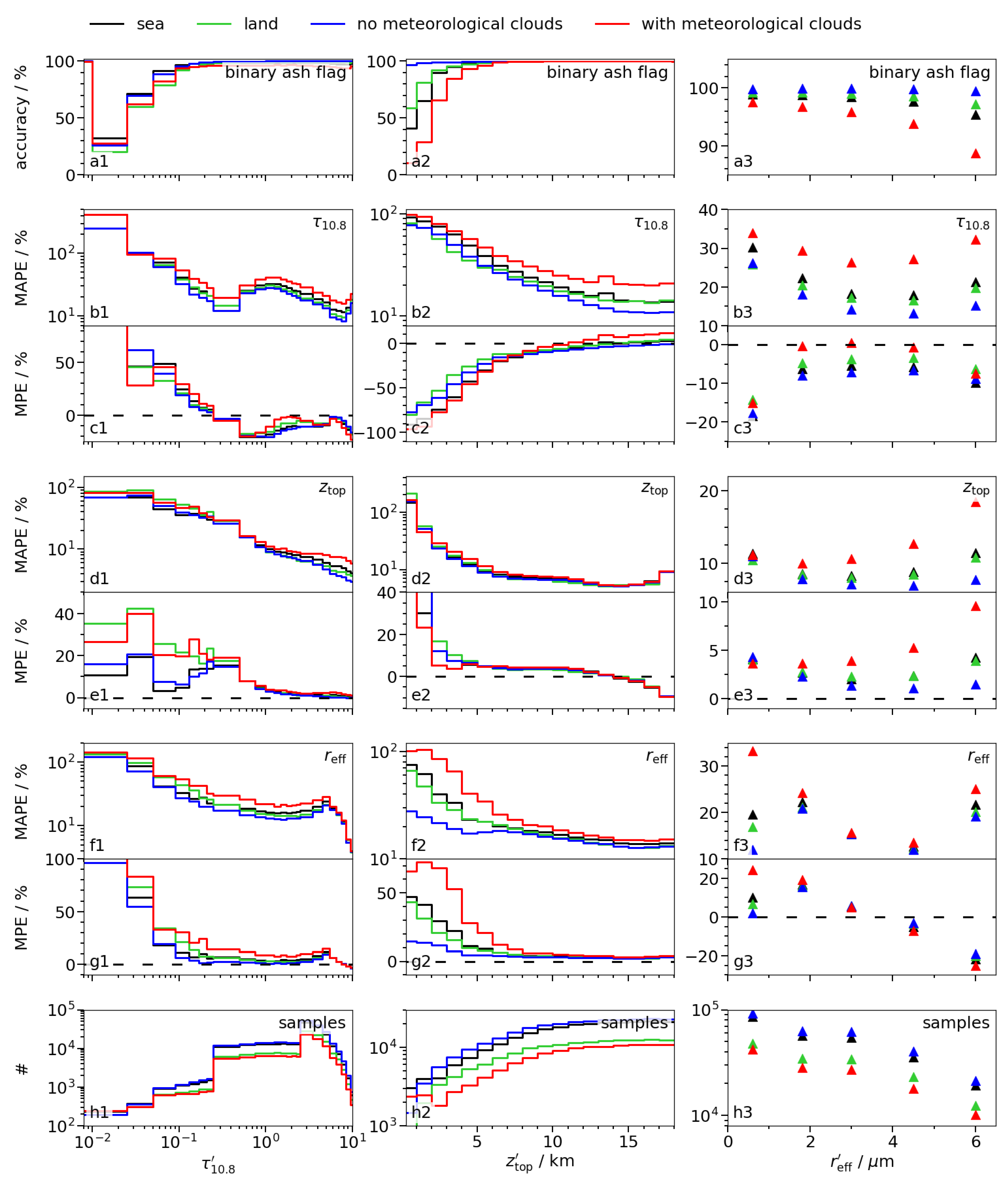
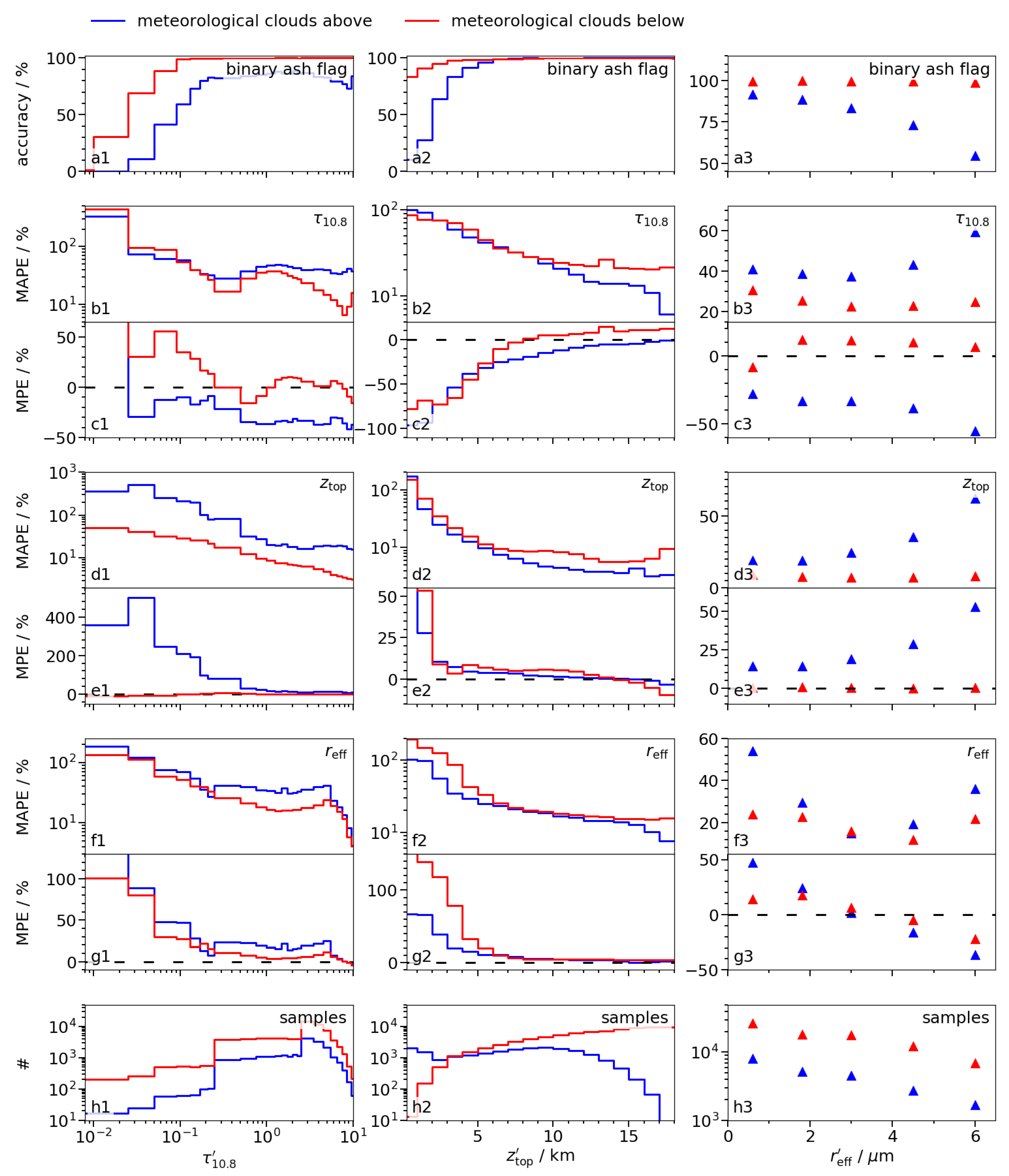
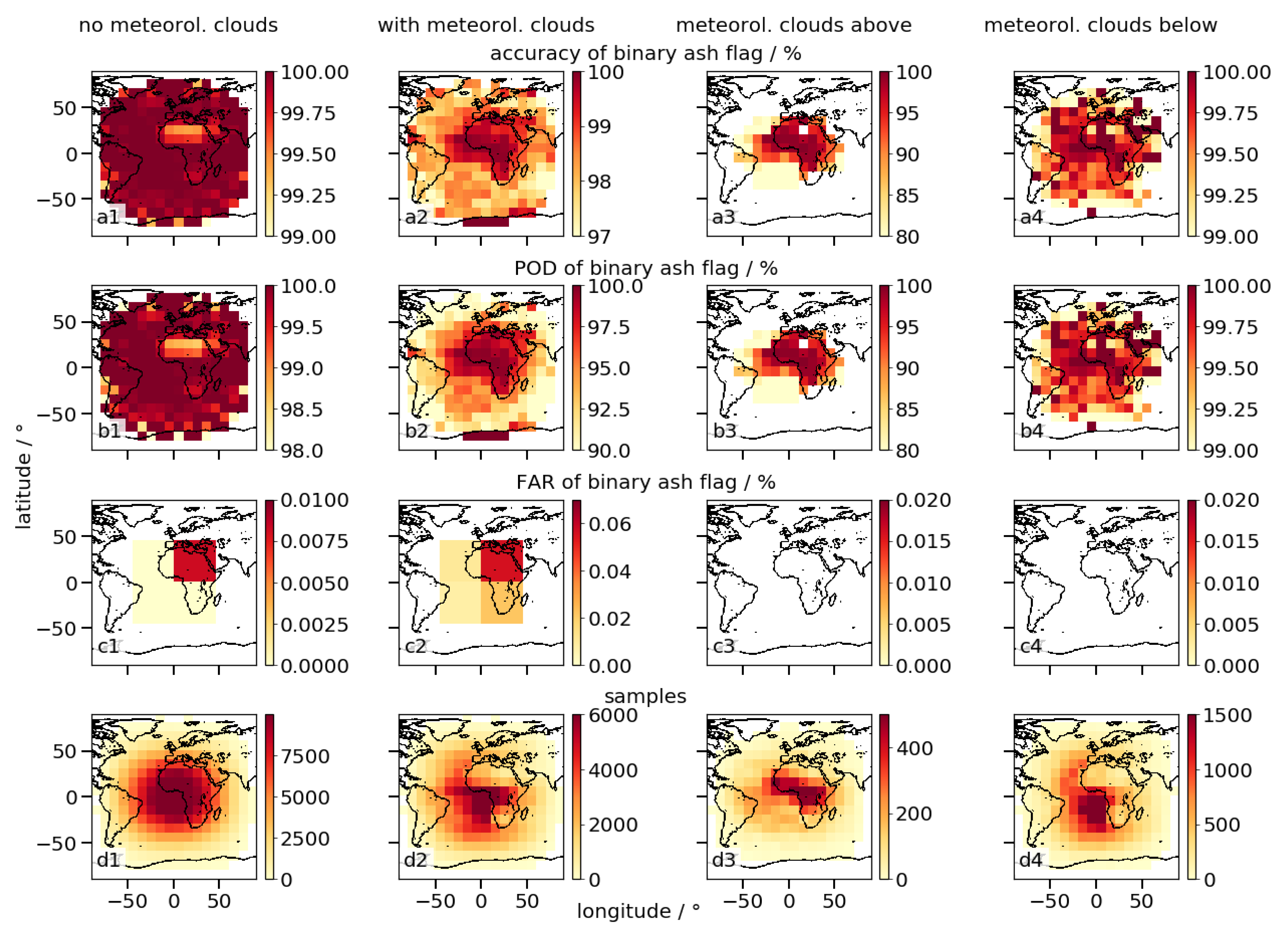
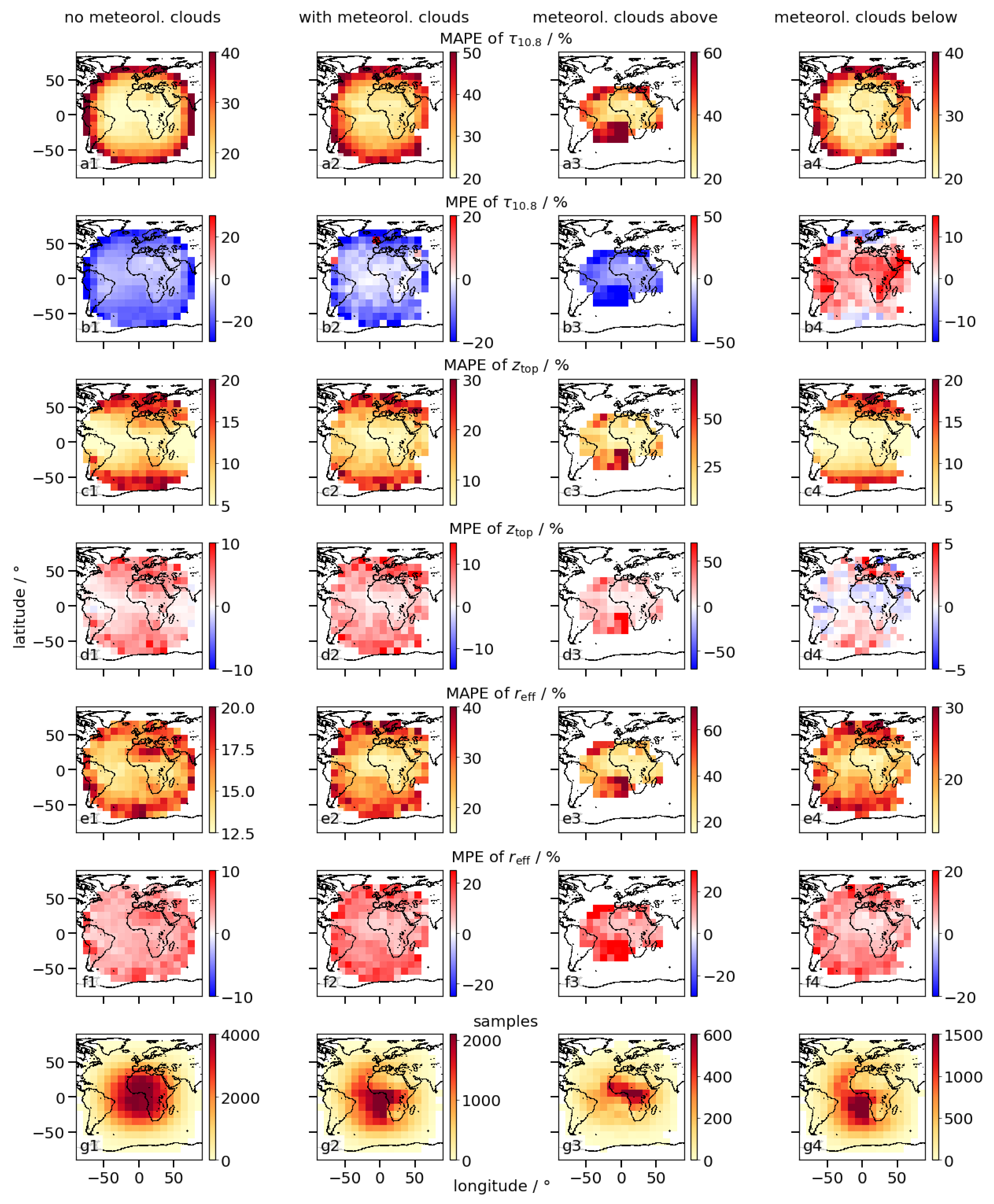
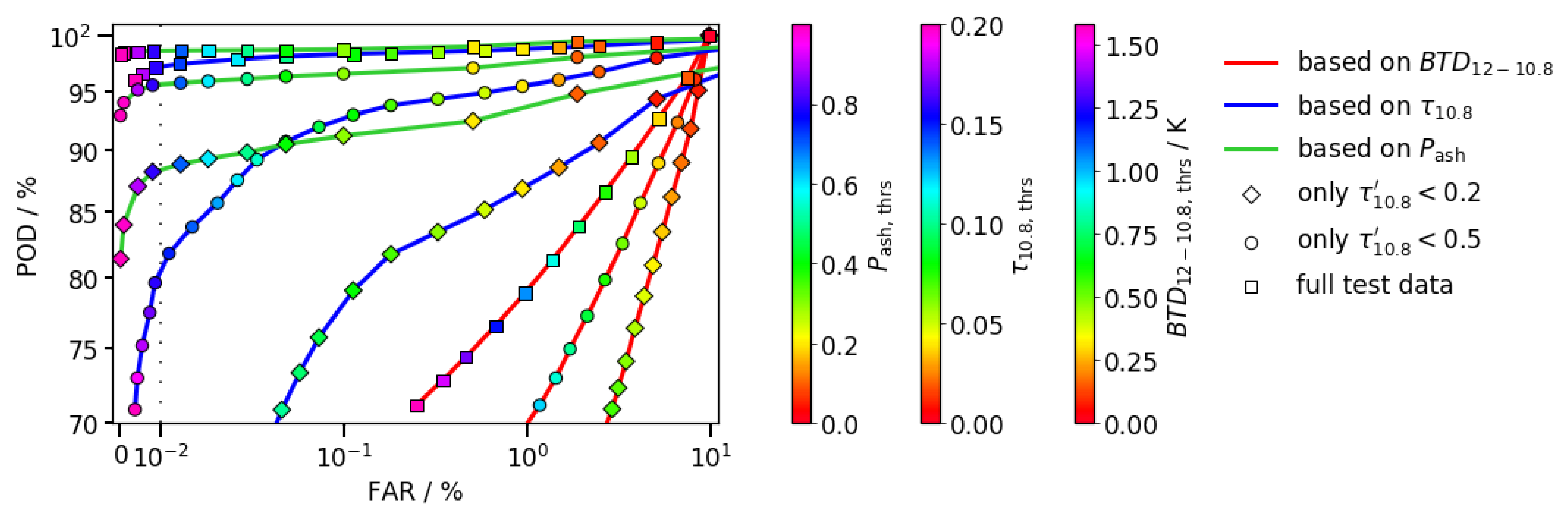
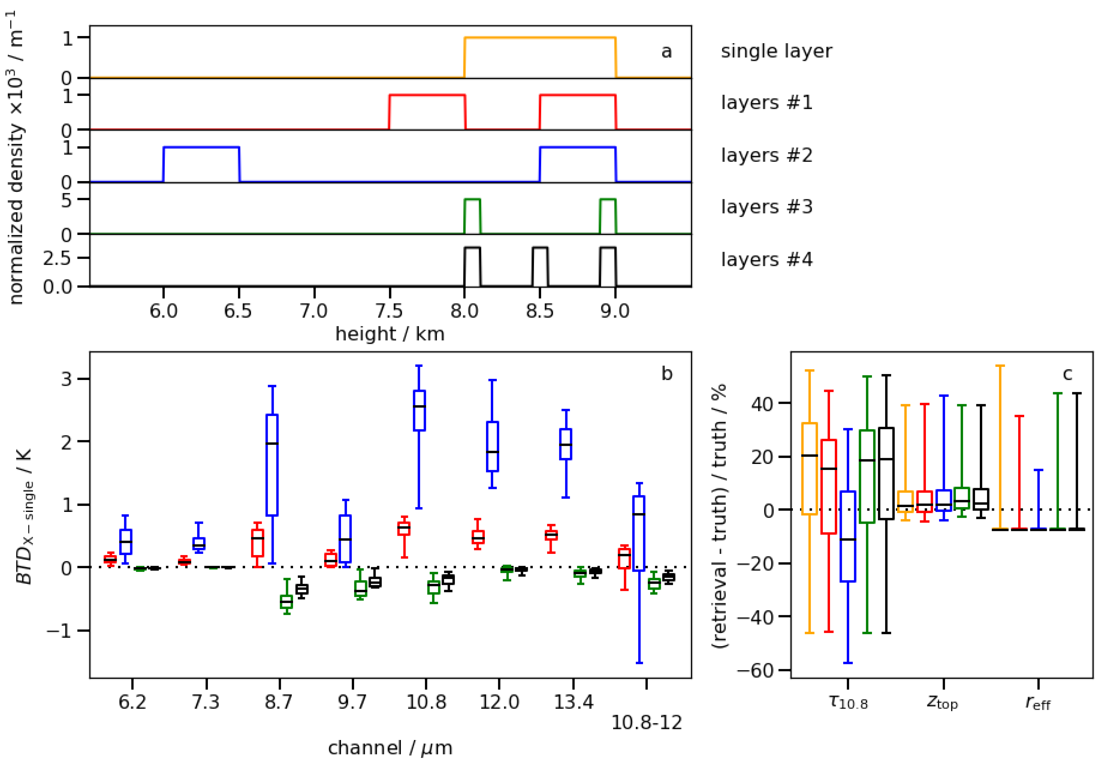
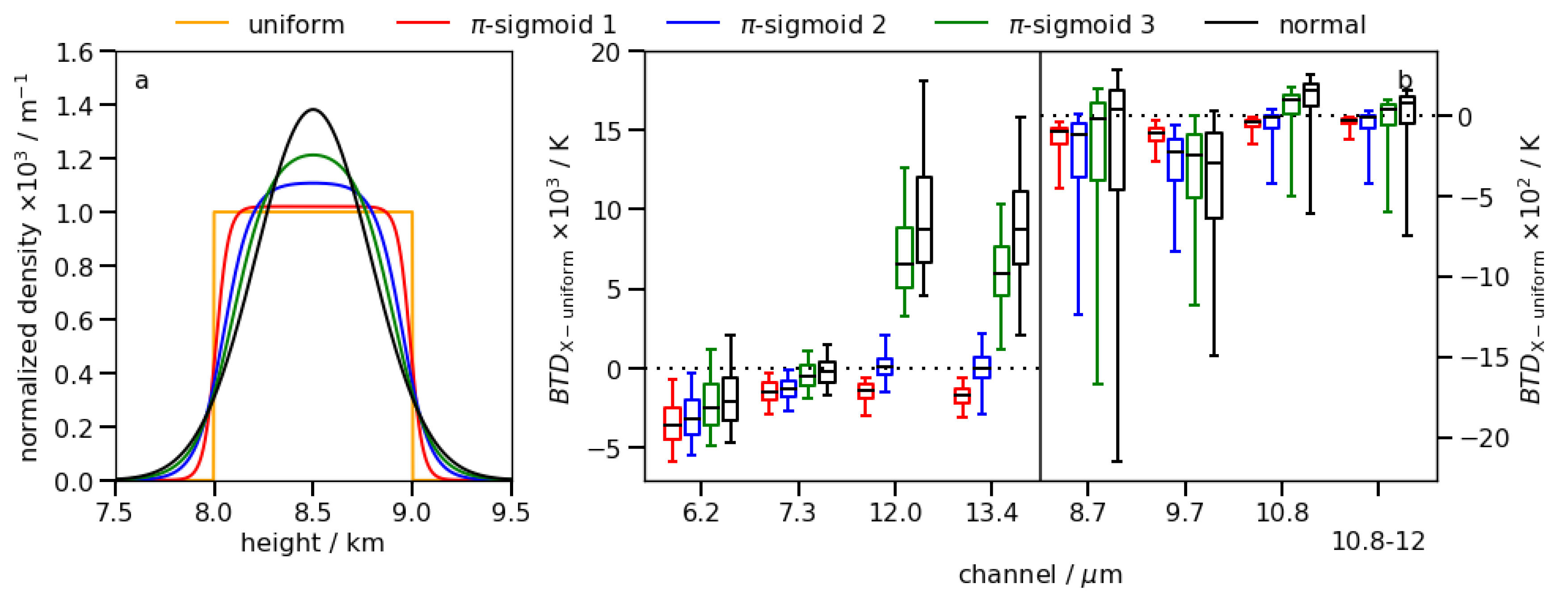
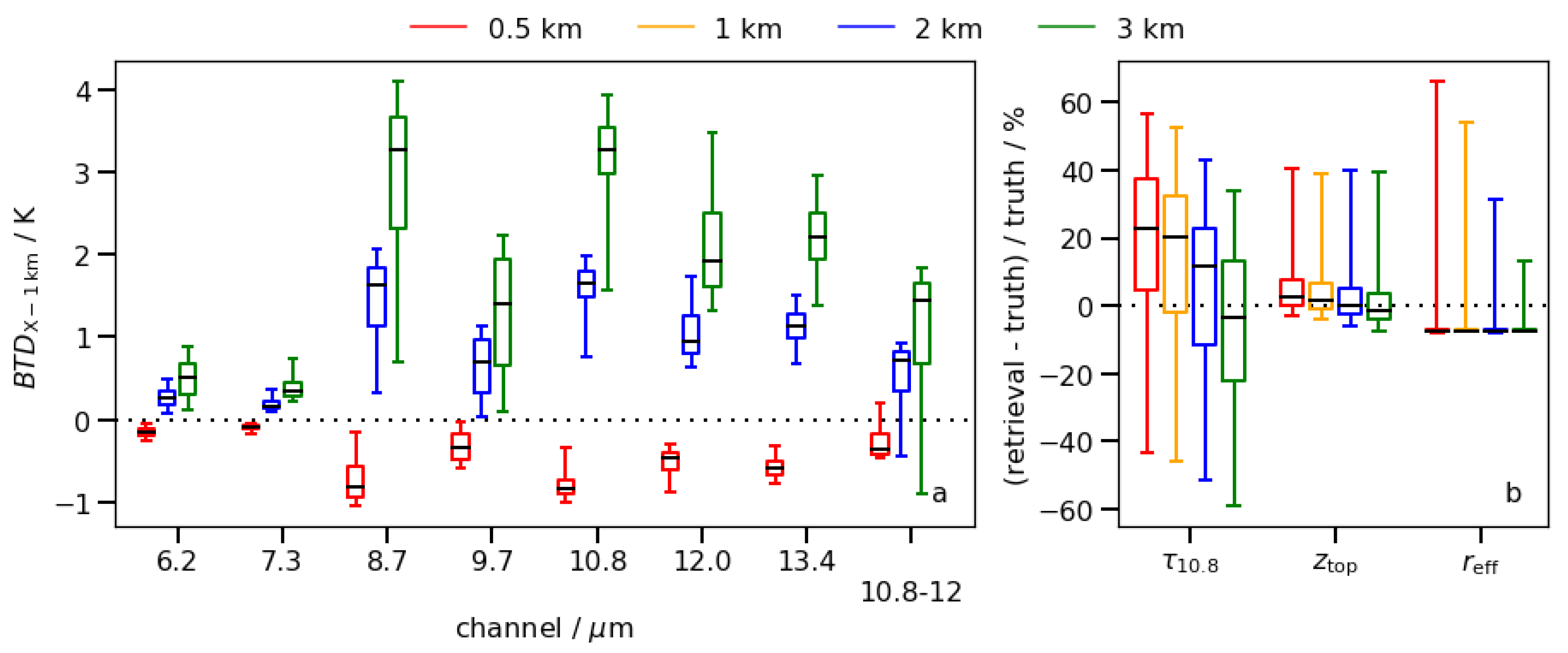
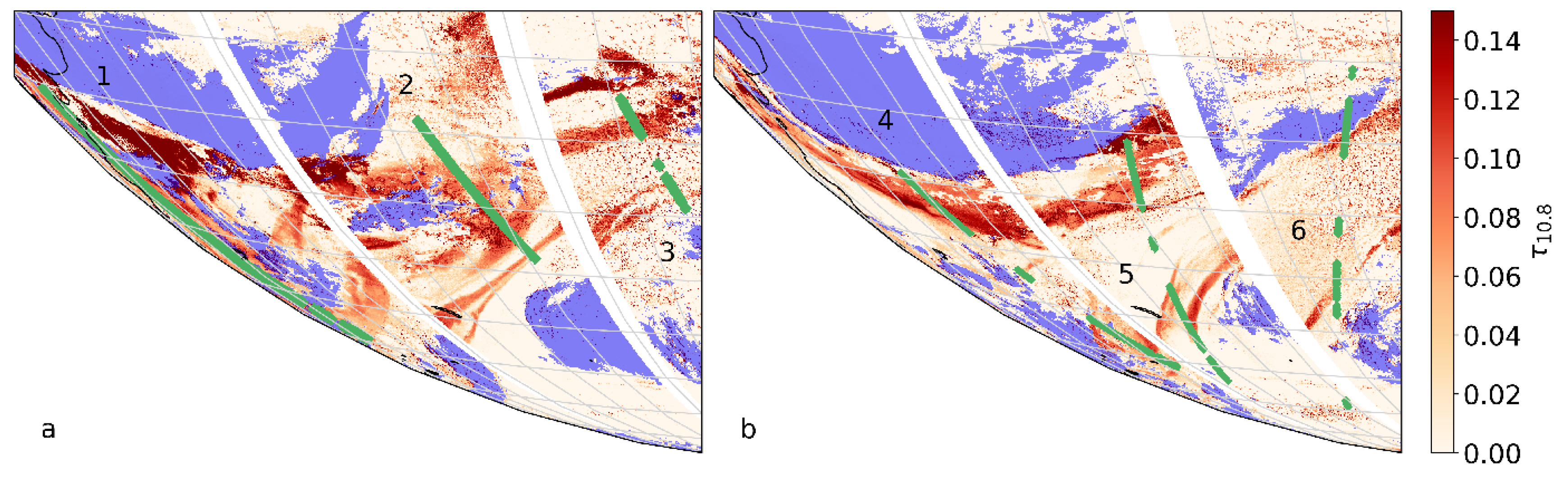
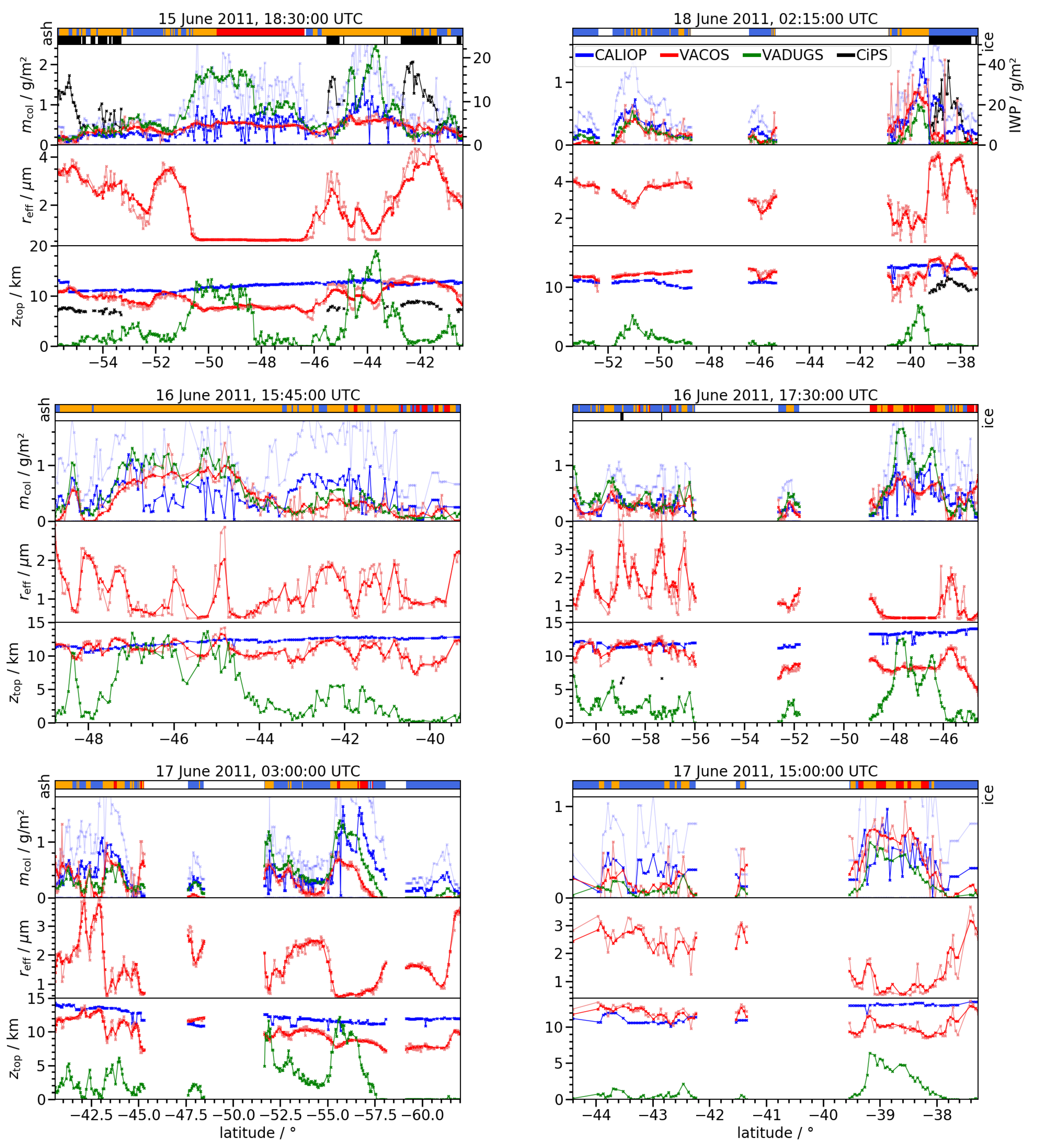
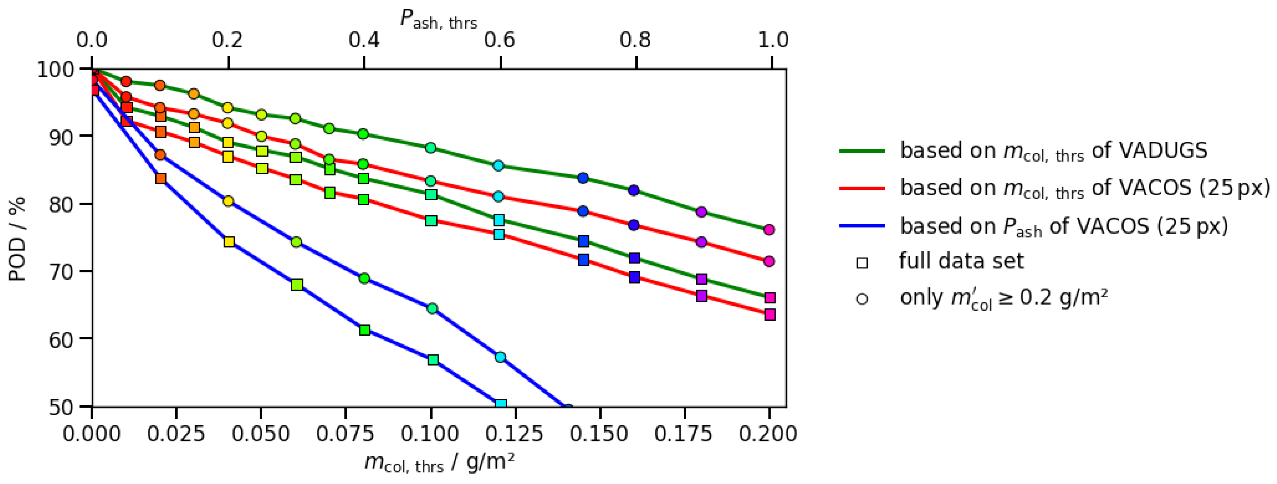
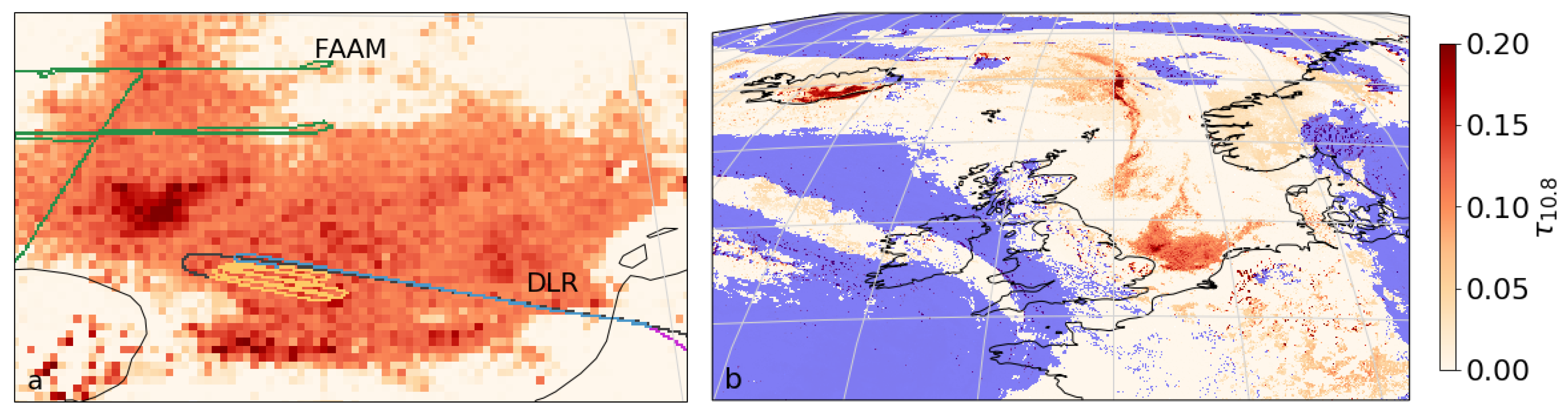
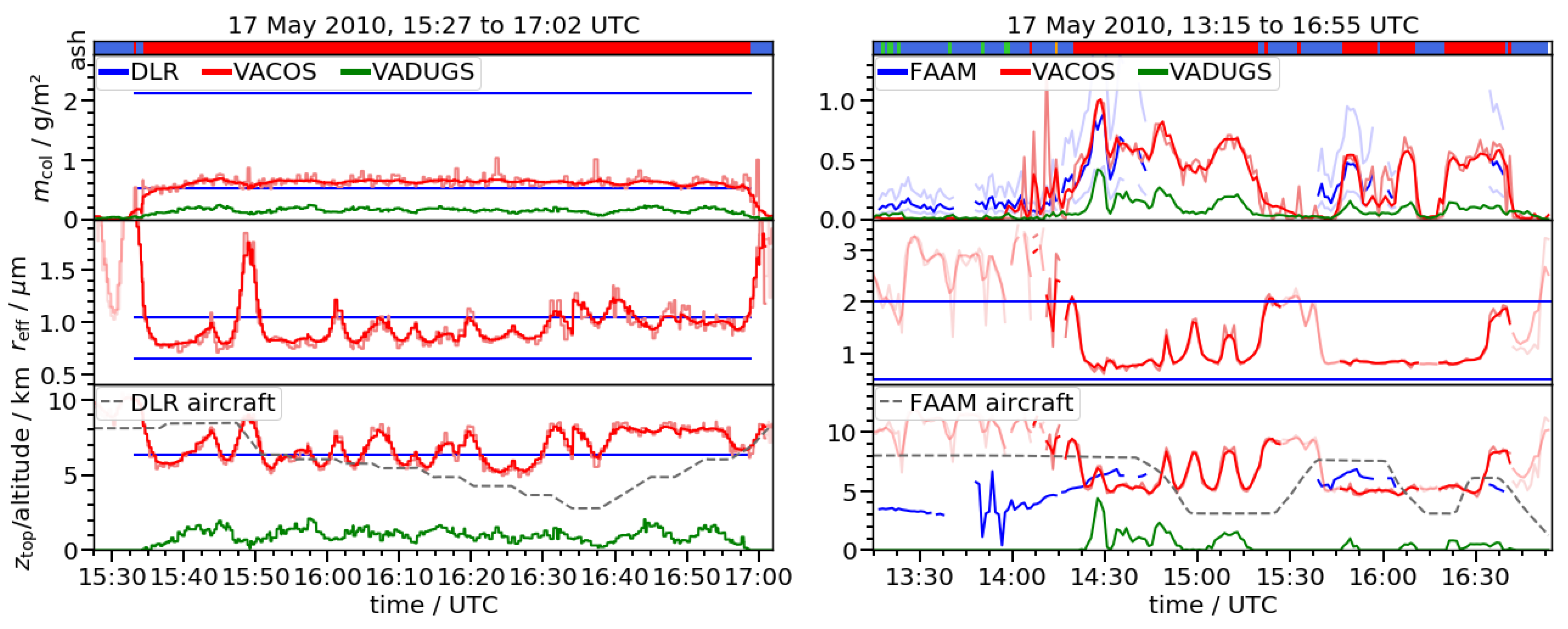

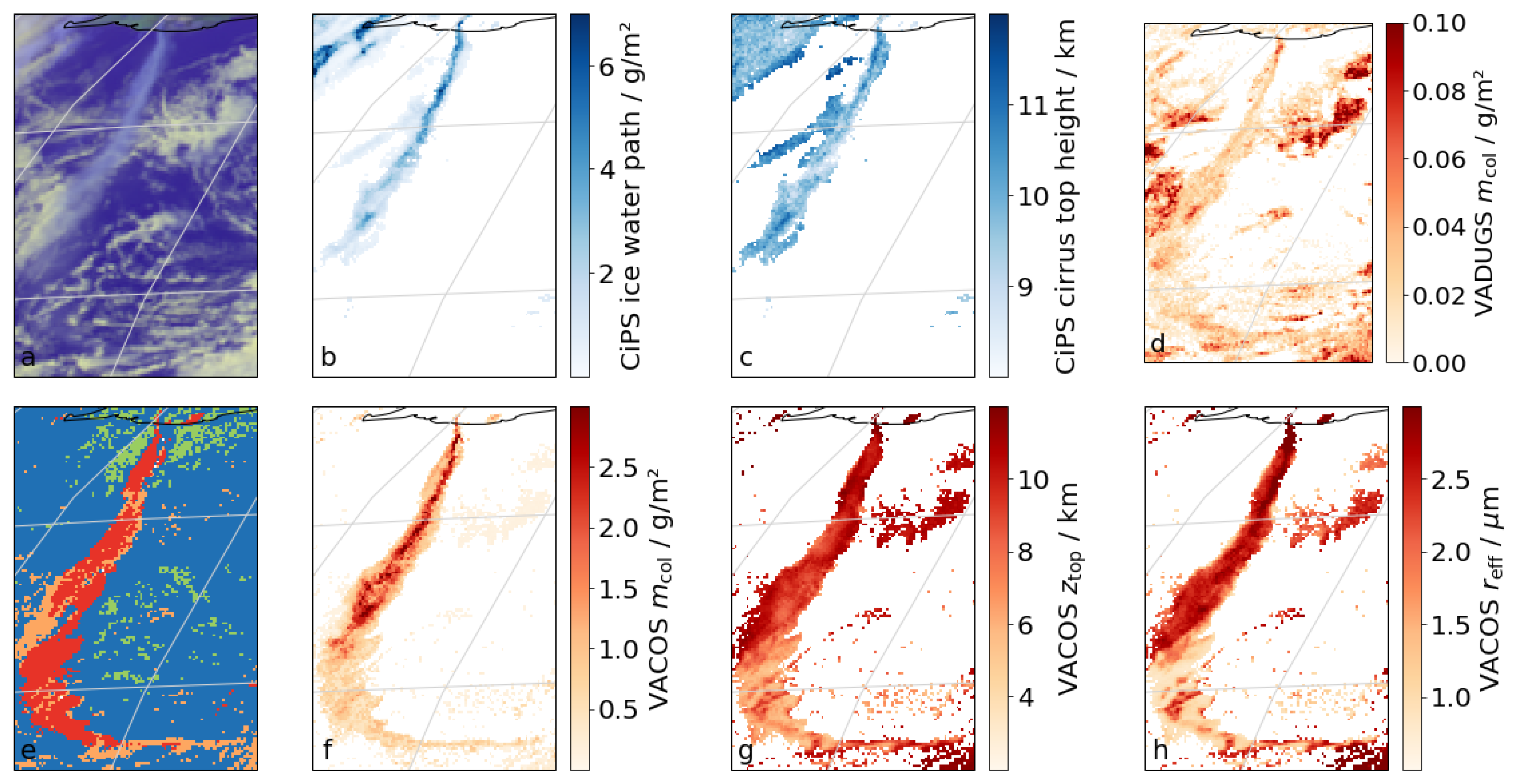
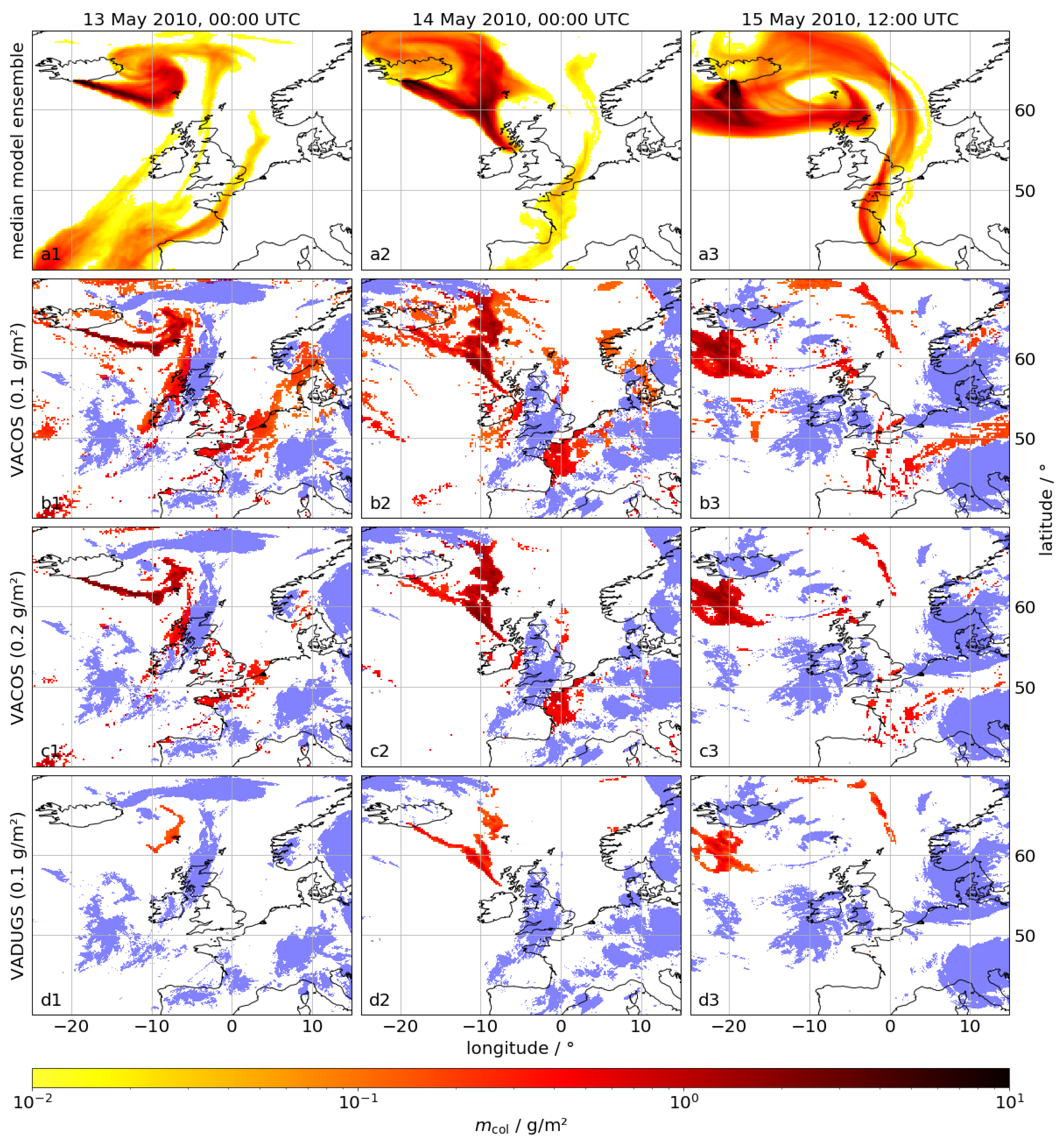
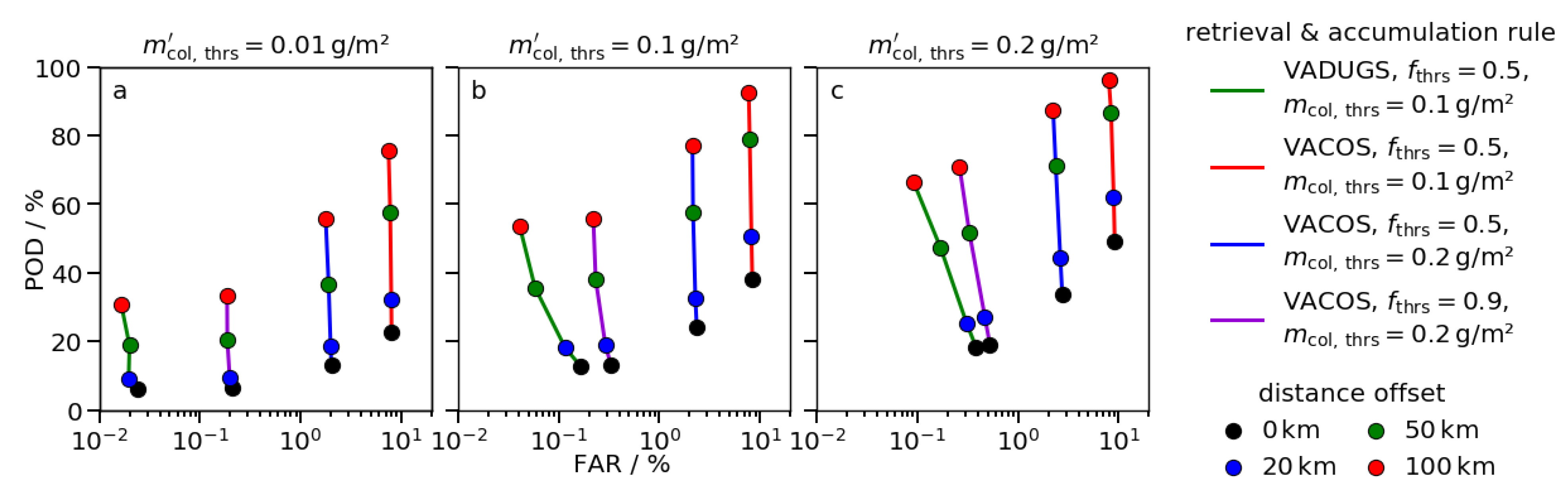
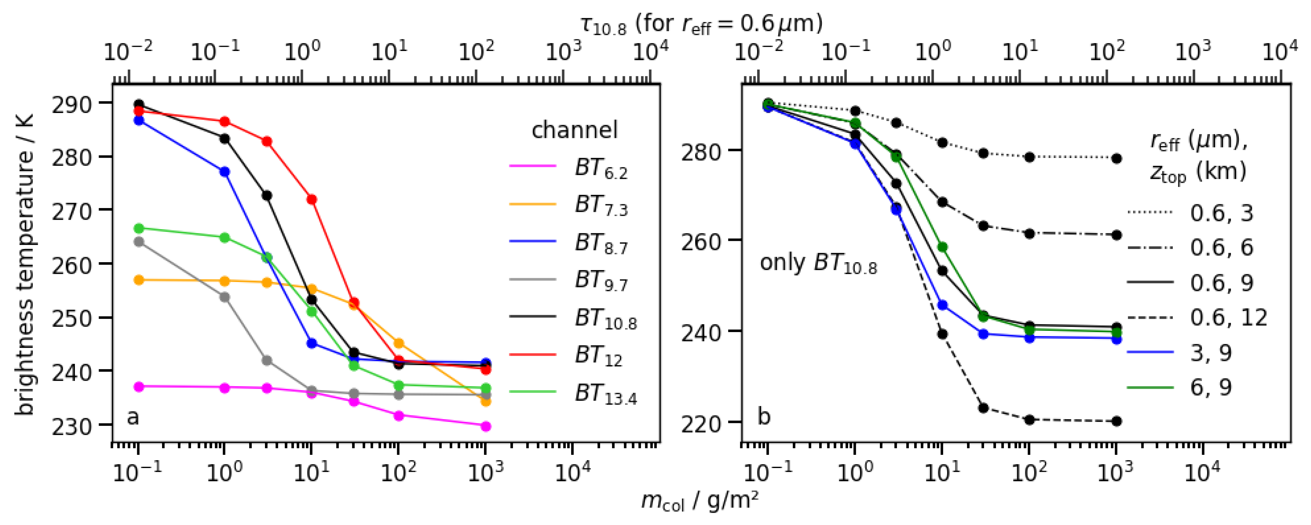
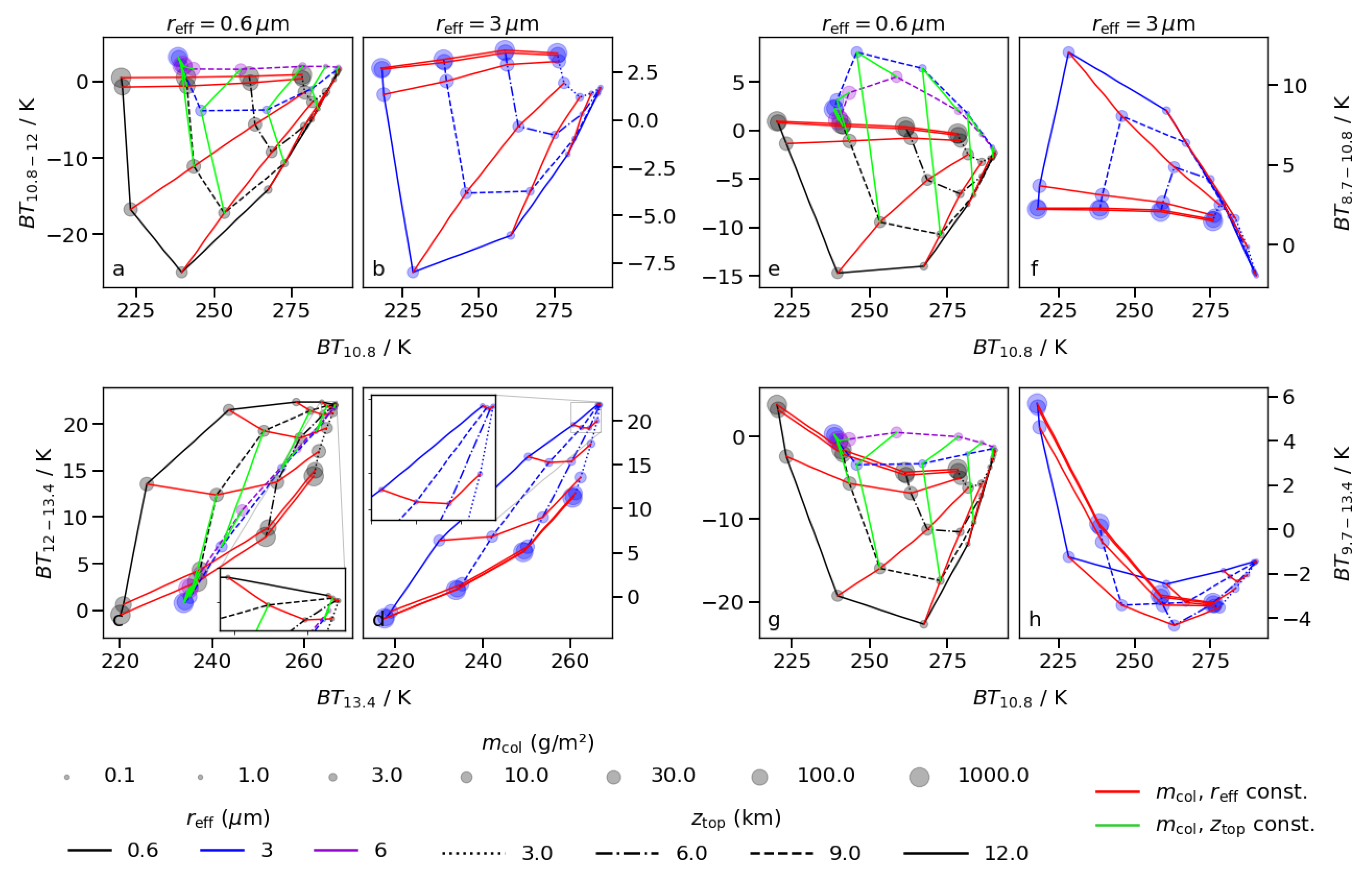
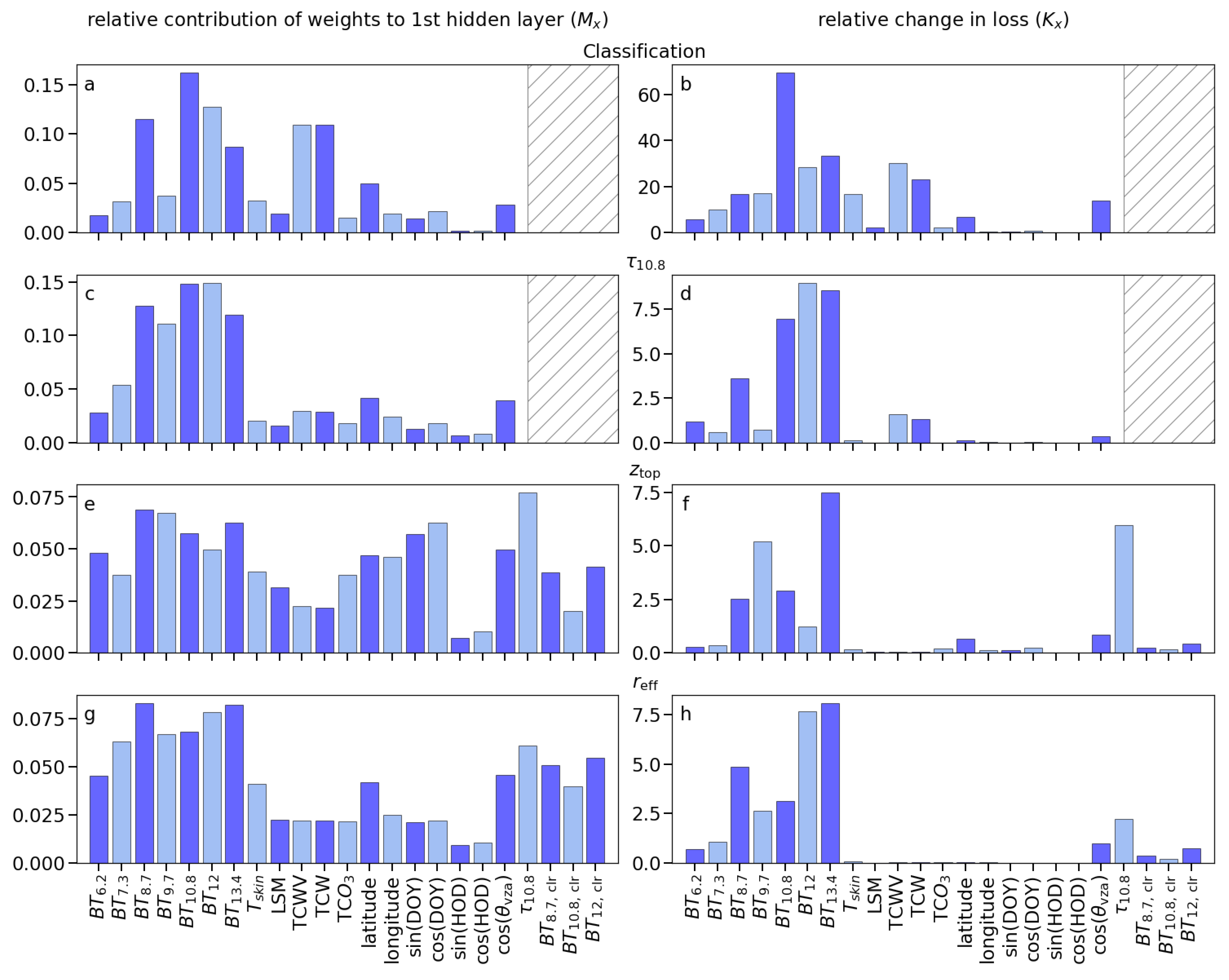
Publisher’s Note: MDPI stays neutral with regard to jurisdictional claims in published maps and institutional affiliations. |
© 2021 by the authors. Licensee MDPI, Basel, Switzerland. This article is an open access article distributed under the terms and conditions of the Creative Commons Attribution (CC BY) license (https://creativecommons.org/licenses/by/4.0/).