Abstract
Although soil moisture (SM) is an important constraint factor of evapotranspiration (ET), the majority of the satellite-driven ET models do not include SM observations, especially the SM at different depths, since its spatial and temporal distribution is difficult to obtain. Based on monthly three-layer SM data at a 0.25° spatial resolution determined from multi-sources, we updated the original Priestley Taylor–Jet Propulsion Laboratory (PT-JPL) algorithm to the Priestley Taylor–Soil Moisture Evapotranspiration (PT-SM ET) algorithm by incorporating SM control into soil evaporation (Es) and canopy transpiration (T). Both algorithms were evaluated using 17 eddy covariance towers across different biomes of China. The PT-SM ET model shows increased R2, NSE and reduced RMSE, Bias, with more improvements occurring in water-limited regions. SM incorporation into T enhanced ET estimates by increasing R2 and NSE by 4% and 18%, respectively, and RMSE and Bias were respectively reduced by 34% and 7 mm. Moreover, we applied the two ET algorithms to the whole of China and found larger increases in T and Es in the central, northeastern, and southern regions of China when using the PT-SM algorithm compared with the original algorithm. Additionally, the estimated mean annual ET increased from the northwest to the southeast. The SM constraint resulted in higher transpiration estimate and lower evaporation estimate. Es was greatest in the northwest arid region, interception was a large fraction in some rainforests, and T was dominant in most other regions. Further improvements in the estimation of ET components at high spatial and temporal resolution are likely to lead to a better understanding of the water movement through the soil–plant–atmosphere continuum.
1. Introduction
Understanding water and heat exchange information of the soil–plant–atmosphere continuum (SPAC) is imperative to better manage more restricted water resources in the future. As one of the most important connecting terms in SPAC [1], evapotranspiration (ET), which consists of evaporation from wet surfaces (E) and transpiration through plants (T), is critical for both the energy budget and water balance in the earth–atmospheric system. Normally, vegetation T is a physiological process that is closely associated with CO2 assimilation and has a great influence on the gross productivity of terrestrial ecosystems, while evaporation from wet canopy surfaces (Ei) or soil (Es) is often regarded as a wasteful loss of water and does not directly contribute to the ecosystem productivity [2,3]. Therefore, ET partitioning is of prime importance for the water resources and forests management and the agriculture practice. Over the past five decades, much effort has been devoted to the development of techniques and algorithms for ET or its components estimation, as documented by a substantial body of literatures [4,5,6,7]. However, estimates of ET or its components are still a major challenge for the complex climatic and underlying conditions.
In general, ET partitioning methods can be grouped into two categories: (1) Field measurements (i.e., micro-lysimeter, Bowen ratio, isotopes, sap flow, and the eddy covariance (EC) technique, etc.) [8,9,10,11,12,13] and (2) models such as remote sensing-based physical models, land surface models (i.e., the Shuttleworth–Wallace model, the energy and water balance model, the soil–water–energy and transpiration model, and the two-source energy balance model, etc.) [14,15,16,17,18]. Due to the difficulty of using relatively few scattered point measurements to infer regional variability [19], remote sensing-based ET models have become a dominant means for providing spatially distributed regional ET information on land surface, as they have greatly improved the large-scale observation of soil and vegetation dynamics [20]. Among the remote sensing-based ET models, the physical models, such as the Penman–Monteith (PM) ET algorithm and Priestley Taylor–Jet Propulsion Laboratory (PT-JPL) ET algorithm, focusing on the dynamics of the ET process, have been widely used [20,21,22,23,24]. Particularly, the PT-JPL algorithm, a simplified version of the more theoretical PM ET algorithm that avoids the computational complexities of aerodynamic resistance, has outperformed many ET models [17,25]. Although the PT-JPL ET algorithm utilizes eco-physiological and atmospheric constraints to regulate the potential ET flux to an actual ET flux, such as the other ET remote sensing algorithms, it also lacks soil moisture (SM) control.
SM can not only control the conversion of incident radiation into sensible and latent heat fluxes but also determine the distribution of rainfall in infiltration, runoff, and evaporation [26]. Up until now, only a few studies have been conducted to estimate ET components using SM observations, mainly since the accurate values of SM observation are difficult to obtain. Instead, previous studies usually use the land surface temperature and vegetation index, which can serve as proxy indicators of the surface moisture status over a range in spatial scales [27], to estimate plant T and Es [28,29]. Along with the constant development of remote sensing techniques on SM (e.g., the global Soil Moisture Climate Change Initiative project, SMCCI, 1978; Soil Moisture and Ocean Salinity, SMOS, 2009; Soil Moisture Active Passive, SMAP, 2015), SM data have become increasingly available in recent years [30,31]. Within this context, Purdy et al. (2018) incorporated the launch of the SMAP satellite-derived surface SM control on the PT-JPL ET algorithm to estimate Es and canopy T [24]. Walker et al. (2019) presented a modified ET model using a surface actual water vapor pressure parameter, which was estimated by incorporating the SM from SMAP products [32]. It is important to note that the SMAP mission was first launched in January 2015, and the length of SM observations is relatively short. Indeed, the increasing accuracy and a variety of spatial scales of SM datasets will provide much assistance in ET estimates. However, many of these remote sensing techniques can only provide SM estimates for the surface [27,33,34,35,36,37], which cannot satisfy the transpiration water requirements for the vegetation with deeper roots, such as trees and shrubs. Therefore, in order to investigate the SM effect on vegetation T estimation, effective SM data from the deeper sources should first be obtained.
Various adaptations of SM normalized by soil properties to compute the relative extractable water (REW) have been applied to limit Es or T [24,29], while SM under the canopy is just one of numerous environmental variables that constrains the photosynthesis and/or canopy evaporative demand [4,20,38,39]. Moreover, the estimation accuracy of vegetation T not only relies on the quality of environmental variables, such as temperature, vapor pressure, radiation, and SM data, but also relates to the plant types, canopy heights, and aboveground biomass [23,24,40]. However, the impact of environmental variables and plant and soil types on soil water availability is difficult to quantify and subject to much uncertainty. Recently, the availability of high-quality meteorological forcing datasets and observations of vegetation characteristics and canopy heights, as well as SM-observing satellites, together with data assimilation techniques, provides us the opportunity to gather further information on plant sensitivity to environmental conditions [24,32]. Nonetheless, accurate documentation of the spatial and temporal distribution of multi-layer SM and quantification of the effect of the environmental conditions on vegetation T are important in the ET and its components’ estimates.
Overall, to the best of our knowledge, there is a scarcity of studies incorporating SM of multi-layers into the physically and remote sensing-based ET algorithm, as well as of those focusing on the role of SM in different ET components estimates. The primary objective of this study is to estimate ET components at monthly scale based on a modified PT-JPL ET algorithm by incorporating the SM constraints. To this end, SM data of multi-layers are integrated from observation and remote sensing products. As a case study, both the original PT-JPL ET algorithm and the modified algorithm (here-after called PT-SM) are evaluated using the observed ET from 17 eddy covariance sites across different land covers in China. Ultimately, we also apply the new PT-SM model to the whole of China using SM data at different depths, and the individual component contribution to the mean annual ET is investigated.
2. Materials and Methods
2.1. PT-JPL Algorithm
Potential evapotranspiration (PET, in mm) is defined in terms of the radiation- and temperature-based Priestley–Taylor (PT) equilibrium equation:
where α is the PT coefficient of 1.26, ∆ is the slope of the saturated vapor pressure curve (kPa °C−1), γ is the psychrometric constant (~0.066 kPa °C−1), λ is the latent heat of vaporization (kPa °C−1), Rn is the net radiation at the surface (MJ m−2), and G is the ground heat flux (MJ m−2).
Subsequently, Fisher et al. (2008) developed a modified PT model (i.e., the PT-JPL model) to scale the PET down to the actual ET using eco-physiological constraints and soil evaporation partitioning, which are driven by atmospheric moisture (vapor pressure deficit and relative humidity, VPD and RH) and vegetation indices (normalized and soil adjusted vegetation indices, NDVIs, and the enhanced vegetation index, EVI) [37]. The PT-JPL algorithm estimate ET at the monthly scale is defined as follows:
where fwet is the relative surface wetness (RH4); fsm is a soil moisture constraint (, where is calculated by Tmax and ); fC is the green canopy fraction (fAPAR/fIPAR) with fAPAR being the fraction of absorbed photosynthetically active radiation (PAR) absorbed by green vegetation cover (m1EVI + b1) and fIPAR the fraction of intercepted PAR (m2NDVI + b2); fT is a plant temperature constraint (exp(−((Tmax − Topt)/Topt)2)); fM is a plant moisture constraint (the ratio between fAPAR and fAPARmax); Tmax is the maximum air temperature; and Topt is Tmax at max (RnTmaxEVI/VPD). is the net radiation at the soil surface calculated as:
where = 0.60, and LAI is the leaf area index; is the canopy net radiation ().
2.2. PT-SM Algorithm
In the PT-JPL model, the soil water deficit index, fsm () is employed to constrain the rate of evaporation from the soil surface according to the Bouchet’s complementary hypothesis that the surface moisture status is linked to the evaporative demand of the atmosphere [37]. In the original PT algorithm, the REW is usually used as an index that normalizes the impact based on the soil moisture and soil properties [41]. Note that Es is driven by moisture within the top few centimeters of the soil profile. Therefore, with the aid of observed surface soil moisture (SM, m3 m−3), the scalar fREW can be calculated from the following equation:
where SM1 is the 0–5 cm soil moisture (m3 m−3); SM1fc and SM1wp are the soil field capacity and soil moisture at the wilting point, respectively. Therefore, the new Es equation is conducted by replacing fsm with fREW:
In the original PT-JPL formulation, the plant moisture stress is inferred from the deviation from maximum greenness (), which is calculated by normalizing phenological parameters by the maximum observed value per pixel. Actually, at the monthly scale, the latent responses from vegetation to soil moisture deficits can also affect the vegetation T to some extent, especially for arid and semi-arid regions [23]. To evaluate the influences of plant access on atmospheric demand and of deeper water storage intensification or mitigating vegetation sensitivity on water availability, the transpiration response curve to soil water availability can be drawn (the relation between transpiration stress and soil moisture conforms to the exponential form), and the results indicate that higher canopy heights show less sensitivity to soil water availability [24,42]. Furthermore, the root system developed in different vegetations is different. Generally, the depth of root system is related to plant species, but it is also related to the climate [24]. For example, in the subtropical region, there is plenty of rain, tree species can get enough water from the surface soil, so they should not grow deeper into the soil. Therefore, in this study, vegetation is divided into four categories, forest, shrub, grass, and crop, and a new eco-physiological scalar is formulated as follows:
where SRHk is the soil relative humidity at k-layer. Three layers (0–5, 5–20, and 20–100 cm) are used in this study, k = 1, 2, 3 for frost and shrub covers, and k = 1, 2 for grass and crop covers. While the transpiration constraint is supposed to be related to the type and height of vegetation, and the climate condition, which can be calculated by:
where is the critical k-layer soil moisture at which soil water availability limits ET; = is a canopy height (CH) scalar set to range from 1 to 5, and the square root is formed from Martens et al. (2017) [40]; is a vegetation type (VT) scalar that represents the impact of vegetation sensitivity on soil water availability; and is a climate (CL) scalar, e.g., the deep-rooted tree species can gradually change into the shallow-rooted species in the subtropical environment. Both the vegetation type and climate scalars are set to 0–1, which are determined by comparing the modeled ET series to the observations.
Thus, the algorithm of vegetation transpiration can be described as follows:
2.3. Evaluation
Eddy covariance (EC) observations of latent heat flux (LE) across different land cover types are often used for ET model evaluation. The performances of PT-JPL and PT-SM algorithms for estimating monthly ET were evaluated by comparing the simulated monthly ET series against ET values observed by EC sites. Four statistics, namely the coefficient of determination (R2), the Nash–Sutcliffe Efficiency (NSE), the root mean square error (RMSE), and the amount of system deviation (Bias), were used to evaluate the performances of these two PT models. The four statistics are defined in the forms of
with as the average of the observed , where is the number of time-steps.
2.4. Eddy Covariance (EC) Flux Data
Ranging from 3.8 to 53.6°N and from 73.6 to 135.1°E (Figure 1), China is the third largest national territorial area in the world with a total area of over 9.73 million km2. With such a large area, China is characterized by a complex climate and diverse land cover types and soil types (Figure 1B,C). Ground-measured LE data of 17 eddy covariance sites from China FLUX, USCCC, WATER, and Asia flux, distributed in different land cover types of China, were collected to validate the PT-JPL and PT-SM algorithms (Figure 1A and Table 1). The land cover types of the flux towers include croplands (Crop; four sites), deciduous needle leaf forests (DNF; one site), evergreen broadleaf forests (EBF; two sites), open shrubland (OSH; one site), evergreen needle leaf forests (ENF; one site), grasslands (GRA; seven sites), and mixed forests (MF; one site). Our analysis is based on EC site data during the period of 2003–2011 (see Table 1). It has been noted that the sum of sensible heat (H) and LE as measured by the EC method is generally less than the available energy [43]. Therefore, the original ground-measured LE was corrected using the method put forward by Twine et al. (2000) and Jung et al. (2010) [19,44].
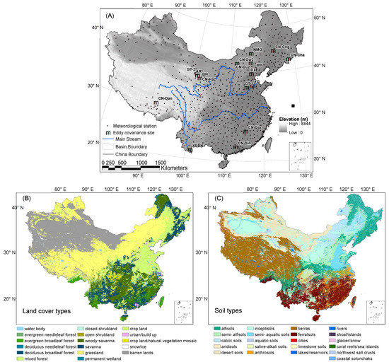
Figure 1.
(A) Locations of the study area, 17 eddy covariance sites and 577 meteorological stations. (B) Land cover classification and (C) soil classification from the International Geosphere–Biosphere Programme (IGBP) used in this study.

Table 1.
Description of 17 eddy covariance sites used in this study.
2.5. Observed Meteorological and Hydrological Data
A high spatial–temporal resolution (with a daily temporal resolution and a spatial resolution of 0.1°), gridded, near-surface meteorological dataset from the China Meteorological Forcing Dataset (CMFD) was used in this study. The dataset was made through fusion of remote sensing products, reanalysis of the dataset, and in situ observations at weather stations [45]. Monthly precipitation, relative humidity, radiation, and maximum and minimum temperatures at a spatial resolution of 0.25° during the 2003–2015 period were calculated and resampled.
2.6. Remote Sensing NDVI, EVI, and LAI Data
The time series of EVI and NDVI were acquired from moderate resolution imaging spectroradiometer (MODIS) products (MOD13A3), which provide 1 km spatial and monthly temporal resolutions. We used an average of four surrounding pixels around the EC flux sites to acquire the EVI and NDVI values. The LAI and FPAR products, potential factors influencing total ET segmentation, were extracted from MCD15A2H at 500 m spatial and 8-day temporal resolution. The 8-day temporal EVI, NDVI, LAI, and FPAR records were integrated into a monthly scale.
2.7. Canopy Height and Soil Moisture Data
Observations of canopy height were used to model plant sensitivity to water content at different depths. These canopy height (CH) and soil relative humidity (SRH) datasets of 376 agricultural gas stations spanning from 2003 to 2015 on the China meteorological data network (http://data.cma.cn (accessed on 11 June 2021)) were selected. Since the datasets only include the CH and SRH data of the cropland, the CH from the Geoscience Laser Altimeter System (GLAS) on the Ice, Cloud, and Land Elevation Satellite [46] and soil moisture obtained from the outputs of the GLDAS-2 Noah Land Surface Model (LSM) L4 model [47], which here-after is referred to as LDAS-derived SM, were employed to enrich the basic study data. Considering the different spatial–temporal resolution of each SM data product (see Table 2), in this study, using the multiple linear regression and trapezoidal method [48], monthly SM data from 2003 to 2015 of three layers (0–5, 5–20, and 20–100 cm) were reconstructed through integrating the observed precipitation, farmland SRH observation, SM dataset from Yang et al. (2020) [49], GRACE-derived ∆TWS [50], and GLDAS SM outputs at different depths (0–10, 10–40, and 40–100 cm).

Table 2.
Overview of the data used to reconstruct soil moisture in the study.
The multiple linear regression used in our study is in terms of
where SM is the soil moisture; SRH is the soil relative humidity, SRH = SM/SMfield moisture capacity 100%. During January 2002–December 2011, we define , then the coefficients ( and ) are estimated, and during January 2012–December 2015 are calculated. Note that the relationship between SRH observations and products was transplanted to the neighbored grid where there was a lack of observations.
The trapezoidal method [51] used in this study can be described as:
where the subscript of refers to the soil layer (from i = 1 to k); k corresponds to the final depth of measurement; and is the depth interval between two successive measurements.
3. Results
3.1. Spatial Distribution Characteristics of Soil Moisture
The estimation and prediction of SM, especially the root zone SM, have gained the interest of researchers [52,53]. Overall, many kinds of methods, including land surface modeling and the data assimilation technique, have been applied to estimate the multilayer SM. In this study, the monthly SM data from 2003 to 2015 of three layers (0–5, 5–20, and 20–100 cm) were reconstructed from multi-sources. Particularly, SM data collected at three observational networks (i.e., Ngari, Maqu, and Naqu; detailed information can be found in Yang et al. (2020)) across the Tibetan Plateau were employed to validate the reconstructed SM dataset [49]. Due to the lack of observation from deeper soils, Figure 2 only shows the comparison of the LDAS-derived and reconstructed monthly SM with the observed ones in the three layers of Naqu and surface layer of Ngari and Maqu. Both the observed station-averaged SM and its standard deviation are given in this figure. Only the LDAS-derived SM at a depth of 5 cm in the Ngari network is higher than the in situ data, as the LDAS-derived SM in the Maqu and Naqu networks are lower than the in situ data. This phenomenon might be due to the fact that the LDAS-derived SM only denoted liquid water and did not account for soil ice. In general, the reconstructed SM is much closer to the observation in all three networks. However, the Ngari network still exhibits underestimation in summer (Figure 2A), and the Naqu network exhibits a minor amount of overestimation in summer (Figure 2C).
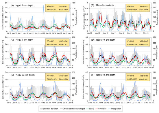
Figure 2.
Temporal variability of observed station-averaged soil moisture and its standard deviation, LDAS–derived soil moisture, and reconstructed soil moisture at (A) 5–cm depth in the Ngari network; (B) 5–cm depth in the Maqu network; (C) 5–cm depth in the Naqu network; (D) 10–cm depth in the Naqu network; (E) 20–cm depth in the Naqu network; (F) 40–cm depth in the Naqu network.
Spatial distributions of the reconstructed SM of 0–5, 5–20, and 20–100 cm averaged over 2003–2015 are respectively plotted in Figure 3. For all depths, the SM values range from 0.007 to 0.600, with the high values (over 0.4) distributed in northeast China and the southern part of China. In contrast, the SM values are relatively small in northwest China, the upper and middle reaches of the Yellow River, and western part of the Tibetan Plateau. From Figure 3A–C, we can also see that the SM values of individual depth are different, for example, the SM values of 0–5 cm in depth in southwest China are higher than those of 5–20 and 20–100 cm in depth. This region belongs to the tropical rainforest climate, the forest coverage is high, and the surface layer of soil has a strong capacity of water fixation [54]. A significant positive correlation between SM and P in eastern China has been identified in many previous studies [55,56]. Despite this, the relation between SM and P is a complex non-local process, and it is still unclear whether it represents the discovery of relevant phenomena or the explanation of the possible mechanism.

Figure 3.
Spatial distribution of the reconstructed (A) 0–5 cm, (B) 5–20 cm, and (C) 20–100 cm soil moisture, respectively averaged over 2003–2015.
3.2. Comparison of Algorithm Parameters
The differences between the parameters of the PT-JPL algorithm and PT-SM algorithm lie in the core of the performances of these two algorithms. Therefore, before we evaluate the performances of the PT-JPL algorithm and PT-SM algorithm at EC sites and hydrological catchments, the model parameters, including soil moisture constraint on soil evaporation fsm, fREW, soil water availability constraint on transpiration fM, and fTRM are firstly examined and compared. As a typical site with different underlying surfaces, Figure 4 shows the variation plot between fsm and fREW, fM and fTRM calculated from the reconstructed SM data at the CN-Qia (forest) flux tower, CN-Ha2 (shrub) flux tower, CN-Du2 (grass) flux tower, and YC (crop) flux tower. It can be seen that for all biomes, almost all of the fTRM values are larger than the fM values, and the values of fREW are larger than those of fsm, especially in the valley values. Comparatively, the values of fREW are much larger than those of fsm for the forest and the shrub biomes, while those of fTRM are much larger than those of fM for the forest and the crop land cover types. This result is reasonable, as several studies have shown that in comparison with shorter vegetation, taller vegetation is less sensitive to soil water deficits since the deeper root can absorb water from deep soil or groundwater, where there is a delay in response to drought [23,57]. For instance, Figure 4G,H indicates that for the crop biome, the fREW series closely follows fsm, while in the peak values, the values of fREW are larger than those of fsm. For fTRM, it can also be clearly seen that the new soil water availability constraints on transpiration are always higher than the original fM, especially at the fM valley values (mostly occurring in the period from October to next March). Moreover, fTRM being considerably higher could be due to the fact that Yucheng tower is an agricultural experiment station that monitors areas in which wheat and corn crops are mainly planted in winter and summer, respectively.
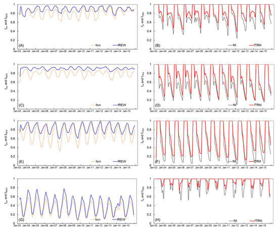
Figure 4.
Comparisons of smoothed fsm and relative extractable water (fREW), fM and new soil water availability constraint on transpiration (fTRM) during 2003.1–2015.12 at (A,B) CN–Qia (forest) flux tower, (C,D) CN–Ha2 (shrub) flux tower, (E,F) CN–Du2 (grass) flux tower, and (G,H) YC (crop) flux tower.
3.3. Comparison of Incorporating Soil Moisture into Soil Evaporation and Transpiration
Since the algorithm models individual ET components, we can separately quantify the added value from incorporating SM into soil E and canopy T. Consequently, we evaluated the updated PT-SM algorithm with SM incorporation into soil E (PT_Es), the updated algorithm with SM incorporation into T (PT_T), and the updated algorithm with SM incorporation into both soil E and T (PT-SM) compared with the original PT-JPL model. Comparisons among the four EC sites, i.e., CN-Qia (forest) flux tower, CN-Ha2 (shrub) flux tower, CN-Du2 (grass) flux tower, and YC (crop) flux tower, are shown in Figure 5. It can be clearly seen that incorporating explicit SM can improve estimates of monthly ET series. Especially at the Yucheng EC site, the updated PT-SM algorithm shows greater R2 and NSE (PT-JPL: 0.93 and 0.85; PT_Es: 0.95 and 0.91; PT_T: 0.91 and 0.98; PT-SM: 0.98 and 0.98, respectively), lower RMSE and Bias (PT-JPL: 11.29 and −8.09; PT_Es: 9.50 and −6.01; PT_T: 5.20 and −1.07; PT-SM: 5.02 and 1.17, respectively), and larger slopes (PT_Es: 0.840, PT_T: 0.941, PT-SM: 0.970) closer to 1.0 when compared with the PT-JPL model (PT-JPL: 0.821) (Figure 5D and Table 3). At the Yucheng EC site, by only replacing soil evaporation Es, R2 and NSE increased by 2% and 7%, respectively, and RMSE and Bias decreased by 16% and 2 mm, respectively. By only replacing canopy T, R2 and NSE increased by 4% and 15%, respectively, and RMSE and Bias decreased by 54% and 7 mm, respectively. According to our results, the performance of the updated PT-SM algorithm with SM incorporation into both Es and canopy T considerably improved (i.e., R2 and NSE increased by 5% and 15%, respectively, and RMSE and Bias decreased by 56% and 9 mm, respectively; Table 3) when compared with the original PT-JPL-modelled ET. Moreover, observations between 60 and 120 mm are better represented by the updated model with a scatter closer to the 1:1 line from raised underestimation in ET (see Figure 5).
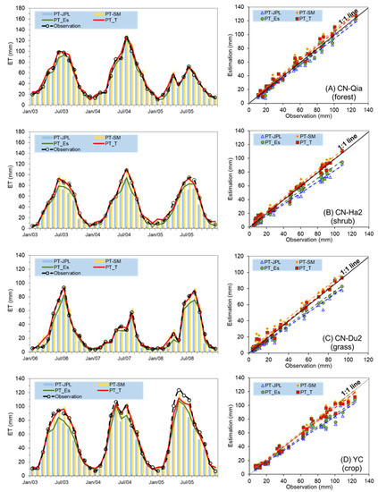
Figure 5.
Comparisons of monthly evapotranspiration (ET) from observation, original PT–JPL algorithm (PT–JPL), updated algorithm with soil moisture incorporation into soil evaporation (PT_Es), updated algorithm with soil moisture incorporation into transpiration (PT_T), and updated PT-SM algorithm; and scatter plot of ET model without and with soil moisture incorporation into the updated algorithm at (A) CN–Qia (forest) flux tower, (B) CN–Ha2 (shrub) flux tower, (C) CN–Du2 (grass) flux tower, and (D) YC (crop) flux tower.

Table 3.
Quantitative measures of original PT-JPL model, updated algorithm PT-SM with soil moisture incorporation into soil evaporation (PT_Es), updated algorithm with soil moisture incorporation into transpiration (PT_T), and updated PT-SM ET performance at monthly time-steps for 17 flux sites.
Among all of the EC towers, we noted that, by only replacing soil evaporation Es, the R2 and NSE increased by 2% and 7%, respectively, and the RMSE and Bias decreased by 20% and 3 mm, respectively. By only replacing canopy T, R2 and NSE increased by 4% and 18%, respectively, and RMSE and Bias decreased by 34% and 7 mm, respectively (see Table 3). The improvement to the updated PT-SM algorithm is more obvious at the EC towers in the arid area (PET/P > 1.7) than that at the EC towers in the humid regions (PET/P < 1.7), with the R2 and NSE being increased by 8% and 25%, respectively, and RMSE and Bias being decreased by 40% and 9 mm, respectively. In addition, both Figure 5 and Table 3 show that this improvement is strongly dependent on the simulation accuracy of vegetation T; the result also confirms that our approach of incorporating the soil moisture constraints into a simple algorithm can provide good estimates of ET series at different land cover regions.
3.4. Model Evaluation with In Situ Forcing
Both the PT-JPL and PT-SM algorithms were executed for in situ evaluation. The in situ modeled ET from both the PT-JPL and PT-SM show good consistency with the observations (Figure 6, Table 3). We noted a site-wide average improvement in R2, NSE, RMSE, and absolute Bias as a result of the model improvements. Sites are ordered from wet to dry (left to right; top to bottom) based on the aridity index (PET/P). The PT-SM algorithm demonstrates greater performance than that of the original PT model at water-limited sites (Table 3). On average, the PT-SM algorithm shows an apparent decrease in RMSE and absolute Bias (36% and 8 mm, respectively), a weak increase in R2 (5%), and a large increase in NSE (20%) when compared with the original PT-JPL model. An interesting feature is that the more overall statistical improvements are observed at CN-Cng and YC sites, two sites that both have relatively dry conditions (PET/P = 2.38 and 1.82, respectively; Figure 6M,I) and a large fraction of ET comes from soil evaporation. It can also be seen that at YC, AR, and CN-Cng sites, the PT-SM model demonstrates considerable improvements to the model estimation of ET during the seasonal dry term (Figure 6).
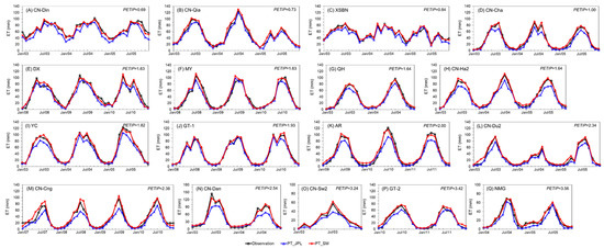
Figure 6.
In situ model performance across 17 eddy covariance sites ((A): CN–Din; (B): CN–Qia; (C): XSBN; (D): CN–Cha; (E): DX; (F): MY; (G): QH; (H): CN–Ha2; (I): YC; (J): GT–1; (K): AR; (L): CN–Du2; (M): CN–Cng; (N): CN–Dan; (O): CN–Sw2; (P): GT–2; (Q): NMG) distributed across China.
Compared with the observed 17 EC sites’ monthly ET series, the R2 and NSE of the PT-JPL monthly ET series are 0.94 and 0.90, respectively, and the RMSE and Bias are 10.05 and −6.34, respectively (Figure 7A). The R2 and NSE of the PT-SM monthly ET series are 0.97 and 0.96, respectively, and the RMSE and Bias are 5.90 and 2.13, respectively, when compared with the observed ET (Figure 7B). Among all of the land covers (biomes), both models represent the observed monthly ET series well, especially at the EC sites across the MF and Crop biomes. Only at the EC sites in the GRA land cover type, the two models represent the observed monthly ET series not so well. Comparing Figure 7B to Figure 7A, we can see that the PT-SM model provides much better improvements than those of the original PT-JPL model at the EC sites across the EBF and GRA land cover types. This phenomenon illustrates that at the EBF and GRA land cover regions, the PT ET model, considering the soil water availability constraint on transpiration, is better at reflecting the monthly ET series.
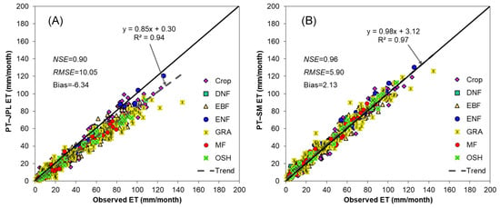
Figure 7.
Observed evapotranspiration (ET) at eddy covariance sites vs. (A) PT–JPL ET and (B) PT–SM ET. The solid line is the 1:1 line and the short dashed line is the trend line for ET series of all land cover types of the 17 EC sites.
3.5. Evapotranspiration Partitioning
As an important component of ET, the interception evaporation (Ei) of vegetation plays a vital role in water resources at both global and regional scales [23,57,58]. The ratios of canopy interception evaporation-to-precipitation (Ei/P) values of different land covers are notably different, with the averages for all biomes ranging from 0.11 to 0.27, but all values are below 0.30 (Figure 8 and Table 4). The average Ei/P for the ENF land cover is higher than that of other types, and the OSH biome has the lowest value (0.11). This may be related to different raining conditions and LAIs across land cover types. The Ei/P variation in the Crop biome is larger than that of other biomes, with values ranging from 0.11 to 0.27 and an average across the four Crop sites of 0.18. Research on the Ei/P ratio has attracted much attention. Under Mediterranean climate conditions, Llorens and Domingo (2007) discovered that for an annual rainfall of 90–800 mm, the mean relative interception was approximately 18% for trees and 31.6% for shrubs [59]. Miralles et al. (2010) reviewed 42 studies from different periods and found average Ei/P values for the EBF biome of 0.17 with ranges from 0.08 to 0.29, and the ENF biome average was 0.23 with ranges from 0.16 to 0.42 [57]. Gu et al. (2018) obtained the Ei/P from 11 terrestrial biomes based on 75 eddy covariance towers and found average Ei/P values for the Crop biome of 0.12 with ranges from 0.06 to 0.16, and the GRA biome average was 0.13 with ranges from 0.02 to 0.17 [58]. Compared with these previous studies, the overall variation is relatively consistent, but the Ei/P of the individual biome is somewhat different, which is most likely due to the fact that the EC sites used in this study are relatively few in number (e.g., Crop: 11 sites in Gu et al. (2018) vs. four sites in our study; GRA: 12 sites in Gu et al. (2018) vs. seven sites in our study) [58]. Overall, we found that the Ei/P variation in the land covers was large, ranging from 0.11 to 0.27, with an average of 0.16 among 17 sites (see Figure 8A), which is relatively reasonable compared with those of other similar studies (shown in Table 4). The canopy interception evaporation-to-evapotranspiration (Ei/ET) ratios across different land cover types are shown in Figure 8B. The average Ei/ET values across biomes range from 0.11 (OSH biome) to 0.32 (GRA biome). Large variations are noted within each land cover type, with the GRA biome having the greatest range (0.19–0.32) followed by the EBF biome (ranges of 0.20–0.28, respectively).
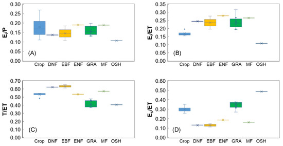
Figure 8.
Ratio of (A) canopy interception evaporation to precipitation (Ei/P) varies across different land covers; (B) canopy evaporation to total evapotranspiration (Ei/ET); (C) vegetation transpiration to total evapotranspiration (T/ET); and (D) soil evaporation to total evapotranspiration (Es/ET). Boxes mark the 75th and 25th percentiles and the solid lines and crosses in the boxes refer to the average and median values, respectively.

Table 4.
Annual ratios (average) of canopy evaporation losses to the total precipitation based on land cover types.
Figure 8C demonstrates that the average T/ET values across biomes range from 0.37 (GRA biome) to 0.65 (EBF biome). Large variations are noted within the GRA biome (ranges of 0.37–0.48). The average T/ET values for the Crop biome of 0.53 range from 0.49 to 0.55, and the EBF biome average of 0.63 has a range from 0.61 to 0.65 (Figure 9C). Overall, our estimated T/ET values are much lower than the 0.80–0.90 global values that Jasechko et al. (2013) found using isotope approaches, but similar with the results of Gu et al. (2018) [58,60], that used 75 eddy covariance towers across a wide range of biomes. Previous studies [6,13,16] also indicate that a large variability occurs in T/ET, which is partly due to different ET measurements, model structures, and inconsistent spatial and temporal resolutions of forcing data.
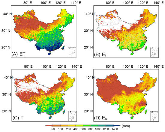
Figure 9.
(A) Mean annual PT–SM evapotranspiration (ET); (B) canopy interception evaporation (Ei); (C) vegetation transpiration (T); and (D) soil evaporation (Es) of multiyear (2003–2015) in China.
The soil evaporation-to-evapotranspiration ratios across different biomes are shown in Figure 8D. The average Es/ET values across biomes range from 0.11 (EBF biome) to 0.49 (OSH biome). The largest variation was noted for the GRA biome, having a greatest range of 0.27–0.39, followed by the Crop biome (range of 0.26–0.35). Our estimated Es/ET values are within the range of previously reported values.
3.6. Spatial Distributions of Mean Annual Evapotranspiration and Its Components
We applied the verified PT-SM algorithm to the whole of China for the period of 2003–2015 at a spatial resolution of 0.25° using CMFD meteorological data, MODIS products, and integrated SM datasets as described in Section 3.2, Section 3.3 and Section 3.4. Figure 9 shows the maps of mean annual ET, Ei, T, and Es over the period of 2003–2015. The mean annual ET distribution presented an intricate spatial structure with relatively high ET values in the southern China and low values located in the northwest. In most regions of the Xinjiang, Tibet, Qinghai, and Inner Mongolia provinces, the ET values are lower than 200 mm/year. In contrast, in the south of the Yangtze River and the Huai River, the ET values are higher than 800 mm/year. Generally, the mean annual ET increased from the northwest to the southeast (Figure 9A). Almost all of the Ei values in Xinjiang, Qinghai, and Inner Mongolia provinces are lower than 50 mm/year, especially in the northwestern part of China (barren lands) (Figure 9B). Similarly, T values of the northwestern part are lower than 100 mm/year, while only in the upper of Huai River basin, the Pearl River basin, central China, the southwest and southeast parts of China are the values of T higher than 600 mm/year. Notably, in the south region of Yunnan province, the T values are larger than 800 mm/year (Figure 9C). Furthermore, Es values lower than 100 mm/year were found in the arid and desert regions of the northwest part of China, while in some parts of southern China, the Es values are higher than 400 mm/year (see Figure 9D).
4. Discussion
4.1. Soil Water Availability Constraint on Evaporation and Transpiration
Many previous studies have tried to estimate soil moisture by measurements, such as time domain reflectometry soil moisture probes [61], hydrologic models [62], remote sensing techniques [63] or statistical learning tools such as support vector machines [64]. Unfortunately, most of these studies only paid attention to the SM at the surface. For vegetation with deeper roots, the transpiration water requirements also need the SM at the root zone. However, although the estimation of SM at the root zone has drawn great attention [53,65], its retrieval is difficult for spatial heterogeneity. Consequently, in this study, the multiple linear regression model and trapezoidal method were employed to estimate the SM of both the surface and root zone. The simulated SM performs the observation well (see Figure 2), and it was noted that the observation-driven model SM displays superior strength with coupling precipitation, soil relative humidity, ∆TWS, and GLDAS soil moisture outputs. These results further confirmed that for most regions, SM is closely related to precipitation and terrestrial water storage change, which is consistent with the findings of previous studies [34,53,65].
The performances of the updated PT-SM algorithm with the SM constraint separately on Es and T are different (see Table 3). Overall, it was observed that the updated PT-SM algorithm with the SM constraint on T (PT_T) performs the observation better than the PT-SM algorithm with the SM constraint on Es (PT_ Es), and the PT-SM model showed increased R2 and NSE and reduced RMSE and Bias, with the greatest improvements occurring in water-limited regions. With the aid of SMAP-derived surface soil moisture data, Purdy et al. (2018) indicated that the performance of the updated PT-SM algorithm with the soil moisture constraint on Es has improved performance on T across the 14 Ameriflux EC sites distributed across the US [24]. This result is different with our study, a difference that may have resulted from the difference in and estimates. In particular, some studies also demonstrated that SMAP might underestimate SM for the low biases in the Global Modeling and Assimilation Office surface temperature [39]. While Purdy et al. (2018) estimated the ET components with SMAP-derived soil moisture at a single depth (5 cm), in our study, SM data of three layers (0–5, 5–20, and 20–100 cm) were employed to estimate the ET components, which is a possible explanation of the difference.
Figure 10 is plotted to investigate the spatial difference of Es and T estimation by the PT-JPL algorithm and PT-SM algorithm. In contrast to the T estimated in July 2003 by the PT-JPL algorithm (Figure 10A), the estimated T results of the PT-SM algorithm showed higher values, especially in the central, southern, and northeastern parts of China (see Figure 10B), regions showing higher SM values (see Figure 3) and LAIs [66]. For Es estimation, the large differences also occurred in the northeastern, southern, and central parts of China (Figure 10C,D). The results further illustrate that estimation of ET components can only be improved by adequate soil moisture.
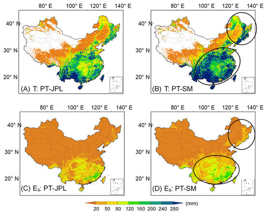
Figure 10.
Comparisons of vegetation transpiration (T) from the original PT–JPL algorithm (PT–JPL) (A) and updated PT–SM algorithm (B); comparisons of soil evaporation (Es) from the PT–JPL model (C) and PT–SM model (D) in July, 2003 across China.
4.2. Contribution of Each ET Component to the Total ET
We also evaluated the contribution of each ET component to the total ET by different algorithms for the whole of China. Figure 11 shows that the PT-SM algorithm considering SM estimated a higher T/ET value than those of the original PT-JPL model (64.9% vs. 53.7%) and lower Ei/ET and Es/ET values (21.2% vs. 15.4%; 25.1% vs. 19.7%). Overall, the average estimates of the T/ET value in our study are somewhat lower than previous studies’ results, although the T/ET value was improved by incorporating SM of multilayers into the original PT-JPL model. In essence, there are two possible reasons behind this phenomenon: (1) In terms of the site scale, Ei of vegetation has rarely been separately considered by previous studies, as usually, only Es and T are observed, and, therefore, the T/ET estimates would be higher; (2) different research scales, monitoring techniques or algorithms may also contribute to the variability—for instance, the isotope-based approach constrained by hydrologic decoupling always overestimates T/ET [60]. Additionally, the PT-SM Es/ET and Ei/ET values of our study are larger than the similarly reported fractions from the GLEAM model by 7–15% and 11–12%, respectively [23,57], but similar with Es/ET, T/ET, and Ei/ET at 23 ± 1.7%, 54 ± 1.6%, and 21 ± 0.8% of total ET, respectively, as reported in Purdy et al. (2018). It is worth noting that all of these studies focus on the global scale.
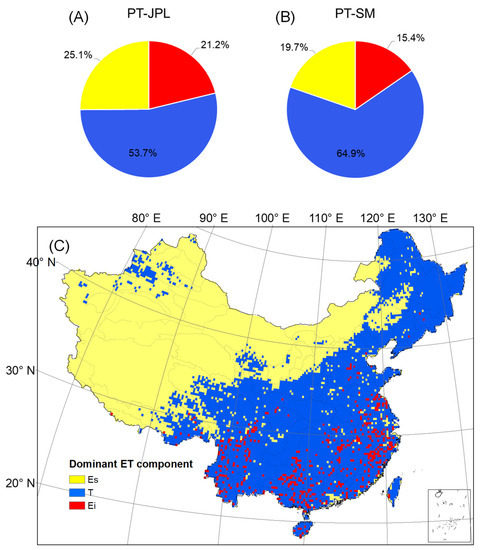
Figure 11.
Evapotranspiration (ET) components expressed as a percentage of total ET from (A) the original PT–JPL algorithm (PT–JPL) and (B) updated PT–SM algorithm across China. Yellow indicates soil evaporation (Es), blue indicates vegetation transpiration (T), and red indicates canopy interception evaporation (Ei). Below, (C) the spatial distribution of the dominant percent contribution to total ET from components as Es, T, and Ei.
Figure 11C reveals the spatial patterns of dominant ET components. It can be seen that the bare soil evaporation is dominated across almost the entire arid area of northwest China, especially in the arid and semi-arid regions, while in some warmer and wet regions, such as southeastern of Tibet, the interception loss is the main component. In contrast, transpiration typically takes up most of the remaining regions (especially the forested terrain), while in some areas in southern China (often rainforests), the total interception loss is generally the dominant component. These findings are consistent with the partitioning obtained from other datasets [6,24]. Nonetheless, this phenomenon is a comprehensive reflection of climate, water absorption capacity of vegetation, growth status, soil moisture, etc.
4.3. Inter-Annual Variability of ET for 2003–2015
It can be seen that the whole of China is characterized by complex spatial patterns in ET and its change in components (Figure 12). For the total ET, more than half of the entire area of China show upward trends, while the other half show downward trends. Additionally, the largest upward trend of the annual ET series is recognized at the Qinghai–Tibet Plateau with a value of 3.35 mm/y, while the largest downward trend (i.e., −2.88 mm/y) can be found at the southeastern part of China (Figure 12A). Moreover, based on a modified Priestley–Taylor algorithm, Yao et al. (2013) found that the LE decreased over large areas in central China, northwest China, and Inner Mongolia while increasing in the northeast, north, and south regions of China during the period of 2001–2010 by driving monthly MODIS products [29]. These two results are different partly due to the different study periods, and another reason could be the difference in data and methods used. By employing the ensembles of remote sensing-based physical models and machine learning algorithms, overall increasing trends (0.62 and 0.38 mm/y, respectively) in global terrestrial ET during the period of 1982–2011 were evaluated by Pan et al. (2020) [17]. A further investigation into the control factors of ET variations showed that anthropogenic Earth greening was the dominating factor, which has also been reported by previous studies [1,67]. By contrast, drought and reducing solar radiation caused by substantial increases in aerosol optical depth (AOD) were usually identified as the main possible factors of ET reduction [68,69].
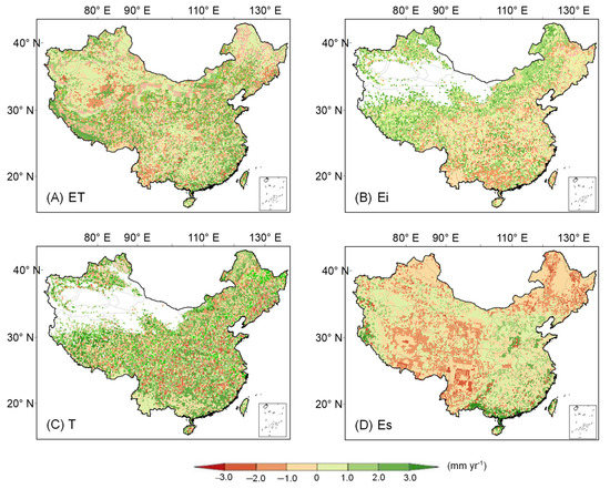
Figure 12.
Annual trend slopes of (A) PT–SM evapotranspiration (ET); (B) canopy evaporation (Ei); (C) vegetation transpiration (T); and (D) soil evaporation (Es) during 2003–2015.
The ET components are not only influenced by vegetation cover and growth period but also by environmental factors, such as climate conditions, topography, and soil characteristics [70]. However, the control degree of different influencing factors on individual ET components varies with energy and water conditions. Ei across northwest China indicates upward trends, and this may be a result of the afforestation and grassland projection over the past two decades. For almost the whole southeastern part of China, Ei shows downward trends with the largest downward trend (i.e., −2.57 mm/y) being found in central China (Figure 12B), this result is relatively reasonable due to the development of modern agricultural technology, a large number of agricultural water-saving technologies have been implemented in the southeast region, the water use efficiency was increased, and the unnecessary evaporation dissipation was reduced [71]. As for the vegetation T, most areas presented upward trends, except small areas in the northeastern and southeastern parts of the country, and the larger upward trends of annual T series were recognized at the Tibetan Plateau, with a value over 2.00 mm/y (Figure 12C). Unlike the general paradox regarding whether or not the growing-season precipitation amount or the precipitation pattern is the main reason for vegetation T change [6,72], increased NDVI and LAI as a result of large-scale afforestation and agricultural intensification have been widely identified to play the most important role in the increase in vegetation T [17,58,73]. Es across China (with the exception of the southeastern region) presented downward trends. Furthermore, the changing trends were mostly less than 3.00 mm/y (Figure 12D). Similar to Ei, Es also represents the ineffective water consumption that does not directly contribute to production. Although the slopes of the trends were different, all of the values of ET and its components have been found to show increasing trends with increasing precipitation by Gu et al. (2018) [58]. Meanwhile, the variation of fREW (relative extractable water) has the most significant impact on the Es simulation in arid areas with low vegetation [74]. Nevertheless, such Es reduction may be due to the decrease in solar radiation or drought. Additionally, many studies noted that the sensibility of ET components changes in relation to different climatic environments, biomasses, soil properties, plant types, and canopy heights [7,23,75]. Therefore, the reasons for the distinction of the performances of the updated PT-SM algorithm with a soil moisture constraint on Es and T separately are complex and warrant further investigation.
5. Conclusions
By incorporating soil moisture into the widely used PT-JPL ET algorithm, in this study, ET and its components series at a spatial scale of 0.25 × 0.25° were estimated. For this purpose, SM data at three layers (0–5, 5–20, and 20–100 cm) were firstly reconstructed by the multiple linear regression model and trapezoidal method, integrating the datasets of humidity observations relative to farmland soil, observed precipitation, GRACE solutions, and SM datasets obtained from the LDAS-2 outputs and Yang et al. (2020). High SM values generally occurred in the southeastern part of China, while low values were distributed in the northwestern part of the country. Meanwhile, the two algorithms’ parameters in the update PT-SM ET algorithm (fREW and fTRM) were compared with the parameters in the original PT-JPL algorithm (fsm and fM). The values of parameters in the updated PT-SM ET algorithm (i.e., fREW and fTRM) were observed to be larger than those of the original PT-JPL algorithm (i.e., fsm and fM), especially in the peak or valley values.
The updated algorithm (i.e., PT-SM) model shows increased R2 and NSE and reduced RMSE and Bias, with the greatest improvements occurring in water-limited regions. SM incorporation into Es can improve ET estimates by increasing R2 and NSE by 2% and 7%, respectively; RMSE and Bias were reduced by 20% and 3 mm, respectively; while SM incorporation into T improved ET estimates by increasing R2 and NSE by 4% and 18%, respectively. RMSE and Bias were reduced by 34% and 7 mm, respectively. These updated PT-SM ET estimates distinctly show a reduced error and provide a rich dataset to evaluate land surface models, vegetation or anthropogenic perturbation response to changes in water availability. The mean annual ET distribution presented an intricate spatial structure with relatively high ET values in the southeast of China and low values in the northwestern part. As a whole, the soil moisture constraint resulted in a higher transpiration estimate and lower evaporation estimate. These results can provide more accurate water consumption data for regional water resource management and planning. In the future, a high spatial–temporal resolution ET is expected to be obtained. Therefore, the critical variables determining the model’s ability to simulate ET components, vegetation, surface, and root-zone soil moisture at high spatial–temporal resolution, are urgently needed.
Author Contributions
Conceptualization, W.X. and W.W.; methodology, W.X.; software, L.S.; validation, W.X. and Q.S.; formal analysis, M.C.; investigation, W.X.; resources, W.W.; data curation, L.S.; writing—Original draft preparation, W.X.; writing—Review and editing, Q.S.; visualization, W.X.; supervision, Q.S.; project administration, W.W.; funding acquisition, W.X. All authors have read and agreed to the published version of the manuscript.
Funding
This work was jointly funded by the National Science Foundation of China (51809073), the National Key R&D Program of China (2018YFA0605402), the Fundamental Research Funds for the Central Universities (B200201005), and the Belt and Road Special Foundation of the State Key Laboratory of Hydrology-Water Resources and Hydraulic Engineering (2020490511).
Institutional Review Board Statement
Not applicable for studies not involving humans or animals.
Informed Consent Statement
Not applicable for studies not involving humans.
Data Availability Statement
The data that support the findings of this study are available from the corresponding author upon reasonable request.
Conflicts of Interest
The authors declare no conflict of interest.
References
- Wang, K.; Dickinson, R.E. A review of global terrestrial evapotranspiration: Observation, modeling, climatology, and climatic variability. Rev. Geophys. 2012, 50, RG2005. [Google Scholar] [CrossRef]
- Yuan, W.; Liu, S.; Yu, G.; Bonnefond, J.-M.; Chen, J.; Davis, K.; Desai, A.R.; Goldstein, A.H.; Gianelle, D.; Rossi, F.; et al. Global estimates of evapotranspiration and gross primary production based on MODIS and global meteorology data. Remote Sens. Environ. 2010, 114, 1416–1431. [Google Scholar] [CrossRef] [Green Version]
- Evaristo, J.; Jasechko, S.; Mcdonnell, J.J. Global separation of plant transpiration from groundwater and streamflow. Nature 2015, 525, 91–94. [Google Scholar] [CrossRef]
- Monteith, J.L.L. Evaporation and environment. Symp. Soc. Exp. Biol. 1965, 19, 205–234. [Google Scholar] [CrossRef] [PubMed] [Green Version]
- Priestley, C.H.B.; Taylor, R.J. On the assessment of surface heat fluxes and evaporation using large-scale parameters. Mon. Weather Rev. 1972, 100, 81–92. [Google Scholar] [CrossRef]
- Schlesinger, W.H.; Jasechko, S. Transpiration in the global water cycle. Agric. For. Meteorol. 2014, 189–190, 115–117. [Google Scholar] [CrossRef]
- Zhang, Y.; Kong, D.; Gan, R.; Chiew, F.H.S.; McVicar, T.R.; Zhang, Q.; Yang, Y. Coupled estimation of 500 m and 8-day resolution global evapotranspiration and gross primary production in 2002–2017. Remote Sens. Environ. 2019, 222, 165–182. [Google Scholar] [CrossRef]
- Rothfuss, Y.; Biron, P.; Braud, I.; Canale, L.; Durant, J.L.; Gaudet, J.P.; Richard, P.; Vauclin, M.; Bariac, T. Partitioning evapotranspiration fluxes into soil evaporation and plant transpiration using water stable isotopes under controlled conditions. Hydrol. Process. 2010, 24, 3177–3194. [Google Scholar] [CrossRef]
- Cavanaugh, M.L.; Kurc, S.A.; Scott, R.L. Evapotranspiration partitioning in semiarid shrubland ecosystems: A two-site evaluation of soil moisture control on transpiration. Ecohydrology 2011, 4, 671–681. [Google Scholar] [CrossRef]
- Ershadi, A.; McCabe, M.F.; Evans, J.P.; Chaney, N.W.; Wood, E.F. Multi-site evaluation of terrestrial evaporation models using FLUXNET data. Agric. For. Meteorol. 2014, 187, 46–61. [Google Scholar] [CrossRef]
- Sutanto, S.J.; van den Hurk, B.; Dirmeyer, P.A.; Seneviratne, S.I.; Röckmann, T.; Trenberth, K.E.; Blyth, E.M.; Wenninger, J.; Hoffmann, G. HESS opinions “A perspective on isotope versus non-isotope approaches to determine the contribution of transpiration to total evaporation”. Hydrol. Earth Syst. Sci. 2014, 18, 2815–2827. [Google Scholar] [CrossRef] [Green Version]
- McCabe, M.F.; Ershadi, A.; Jimenez, C.; Miralles, D.G.; Michel, D.; Wood, E.F. The GEWEX LandFlux project: Evaluation of model evaporation using tower-based and globally gridded forcing data. Geosci. Model Dev. 2016, 9, 283–305. [Google Scholar] [CrossRef] [Green Version]
- Aouade, G.; Jarlan, L.; Ezzahar, J.; Er-Raki, S.; Napoly, A.; Benkaddour, A.; Khabba, S.; Boulet, G.; Garrigues, S.; Chehbouni, A.; et al. Evapotranspiration partition using the multiple energy balance version of the ISBA-A-gs land surface model over two irrigated crops in a semi-arid Mediterranean region (Marrakech, Morocco). Hydrol. Earth Syst. Sci. 2020, 24, 3789–3814. [Google Scholar] [CrossRef]
- Scanlon, T.M.; Kustas, W.P. Partitioning carbon dioxide and water vapor fluxes using correlation analysis. Agric. For. Meteorol. 2010, 150, 89–99. [Google Scholar] [CrossRef]
- Kool, D.; Agam, N.; Lazarovitch, N.; Heitman, J.L.; Sauer, T.J.; Ben-Gal, A. A review of approaches for evapotranspiration partitioning. Agric. For. Meteorol. 2014, 184, 56–70. [Google Scholar] [CrossRef]
- Maxwell, R.M.; Condon, L.E. Connections between groundwater flow and transpiration partitioning. Science 2016, 353, 377–380. [Google Scholar] [CrossRef] [PubMed] [Green Version]
- Pan, S.; Pan, N.; Tian, H.; Friedlingstein, P.; Sitch, S.; Shi, H.; Arora, V.K.; Haverd, V.; Jain, A.K.; Kato, E.; et al. Evaluation of global terrestrial evapotranspiration using state-of-the-art approaches in remote sensing, machine learning and land surface modeling. Hydrol. Earth Syst. Sci. 2020, 24, 1485–1509. [Google Scholar] [CrossRef] [Green Version]
- Cui, Y.; Jia, L.; Fan, W. Estimation of actual evapotranspiration and its components in an irrigated area by integrating the Shuttleworth-Wallace and surface temperature-vegetation index schemes using the particle swarm optimization algorithm. Agric. For. Meteorol. 2021, 307, 108488. [Google Scholar] [CrossRef]
- Jung, M.; Reichstein, M.; Ciais, P.; Seneviratne, S.I.; Sheffield, J.; Goulden, M.L.; Bonan, G.; Cescatti, A.; Chen, J.; de Jeu, R.; et al. Recent decline in the global land evapotranspiration trend due to limited moisture supply. Nature 2010, 467, 951–954. [Google Scholar] [CrossRef]
- Mu, Q.; Zhao, M.; Running, S.W. Improvements to a MODIS global terrestrial evapotranspiration algorithm. Remote Sens. Environ. 2011, 115, 1781–1800. [Google Scholar] [CrossRef]
- Cleugh, H.A.; Leuning, R.; Mu, Q.; Running, S.W. Regional evaporation estimates from flux tower and MODIS satellite data. Remote Sens. Environ. 2007, 106, 285–304. [Google Scholar] [CrossRef]
- Mu, Q.; Heinsch, F.A.; Zhao, M.; Running, S.W. Development of a global evapotranspiration algorithm based on MODIS and global meteorology data. Remote Sens. Environ. 2007, 111, 519–536. [Google Scholar] [CrossRef]
- Miralles, D.G.; De Jeu, R.A.M.; Gash, J.H.; Holmes, T.R.H.; Dolman, A.J. Magnitude and variability of land evaporation and its components at the global scale. Hydrol. Earth Syst. Sci. 2011, 15, 967–981. [Google Scholar] [CrossRef] [Green Version]
- Purdy, A.J.; Fisher, J.B.; Goulden, M.L.; Colliander, A.; Halverson, G.; Tu, K.; Famiglietti, J.S. SMAP soil moisture improves global evapotranspiration. Remote Sens. Environ. 2018, 219, 1–14. [Google Scholar] [CrossRef]
- Talsma, C.J.; Good, S.P.; Jimenez, C.; Martens, B.; Fisher, J.B.; Miralles, D.G.; McCabe, M.F.; Purdy, A.J. Partitioning of evapotranspiration in remote sensing-based models. Agric. For. Meteorol. 2018, 260–261, 131–143. [Google Scholar] [CrossRef]
- Daly, E.; Porporato, A. A review of soil moisture dynamics: From rainfall infiltration to ecosystem response. Environ. Eng. Sci. 2005, 22, 9–24. [Google Scholar] [CrossRef]
- Gu, H.; Lin, Z.; Guo, W.; Deb, S. Retrieving surface soil water content using a soil texture adjusted vegetation index and unmanned aerial system images. Remote Sens. 2021, 13, 145. [Google Scholar] [CrossRef]
- Hain, C.R.; Crow, W.T.; Mecikalski, J.R.; Anderson, M.C.; Holmes, T. An intercomparison of available soil moisture estimates from thermal-infrared and passive microwave remote sensing and land-surface modeling. J. Geophys. Res. 2011, 116, D15107. [Google Scholar] [CrossRef]
- Yao, Y.; Liang, S.; Cheng, J.; Liu, S.; Fisher, J.B.; Zhang, X.; Jia, K.; Zhao, X.; Qin, Q.; Zhao, B.; et al. MODIS-driven estimation of terrestrial latent heat flux in China based on a modified Priestley-Taylor algorithm. Agric. For. Meteorol. 2013, 171–172, 187–202. [Google Scholar] [CrossRef]
- Fernández-Prieto, D.; van Oevelen, P.; Su, Z.; Wagner, W. Advances in earth observation for water cycle science. Hydrol. Earth Syst. Sci. 2012, 16, 543–549. [Google Scholar] [CrossRef]
- Rebel, K.T.; de Jeu, R.A.M.; Ciais, P.; Viovy, N.; Piao, S.L.; Kiely, G.; Dolman, A.J. A global analysis of soil moisture derived from satellite observations and a land surface model. Hydrol. Earth Syst. Sci. 2012, 16, 833–847. [Google Scholar] [CrossRef] [Green Version]
- Walker, E.; García, G.A.; Venturini, V.; Carrasco, A. Regional evapotranspiration estimates using the relative soil moisture ratio derived from SMAP products. Agric. Water Manag. 2019, 216, 254–263. [Google Scholar] [CrossRef]
- Jackson, T.J.; Bindlish, R.; Cosh, M.H.; Zhao, T.; Starks, P.J.; Bosch, D.D.; Leroux, D. Validation of soil moisture and ocean salinity (SMOS) soil moisture over watershed networks in the US. IEEE Trans. Geosci. Remote Sens. 2012, 50, 1530–1543. [Google Scholar] [CrossRef] [Green Version]
- Sadeghi, M.; Gao, L.; Ebtehaj, A.; Wigneron, J.P.; Crow, W.T.; Reager, J.T.; Warrick, A.W. Retrieving global surface soil moisture from GRACE satellite gravity data. J. Hydrol. 2020, 124717. [Google Scholar] [CrossRef]
- Zhang, Q.; Yuan, Q.; Li, J.; Wang, Y.; Sun, F.; Zhang, L. Generating seamless global daily AMSR2 soil moisture (SGD-SM) long-term products for the years 2013–2019. Earth Syst. Sci. Data 2021, 13, 1385–1401. [Google Scholar] [CrossRef]
- Xing, W.; Wang, W.; Shao, Q.; Yong, B.; Liu, C.; Feng, X.; Dong, Q. Estimating monthly evapotranspiration by assimilating remotely sensed water storage data into the extended Budyko framework across different climatic regions. J. Hydrol. 2018, 567, 684–695. [Google Scholar] [CrossRef]
- Fisher, J.B.; Tu, K.P.; Baldocchi, D.D. Global estimates of the land-atmosphere water flux based on monthly AVHRR and ISLSCP-ii data, validated at 16 FLUXNET sites. Remote Sens. Environ. 2008, 112, 901–919. [Google Scholar] [CrossRef]
- Novick, K.A.; Ficklin, D.L.; Stoy, P.C.; Williams, C.A.; Bohrer, G.; Oishi, A.C.; Papuga, S.A.; Blanken, P.D.; Noormets, A.; Sulman, B.N.; et al. The increasing importance of atmospheric demand for ecosystem water and carbon fluxes. Nat. Clim. Chang. 2016, 6, 1023–1027. [Google Scholar] [CrossRef] [Green Version]
- Fan, X.; Liu, Y.; Gan, G.; Wu, G. SMAP underestimates soil moisture in vegetation-disturbed areas primarily as a result of biased surface temperature data. Remote Sens. Environ. 2020, 247, 111914. [Google Scholar] [CrossRef]
- Martens, B.; Miralles, D.G.; Lievens, H.; Van Der Schalie, R.; De Jeu, R.A.M.; Fernández-Prieto, D.; Beck, H.E.; Dorigo, W.A.; Verhoest, N.E.C. GLEAM v3: Satellite based land evaporation and root-zone soil moisture. Geosci. Model Dev. 2017, 10, 1903–1925. [Google Scholar] [CrossRef] [Green Version]
- Anderson, M.C.; Norman, J.M.; Mecikalski, J.R.; Otkin, J.A.; Kustas, W.P. A climatological study of evapotranspiration and moisture stress across the continental United States based on thermal remote sensing: 1. Model formulation. J. Geophys. Res. 2007, 112, D10117. [Google Scholar] [CrossRef]
- Van Diepen, C.A.; Wolf, J.; van Keulen, H.; Rappoldt, C. WOFOST: A simulation model of crop production. Soil Use Manag. 1989, 5, 16–24. [Google Scholar] [CrossRef]
- Foken, T. The energy balance closure problem: An overview. Ecol. Appl. 2008, 18, 1351–1367. [Google Scholar] [CrossRef]
- Twine, T.E.; Kustas, W.P.; Norman, J.M.; Cook, D.R.; Houser, P.R.; Meyers, T.P.; Prueger, J.H.; Starks, P.J.; Wesely, M.L. Correcting eddy-covariance flux underestimates over a grassland. Agric. For. Meteorol. 2000, 103, 279–300. [Google Scholar] [CrossRef] [Green Version]
- He, J.; Yang, K.; Tang, W.; Lu, H.; Qin, J.; Chen, Y.Y.; Li, X. The first high-resolution meteorological forcing dataset for land process studies over China. Sci. Data 2020, 7, 25. [Google Scholar] [CrossRef] [PubMed] [Green Version]
- Simard, M.; Pinto, N.; Fisher, J.B.; Baccini, A. Mapping forest canopy height globally with spaceborne lidar. J. Geophys. Res. Biogeosci. 2011, 116. [Google Scholar] [CrossRef] [Green Version]
- Ek, M.; Mitchell, K.; Lin, Y.; Rogers, E.; Grunmann, P.; Koren, V.; Gayno, G.; Tarpley, J.D. Implementation of Noah land surface model advances in the National Centers for Environmental Prediction operational mesoscale Eta model. J. Geophys. Res. 2003, 108, D22. [Google Scholar] [CrossRef]
- Mittelbach, H.; Lehner, I.; Seneviratne, S.I. Comparison of four soil moisture sensor types under field conditions in Switzerland. J. Hydrol. 2012, 430–431, 39–49. [Google Scholar] [CrossRef]
- Yang, K.; Chen, Y.; He, J.; Zhao, L.; Lu, H.; Qin, J.; Zheng, D.H.; Li, X. Development of a daily soil moisture product for the period of 2002–2011 in Chinese Mainland. Sci. China Earth Sci. 2020, 63, 1113–1125. [Google Scholar] [CrossRef]
- Swenson, S. GRACE Monthly Mass Grids-Land; Jet Propulsion Laboratory: Pasadena, CA, USA, 2014. [Google Scholar]
- Mohamed, S.O.; Bertuzzi, P.; Bruand, A.; Raison, L.; Bruckler, L. Field evaluation and error analysis of soil water content measurement using the capacitance probe method. Soil Sci. Soc. Am. J. 1997, 61, 399–408. [Google Scholar] [CrossRef]
- Yu, Z.; Liu, D.; Lü, H.; Fu, X.; Xiang, L.; Zhu, Y. A multi-layer soil moisture data assimilation using support vector machines and ensemble particle filter. J. Hydrol. 2012, 475, 53–64. [Google Scholar] [CrossRef]
- Hirschi, M.; Mueller, B.; Dorigo, W.; Seneviratne, S.I. Using remotely sensed soil moisture for land-atmosphere coupling diagnostics: The role of surface vs. root-zone soil moisture variability. Remote Sens. Environ. 2014, 154, 246–252. [Google Scholar] [CrossRef] [Green Version]
- Fu, T.; Chen, H.; Zhang, W.; Nie, Y.; Gao, P.; Wang, K. Spatial variability of surface soil saturated hydraulic conductivity in a small karst catchment of southwest China. Environ. Earth Sci. 2015, 74, 2381–2391. [Google Scholar] [CrossRef]
- Wang, A.; Lettenmaier, D.P.; Sheffield, J. Soil moisture drought in China, 1950–2006. J. Clim. 2011, 24, 3257–3271. [Google Scholar] [CrossRef]
- Liu, J.G.; Xie, Z.H. Improving simulation of soil moisture in China using a multiple meteorological forcing ensemble approach. Hydrol. Earth Syst. Sci. 2013, 17, 3355–3369. [Google Scholar] [CrossRef] [Green Version]
- Miralles, D.G.; Gash, J.H.; Holmes, R.H.; De Jeu, R.A.M.; Dolman, A.J. Global canopy interception from satellite observations. J. Geophys. Res. 2010, 115, D16122. [Google Scholar] [CrossRef]
- Gu, C.; Ma, J.; Zhu, G.; Yang, H.; Zhang, K.; Wang, Y.; Gu, C. Partitioning evapotranspiration using an optimized satellite-based ET model across biomes. Agric. For. Meteorol. 2018, 259, 355–363. [Google Scholar] [CrossRef]
- Llorens, P.; Domingo, F. Rainfall partitioning by vegetation under Mediterranean conditions. A review of studies in Europe. J. Hydrol. 2007, 335, 37–54. [Google Scholar] [CrossRef]
- Jasechko, S.; Sharp, Z.D.; Gibson, J.J.; Birks, S.J.; Yi, Y.; Fawcett, P.J. Terrestrial water fluxes dominated by transpiration. Nature 2013, 496, 347–350. [Google Scholar] [CrossRef] [PubMed]
- Wang, H.; Tetzlaff, D.; Dick, J.J.; Soulsby, C. Assessing the environmental controls on Scots pine transpiration and the implications for water partitioning in a boreal headwater catchment. Agric. For. Meteorol. 2017, 240–241, 58–66. [Google Scholar] [CrossRef] [Green Version]
- Al-Hamdan, O.Z.; Cruise, J.F. Soil moisture profile development from surface observations by principle of maximum entropy. J. Hydrol. Eng. 2010, 15, 327–337. [Google Scholar] [CrossRef]
- Dorigo, W.A.; Gruber, A.; De Jeu, R.A.M.; Wagner, W.; Stacke, T.; Loew, A.; Kidd, R. Evaluation of the ESA CCI soil moisture product using ground-based observations. Remote Sens. Environ. 2015, 162, 380–395. [Google Scholar] [CrossRef]
- Gill, M.K.; McKee, M. Soil moisture data assimilation using support vector machines and ensemble Kalman filter. J. Am. Water Resour. Assoc. 2007, 43, 1004–1015. [Google Scholar] [CrossRef]
- Monsivais-Huertero, A.; Graham, W.D.; Judge, J.; Agrawal, D. Effect of simultaneous state-parameter estimation and forcing uncertainties on rootzone soil moisture for dynamic vegetation using EnKF. Adv. Water Resour. 2010, 33, 468–484. [Google Scholar] [CrossRef]
- Li, Y.; Piao, S.; Li, L.Z.X.; Chen, A.; Wang, X.; Ciais, P.; Huang, L.; Lian, X.; Peng, S.; Zeng, Z.; et al. Divergent hydrological response to large-scale afforestation and vegetation greening in China. Sci. Adv. 2018, 4, eaar4182. [Google Scholar] [CrossRef] [Green Version]
- Zhang, K.; Kimball, J.S.; Nemani, R.R.; Running, S.W.; Hong, Y.; Gourley, J.J.; Yu, Z. Vegetation greening and climate change promote multidecadal rises of global land evapotranspiration. Sci. Rep. 2015, 5, 15956. [Google Scholar] [CrossRef] [PubMed]
- Zhao, M.; Running, S.W. Drought-induced reduction in global terrestrial net primary production from 2000 through 2009. Science 2010, 329, 940–943. [Google Scholar] [CrossRef] [Green Version]
- Zheng, X.B.; Zhou, C.X.; Luo, Y.X.; Chen, J.; Zhao, T.L. Chinese province-level variations and trends in aerosol optical depth from recent 10 years of remote sensing data. Ecol. Environ. Sci. 2011, 20, 595–599. (In Chinese) [Google Scholar]
- Milly, P.C.D.; Dunne, K.A. Potential evapotranspiration and continental drying. Nat. Clim. Chang. 2016, 6, 946–949. [Google Scholar] [CrossRef]
- Tang, X.; Li, H.; Desai, A.R.; Nagy, Z.; Luo, J.; Kolb, T.E.; Olioso, A.; Xu, X.; Yao, L.; Kutsch, W. How is water-use efficiency of terrestrial ecosystems distributed and changing on Earth? Sci. Rep. 2014, 4, 7483. [Google Scholar] [CrossRef]
- Moran, M.S.; Scott, R.L.; Keefer, T.O.; Emmerich, W.E.; Hernandez, M.; Nearing, G.S.; Paige, G.B.; Cosh, M.H.; O’Neill, P.E. Partitioning evapotranspiration in semiarid grassland and shrubland ecosystems using time series of soil surface temperature. Agric. For. Meteorol. 2009, 149, 59–72. [Google Scholar] [CrossRef]
- Zhou, S.; Yu, B.; Zhang, Y.; Huang, Y.; Wang, G. Partitioning evapotranspiration based on the concept of underlying water use efficiency. Water Resour. Res. 2016, 52, 1160–1175. [Google Scholar] [CrossRef] [Green Version]
- Zhang, K.; Ma, J.; Zhu, G.; Ma, T.; Han, T.; Feng, L.L. Parameter sensitivity analysis and optimization for a satellite-based evapotranspiration model across multiple sites using Moderate Resolution Imaging Spectroradiometer and flux data. J. Geophys. Res. Atmos. 2017, 122, 230–245. [Google Scholar] [CrossRef]
- Fan, Y.; Miguez-Macho, G.; Jobbágy, E.G.; Jackson, R.B.; Otero-Casal, C. Hydrologic regulation of plant rooting depth. Proc. Natl. Acad. Sci. USA 2017, 114, 10572–10577. [Google Scholar] [CrossRef] [PubMed] [Green Version]
Publisher’s Note: MDPI stays neutral with regard to jurisdictional claims in published maps and institutional affiliations. |
© 2021 by the authors. Licensee MDPI, Basel, Switzerland. This article is an open access article distributed under the terms and conditions of the Creative Commons Attribution (CC BY) license (https://creativecommons.org/licenses/by/4.0/).