Abstract
Building extraction is a basic task in the field of remote sensing, and it has also been a popular research topic in the past decade. However, the shape of the semantic polygon generated by semantic segmentation is irregular and does not match the actual building boundary. The boundary of buildings generated by semantic edge detection has difficulty ensuring continuity and integrity. Due to the aforementioned problems, we cannot directly apply the results in many drawing tasks and engineering applications. In this paper, we propose a novel convolutional neural network (CNN) model based on multitask learning, Dense D-LinkNet (DDLNet), which adopts full-scale skip connections and edge guidance module to ensure the effective combination of low-level information and high-level information. DDLNet has good adaptability to both semantic segmentation tasks and edge detection tasks. Moreover, we propose a universal postprocessing method that integrates semantic edges and semantic polygons. It can solve the aforementioned problems and more accurately locate buildings, especially building boundaries. The experimental results show that DDLNet achieves great improvements compared with other edge detection and semantic segmentation networks. Our postprocessing method is effective and universal.
1. Introduction
The automatic extraction and analysis of buildings from high-resolution remote-sensing images is an important research topic in the field of remote sensing [1,2,3]. The results are widely used in urban and rural planning, sociology, change detection [4], natural disaster assessment and other fields and are also important for updating geographic information databases [5]. Compared with natural images, high-resolution remote-sensing images have richer spatial, spectral, and texture feature information. The rapid development of deep learning and computer vision has provided strong technical support for the analysis and use of high-resolution remote-sensing images [6]. Compared with artificial remote-sensing interpretation and vectorization, the CNN model can automatically extract buildings from remote-sensing images, which greatly reduces the consumption of human and material resources. However, due to the complex characteristics and background of geographic objects (geo-objects) [7], cases in which different geo-objects have the same spectrum or the same geo-objects have different spectra are commonly encountered, which makes accurate pixel-level classification a difficult problem. In addition, problems such as cloud, tree and shadow occlusion [4,8], different imaging angles [9], difficulty in drawing labels, and label omissions hinder the accurate estimation of buildings by CNN. Using the characteristics of high-resolution remote-sensing images to perform tasks such as image recognition and detection while avoiding the negative effects of redundant information has become the most challenging frontier issue in the field of remote sensing.
In high-resolution remote-sensing images, buildings are geo-objects with artificial features, rich in types and semantic information, which are great differences in scale, architectural style, and form. It is difficult to ensure the accuracy of building location that depending on high-level semantic features and the accuracy of building boundary that depending on low-level edge features. Currently, most building extraction algorithms are based on semantic segmentation and semantic edge detection.
With the development of deep learning, edge detection algorithm has developed rapidly. HED [10] uses a fully convolutional network with deep supervision to automatically learn multilevel representations and effectively solve the problem of edge ambiguity. However, HED only considers the last convolutional layer information of each stage, while RCF [11] makes full use of multiscale and multilevel information of all convolutional layers. BDCN [12] introduced the scale enhancement module to use multiscale representations to improve the edge detection capabilities. DFF [13] adaptively assigns appropriate fusion weights strategy which helps to produce more accurate and clear edge predictions. CaseNet [14] is an end-to-end semantic edge network based on ResNet [15] that proposes a new skip layer in which the category edge activations of the top layer share and merge the same group features.
The rapid development of deep learning edge detection algorithms provides strong support for building edge detection in high-resolution remote-sensing images. Reda et al. [16] proposed a faster edge region convolutional neural network (FER-CNN). FER-CNN uses the parametric rectified linear unit (PReLu) [17] activation function, which adds only a very small number of parameters to improve the edge detection of buildings. Lu et al. [2] adopted a building edge detection model based on RCF [11], which obtains the edge strength map through the RCF and then refines the edge strength map according to the geometric analysis of the terrain surface. Semantic edge detection which aims at extracting edges as well as semantic information can generate an edge strength map to describe the confidence of the predicted building boundary, but complete edges are difficult to guarantee, and incomplete edges are not sufficient to support the accurate extraction of buildings.
Semantic segmentation is a joint task that requires the positioning and classification of both spatial information and semantic information, paving the way for a complete understanding of the scene. FCN [18] uses the concept of full convolution to perform end-to-end semantic segmentation, and it creatively employs a skip connection that combines high-level information with low-level information to improve segmentation. U-Net [19] modified and expanded the FCN that adds an upsampling stage and a feature channel fuse strategy that uses a connection operation to directly pass high-level information from an encoder to the decoder of the same height. SegNet [20] performs forward evaluation of the fully learned function to obtain smooth predictions and increases the depth of the network so that the network can consider the larger context information. RefineNet [21] is a multipath optimization network that refines low-resolution semantic features in a recursive manner, and proposes a chain residual pool that can capture the context of the background. PSPNet [22] expand the receptive field by dilated convolution to obtain feature maps that can acquire the global scene. PSPNet perform pooling at different levels, and then fuse the local information and global context information.
The powerful feature extraction and interpretation ability of semantic segmentation provides a new method for the interpretation of high-resolution remote-sensing images, which is helpful for the accurate extraction and positioning of buildings and reduces the problems of false extraction and missing detection of buildings. Liu et al. [23] proposed a spatial residual inception network (SRI-Net), in which an SRI module captures and aggregates multiscale contexts for semantic understanding by successively fusing multilevel features. SRI-Net is capable of accurately detecting large buildings while retaining global morphological characteristics and local details. Delassus et al. [24] proposed a fusion strategy based on U-Net [19], which combines the segmented output of the combined model and multiple channels of the input image. Lin et al. [25] proposed an efficient separable factorized network (ESFNet), which uses separable residual blocks and dilated convolution to maintain a small loss of accuracy as well as low computational cost and memory consumption. At the same time, the high precision of semantic segmentation is maintained. Yi et al. [7] proposed a ResUNet based on U-Net and Resnet. It uses a deep residual learning method to promote training and alleviate the problem of model training degradation. Shuang Wang [26] proposed a full convolutional network with dense connections that designed top-down short connections to facilitate the fusion of high and low feature information. However, there are usually irregular boundaries that are difficult to completely match the boundaries of the actual building, and it is impossible to effectively distinguish adjacent buildings [5].
Multitask learning is a learning mechanism inspired by human beings to acquire knowledge of complex tasks by performing different shared subtasks simultaneously [27]. Its aim is to leverage useful information contained in related tasks to help improve the generalization performance of all the tasks [28]. Multitask learning is currently a mainstream direction of deep learning. At present, there are some methods that use multitask learning to integrate edge information and semantic information in CNN to output semantic polygons with precise edges. Even if deep learning methods are widely used in high-resolution remote-sensing building extraction, it is still a challenging task to achieve the precise extraction of building.
Inspired by the multitask learning and the aforementioned problems of semantic edge detection and semantic segmentation in building extraction, we designed a novel CNN model based on multitask learning to achieve accurate extraction of buildings, Dense D-LinkNet (DDLNet), based on D-LinkNet [29] and DenseNet [30]. DDLNet has good adaptability to both semantic segmentation tasks and semantic edge detection tasks. A new universal postprocessing method focuses on the complementarity between edge information and semantic information. The main contributions of this work are as follows.
- We designed a CNN model named Dense D-LinkNet (DDLNet) to extract buildings from high-resolution remote-sensing images. This model uses full-scale skip connections and edge guidance module to ensure the effective combination of low-level information and high-level information. DDLNet can adapt to both semantic segmentation tasks and edge detection tasks. DDLNet can effectively solve the problem of boundary blur and the problem of edge disconnection.
- We proposed an effective and universal postprocessing method that can effectively combine edge information and semantic information to improve the final result. Semantic polygon from the semantic segmentation to accurately locate and classify buildings at the pixel level. semantic edges from semantic edge detection to extract precise edges of buildings. This method uses semantic polygons to solve the problem of incompleteness of semantic edges and uses semantic edges to improve the boundary of semantic polygons, realize the accurate extraction of buildings.
2. Materials and Methods
The main purpose of this article is to overcome the incompleteness of edges from semantic edge detection and the problem of boundary blur from semantic segmentation and realize the precise extraction of buildings from remote-sensing images.
In this paper, we designed a novel CNN model Dense D-LinkNet (DDLNet), which can adapt to semantic segmentation tasks and semantic edge detection tasks. In addition, we propose a new postprocessing method to effectively fuse edge and semantic information and achieve the precise extraction of buildings from high-resolution remote-sensing images. The process of extracting buildings can be divided into three stages, as shown in Figure 1. First, the high-resolution remote-sensing images are labeled, and then the vector data are gridded into line label and polygon label, respectively. Second, DDLNet are trained and predicted to generate edge strength maps and semantic polygons, respectively. Then, in the postprocessing stage, edge information is used to improve the boundary of the semantic polygon to achieve more accurate boundary positioning, and the semantic polygon is used to repair discontinuous edges to ensure the continuity and integrity of the edge. Supplemented by the application of the watershed algorithm, semantic information is used as the seed point to select the result of the building to ensure the accuracy of the positioning and topological structure of the building.
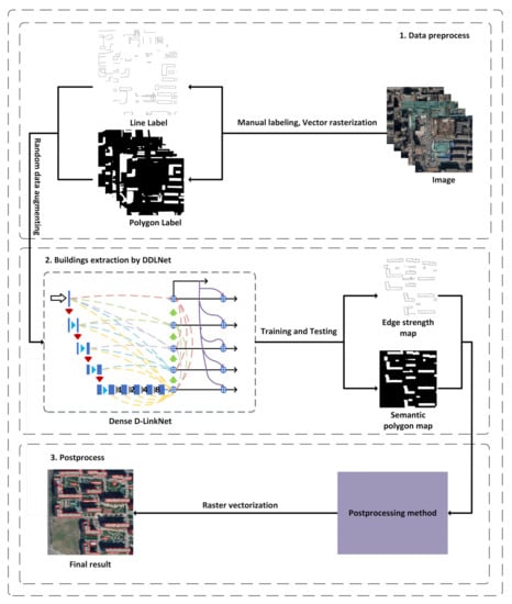
Figure 1.
Overall architecture of our method. This architecture can be divided into three stages. The first stage is data preprocessing, the second stage is deep learning training and prediction, which are used for DDLNet to generate edge strength maps and semantic polygons. The last stage is postprocessing, which is used for fusing edge and semantic information to obtain more accurate building results.
2.1. Dense D-LinkNet
Dense D-LinkNet (DDLNet) keeps the D-LinkNet [29] core structure and adds a full-scale skip connection, deep multiscale supervision, edge guidance module on this basis. D-LinkNet is built with the LinkNet [30] for road extraction tasks and adds dilated convolution layers in its center part. The encoder-decoder structure is the core of D-LinkNet. The encoder with pooling layers increases the receptive field but loses low-level details at the same time [5]. It is difficult to recover lost features with only the upsampling operation of the decoder. D-LinkNet only directly maps the features from the encoder to the corresponding decoder. Inspired by DenseNet [31] and U-Net3+ [32], we add the full-scale skip connection which is used to combine all the underlying low-level details with the decoder features to produce more accurate results. What’s more, the edge guidance module and deep multiscale supervision are also used to produce more accurate results. The structure of DDLNet is shown in Figure 2.
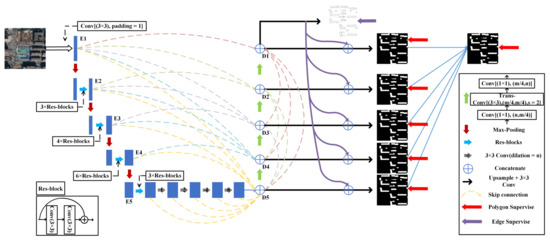
Figure 2.
Dense D-LinkNet architecture. Each blue block represents a multichannel feature. Left is the encoder, and the right is the decoder. The dotted curves represent full-scale skip connection. The purple curves represent edge guidance module. Each convolution layer is activated by ReLU, except the last convolution layer, which uses sigmoid activation.
2.1.1. Full-Scale Skip Connections
D-LinkNet just uses the skip connection to combine the same-scale feature from encoder to decoder at the same height. Our full-scale skip connections incorporate low-level details with high-level semantics from feature maps at different scales. Each decoder layer in DDLNet contains larger and same-scale feature maps from the encoder and smaller-scale feature maps from the decoder, which capture fine-grained details and coarse-grained semantics at full scales [32]. We mark the five encoding layers of the encoder as E1, E2, E3, E4, E5 from top to bottom, and mark the five decoding layers of the decoder as D1, D2, D3, D4, D5 from top to bottom, simultaneously. In Figure 2, we have made the corresponding mark. Each decoding layer combines low-level edge features and high-level semantic features through channel concatenate. Therefore, the D1 is the combination of E1, D2, D3, D4, D5. D2 is the combination of E1, E2, D3, D4, D5. D3 is the combination of E1, E2, E3, D4, D5. D4 is the combination of E1, E2, E3, E4, D5. D5 is the combination of E1, E2, E3, E4, and the features of E5 after a series of dilated convolutions.
It is well known that low-level features have richer details, while high-level features have richer semantic information. Therefore, the features after combination have both rich semantic information and spatial details [33]. This means that the full-scale features from the encoder can be used to improve the features in the decoder and the final result which contains high-precision boundary and semantic information.
2.1.2. Deep Multiscale Supervision
To learn hierarchical representations from multiscale feature, deep multiscale supervision is adopted in DDLNet. Multiscale objects are also a challenge for CNN. Currently, the extraction of target feature is conducted on a certain scale because of receptive field of convolution. Different levels have dissimilar high-level information and dissimilar low-level information [4].The feature map from each decoder layer (D1, D2, D3, D4, D5) should be predicted, and loss could be calculated with the groundtruth separately to realize detection at different scales, which is conducive to achieving deep supervision of each layer of the decoder and enhancing the learning ability [33]. Feature fusion is of great help to the promotion of targets at different scales.
The final polygon output is fused with each layer, as shown in Equation (1),
Here, is the predicted polygon result, subscript i is the number of each scale and subscript final represents the final polygon output, and w is the weight to fuse the polygon output of the layer. We choose w = 0.2 for each polygon output.
2.1.3. Edge Guidance Module
In this module, we aim to extract the precise edge features, then leverage the edge features to guide the polygon features to perform better on both segmentation and boundary. To obtain precise edge features, we decided to perform the edge supervise at the last layer of the decoder. It is well known that low-level features have richer details. However, only low-level information is not enough, while high-level semantic information also needed. The last layer of the decoder (D1) that contains the low-level features from the corresponding encoder and full-scale high-level features from the previous decoder is appropriate and effective for edge detection.
After obtaining the edge feature and polygon features, we aim to leverage the edge features to guide the polygon features. In our module, we propose the one-to-one guidance method. The polygon features from different decoder layer (D2, D3, D4, D5) need to be upsampled to the size of the edge feature and the combination of edge feature and each polygon feature is realized by channel concatenation. By fusing the edge feature into polygon features, the location of high-level predictions is more accurate, and more importantly, the boundary details become better.
2.1.4. Loss
Semantic Edge Loss: In end-to-end training, the loss function is computed over all pixels in a training image X and edge label Y. For a typical high-resolution remote-sensing image, the distribution of edge/nonedge pixels is heavily biased: 90% of the groundtruth is nonedged and 10% is edge [10]. HED introduces a class-balancing weight to offset this imbalance between edges and nonedges. HED defines the following class-balanced cross-entropy (CBCE) loss function used in Equation (2):
where and . and denote the edge and nonedge, respectively, denote the number of pixels. is the prediction map, and subscript j ∈ [0, 1, … H × W].
Currently, most edge detection networks, such as RCF, BDCN, and DexiNed, use the CBCE loss function to achieve edge detection for natural images. However, for high-resolution remote-sensing images, the CBCE loss will produce fuzzy and rough edges that cannot satisfy the requirement of drawing tasks and engineering applications. Therefore, we use the class-balanced mean square error (CMSE) loss that add the class-balanced parameter based on MSE loss. The CMSE loss can generate thin edge strength maps that are plausible for human eyes. The CMSE loss represents the sum of squares of the differences between the predicted value and the target value and then averages them. Equation (3) for CMSE loss is as follows: m = H × W, :
Semantic Segmentation Loss: For semantic segmentation, we used binary cross-entropy (BCE) and dice coefficient loss as the loss function. The formula of BCE loss as show in Equation (4).
The dice coefficient is a set similarity measure function, which is usually used to calculate the similarity of two samples, and the value range is [0, 1]. The formula of dice loss is shown in Equation (5):
is the intersection between and . and sub tables represent the number of elements of and , where the molecular coefficient is 2. The total loss can use the following Equation (6) to represent:
A major challenge in multitask learning comes from the optimization process itself. In particular, we need to carefully balance the joint training process of all tasks to avoid the situation that one or more tasks have a dominant influence in the network weights. In extreme cases, when the loss of one task is very large and the loss of other tasks is very small, the multitask is almost degenerated into single task goal learning, and the weight of the network is almost completely updated according to the large loss task, gradually losing the advantage of multitask learning. Therefore, we need the weight to balance semantic edge loss and semantic segmentation loss. The formula of final weighted loss is shown in Equation (7):
where is the weight of semantic edge loss and is the weight of semantic segmentation loss. We observed the final loss convergence of the DDLNet and determined that = 100, = 6 are suitable parameters.
2.2. Postprocessing
To fully fuse edge information and semantic information, complementary information is used to obtain better prediction results and achieve the precise extraction of buildings. We propose a new postprocessing method.
The semantic edge detection networks and semantic segmentation networks are used to generate the edge strength maps and semantic polygon results, respectively. The prediction image is a grayscale image with pixel values in the range of 0 to 255. The choice of binarization threshold is crucial. Considering that our postprocessing method can remove redundant pixels and more pixels are needed to ensure the results. Thus, we choose the threshold of 100 instead of the threshold of 127 as usual. After binarization, multipixel-width edges cannot represent the building edges. Therefore, we use a skeleton extraction algorithm to refine the edges to a single-pixel width and delete some of the broken lines that exist separately. Thus, we obtained a single-pixel edge map (as shown in Figure 3a) and a binary semantic polygon (as shown in Figure 3b).
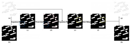
Figure 3.
Postprocessing flow chart. (a) is a single-pixel edge map, and (b) is a semantic polygon map. (c) is the result in which Equation (8) is used to overlay edges on the semantic polygon. (d) is the result in which the watershed algorithm is used to extract the boundaries. (e) is the result in which Equation (9) is used to add edges on the semantic polygon. (f) is a complete semantic polygon. (g) is the final edge result, and (h) is the final semantic segmentation result. The most obvious improvement is indicated by the circle. The blue line represents the effect of Equation (8) and the watershed algorithm, and the yellow line represents the effect of Equation (9) and hole filling.
The problem of edge discontinuity can be solved by the integrity of the semantic polygon. The problem of inaccurate boundaries of semantic polygons can be solved by semantic edges. The improvement in the semantic polygon boundaries is mainly reflected in the following two aspects of our method:
- If the boundary of the semantic polygon is beyond the edge of a single pixel, it needs to be deleted.
- If the boundary of the semantic polygon is within the boundary of a single pixel, it needs to be supplemented.
In the first case, we propose Equation (8) to overlay the accurate single-pixel edge to the precise semantic polygon result. This formula can highlight the edge information in the semantic polygon, where the edge will be set to 0. Therefore, we obtain a semantic polygon limited by the edge (as shown in Figure 3c). Equation (8) is given below. The result represents the result image, the edge represents the single-pixel edge image, the polygon represents the semantic polygon image, and represents the coordinate of the image.
we use the watershed algorithm [34] to delete the redundant semantic polygon and extract the edges. According to the input seed points, the watershed algorithm delimits the region ownership of each pixel, and the value of the boundary between regions is set to “−1” to distinguish. Accurate semantic polygons are used to mark the seed points inside the restricted semantic polygon. The seed points come from the erosion operation of semantic polygons. To prevent the disappearance of seed points due to excessive erosion operations, we choose to iterate five times to obtain seeds after many experiments. Then, the desired correctly predicted polygon boundary is obtained (as shown in Figure 3d). Then, we use the hole filling algorithm to fill boundaries into semantic polygons. At this time, we can ensure that all the semantic polygons are within the single-pixel edge. The details of the watershed algorithm are shown in Figure 4.
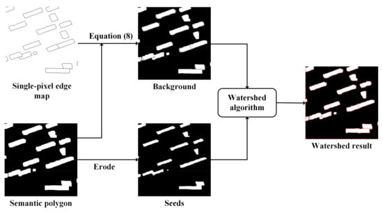
Figure 4.
Details of watershed algorithm. The single-pixel edge and semantic polygon use Equation (8) to generate background. The semantic polygon is eroded to generate seeds for the watershed algorithm. The watershed algorithm uses seeds to extract the correct edge (red line in watershed result) in the background.
In the second case, the semantic polygon object and single-pixel edge are fused by Equation (9), which can highlight the edge information outside the semantic polygon. (as shown in Figure 3e), after filling the holes, a complete semantic polygon (as shown in Figure 3f) can be obtained. At this time, the boundary of the obtained semantic polygon results becomes more regular and fits the real building boundary.
Finally, we solve the problem that adjacent buildings cannot be distinguished in semantic segmentation. The eight-neighborhood algorithm is used to determine whether the edge is the boundary of adjacent buildings and obtain the result of precise semantic segmentation of buildings (as shown in Figure 3h). This operation overcomes the above problems by fusing accurate edge information, and the accurate edge of the building (as shown in Figure 3g) is obtained.
More importantly, through the series of operations mentioned above, the integrity of the semantic polygon is used to repair the broken line in the single-pixel edge map, and the details of repairing a broken line are shown in Figure 5. If the boundary of the semantic polygon cannot realize the connection of the broken line, the broken line will be removed, and the boundary of the semantic polygon will be retained. The final edge result is guaranteed to be complete.
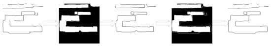
Figure 5.
Details of repairing a broken line.
In the postprocessing stage, by fusing the accurate edge information with the accurate semantic segmentation information, our method can make the positioning of high-level prediction more accurate. More importantly, the edge and segmentation details become better, especially the edge of buildings, which cannot be recognized by semantic segmentation, and the problem of broken lines in edge detection.
3. Results
3.1. Dataset
We choose two high-resolution remote-sensing image areas of representative buildings as our experimental area to evaluate our method on different datasets. Moreover, one is from Google images, and the other is aerial images.
- (1)
- The first is Beijing, the capital of China. The Beijing scene represents a typical Chinese urban landscape, including different types of buildings, which are difficult to accurately discriminate and extract. We selected four districts in the center of Beijing. The original Google images with a spatial resolution of 0.536 m are Chaoyang District, Haidian District, Dongcheng District, and Xicheng District.
- (2)
- The second is Zhonglu countryside, located in Weixi County, Diqing Prefecture, Yunnan Province. As a typical representative of rural architecture, its buildings have a relatively regular and uniform building shape. The original aerial images with a spatial resolution of 0.075 m.
We select samples with typical architectural features and a certain number of negative samples that do not contain buildings in the abovementioned study area, draw the precise boundary of the building manually, generate corresponding line labels and polygon labels, and randomize divide 80% of the samples are used as the training set, and 20% of the samples are used as the test set. The Beijing area contains 320 training sets of 512 pixel × 512-pixel images and 80 test sets of 512 pixel × 512-pixel images. The Zhonglu area contains 75 training sets of 1024 pixel × 1024-pixel images and 23 test sets of 1024 pixel × 1024-pixel images. The data set is shown in Figure 6.
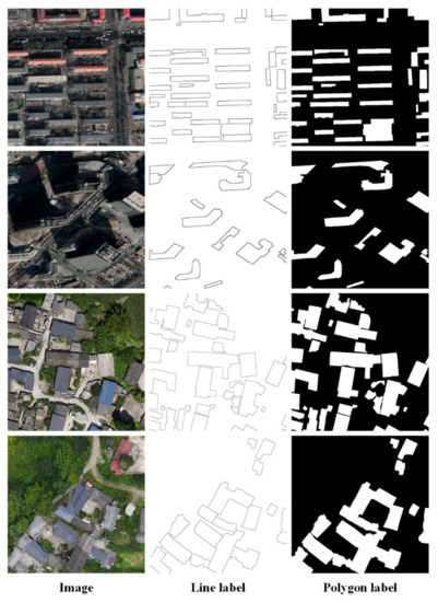
Figure 6.
Dataset display. Image represents high-resolution remote-sensing image, line label and polygon label are ground truth of the image, the first two are Beijing dataset, the last two are Zhonglu dataset.
3.2. Training Details
In our experiments, all deep learning network models are implemented using the PyTorch framework. DDLNet and the comparative experiments are all trained on an NVIDIA RTX TITAN (with 24 G memory) graphics card. We initialize the weights of the DDLNet with the weights of a ResNet34 model pretrained via ImageNet [35]. Some hyperparameters are set as follows: The batchsize on Beijing dataset and Zhonglu dataset are 4 and 2, respectively. The initial learning rate of DDLNet is 2 × 10⁻⁴, and the learning rate is updated for 1/4 of the total epochs. We trained 800 epochs on Beijing dataset and 400 epochs on Zhonglu dataset with DDLNet. Due to the insufficient amount of data, we adopt a data enhancement operation including random cropping, rotation, translation, and horizontal flipping operations after entering the network to expand the dataset and reduce overfitting.
3.3. Evaluation Metrics
We use Intersection over Union (IoU) and F1 score to evaluate the performance of our method. The IoU index represents the overlap ratio between the predicted area and the real area of an image. The higher the overlap rate is, the higher the accuracy of the predicted results. Equation (10) is as follows: represents the prediction area, and represents the real label area:
However, IoU can only evaluate the prediction accuracy of the building polygon result but cannot reflect the prediction accuracy of the building boundary. Therefore, we propose the boundary IoU method to evaluate the accuracy between the predicted building edge and the real building boundary. This method expands the edge by kernel size = 5 pixels and then uses Equation (11) to calculate the accuracy. Exp represents expand and represents kernel size:
Polygon IoU can reflect the completeness of the edge, and boundary IoU can reflect the accuracy of the polygon boundary.
The F1 score is an index used to measure the accuracy of a two-category model. To calculate the F1 score, it is necessary to calculate the precision and recall. In the following formulas, true positives (TP) represent the number of positive pixels belonging to buildings that are correctly identified. True negatives (TN) represent the number of negative pixels belonging to nonbuildings that are correctly identified. False positives (FP) represent the number of negative pixels belonging to nonbuildings that are incorrectly identified as positive pixels belonging to buildings. False negatives (FN) represent the number of positive pixels belonging to buildings that are incorrectly identified as negative pixels belonging to nonbuildings. The explanation of the above TP, TN, FP, FN indicators is shown in Figure 7.
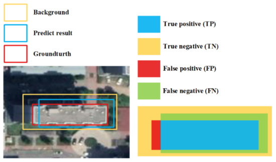
Figure 7.
Graphic representation of the TP, TN, FP, FN for the matched ground truth and predicted result.
Precision is the ratio of true positives in the identified positive pixels, and Equation (12) is as follows.
Recall is the proportion of all positive pixels in the test set that are correctly identified as positive pixels, and Equation (13) is as follows.
The F1 score is the harmonic mean value of the precision rate and recall rate, which suggests that the precision rate and recall rate are equally important. The larger the value, the stronger the model’s ability, and Equation (14) is as follows.
3.4. Results
To further demonstrate the effectiveness of our methods, we select some soft-of-the-art models to compare with our model and the postprocessing method.
First, for semantic edge detection, to assess the quality of our DDLNet model, three models, namely RCF, BDCN, and DexiNed, were selected for comparison with DDLNet on the Beijing and Zhonglu datasets.
In the Beijing dataset, RCF, BDCN and DexiNed achieved boundary IoU of 0.2815, 0.4087 and 0.4503, respectively. DDLNet achieved a boundary IoU of 0.5116, which greatly surpasses the accuracy of the other models. As shown in Table 1, RCF, BDCN, and DexiNed achieved polygon IoU of 0.2751, 0.5110 and 0.1724, respectively. DDLNet achieved a polygon IoU of 0.5295, which is 3.62% more than that of BDCN. The results of those semantic edge detection models on the Beijing test dataset are summarized in Table 1, and their performance are shown in Figure 8.

Table 1.
The results of semantic edge detection on the Beijing dataset.
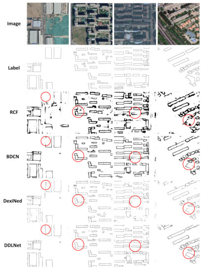
Figure 8.
The edge results of RCF, BDCN, DexiNed, and DDLNet on the Beijing dataset.
In the Zhonglu dataset, RCF, BDCN, DexiNed, DDLNet achieved boundary IoU values of 0.4378, 0.7050, 0.6326 and 0.7399 and achieved polygon IoU values of 0.5824, 0.7009, 0.6452 and 0.8719, respectively. The results of those semantic edge detection models on the Zhonglu test dataset are summarized in Table 2, and their performances are shown in Figure 9.
Table 2.
The results of semantic edge detection on the Zhonglu dataset.
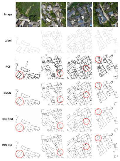
Figure 9.
The edge results of RCF, BDCN, DexiNed, and DDLNet on the Zhonglu dataset.
The capability of DDLNet for semantic edge detection tasks is demonstrated on two different data sets. RCF does not perform well on our dataset. BDCN can effectively extract the building boundary and ensure the integrity of the boundary, but its edge is blurred and insufficient in accuracy. DexiNed can produce more accurate and visual edges, but its edge integrity is difficult to guarantee. DDLNet can achieve edge integrity beyond DexiNed and BDCN and effectively extract the boundaries of buildings. It means that it is effective to provide more high-level semantic features for low-level edge features to realize semantic edge extraction.
Second, for semantic segmentation, we also selected three advanced models, namely U-Net, U-Net3+, and D-LinkNet, for the experiment on the Beijing and Zhonglu datasets.
In the Beijing dataset, U-Net, U-Net3+, and D-LinkNet achieved 0.6726, 0.7161, and 0.7212 in polygon IoU, respectively. DDLNet achieved the top performance of 0.7527 of the polygon IoU, which was better than all other models, and even 4.36% more than D-LinkNet. U-Net3+ and DDLNet use the full-scale skip connection to help network learning, and they achieved boundary IoU of 0.4731 and 0.4746, respectively. This greatly surpassed the accuracy of U-Net and D-LinkNet, which achieve boundary IoU of 0.4281 and 0.4438, respectively. The results of those semantic segmentation models on the Beijing test dataset are summarized in Table 3, and their performances are shown in Figure 10.
Table 3.
The results of semantic segmentation on the Beijing dataset.
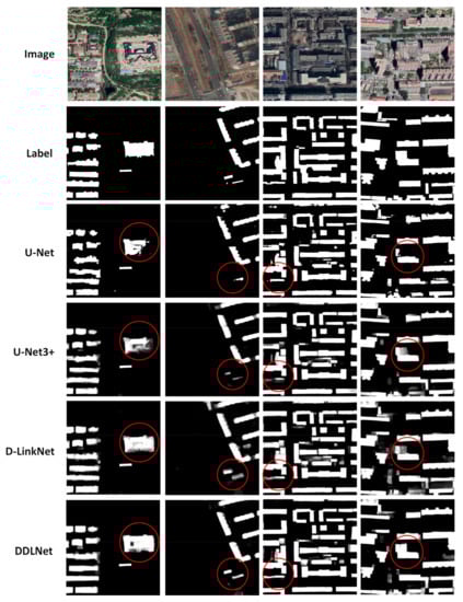
Figure 10.
The semantic polygon results of U-Net, U-Net3+, D-LinkNet, and DDLNet on the Beijing dataset.
In the Zhonglu dataset, U-Net, Unet3+, and D-LinkNet achieved 0.7067, 0.8855, and 0.9261 in polygon IoU, respectively. DDLNet achieved the best performance of 0.9364 of the polygon IoU. U-Net3+ and DDLNet achieve boundary IoU of 0.5396 and 0.6905 which greatly surpassed the accuracy of U-Net and D-LinkNet. The results of those semantic segmentation models on the Zhonglu test dataset are summarized in Table 4, and their performances are shown in Figure 11.
Table 4.
The results of semantic segmentation on the Zhonglu dataset.
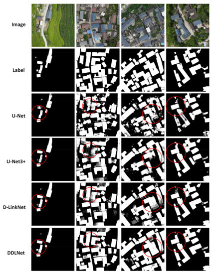
Figure 11.
The semantic polygon results of U-Net, U-Net3+, D-Linknet, and DDLNet on the Zhonglu dataset.
The capability of DDLNet for semantic segmentation tasks is demonstrated on two different data sets. U-Net3+ and DDLNet achieve boundary IoU greatly surpassed the accuracy of U-Net and D-LinkNet that proves that the full-scale skip connection is effective in improving the boundary of the polygon from semantic segmentation. The result of DDLNet proves that making full use of low-level edge information proved to be helpful in extracting buildings from high-resolution remote sense images.
Moreover, we evaluated the effectiveness of the postprocessing method. We choose a variety of semantic edge models and semantic segmentation models to verify the effectiveness of our postprocessing scheme. The criteria we chose were that the boundary IoU of the semantic edge model was larger than that of the semantic segmentation model to improve the edge accuracy of the semantic polygon, and the polygon IoU of the semantic segmentation model was larger than that of the semantic edge model to improve the integrity of the semantic edge.
Based on the criteria, in the Beijing test dataset, we choose DDLNet combined with DDLNet, D-LinkNet, U-Net3+, and U-Net. DexiNed combined with D-LinkNet and U-Net. Compared with Table 1 and Table 3, the results of postprocessing improve the polygon IoU of semantic edge detection and the boundary IoU of semantic segmentation. In addition, the results are closer to manual vision. The combination and the results of the combination are shown in Table 5 and Figure 12.
Table 5.
The results of the postprocessing method on the Beijing dataset.
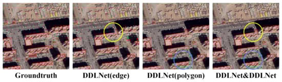
Figure 12.
The results of postprocessing method with DDLNet on the Beijing dataset. DDLNet (edge) represent the edge result of DDLNet. In addition, DDLNet (polygon) represent the polygon result of DDLNet. DDLNet&DDLNet represent the result of postprocessing method. The blue circle mark shows the improvement of semantic segmentation where the boundary is closer to the real boundary of building, and the yellow circle mark shows the improvement of semantic edge where the disconnection edge was repaired completely.
Based on the criteria, in the Zhonglu test dataset, we choose DDLNet combined with DDLNet, D-LinkNet, U-Net3+, and U-Net. BDCN combined with DDLNet, D-LinkNet, U-Net3+, U-Net. DexiNed combined with D-LinkNet and U-Net. RCF combined with U-Net. Compared with Table 2 and Table 4, the results of postprocessing improve the polygon IoU of semantic edge detection and the boundary IoU of semantic segmentation. The combination and the results of the combination are shown in Table 6 and Figure 13.
Table 6.
The results of the postprocessing method on the Zhonglu dataset.
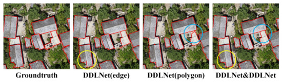
Figure 13.
The results of postprocessing method with DDLNet on the Zhonglu dataset. DDLNet (edge) represent the edge result of DDLNet. In addition, DDLNet (polygon) represent the polygon result of DDLNet. DDLNet&DDLNet represent the result of postprocessing method. The blue circle mark shows the improvement of semantic segmentation where the boundary is closer to the real boundary of building, and the yellow circle mark shows the improvement of semantic edge where the disconnection edge was repaired completely.
In summary, we conducted comparative experiments on two different datasets with other SOTA models to verify whether our methods could obtain high-quality results. Experiments confirmed that our model DDLNet had better results than other SOTA models in both semantic edge detection tasks and semantic segmentation tasks and all evaluation metrics, which not only indicated that our models have a good performance in building extraction but also indicates that the edge guidance module and full-scale skip connection are conducive to the automatic extraction of buildings in a network. What’s more, our postprocessing method is effective and further improved results of building extraction that helps to improve the vectorization of the result.
4. Discussion
There are certain shortcomings of neural network-based deep learning methods. The edge detection network usually adopts a multiscale fusion strategy to preserve more detailed predictions, resulting in fuzzy and insufficient refinement of the final edge results, as well as difficulty in solving edge disconnection problems. From the experiments and results in the fourth section, DDLNet has better detection accuracy and visual effects than the other edge detection models. The decoder combines the semantic information of the previous layer and the edge information of this layer to improve the accuracy. Through the especially designed CMSE loss, the problem of edge blur, roughness and disconnection is reduced to a certain extent. However, the current loss function design still has problems, and the final edge result still has a disconnection problem.
For the semantic segmentation task, which focuses on the pixel-level classification of targets, the previous semantic segmentation network structure focuses more on the contextual and semantic information of the targets, ignoring the importance of edge information, which leads to difficulty in matching the boundaries of the final semantic polygons with the boundaries of real buildings. Compared with the current semantic segmentation, DDLNet has been improved to a certain extent. From the boundary IoU indicator, we find that the full-scale skip connection and edge guidance module are simple and effective to improve the boundary of buildings.
Convolutional neural networks adopt downsampling pooling operations in encoder and upsampling operations in decoder, and the use of downsampling to compress data is irreversible, resulting in information loss and therefore causing translation invariance and poor results [4]. The loss of information is irreversible, so we design a method to fuse the edge information and semantic information from a postprocessing perspective to achieve precise building extraction. The experimental results show the effectiveness of our postprocessing method, and the final result shows both the edge precision of edge detection and the semantic precision of semantic segmentation. After postprocessing, the boundary IoU and polygon IoU of most final results have improved.
However, some results provide lower-boundary IoU compared with the initial single edge detection in Table 5. As we consider, while the polygon cannot realize the supplement of the disconnection line, we will remove the disconnection line and choose the polygon boundary. Moreover, the polygon may lead to a false detection polygon in the final result. Considering that the polygon boundary may be poor, the final result may have a lower-boundary IoU. At the same time, the hyperparameter setting of the watershed algorithm will also influence the result. This means that the postprocessing process can be further improved.
5. Conclusions
This article focuses on solving the problem of edge discontinuity and incompleteness generated by semantic edge detection, and the polygon shape generated by semantic segmentation is irregular, which does not match the actual building boundary. We propose a novel CNN model named Dense D-LinkNet (DDLNet). DDLNet uses full-scale skip connection, deep multiscale supervision and edge guidance module to overcome the aforementioned problem. The experimental results show that DDLNet is useful and has a certain degree of improvement in the evaluation indicator boundary IoU and polygon IoU in both semantic edge detection tasks and semantic segmentation tasks. Moreover, our postprocessing method is effective and universal and can arbitrarily fuse semantic edge information from edge detection with semantic polygons from semantic segmentation to improve the quality of the final result of buildings.
Author Contributions
L.X. and J.Z. designed and completed the experiments and wrote the article. X.Z., H.Y. and M.X. guided this process and helped with the writing of the paper. All authors have read and agreed to the published version of the manuscript.
Funding
This work was supported in part by the National Key Research and Development Program of China under Grants 2018YFB0505300 and 2017YFB0503600, in part by the National Natural Science Foundation of China under Grant 41701472, in part by the Zhejiang Provincial Natural Science Foundation of China under Grant No. LQ19D010006.
Institutional Review Board Statement
Not applicable.
Informed Consent Statement
Not applicable.
Data Availability Statement
The code of DDLNet is publicly available at https://github.com/Pikachu-zzZ/DDLNet (accessed on 20 June 2021).
Acknowledgments
We would like to acknowledge the Landthink in Suzhou for supporting the Google Earth data and aerial image data.
Conflicts of Interest
No potential conflict of interest was reported by the authors.
References
- Gilani, S.A.N.; Awrangjeb, M.; Lu, G. Segmentation of airborne point cloud data for automatic building roof extraction. GISci. Remote Sens. 2018, 55, 63–89. [Google Scholar] [CrossRef] [Green Version]
- Lu, T.; Ming, D.; Lin, X.; Hong, Z.; Bai, X.; Fang, J. Detecting building edges from high spatial resolution remote sensing imagery using richer convolution features network. Remote Sens. 2018, 10, 1496. [Google Scholar] [CrossRef] [Green Version]
- Hung, C.-L.J.; James, L.A.; Hodgson, M.E. An automated algorithm for mapping building impervious areas from airborne LiDAR point-cloud data for flood hydrology. GISci. Remote Sens. 2018, 55, 793–816. [Google Scholar] [CrossRef]
- Yang, G.; Zhang, Q.; Zhang, G. EANet: Edge-aware network for the extraction of buildings from aerial images. Remote Sens. 2020, 12, 2161. [Google Scholar] [CrossRef]
- Bischke, B.; Helber, P.; Folz, J.; Borth, D.; Dengel, A. Multi-task learning for segmentation of building footprints with deep neural networks. In Proceedings of the 2019 IEEE International Conference on Image Processing (ICIP), Taipei, Taiwan, 22–25 September 2019; pp. 1480–1484. [Google Scholar]
- Yang, H.; Yu, B.; Luo, J.; Chen, F. Semantic segmentation of high spatial resolution images with deep neural networks. GISci. Remote Sens. 2019, 56, 749–768. [Google Scholar] [CrossRef]
- Yi, Y.; Zhang, Z.; Zhang, W.; Zhang, C.; Li, W.; Zhao, T. Semantic segmentation of urban buildings from vhr remote sensing imagery using a deep convolutional neural network. Remote Sens. 2019, 11, 1774. [Google Scholar] [CrossRef] [Green Version]
- Huang, H.; Sun, G.; Rong, J.; Zhang, A.; Ma, P. Multi-feature Combined for Building Shadow detection in GF-2 Images. In Proceedings of the 2018 Fifth International Workshop on Earth Observation and Remote Sensing Applications (EORSA), Xi’an, China, 18–20 June 2018; pp. 1–4. [Google Scholar]
- Ji, S.; Wei, S.; Lu, M. Fully convolutional networks for multisource building extraction from an open aerial and satellite imagery data set. IEEE Trans. Geosci. 2018, 57, 574–586. [Google Scholar] [CrossRef]
- Xie, S.; Tu, Z. Holistically-nested edge detection. In Proceedings of the IEEE International Conference on Computer Vision, Santiago, Chile, 7–13 December 2015; pp. 1395–1403. [Google Scholar]
- Liu, Y.; Cheng, M.-M.; Hu, X.; Wang, K.; Bai, X. Richer convolutional features for edge detection. In Proceedings of the IEEE Conference on Computer Vision and Pattern Recognition, Honolulu, HI, USA, 21–26 July 2017; pp. 3000–3009. [Google Scholar]
- He, J.; Zhang, S.; Yang, M.; Shan, Y.; Huang, T. Bi-directional cascade network for perceptual edge detection. In Proceedings of the IEEE Conference on Computer Vision and Pattern Recognition, Long Beach, CA, USA, 15–20 June 2019; pp. 3828–3837. [Google Scholar]
- Hu, Y.; Chen, Y.; Li, X.; Feng, J. Dynamic feature fusion for semantic edge detection. arXiv 2019, arXiv:1902.09104. [Google Scholar]
- Yu, Z.; Feng, C.; Liu, M.-Y.; Ramalingam, S. Casenet: Deep category-aware semantic edge detection. In Proceedings of the IEEE Conference on Computer Vision and Pattern Recognition, Honolulu, HI, USA, 21–26 July 2017; pp. 5964–5973. [Google Scholar]
- He, K.; Zhang, X.; Ren, S.; Sun, J. Deep residual learning for image recognition. In Proceedings of the IEEE Conference on Computer Vision and Pattern Recognition, Las Vegas, NV, USA, 27–30 June 2016; pp. 770–778. [Google Scholar]
- Reda, K.; Kedzierski, M. Detection, Classification and Boundary Regularization of Buildings in Satellite Imagery Using Faster Edge Region Convolutional Neural Networks. Remote Sens. 2020, 12, 2240. [Google Scholar] [CrossRef]
- He, K.; Zhang, X.; Ren, S.; Sun, J. Delving deep into rectifiers: Surpassing human-level performance on imagenet classification. In Proceedings of the IEEE International Conference on Computer Vision, Santiago, Chile, 7–13 December 2015; pp. 1026–1034. [Google Scholar]
- Long, J.; Shelhamer, E.; Darrell, T. Fully convolutional networks for semantic segmentation. In Proceedings of the IEEE Conference on Computer Vision and Pattern Recognition, Boston, MA, USA, 8–10 June 2015; pp. 3431–3440. [Google Scholar]
- Ronneberger, O.; Fischer, P.; Brox, T. U-net: Convolutional networks for biomedical image segmentation. In Proceedings of the International Conference on Medical Image Computing and Computer-Assisted Intervention, Munich, Germany, 5–9 October 2015; pp. 234–241. [Google Scholar]
- Badrinarayanan, V.; Kendall, A.; Cipolla, R. Segnet: A deep convolutional encoder-decoder architecture for image segmentation. IEEE Trans. Pattern Anal. Mach. Intell. 2017, 39, 2481–2495. [Google Scholar] [CrossRef] [PubMed]
- Lin, G.; Milan, A.; Shen, C.; Reid, I. Refinenet: Multi-path refinement networks for high-resolution semantic segmentation. In Proceedings of the IEEE Conference on Computer Vision and Pattern Recognition, Honolulu, HI, USA, 21–26 July 2017; pp. 1925–1934. [Google Scholar]
- Zhao, H.; Shi, J.; Qi, X.; Wang, X.; Jia, J. Pyramid scene parsing network. In Proceedings of the IEEE Conference on Computer Vision and Pattern Recognition, Honolulu, HI, USA, 21–26 July 2017; pp. 2881–2890. [Google Scholar]
- Liu, P.; Liu, X.; Liu, M.; Shi, Q.; Yang, J.; Xu, X.; Zhang, Y. Building footprint extraction from high-resolution images via spatial residual inception convolutional neural network. Remote Sens. 2019, 11, 830. [Google Scholar] [CrossRef] [Green Version]
- Delassus, R.; Giot, R. CNNs Fusion for Building Detection in Aerial Images for the Building Detection Challenge. In Proceedings of the CVPR Workshops, Salt Lake City, UT, USA, 18–22 June 2018; pp. 242–246. [Google Scholar]
- Lin, J.; Jing, W.; Song, H.; Chen, G. ESFNet: Efficient network for building extraction from high-resolution aerial images. IEEE Access 2019, 7, 54285–54294. [Google Scholar] [CrossRef]
- Wang, S.; Zhou, L.; He, P.; Quan, D.; Zhao, Q.; Liang, X.; Hou, B. An Improved Fully Convolutional Network for Learning Rich Building Features. In Proceedings of the IGARSS 2019–2019 IEEE International Geoscience and Remote Sensing Symposium, Yokohama, Japan, 28 July–2 August 2019; pp. 6444–6447. [Google Scholar]
- Batra, A.; Singh, S.; Pang, G.; Basu, S.; Jawahar, C.; Paluri, M. Improved road connectivity by joint learning of orientation and segmentation. In Proceedings of the IEEE/CVF Conference on Computer Vision and Pattern Recognition, 15–20 June 2019; pp. 10385–10393. [Google Scholar]
- Zhang, Y.; Yang, Q. A survey on multi-task learning. IEEE Trans. Knowl. Data Eng. 2021. [Google Scholar] [CrossRef]
- Zhou, L.; Zhang, C.; Wu, M. D-LinkNet: LinkNet With Pretrained Encoder and Dilated Convolution for High Resolution Satellite Imagery Road Extraction. In Proceedings of the CVPR Workshops, Salt Lake City, UT, USA, 18–22 June 2018; pp. 182–186. [Google Scholar]
- Chaurasia, A.; Culurciello, E. Linknet: Exploiting encoder representations for efficient semantic segmentation. In Proceedings of the 2017 IEEE Visual Communications and Image Processing (VCIP), Saint Petersburg, FL, USA, 10–13 December 2017; pp. 1–4. [Google Scholar]
- Huang, G.; Liu, Z.; Van Der Maaten, L.; Weinberger, K.Q. Densely connected convolutional networks. In Proceedings of the IEEE Conference on Computer Vision and Pattern Recognition, Honolulu, HI, USA, 21–26 July 2017; pp. 4700–4708. [Google Scholar]
- Huang, H.; Lin, L.; Tong, R.; Hu, H.; Zhang, Q.; Iwamoto, Y.; Han, X.; Chen, Y.-W.; Wu, J. Unet 3+: A full-scale connected unet for medical image segmentation. In Proceedings of the ICASSP 2020–2020 IEEE International Conference on Acoustics, Speech and Signal Processing (ICASSP), Virtual Conference, Barcelona, Spain, 4–8 May 2020; pp. 1055–1059. [Google Scholar]
- He, C.; Li, S.; Xiong, D.; Fang, P.; Liao, M. Remote Sensing Image Semantic Segmentation Based on Edge Information Guidance. Remote Sens. 2020, 12, 1501. [Google Scholar] [CrossRef]
- Vincent, L.; Soille, P. Watersheds in digital spaces: An efficient algorithm based on immersion simulations. IEEE Trans. Pattern Anal. Mach. Intell. 1991, 13, 583–598. [Google Scholar] [CrossRef] [Green Version]
- Deng, J.; Dong, W.; Socher, R.; Li, L.-J.; Li, K.; Fei-Fei, L. Imagenet: A large-scale hierarchical image database. In Proceedings of the 2009 IEEE Conference on Computer Vision and Pattern Recognition, Miami, FL, USA, 20–25 June 2009; pp. 248–255. [Google Scholar]
Publisher’s Note: MDPI stays neutral with regard to jurisdictional claims in published maps and institutional affiliations. |
© 2021 by the authors. Licensee MDPI, Basel, Switzerland. This article is an open access article distributed under the terms and conditions of the Creative Commons Attribution (CC BY) license (https://creativecommons.org/licenses/by/4.0/).