Article

Phytoplankton Bloom Dynamics in the Baltic Sea Using a Consistently Reprocessed Time Series of Multi-Sensor Reflectance and Novel Chlorophyll-a Retrievals

1
Consiglio Nazionale delle Ricerche, Istituto di Scienze Marine (CNR-ISMAR), 00133 Rome, Italy
2
Aequora, 1600-774 Lisbon, Portugal
3
Finnish Environment Institute (SYKE), 00790 Helsinki, Finland
*
Author to whom correspondence should be addressed.
Remote Sens. 2021, 13(16), 3071; https://doi.org/10.3390/rs13163071
Submission received: 5 July 2021 / Revised: 20 July 2021 / Accepted: 21 July 2021 / Published: 4 August 2021
(This article belongs to the Special Issue Baltic Sea Remote Sensing)

Abstract

:
A relevant indicator for the eutrophication status in the Baltic Sea is the Chlorophyll-a concentration (Chl-a). Alas, ocean color remote sensing applications to estimate Chl-a in this brackish basin, characterized by large gradients in salinity and dissolved organic matter, are hampered by its optical complexity and atmospheric correction limits. This study presents Chl-a retrieval improvements for a fully reprocessed multi-sensor time series of remote-sensing reflectances (Rrs) at ~1 km spatial resolution for the Baltic Sea. A new ensemble scheme based on multilayer perceptron neural net (MLP) bio-optical algorithms has been implemented to this end. The study documents that this approach outperforms band-ratio algorithms when compared to in situ datasets, reducing the gross overestimates of Chl-a observed in the literature for this basin. The Rrs and Chl-a time series were then exploited for eutrophication monitoring, providing a quantitative description of spring and summer phytoplankton blooms in the Baltic Sea over 1998–2019. The analysis of the phytoplankton dynamics enabled the identification of the latitudinal variations in the spring bloom phenology across the basin, the early blooming in spring in the last two decades, and the description of the spatiotemporal coverage of summer cyanobacterial blooms in the central and southern Baltic Sea.

Graphical Abstract

1. Introduction

The status of eutrophication in the Baltic Sea has been a constant concern [1,2,3,4,5]. The Baltic Sea Action Plan [3] by the Baltic Marine Environment Protection Commission (Helsinki Commission, HELCOM) presents actions to improve the sea condition. One of the indicators relevant to the eutrophication assessment is the Chlorophyll-a concentration ( C h l - a ), based on a combination of data from station sampling, automated ship measurements, and remote sensing [4,6,7]. As an example of Baltic Sea countries, Finland already utilizes remote sensing C h l - a in its national monitoring program, along with some other water quality parameters [8]. Although Earth Observation programs have significantly improved the retrieval of ocean color (OC) data products on a global scale [9,10,11,12,13], the quality of regional results, and more specifically OC product maps in optically complex waters such as the Baltic Sea, still challenge remote sensing capabilities [13,14,15]. The case study addressed in this work is the improved C h l - a determination based on regional bio-optical algorithms in view of supporting the environmental assessment of the basin.
The Baltic Sea (Figure 1) is a brackish shallow enclosed basin, characterized by large gradients in salinity and dissolved organic matter, where algal blooms are strongly related to anoxia and hypoxia events [5,16,17,18]. Seasonal changes in phytoplankton composition and the occurrence of extensive phytoplankton surface blooms in this basin depend on various drivers, including nutrient inputs from natural and human sources, salinity, ice coverage, and temperature stratification in the water column [16,19]. The dominant phytoplankton group of spring blooms is usually associated with diatoms and then dinoflagellates [19,20,21], while the summer months are characterized by extensive surface or near-surface blooms dominated by nitrogen-fixing cyanobacteria, particularly in July and August [20,22,23].
The C h l - a retrieval in the Baltic Sea is hampered by two complementary difficulties [24,25,26,27]. The first is the optical complexity of the basin, where the colored dissolved organic matter (CDOM) dominates the absorption budget in the blue spectral range with a high variability over short spatial scales, leading to low reflectance especially in the blue part of the spectrum [20,27,28,29,30,31]. The second is the reduced performance of the atmospheric correction, often producing erroneously low or even negative R r s values, consequently limiting the capability to retrieve accurate R r s spectral images [24,27,32,33,34]. As a result, standard algorithms based on a blue–green band-ratio polynomial regression developed for SeaWIFS (Sea-viewing Wide-Field-of-view Sensor) and MODIS (Moderate Resolution Imaging Spectroradiometer) tend to largely overestimate C h l - a in the basin [25,26,27,35,36,37].
Based on a series of radiative transfer simulations aimed at representing the bio-optical characteristics of the Baltic Sea, including the seasonal variability in phytoplankton dominance [20], Ligi et al. [26] tested several global and regional C h l - a algorithms. Their results showed that the band-ratio algorithms that use R r s values in the blue-green spectral regions were inaccurate due to the water optical complexity, confirming the previous findings by several authors (e.g., [24,25]). However, these studies also showed that band-ratio algorithms in the red and NIR spectral regions, mostly using MERIS (MEdium spectral Resolution Imaging Spectrometer) spectral bands, yielded high correlation on simulated data, but their performance produced at best a r2 of 0.4‒0.6 when tested on in situ data (e.g., [23,24,25]) for C h l - a in the range between ∼1 and 10 μgL−1 (i.e., at the lower part of the retrievable concentrations by these algorithms [37]). Neural Network algorithms relying on SeaWIFs, MERIS and OLCI (Ocean and Land Colour Instrument) band-sets were also tested but reported limited retrieval accuracy [24,38,39,40,41,42].
The need to enhance the accuracy of C h l - a maps in the Baltic Sea is recognized by international space programs, and specifically prioritized by the data products release undertaken by the Copernicus Marine Environment Monitoring Service (CMEMS) [43,44]. Two operational C h l - a data-streams are available in CMEMS for the Baltic Sea: a near real-time based on OLCI, and a fully reprocessed multi-sensor time series produced with consolidated and consistent input datasets [15].
Recent C h l - a retrieval improvements for the Baltic Sea multi-sensor time series are presented in this study. Based on the multilayer perceptron neural net (MLP) developed with the in situ data acquired in the study area [29,45], a new bio-optical ensemble scheme, named ENS-MLP, is conceived in the present work. Performance benchmarks with standard and regional band-ratio algorithms for the Baltic Sea are presented [11,36,46,47]. A core feature of the study is to use independent in situ measurements collected in the Baltic Sea for the analysis and assessment of results. Finally, the fully consistently reprocessed R r s and novel C h l - a time series (1998–2019) are analyzed to provide a quantitative description of the phytoplankton bloom dynamics for spring and summer seasons at basin and sub-basin scales.
The remainder of this document is organized as follows. Data and methods are presented in Section 2 by describing the space-borne R r s dataset, the MLP and ENS-MLP regional algorithms, the reference field measurements, and the indicators for spring and summer phytoplankton blooms in the basin. Section 3 accounts for (1) assessment of R r s and C h l - a estimates in reference to in situ measurements, and (2) occurrence of spring and summer blooms in the Baltic Sea over 1998–2019. Study remarks and conclusions are finally addressed in Section 4.

2. Materials and Methods

2.1. Space-Borne R r s

Space-borne radiometric observations include R r s at 412, 443, 490, 510, 555, and 670 nm collected over the Baltic Sea for more than twenty years (1997 to 2019). A consistent data processing scheme has been adopted to produce and release this time series. Namely, R r s spectra acquired by MERIS/ENVISAT, MODIS/AQUA, SeaWiFS/SEASTAR, and VIIRS/SUOMI-NPP space sensors were merged into a unique CMEMS dataset with 1 km resolution utilizing the processor Ver. 4.2 of the Ocean Color Climate Change Initiative (OC-CCI) [12].
Space-borne R r s values have been derived by applying atmospheric corrections specific to the processing of data from different sensors. The NASA standard atmospheric correction [48] was applied to MODIS, SeaWiFS, and VIIRS data (R2018.0 reprocessing) [49,50,51]. The POLYMER atmospheric correction [52] was instead adopted for MERIS (R2012.0 reprocessing). To account for the different sensor spectral resolutions, a band-shifting procedure based on the inverse and direct application of the QAA algorithm [53,54,55] was utilized to recompute results at the SeaWiFS bands [56]. Finally, in the multi-sensor merging scheme, the band-shifted R r s spectra from the available sensors have been individually bias-corrected with respect to a reference sensor mission [12,15]. Notable is the resulting enhanced product map coverage, which can be twice that of a single-sensor image when three different space missions are combined [53]. Thisincreased number of valid pixels is of utmost relevance to lessen the constraint of severe cloud cover in the Baltic Sea.

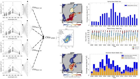
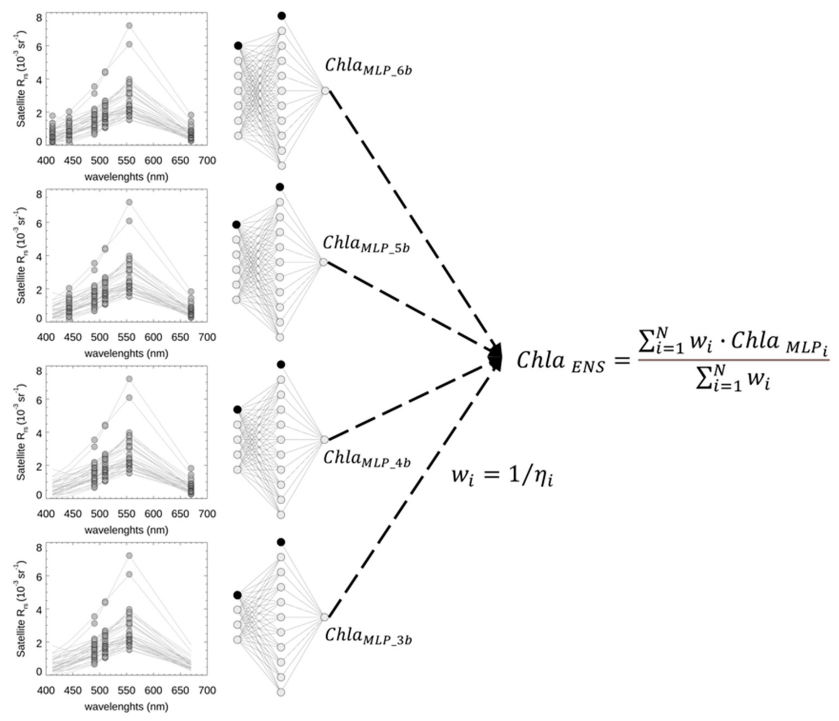
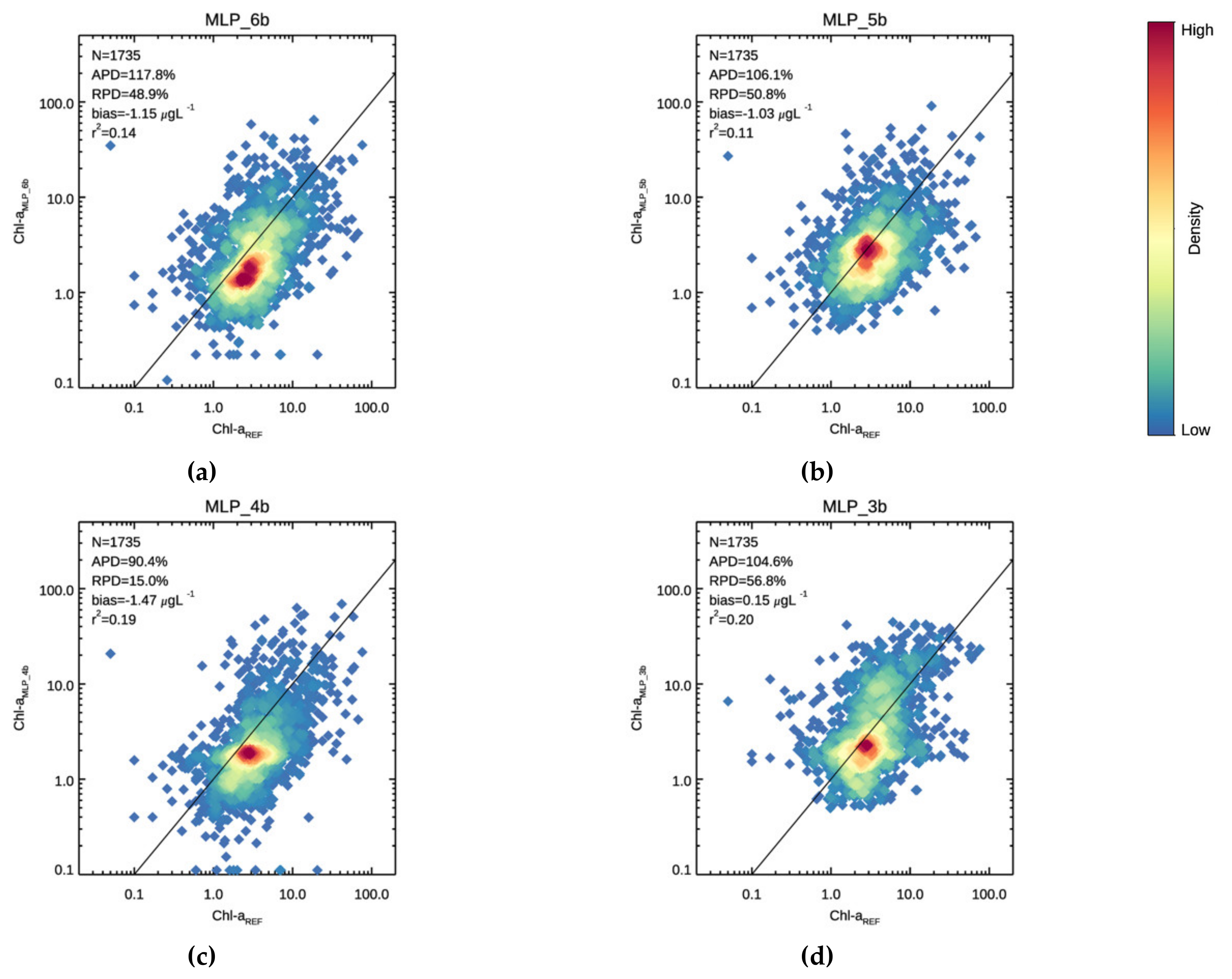
2.2. The Ensemble of MLP Bio-Optical Algorithms

The regional MLP of reference for deriving C h l - a estimates in the Baltic Sea was developed within the BiOMaP program of JRC/EC [29,45]. The MLP allows using R r s at individual wavelengths as input to compute C h l - a values. In this respect, the MLP can outperform band-ratio regression algorithms, which account for spectral R r s slopes rather than R r s values. However, the MLP suffers from poor extrapolation capabilities and its validity range needs to be supported by a novelty detection scheme to verify the statistical consistency between training data and R r s input spectra from which the C h l - a is operationally computed [57,58].
The validity range of MLPs based on different sets of input bands can also vary depending on the spectral heterogeneity of uncertainties induced by the atmospheric correction process on R r s values. Former analyses [57] have shown that R r s 670 is required to improve the C h l - a retrieval in the Baltic Sea, and that the best performance is achieved utilizing all six SeaWiFS bands. However, the same study has also identified a substantial reduction of the MLP performance when the set of input R r s is affected by spectral perturbations statistically consistent with those introduced by the atmospheric correction.
To address this performance degradation, an ensemble solution, inspired by the so-called “mixture of expert” approach in statistical pattern recognition [59,60], is proposed in the present work. Rather than adopting only a single MLP based on all CCI spectral bands (or a fixed subset of wavelengths), the idea is to rely on several MLPs using different R r s band-sets as input. Specifically, the C h l - a ensemble estimate ( C h l - a E N S ) is retrieved gathering individual MLPs that use different R r s spectral subsets by weighting their contribution through the corresponding novelty index (Figure 2). The sets of R r s bands evaluated in this work as MLP input are:
  • C h l - a M L P _ 6 b : 6 bands with R r s values at 412, 443, 490, 510, 555, and 670 nm.
  • C h l - a M L P _ 5 b : 5 bands with R r s values at 443, 490, 510, 555, and 670 nm.
  • C h l - a M L P _ 4 b : 4 bands with R r s values at 490, 510, 555, and 670 nm.
  • C h l - a M L P _ 3 b : 3 bands with R r s values at 490, 510, and 555 nm.
The new ensemble scheme proposed in this study combines different MLP results through a dynamical determination of the input bands’ relevance based on the novelty index. The mathematical expressions to implement the MLPs, to compute the novelty index, and to derive the ensemble C h l - a are reported next.

2.2.1. MLP Scheme

Based on previous analyses [57], the MLP architecture to retrieve C h l - a from input R r s has one hidden layer with ten neurons (see also Figure 2). The MLP algorithm development (a process referred to as MLP training) was based on 100 epochs using the Scaled Conjugate Gradient as a method for weights’ optimization and applying a weight decay regularization coefficient equal to 0.05. The numerical MLP implementation relied on the Netlab neural net toolbox for MATLAB [61,62]. The MLP performance with respect to the BiOMaP data was defined with three-fold cross-validation [29,45,57]. All available data were then used to train the operational input band-specific MLPs used in this study to target the highest Chl-a retrieval accuracy. All parameters to compute the C h l - a   M L P and the novelty index were determined with the BiOMaP measurements, building upon the approach detailed in [29,45,57] (see Supplementary Tables S1–S4). Computational steps including data pre- and post-processing as well as the definition of the MLP novelty index are summarized next.
Data pre-processing: Input R r s values are firstly log-transformed, l =   log 10 R r s , and then z-score scaled x = l μ l / σ l , where μ l and σ l indicate respectively the mean and standard deviation of log-transformed R r s values used for the MLP training.
Data regression: The MLP scheme consists of successive layers of units, with each unit in one layer connected to each unit of the next layer. Let y = f x denote the MLP function, where the input vector x has entries x i for i = 1 , , n λ , where n λ indicates the number of input R r s wavelengths. The value of the hidden unit j, denoted a j , is a linear combination of the input quantities:
a j = b j 1 + i = 1 n λ w j i 1 x i ,
where w j i 1 represents the weight linking the input unit i to the hidden unit j, and b j 1 is the bias adaptive parameter. The activation of the hidden unit j, identified with z j and representing the input for the next layer, is obtained as:
z j   =   g a j =   e a j e a j e a j + e a j ,
with g indicating the hyperbolic tangent activation function. The output y is computed as:
y = b 2 + i = 1 M w j 2 z j
where M indicates the number of hidden units with weight w j 2 , and b 2 is the bias coefficient.
Data post-processing: Data post-processing converts the y value computed by the MLP into the final data product as C h l - a = 10 y σ c + μ c , where μ c and σ c are respectively the mean and the standard deviation of log-transformed C h l - a values used for the MLP training.

2.2.2. Novelty Index and MLP Applicability Range

The MLP applicability range has been identified by means of the novelty index η [57,58], defined as follows:
ξ = l μ η   ·   A η
ζ = ξ   / γ η
η = ζ   / n λ
where l is the logarithm of the input R r s values, A η and γ η array are respectively the eigenvectors and eigenvalues from the principal component analysis (PCA) of the log-transformed R r s data used for MLP training, ‖ζ‖ is the Euclidean norm of ζ, and n λ is the number of selected R r s wavelengths.

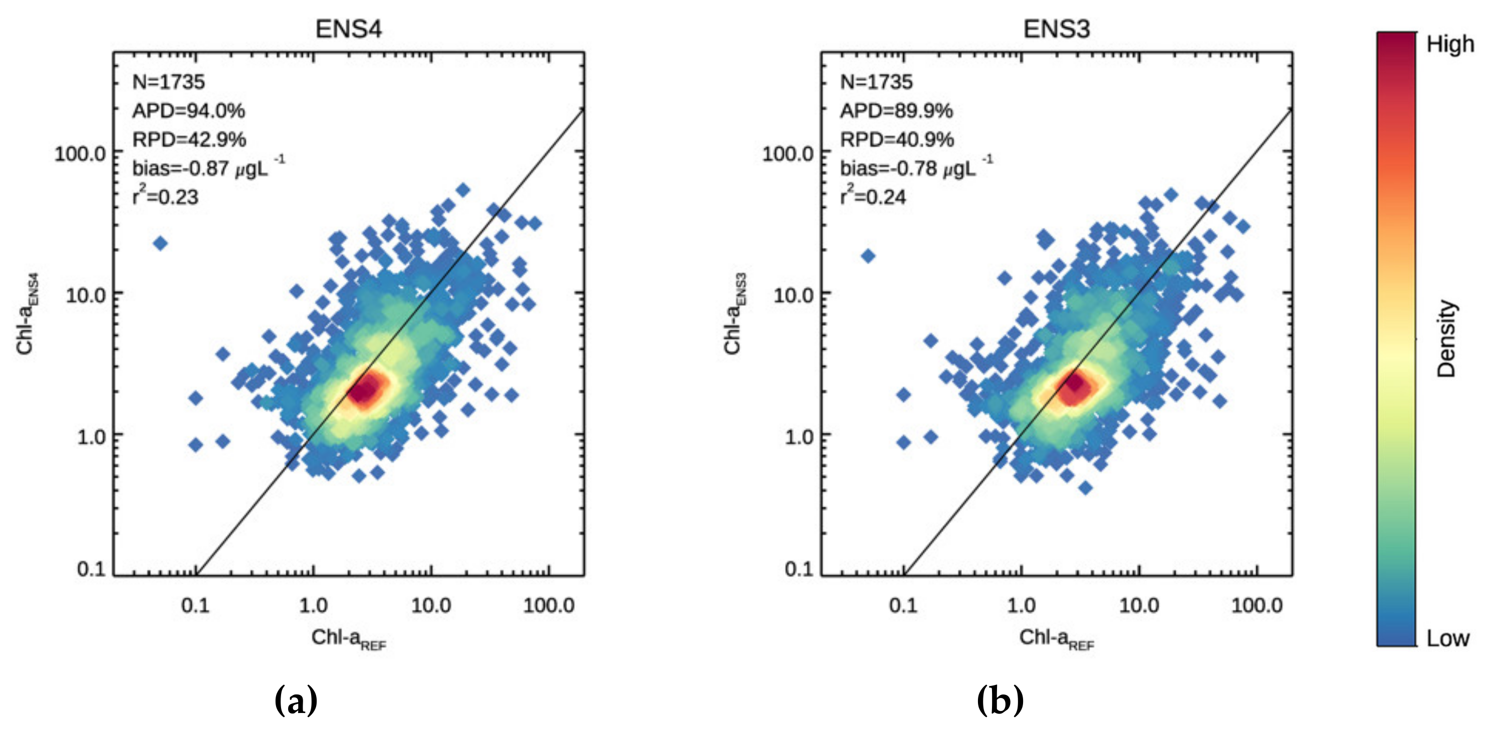
2.2.3. Ensemble Scheme

The ensemble scheme is described building on the equations reported above to derive C h l - a values with the MLP and determine the novelty index η (Figure 2). Namely, the MLP configuration that uses the i-th bands set is denoted as M L P i , and corresponding C h l - a   values and novelty index are indicated as C h l - a   M L P i and η i , respectively. A weight w i = 1 / η i is then assigned to C h l - a   M L P i to compute the ensemble result:
C h l - a   E N S = i = 1 N w i   ·   C h l - a   M L P i i = 1 N w i
To combine C h l - a estimates obtained with different MLPs based on R r s at specific wavelengths’ subsets, the weight definition is based on the assumption that the lower the novelty index η i , the more suitable the computed C h l - a   M L P i value [57,58]. Among the possible MLP ensemble configurations, this study will focus on the performance of the ensemble solutions based on four MLPs ( C h l - a E N S 4 : C h l - a M L P _ 6 b , C h l - a M L P _ 5 b , C h l - a M L P _ 4 b , C h l - a M L P _ 3 b ) and on three MLPs ( C h l - a E N S 3 : C h l - a M L P _ 5 b , C h l - a M L P _ 4 b , C h l - a M L P _ 3 b ).

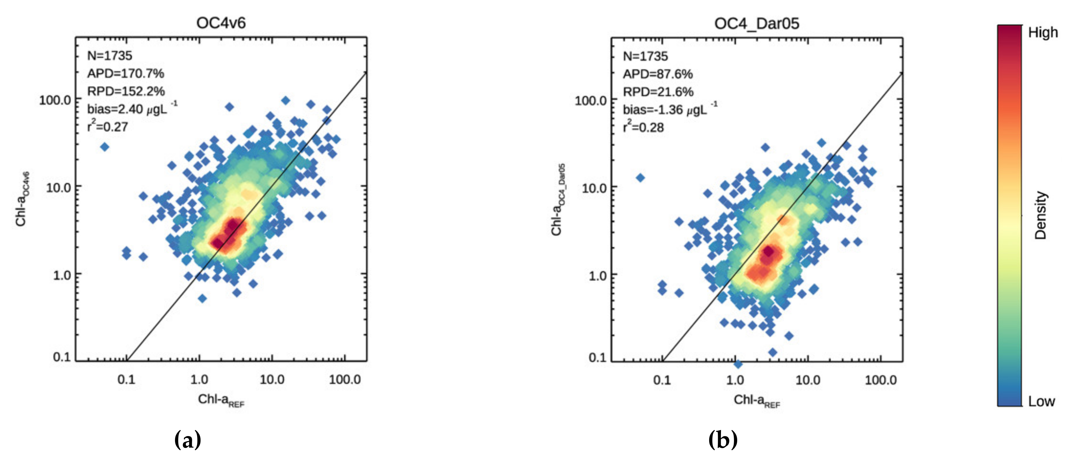
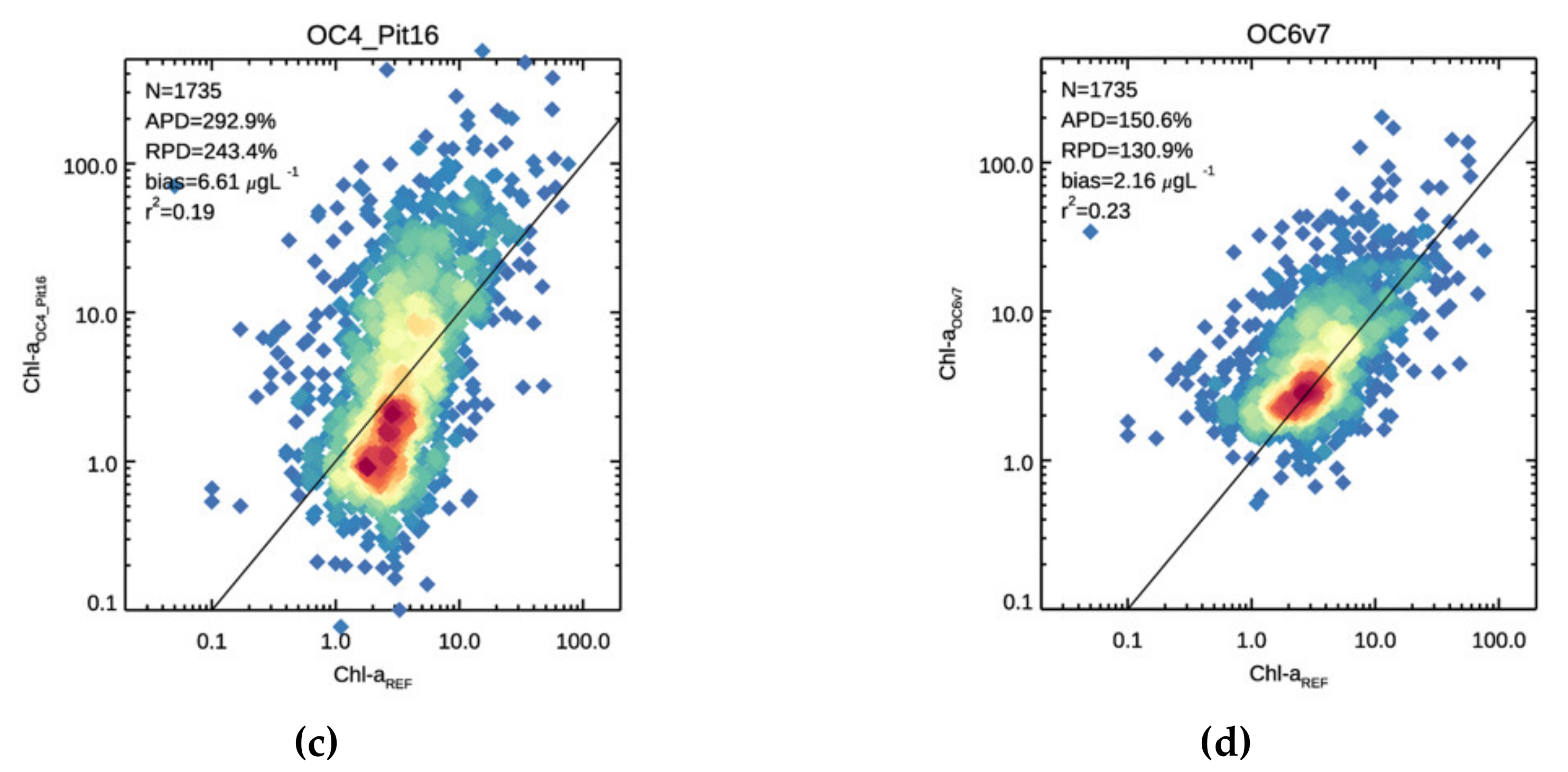
2.3. The Band-Ratio Bio-Optical Algorithms

The band-ratio algorithms considered in this work to determine chlorophyll concentration from R r s values are variants of the maximum band-ratio (MBR) algorithm presented in [63]: (1) NASA’s standard OC4v6 ( C h l - a O C 4 v 6 [47]), (2) a regional parametrization of OC4 based on field measurements ( C h l - a O C 4 _ Dar 05 [46]), (3) a recalibration of the OC4v6 achieved with a bootstrapping-like approach with in situ data previously used in CMEMS ( C h l - a O C 4 _ P i t 16 [36]), and (4) the latest version of NASA’s global algorithm OC6v7 ( C h l - a O C 6 v 7 [11]).
The algorithm equation to determine the recalibrated C h l - a O C 4 _ P i t 16 value from the OC4v6 standard results is:
l o g 10 C h l - a O C 4 _ P i t 16 = l o g 10 C h l - a O C 4 v 6 n m
with m = 0.5884 and n = 0.3751.

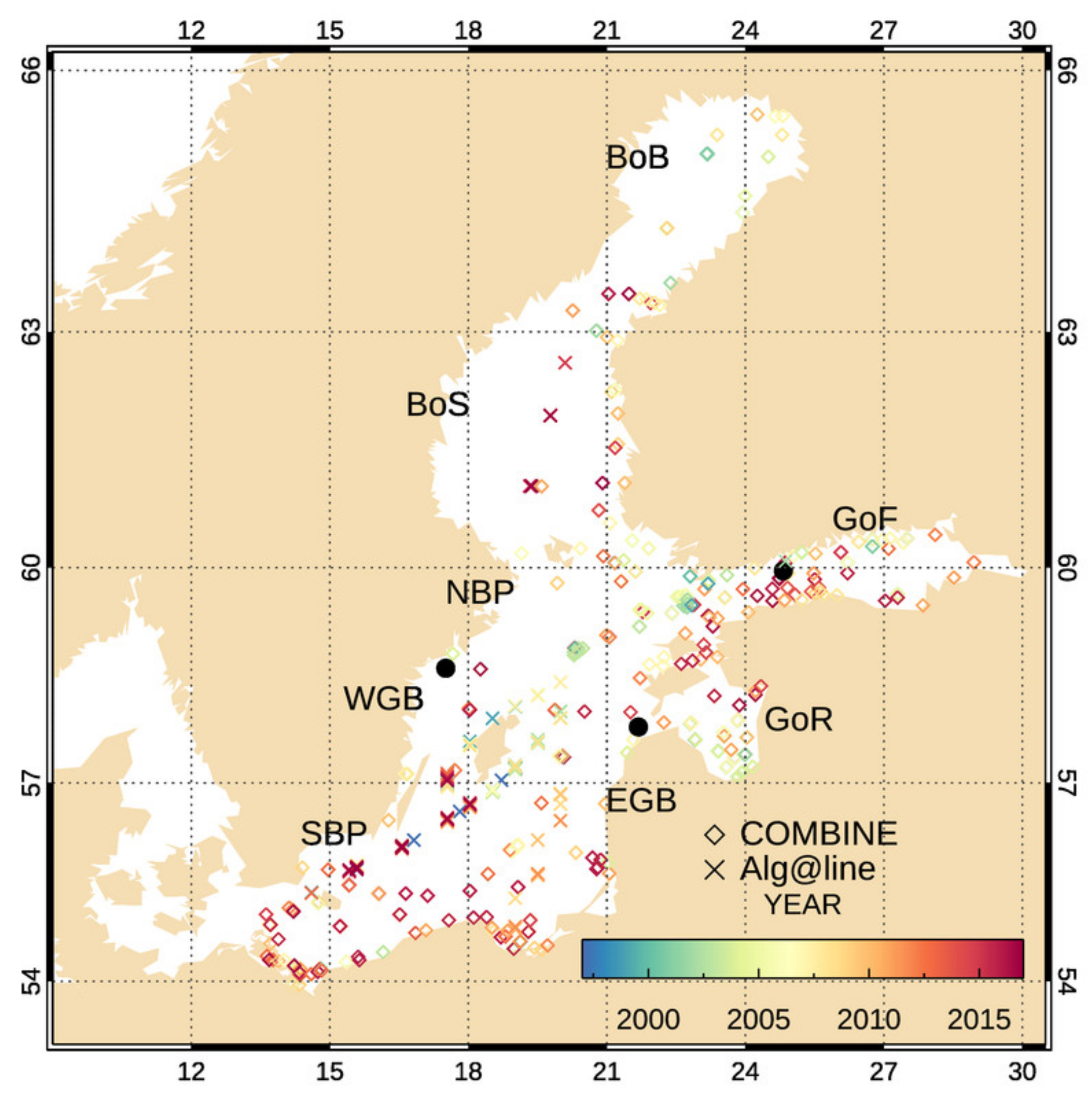
2.4. In Situ Data for Validation

2.4.1. In Situ Automated Radiometry

Reference data for the assessment of space-borne R r s spectral values were derived from field measurements acquired by the Aerosol Robotic Network-Ocean Color (AERONET-OC) at three sites in the Baltic Sea [64,65,66] (Figure 1). Data acquired between 2005 and 2019 from the Gustav Dalen Tower (58.594°N, 17.467°E), the Helsinki Lighthouse (59.949°N, 24.925°E), and the Irbe Lighthouse (57.751°N, 21.723°E) were used for independent validation. Specifically, AERONET-OC Level-2 measurements of normalized water-leaving radiance, L w N , corrected for bi-directional effects and quality-controlled as part of the operational data processing [64,65,66], were divided by the extra-solar irradiance spectrum to calculate the in situ R r s [67]. These data were then band-shifted to the CCI spectral wavelengths by means of inverse and direct application of the QAA algorithm [54,55,56]. The QAA was modified to avoid retrievals of negative phytoplankton absorption at any band that could otherwise lead to malfunctioning of the band-shift procedure.
As the AERONET-OC radiometric systems automatically operate multiple times a day, in situ and satellite potential R r s match-up spectra were chosen as the median of records collected within two hours of local noon [32]. For the satellite data, median values were extracted from a 3 × 3 box centered on the AERONET-OC sites only when at least 6 valid pixels were available, and the coefficient of variation was smaller than 20%. This led to a match-up dataset of 674 space-borne R r s spectra with both multi-sensor CCI data and corresponding in situ measurements from 2005 to 2019.

2.4.2. In Situ Data for the Assessment of the C h l - a Retrieval

Two independent in situ datasets acquired to monitor the Baltic Sea water quality (Figure 1) are utilized in the present work as a reference to assess the performance of the MLPs, their ensemble scheme, and the band-ratio regional algorithms for C h l - a retrieval.
The first set has been collected by the Finnish Environment Institute (SYKE) relying on the Alg@line acquisition system installed on ferries operating in the Helsinki–Travemünde, Helsinki–Stockholm, and Kemi–Travemünde transects [68,69]. Water samples were acquired with a flow-through setup (nominal inlet depth at 5 m), and then filtered with glass fiber filters (Whatman GF F). Chlorophyll-a was then extracted with ethanol to determine C h l - a fluorometric values [69]. The Alg@line data acquired from 1997 to 2017 were selected for this study.
The second set of records is the COMBINE database hosted by the International Council for the Exploration of the Sea (ICES), that includes C h l - a measurements collected by several institutions within the HELCOM environmental monitoring activities. C h l - a measurements were performed with techniques spanning from fluorimetry to spectrophotometry and HPLC, from the 1970s to date. All data and the different analytical protocols are subject to a well-established quality assurance policy regulated under the HELCOM COMBINE marine monitoring program [6,7]. Data acquired in the Skagerrak and Kattegat regions were not included in this analysis as the physical and optical water properties of these basins are deemed different from the actual Baltic Sea [20,26].
Space-borne C h l - a estimates for comparison with the reference field data were derived from the CCI dataset as the median of the 3 × 3 pixels box centered to the location of the in situ data point. Additional match-up criteria are: (1) a minimum of six valid pixels for the space-borne data, and (2) measurement execution for the field data between 9:00 and 15:00 (local time, i.e., 10–16 UTC) to account for the various acquisition times of the multi-sensor satellite dataset. The application of these co-location criteria resulted in 1735 records (658 and 1077 for Alg@line and COMBINE, respectively) well-distributed across the Baltic Sea (Figure 1). Due to differences in sampling strategies and techniques used for the pigment quantification, the COMBINE measurements in coastal locations cover a wider dynamic range (average C h l - a value of 5.7   μ gL 1 , 5th and 95th percentiles of 0.8 and 18.1, Table 1) than the data acquired along the Alg@line transects (average C h l - a value of 3.4   μ gL 1 , 5th and 95th percentiles of 1.1 and 7.3).
The C h l - a variability in the in situ observations (Table 1) conforms with C h l - a ranges summarized for the Baltic Sea and its sub-basins in [27]. These co-located in situ C h l - a values, utilized as a reference for the assessment of the MLP and the band-ratio bio-optical algorithms surveyed in this study, are denoted as C h l - a   R E F .

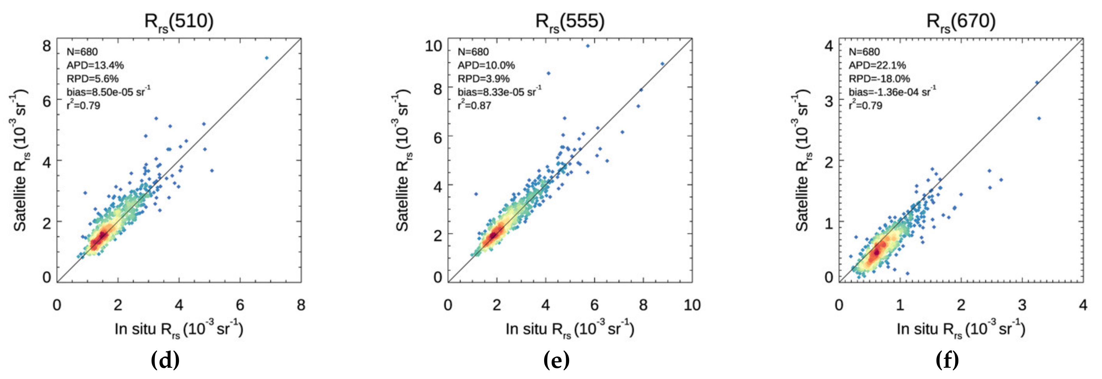
2.5. Statistical Figures

Statistical figures to evaluate the quality of results are the determination coefficient ( r 2 ), the absolute percent differences (APD), the relative percent differences (RPD), and the bias parameter between the expected x and the computed y values:
r 2 = i = 1 N x i x ¯ y i y ¯ i = 1 N x i x ¯ 2 i = 1 N y i y ¯ 2
A P D = 1 N i = 1 N y i x i x i × 100 %
R P D = 1 N i = 1 N y i x i x i × 100 %
b i a s = 1 N i = 1 N y i x i
where x ¯ and y ¯ are the mean of the expected and computed values, respectively. These parameters are applied for the assessment of C h l - a estimates, as well as R r s spectral values at each individual band. A good agreement between two datasets is achieved when r 2 is close to 1 and all the other parameters are close to 0.

2.6. Indicators of the Spring and Summer Phytoplankton Bloom Dynamics

The phytoplankton abundance and succession in the Baltic Sea are characterized by dinoflagellate- and diatom-dominated spring blooms and cyanobacterial subsurface and surface summer blooms [19,23,70]. Upon incorporating the processing improvements described in Section 2.1 and Section 2.2, the consistently reprocessed time series from 1998 to 2019 of R r s and C h l - a are used to provide an up-to-date description of Baltic Sea eutrophication state. To this aim, the indicators of the spring and summer phytoplankton bloom dynamics adopted in the CMEMS Ocean State Report [71,72] were selected.
The spring bloom dynamics are described both in terms of spatiotemporal coverage of the subsurface blooms and with the statistics for the bloom onset proposed by Groetsch et al. [73]. The occurrence of spring bloom conditions (from February to early June, i.e., over days 31–160) is thus detected on a daily basis for each pixel in the basin using a spatially variable threshold set at 5% above the median C h l - a concentration of the spring observations [73,74]. The statistics for the bloom onset, i.e., the distribution of the start as well as the peak and the end days, were calculated for each pixel in the basin and summarized using the HELCOM sub-basins [75].
For the cyanobacterial summer blooms, the spatiotemporal coverage is aggregated from estimates of daily subsurface and surface bloom, similarly to the HELCOM environmental reporting [76,77]. Summer blooms are detected on daily R r s images from June to September (i.e., days 161 to 270) by applying the thresholds on R r s at the wavelength of 555 and 670 nm defined in [78] based on visual inspection of pseudo true-color composites of MODIS imagery. These thresholds were set at R r s 555 > 4.25 × 10⁻³ sr−1 and R r s 670 > 1.22 × 10⁻³ sr−1 for the subsurface and surface blooms, respectively. This R r s -based approach to detect cyanobacterial blooms allows overcoming the difficulty of retrieving accurate C h l - a values in summer bloom conditions, as highlighted in [79,80,81]. Moreover, as cyanobacterial blooms are extremely patchy and the surface scum is unlikely to totally cover a 1 km resolution pixel [79,80,81], it is possible for both thresholds to be exceeded concurrently.
Following Hansson and Håkansson [82], cumulative maps were computed from the daily subsurface and surface images for each year and then summarized as a spatiotemporal coverage (day·km2) for both spring and summer.

3. Results

The comparisons of the space-borne R r s and the associated C h l - a estimates with respect to the in situ reference data are presented in Section 3.1 and Section 3.2, respectively. Then, the application of the time series reprocessed with the regional algorithms for environmental reporting in the Baltic Sea is demonstrated in Section 3.3.

3.1. R r s Validation

The match-up scatterplots between the co-located multi-sensor satellite and in situ R r s values are presented in Figure 3. The achieved fitness is notable in such optically complex waters for the 490–670 nm spectral range ( r 2 of 0.70–0.87, RPD of 1.3–18.0), while the 412 and 443 nm bands show higher dispersion ( r 2 of 0.05 and 0.34, RPD of 86.9% and 14.1%). For the 412–555 nm spectral range, the multi-sensor satellite R r s are overall centered on the 1:1 line, as shown by the low bias in the range 1–9 10−5 sr−1, while a larger bias (i.e., 1.36 10−4 sr−1) is observed for 670 nm. As a comparison, the global match-up summary statistics for the OC-CCI R r s are r 2 of 0.79–0.88 and bias between −7 × 10⁻⁵ and −2 × 10⁻⁴ sr−1 [12]. It should be noted that these global match-ups were based on disparate instrumentation and quality standards [12,83] featuring lower accuracy in comparison to the AERONET-OC data used as a reference in this study [84].
The satisfactory performance in the 490–670 nm spectral range and the lower accuracy reported for the blue spectral bands confirm the findings with other radiometric validation exercises carried out in the Baltic Sea [24,32,33,34,42,64,65]. Specifically, the observed bias values for R r s 555 and R r s 670 (8.33 × 10⁻⁵ and 1.36 × 10⁻⁴ sr−1, respectively) were an order of magnitude lower than the thresholds defined in [78] (i.e., 4.25 × 10⁻³ and 1.22 × 10⁻³ sr−1 for the 555 and 670 nm bands, respectively). The OC-CCI R r s were hence deemed adequate for the detection of summer subsurface and surface blooms, which will be presented in Section 3.3.2.

3.2. Chl-a Match-Ups with Alg@line Transects and COMBINE Dataset

Figure 4 and Figure 5 present the scatterplots of the satellite-derived and in situ C h l - a observations over the Baltic Sea for the regional MLP and the band-ratio algorithms described in Section 2.2 and Section 2.3. Reference values for this comparison are co-located C h l - a R E F measurements from the Alg@line transects and the data extracted from the COMBINE database. The validation statistics associated with the match-up analyses are shown in Table 2.
All proposed MLP regional algorithms present a high density of points close to the 1:1 line for the 1.0–3.0 μ gL 1   C h l - a   R E F range, but they cannot accurately retrieve C h l - a   R E F values in the 0.1–1.0 μ gL 1 range (Figure 4). Furthermore, C h l - a M L P _ 6 b and C h l - a M L P _ 4 b show some spurious retrievals of values in the 0.1–0.5 μ gL 1 range, and C h l - a M L P _ 4 b shows a tendency to saturate at 2 μ gL 1 . C h l - a M L P _ 6 b and C h l - a M L P _ 5 b are characterized by the highest dispersion (RPD of 48% and 51% and correlation coefficient of 0.137 and 0.109). C h l - a M L P _ 4 b and C h l - a M L P _ 3 b provide better results: an APD of 90% and correlation coefficient of 0.190 are reported for C h l - a M L P _ 4 b , while a bias of 0.15 μ gL 1 and correlation coefficient of 0.204 characterize C h l - a M L P _ 3 b .
The differences in the validation metrics of the four MLP candidates (Table 2) depend on the combined effect of the heterogeneous uncertainties of the satellite R r s input spectra with the applicability range of each MLP. Recalling that the reference data to evaluate C h l - a retrievals from multi-sensor R r s spectra are the Alg@line and COMBINE measurements, it is reported for comparison that the ideal performance of C h l - a M L P _ 6 b assessed with in situ measurements of C h l - a and R r s from the BiOMaP dataset attest RPD and APD values of ~9% and ~34% respectively, and a bias of −0.36 μgL−1 [45,57]. The use of R r s 412 and R r s 443 as part of the input bands for C h l - a M L P _ 6 b and C h l - a M L P _ 5 b is likely the major cause of performance degradation (note that the 412 and 443 nm bands show higher dispersion in the match-up analyses, with r 2 = 0.05 and r 2 = 0.34, respectively—see also Figure 3.
When analyzing results from the two in situ datasets separately, higher uncertainty is estimated in the match-ups with the COMBINE measurements in comparison to the water samples collected along the Alg@line transects (Table 2). For the MLP candidates, APD ranged ~42–50% for the Alg@line match-ups, while for the COMBINE dataset, it ranged 115–158%. The correlation coefficients were lower for the Alg@line (~0.05–0.12) than the COMBINE match-ups (0.095–0.193). The apparent incongruence of the opposite behavior of APD, RPD, and r 2 can be explained by different sampling strategies and the smaller dynamic range of the Alg@line observations reported in Table 1.
Among the MBRs, the match-up analyses for NASA’s standard OC4v6 ( C h l - a O C 4 v 6 [47]) and OC6v7 ( C h l - a O C 6 v 7 [11]) show a high density of points close to the 1:1 line for the 1.0–3.0 μ gL 1   C h l - a   R E F range, and a tendency to largely overestimate C h l - a   R E F for values higher than 3.0 μ gL 1 , leading to a RPD of 152% and r 2 of 0.27 for the former, and a RPD of 130% with a r 2 of 0.23 for the latter (for details, see Figure 5 and Table 2). The regional parametrization of OC4 ( C h l - a O C 4 _ Dar 05 [46]) underestimated C h l - a   R E F in the 1.0–3.0 μ gL 1 range, showing a RPD of 21.6%, a bias of –1.36 μ gL 1 , and an r 2 of 0.28. The regionally recalibrated OC4v6 previously used in CMEMS ( C h l - a O C 4 _ P i t 16 [36]) showed the highest bias (6.61   μ gL 1 ) as well as RPD and APD (243% and 292%, respectively). Similar to the MLP candidates, the match-up statistics for the MBRs also show higher APD but better correlation for the COMBINE dataset (APD = 110–437%, r 2 = 0.19–0.27), in comparison to the Alg@line transects (APD = 42–55%, r 2 = 0.08–0.13, Table 2).
An additional element to consider is that the C h l - a O C 4 _ P i t 16 statistical figures shown in Table 2 are not directly comparable with those reported in [36] due to the differences in the processing version (i.e., OC-CCI v3.1) of input R r s values, as well as heterogeneities in the match-up database. In fact, that former study [36] did not include measurements from the Alg@line transects, although it included samples from the COMBINE database acquired in the Skagerrak and Kattegat regions with physical and optical water properties that differ from those typical of the Baltic Sea (i.e., they are more similar to oceanic conditions and hence more amenable to C h l - a retrieval with OC4-like algorithms [26,36]).
The match-up analysis for two ensemble configurations ( C h l - a E N S 3 and C h l - a E N S 4 ) shows a high density of points close to the 1:1 line for the 1.0–10.0 μ gL 1   C h l - a   R E F range, and a better retrieval of C h l - a   R E F values in the 0.1–1.0 μ gL 1 range, than the MLP candidates (Figure 6). The correlation coefficients were 0.238 and 0.229, the RPD were 40.9% and 42.9%, and the bias values were −0.78 and –0.87 μgL−1 (Table 2). When considering the two in situ data sources separately, for both ensemble configurations, RPD was −24.1% and −27.4% for the Alg@line match-ups and 80.6% and 85.8% for the COMBINE dataset.
Based on the validation statistics associated with the analysis, the three-element ensemble ( C h l - a E N S 3 ) was the chosen algorithm for further analyses, as it was characterized by the lowest RPD and APD compared to the individual MLP candidates, the MBR algorithms, and C h l - a E N S 4 both for the whole match-up dataset and for the match-ups computed separately for the Alg@line transects and the COMBINE dataset (Figure 6, Table 2). The selection of the three-element ensemble relies on the full independence of the in situ Chl-a values utilized as a reference, i.e., the Alg@line and COMBINE measurement sets, with respect to the data used for the development of the MLPs as well as the weighting process underpinning the ensemble scheme. In fact, if only BiOMaP in situ data were considered for the algorithm selection, C h l - a M L P _ 6 b , i.e., the MLP with all 6 bands, would be the most performing configuration (as reported in previous investigations, e.g., [57]). However, as this study confirms, the uncertainty affecting R r s in the blue and red spectral region tends to be significantly larger for the space-borne than for the in situ data (see details in Section 3).
As shown in Figure 4, restricting the MLP input bands to a subset of the space-borne R r s spectral range (i.e., the central spectral region of the visible domain in C h l - a M L P _ 4 b and C h l - a M L P _ 3 b ) can lead to better C h l - a estimates in the Baltic Sea. The ensemble scheme has been specifically designed to account for the need for a dynamical determination of the input bands’ relevance and for spatial and temporal uncertainty of space-borne R r s values. The proposed solution automatically gives more credit, on a pixel-by-pixel basis, to the space-borne R r s spectrum (full or at a reduced number of wavelengths) more compatible with the BiOMaP in situ training data (i.e., low novelty index).

3.3. Application to Environmental Reporting

In this section, the consistently reprocessed time series of R r s and C h l - a taking-up the processing improvements presented earlier is used for environmental reporting. The same indicators of the spring and summer phytoplankton bloom dynamics adopted in the CMEMS Ocean State Report [71,72] were calculated from 1998 to 2019, thus providing an up-to-date description of the Baltic Sea eutrophication state based on previous versions of the multi-sensor time series.

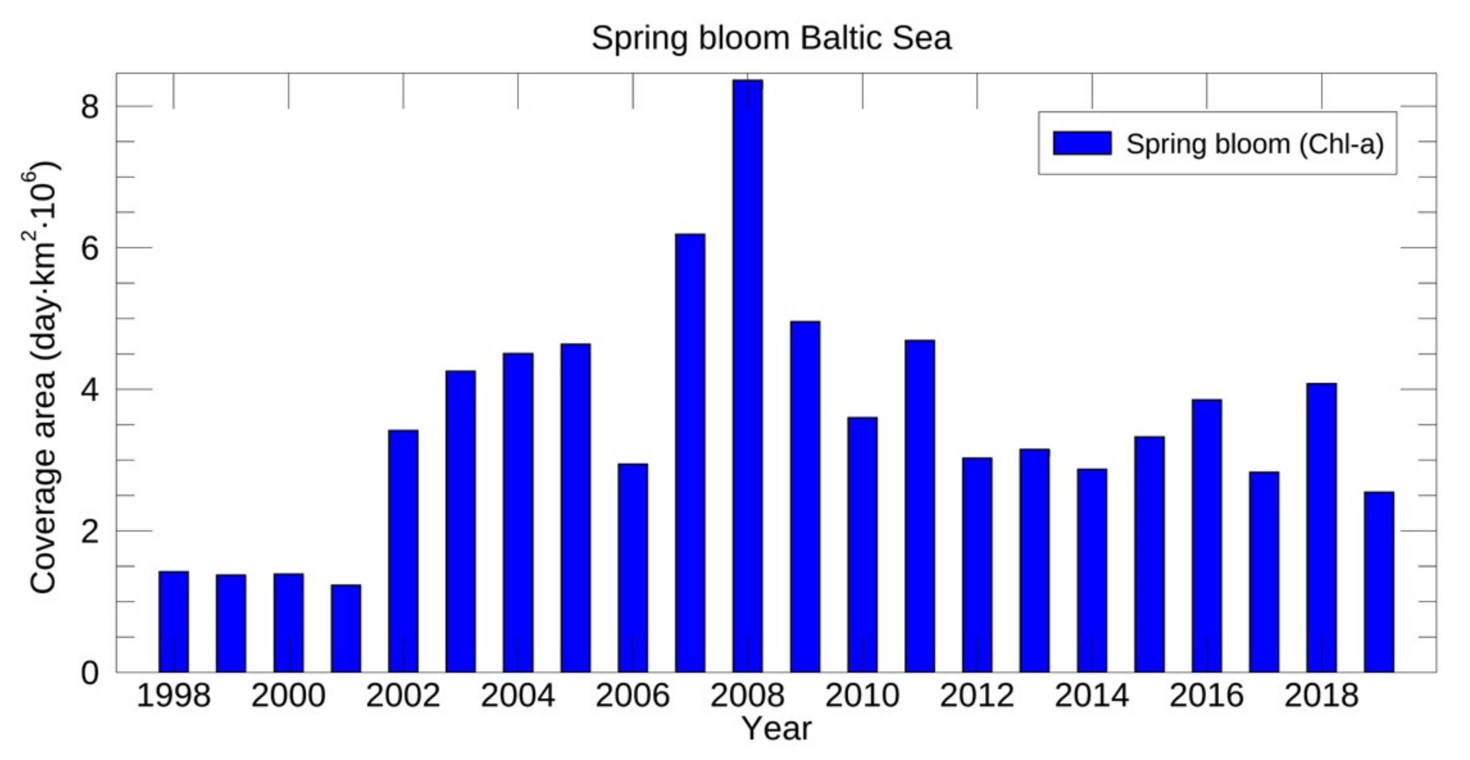
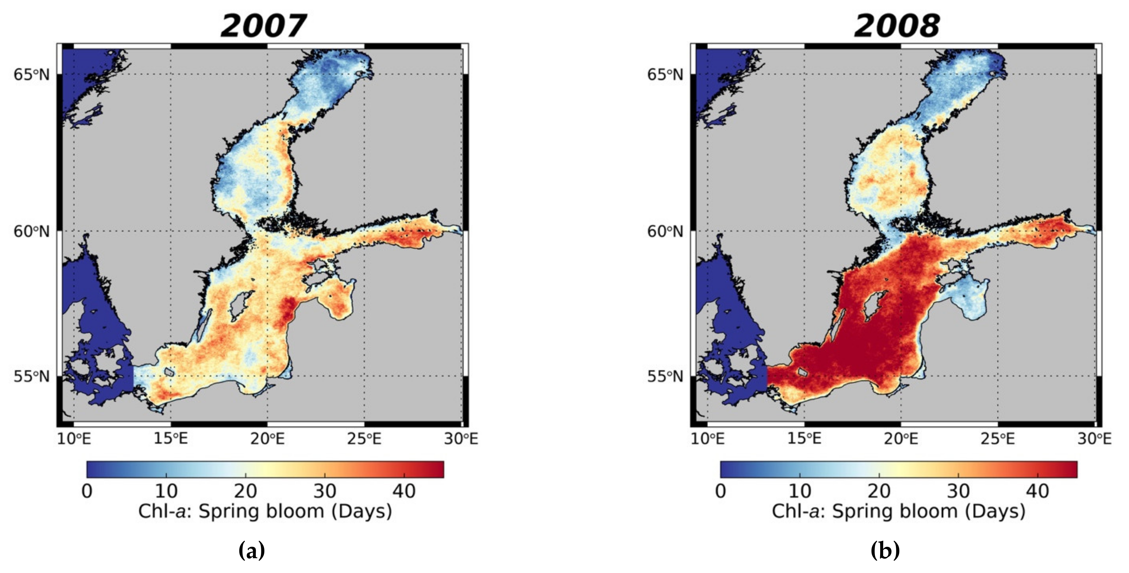
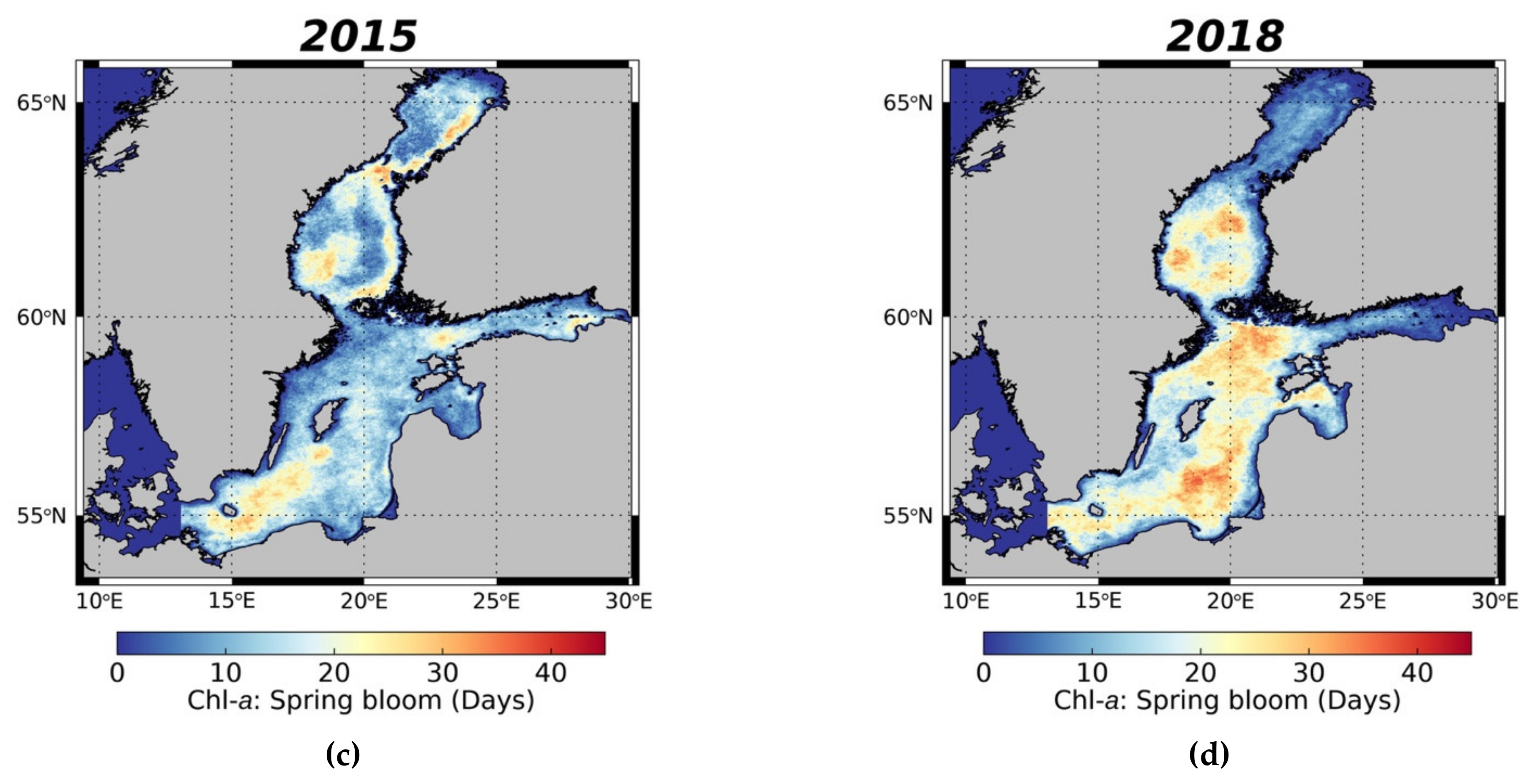
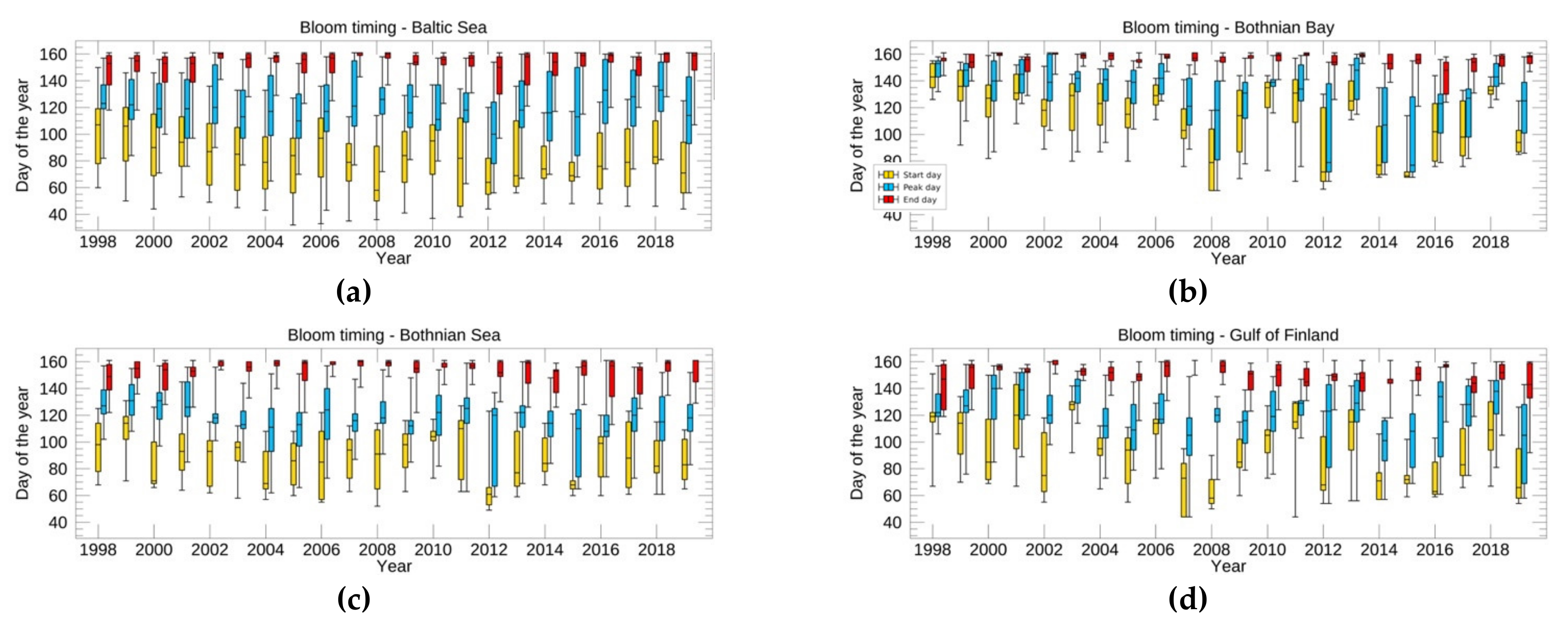
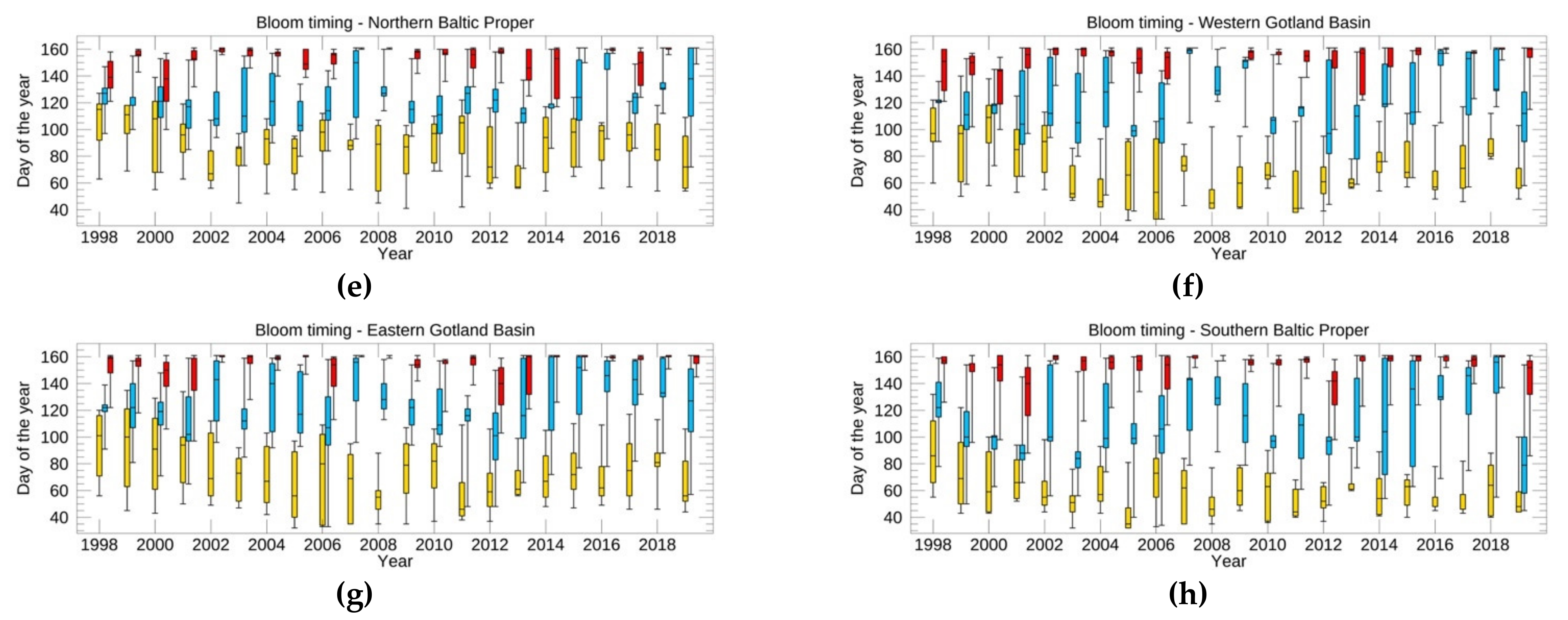
3.3.1. Spring Bloom Dynamics

This section presents the spring bloom dynamics in terms of spatiotemporal coverage (Figure 7 and Figure 8, and Figure S1) and timing (Figure 9) obtained from analyzing the C h l - a E N S 3   time series from February to early June. The method for spring bloom detection is based on a spatially explicit relative threshold derived from the C h l - a time series itself [9,73,74]. Hence, by design, the C h l - a retrieval uncertainities discussed above do not propagate to the spring bloom indicators presented in this section.
As shown in Figure 7, the bloom spatiotemporal coverage was characterized by values lower than 1.5 × 10⁶ day km2 for the years 1998–2001, then there was a general tendency to increase from 2002 to the high bloom coverage of years 2007 and 2008 (6.2 and 8.4 × 10⁶ day km2, respectively), followed by fluctuations in the range 2.5–4.9 × 10⁶ day km2. The overall behavior in spatiotemporal coverage is similar to the one reported for 1998–2017 using the same method in [71,72], but the intensities differ from the previous estimates, reflecting the C h l - a time series changes due to the improvements in the processing chain described above. The lower values observed for the spring bloom coverage in 1998–2000 compared with the coverage from 2002 onwards are consistent with the findings in [68] for GoF and NBP bloom intensity based on Alg@line C h l - a measurements. These lower estimates may also depend on the use of only SeaWiFS in 1998–2001, while two or three satellite sensors were available for the multi-sensor products merging from 2002 onwards, as a higher number of sensors could imply that a larger fraction of the basin with bloom events is captured.
As observed in previous satellite-based studies (e.g., [21,85,86]), the bloom spatiotemporal coverage varies across the sub-basins in the various years. Figure 8 presents as examples the bloom coverage for 2007, 2008, 2015, and 2018, with 2008 and 2018 showing the typical spring bloom spatial distribution and its time persistence. In 2008, the year with the highest bloom coverage within the time series, the spring bloom lasted more than 40 days across the central and southern Baltic Sea (i.e., NBP, EGB, WGB, and SBP), 20–30 days in GoF and BoS, and less than 20 days in Bob and GoR (Figure 8). In 2007, the spring bloom lasted 20–30 days in most of the basin, reaching 35 days in areas of GoF and EGB, and less than 20 days in BoB and parts of BoS. In 2018, the spring bloom lasted 15–30 days across the central and southern Baltic Sea, 20–30 days in BoS, and less than 10 days across GoF and BoB, while in 2015, the spring bloom lasted less than 15–20 days across the basin, except for some areas in SBP, BoS, and BoB, where it lasted ~20–30 days. Further variability of the spring bloom spatial distribution can be observed in the maps presented in Supplementary Figure S1.
Figure 9 provides an overview of the spring bloom timing in terms of start, peak, and end days for the Baltic Sea as a whole, and for the main sub-basins. The spatial distribution of the bloom onset within the basin for each year can be inferred by the variability in the occurrence in the start, peak, and end days, quantified by the length of the interquartile ranges (IQR) of the three dates.
Across the whole Baltic Sea (Figure 9a), the starting bloom date occurs most often from 20 February to 20 April (IQR between days 50 and 110), with the earliest onset in 2008 and 2011 (25th percentile by day 50). The IQR of the starting bloom date was ~30 days, and in 2015 the blooms occurred simultaneously, as shown by the IQR of 15 days, respectively. The peak day of spring bloom varied with no clear trend between mid-March and late-May (IQR between days 75 and 155), showing an IQR of ~30–45 days, with the blooms of 1998, 2008, and 2011 occurring simultaneously (IQR < 25 days). The end day fluctuated across the two decades, with the 75th and 95th percentiles often observed at day 160 as an effect of the definition of spring days for this analysis.
After dividing at the sub-basin level, the starting bloom date shows clear latitudinal variations, occurring most often in February–March (days 40–90) in the central and southern Baltic Sea, while the blooms start later in the two northern basins: March–April (days 60–120) in BoS and March–May (days 60–150) in BoB, due to the longer duration of the ice cover. Overall, there was a general trend for all sub-basins of earlier phytoplankton blooms by 1–3 weeks across the two decades in terms of start and peak dates that was clearly visible for the distribution of the bloom onset calculated for the whole basin. This confirms the lengthening of the bloom period observed in [73] for GoF, NBP, and SBP based on Alg@line Chl-a measurements, and the early blooming reported in [19] based on an intensive sampling of phytoplankton and hydro-chemical parameters at selected sites in GoF and NBP. The earlier appearance of spring blooms in the last decades has been linked to climate warming [19,68], although spatially explicit studies across the whole Baltic Sea are still missing.
Figure 9 shows that 2008 was an anomalous year also in terms of the bloom timing, particularly for BoB, where the bloom started on day 60–90, almost a month earlier than usual. Furthermore, the peak day IQR for the whole Baltic Sea for 2008 was small as the bloom peaked almost simultaneously within most sub-basins, as shown by the individual IQRs. The division at the sub-basin level also highlights the early onset and peak of the 2015 bloom in the BoB: the starting bloom date was around day 70 and it was followed by an early peak (median peak day 77), consistent with the sea-ice coverage anomaly that occurred in the winter of 2014/2015, when BoB, for the first time, remained partially ice-free [87].

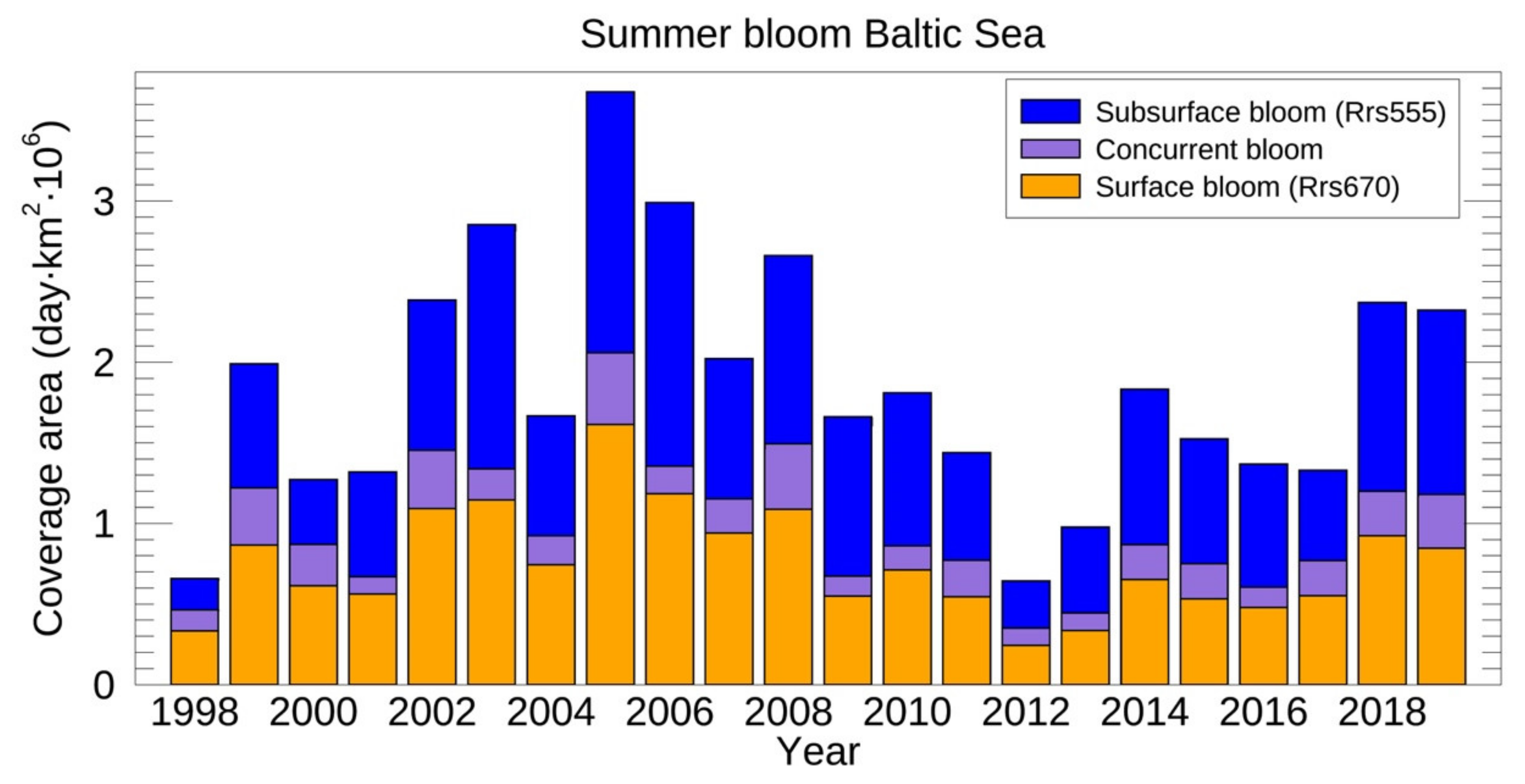
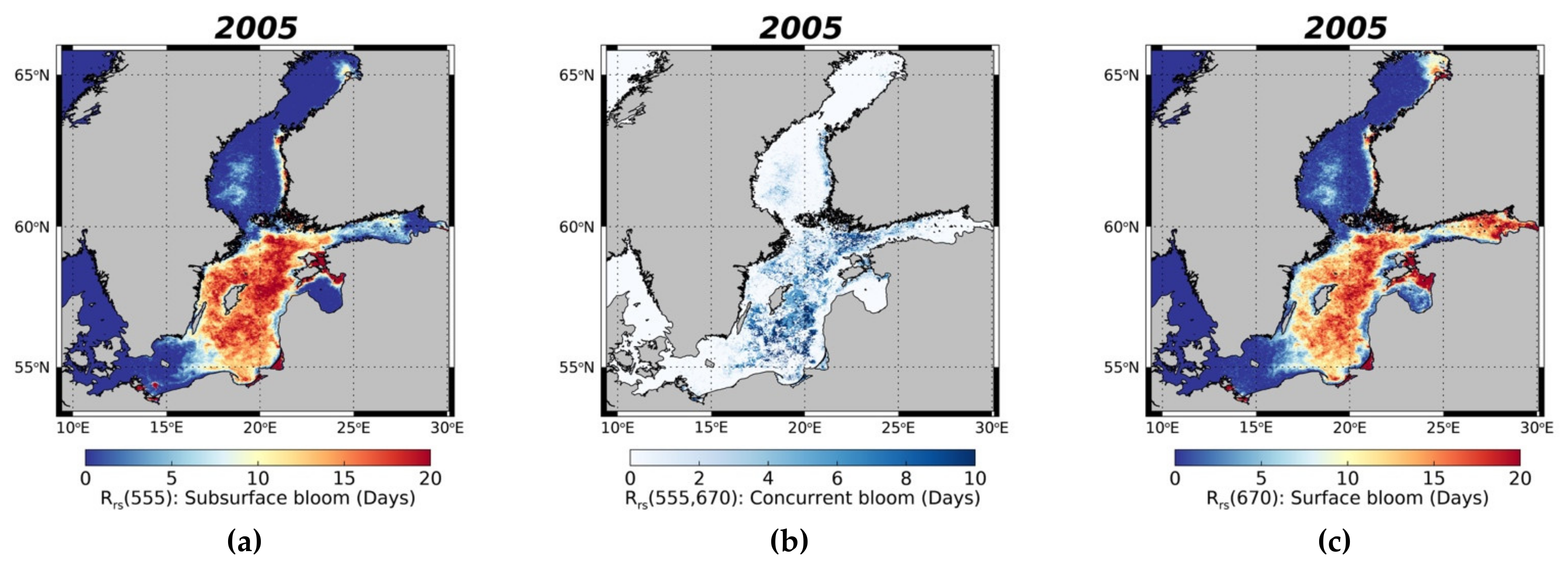
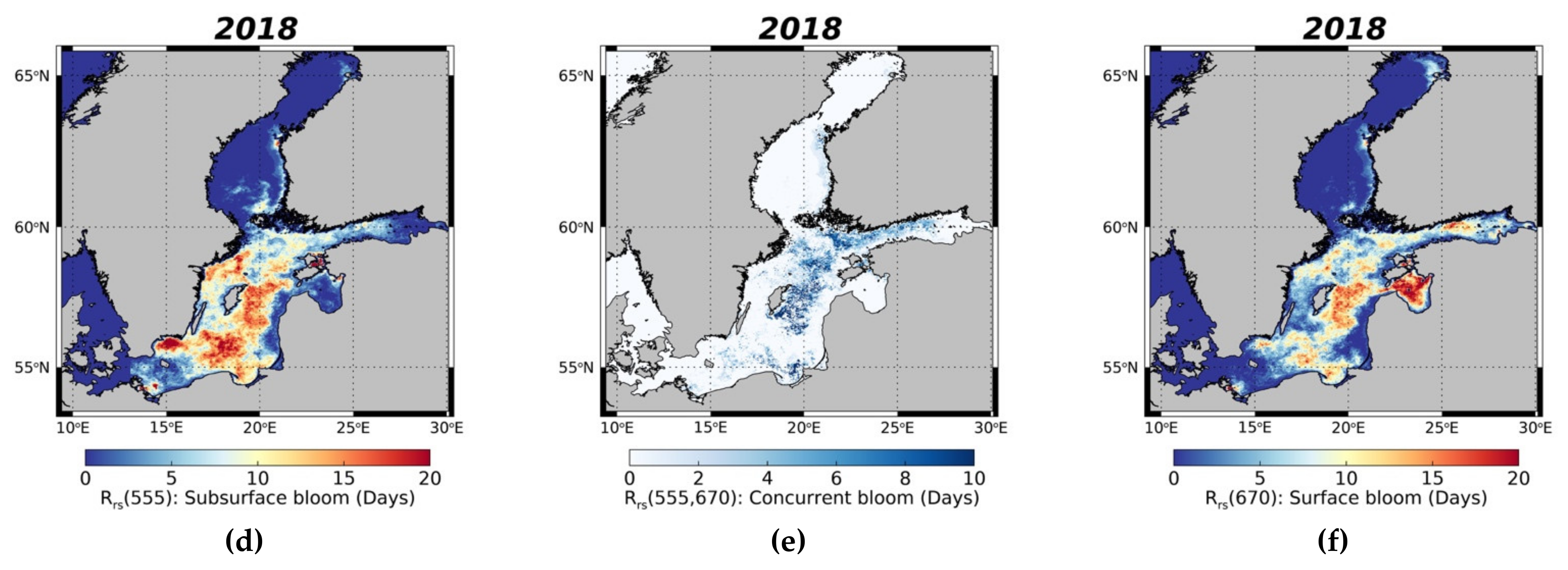
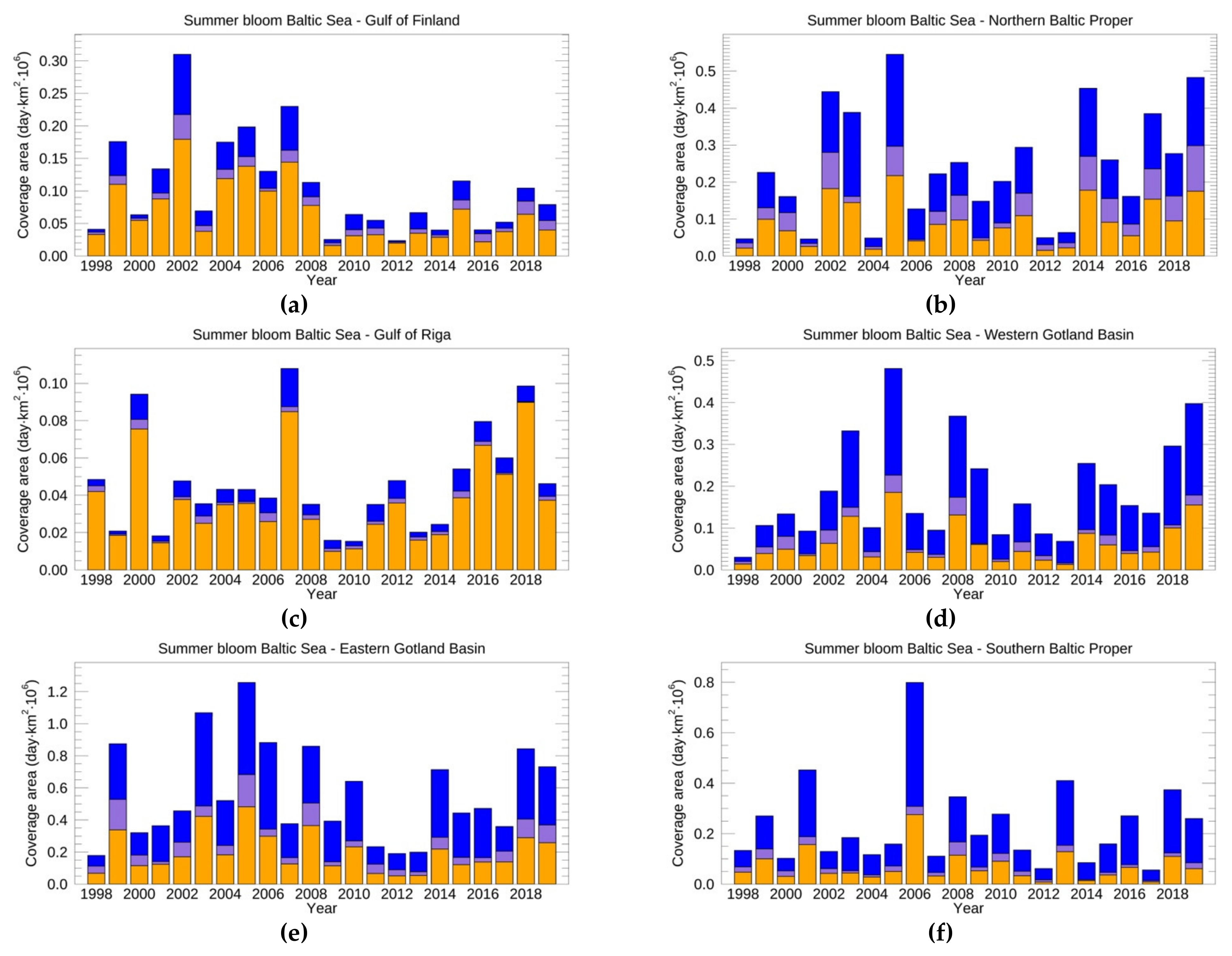
3.3.2. Surface and Subsurface Summer Blooms

In the Baltic Sea, the phytoplankton blooms occurring during summer are dominated by nitrogen-fixing cyanobacteria. These blooms can have subsurface and/or surface accumulations, depending on the age of the bloom. This section presents the dynamics of cyanobacterial summer blooms with the spatiotemporal coverage estimated from the reprocessed time series of multi-sensor R r s , thus avoiding the possible low-accuracy retrievals for Chl-a in cyanobacterial bloom conditions.
The time series of total coverage of surface and subsurface blooms in summer is presented in Figure 10 for the whole basin. Overall, the summer bloom coverage increased from 1998 to 2005, decreased from 2005 to 2012, and then increased from 2012 to date, showing oscillations without a consistent decadal trend, as observed from 1979 to date [23,86,88]. The largest summer coverage blooms of the 1998–2019 time series were observed for 2005 and 2006, with a coverage of ~3.6 and 3.0 × 10⁶ day km2, respectively. The summer bloom coverage was dominated by surface blooms in 1998–2007 and by subsurface blooms in the latter part of the time series. The area with concurrent surface and subsurface cyanobacterial bloom, i.e., where both thresholds were exceeded, was on average 12.7% of the total coverage (ranging ~1.1 and 4.4 × 10⁵ day km2), with the maximum concurrent extent recorded in 2005.
Summer blooms appear in the different sub-regions with different magnitude (Figure 11 and Figure S1). In 2005, the year with the largest summer bloom coverage, the subsurface bloom lasted 10–20 days across the central Baltic Sea (NBP, EGB, and WGB), and the surface bloom lasted 10–20 days across the central Baltic Sea and GoF (Figure 11). The subsurface and surface blooms occurred concurrently in most of the central Baltic Sea for 5–10 days. In 2018, the subsurface bloom lasted 10–15 day across the central and Southern Baltic Sea (mostly WGB, EGB, and SBP; NBP 5–15 days), and the surface bloom lasted 10–20 days across the central and Southern Baltic Sea, as well as GoR and patches in the central GoF. The subsurface and surface blooms occurred concurrently for parts of EGB, NBP, and GoF for 5–8 days.
At the sub-basin scale (Figure 12 and Figure S1), several summer bloom events (e.g., in 2002, 2003, and 2005) occurred in the central regions (WGB, EGB, NBP), as also reported in [21,85]. In these central basins, the surface and subsurface summer blooms were of similar extents and the areas where both thresholds were exceeded ranged on average 10–20% of the total coverage. The extensive bloom that occurred in 2005, as shown by our analysis, is reinforced by the HELCOM report, that shows similar nutrient concentrations in 2004 and 2005, with double phosphate levels in the surface [89]. Nevertheless, the weather conditions (cold temperature and wind) of 2004 were not suitable for the onset of a cyanobacterial bloom. On the contrary, the warmer temperature, light conditions of summer 2005, in addition to the excess dissolved inorganic phosphorus, resulted in an intense bloom, covering the central area as WGB, EGB, and NBP [77].
The summer bloom events in GoF, GoR, and SBP differed from those observed in the central regions in terms of timing and of the surface and subsurface extents. The GoF summer blooms were dominated by the surface expression and occurred mostly in the first decade, with a peak in 2002. In GoR, summer blooms were characterized by a larger surface component, and the main events occurred in 2000, 2007, 2016, and 2018 when limited summer bloom extents were observed in the central regions. The blooms in SBP were characterized by a larger subsurface component and peaked in 2001, 2006, and 2013 when the bloom extensions were low for NBP and WGB.

4. Discussion and Conclusions

This study presented recent improvements for the 1997–2019 C h l - a time series determined for the Baltic Sea from space-borne multi-sensor data. The accuracy of OC-CCI R r s for the Baltic Sea was assessed with AERONET-OC data acquired from 2005 to 2019 at three sites located in different sub-basins [64,65,66]. In agreement with other studies [64,65], results from the analysis of R r s match-up data showed that the external bands (412 and 670 nm) are affected by larger uncertainties: R r s 412 was characterized by a high dispersion, while R r s 670 had the largest bias. The OC-CCI R r s were deemed adequate for the detection of summer surface blooms as the observed bias values for R r s 555 and R r s 670 were an order of magnitude lower than the adopted thresholds.
The proposed ensemble scheme represents a new paradigm with respect to the a priori classification of the input R r s and associated Chl - a retrieval algorithms [12,15,41,90,91]. Namely, the study considered that: (1) the R r s match-up analysis has shown that the atmospheric correction process can induce larger uncertainties in the blue spectral region, (2) when accurate, input bands in the blue spectral region can improve the MLP performance, but (3) degradation of results and reduction of the MLP applicability range occur when uncertainties increase. The ensemble solution was thus devised to exploit the information embedded in the blue spectral bands only when the overall space-born input R r s spectrum is compatible withthe in situ data used for MLP training, taking the agreement with the field measurements as an indication of well-performing atmospheric correction on a pixel-by-pixel basis. For low values of the novelty index, the MLPs based on the extended spectral range will contribute with high weights to define the ensemble result.
The ensemble scheme hence permits to account for the temporal and spatial variation of uncertainties induced by the atmospheric correction process. The result is a dynamical relevance determination of Chl-a values derived from R r s at different sets of bands. The effectiveness of the proposed scheme is heuristically endorsed by the higher quality of the retrieved Chl-a values, as assessed with the reference Alg@line and COMBINE measurements not considered for the MLP training. Results based on these two independent reference datasets have shown that the proposed ensemble scheme consistently outperformed the Chl-a retrievals by alternative schemes (i.e., standard and regional band-ratio algorithms, as well as individual MLPs) [11,36,46,47]. The matchup statistics achieved in this study with the ensemble scheme (correlation coefficient of 0.238, RPD of 40.9%, and bias value of −0.78 μgL−1) may appear as unsatisfactory, but represent a considerable reduction of the gross C h l - a overestimates induced by the high CDOM in the Baltic Sea documented by studies based on SeaWiFS and MODIS band-sets [25,26,27,35,36,37]. Raising the accuracy of C h l - a retrievals in the Baltic Sea above the level attained in this work with the ensemble scheme largely depends on atmospheric correction improvements in the blue and red spectral regions. Since the reprocessed multi-sensor time series of R r s spectra are determined at the wavelengths of the SeaWiFS sensor, the C2RCC and ONNS neural nets could not be applied in this work due to differences in input spectral bands [24,40,41]. Note also that the Chl-a assessments in the present study considered the whole basin, while several previous studies addressed a sub-basin level, possibly enhancing the reported performance at those scales [25,39,40,42,46].
The optical variability over short spatial scales, as well as the patchiness in C h l - a concentrations and of cyanobacterial blooms in the basin, are the likely sources of the high dispersion reported in the match-up analyses with the 1 km resolution pixel [30,31,42,79,80,81]. The heterogeneity of statistical results is documented by the higher uncertainty estimated with the COMBINE dataset in comparison to the water samples collected along the Alg@line transects. An analogous finding was reported for OLCI imagery by Toming et al. [42], with different uncertainties between coastal waters and the Baltic Proper. A further factor contributing to the reported dispersion of the match-ups’ data points is the large co-location time window due to the lack of exact acquisition time for the multi-sensor dataset.
The 1997–2019 time series of the R r s and C h l - a are freely available at the CMEMS portal. The time series will be extended as part of the CMEMS operational processing on a six-month basis. The use of a combined MERIS and OLCI time series at a spatial resolution of 300 m would most probably lead to increased accuracy on the C h l - a retrieval, as several algorithms make use of the extended spectral band-set [24,26,41]. However, this time series would span 2002–2012 and then 2016 onwards and would not benefit from the increased spatial coverage brought by the multi-sensor merging.
The consistently reprocessed time series of C h l - a and R r s presented in this study allowed for a comprehensive description of the phytoplankton bloom evolution for spring and summer seasons. The overall magnitude and the interannual variability of the spring and summer blooms described in this work is coherent with the literature [19,21,68,73,85,86]. The analysis of the phytoplankton dynamics at sub-basin levels enabled detailing the latitudinal variations in the spring bloom phenology across the basin, and offered the first documentation at basin and sub-basin scales of the earlier onset and the lengthening of the spring bloom over the last two decades. These spatially explicit findings confirm and extend the results based on in situ observations [19,68,73].
The quantification of the Baltic Sea surface and subsurface summer blooms was complemented for the first time by an assessment of the blooms with concurrent surface and subsurface expression. The summer blooms occurred more frequently in the central Baltic Sea, differing from Gulf of Finland, Gulf of Riga, and Southern Baltic Proper, in terms of timing as well as surface and subsurface extents. These findings are in overall accordance with previous satellite-based studies and the HELCOM results [21,76,77,85,86,89], even if due to changes in the input satellite imagery and detection method, the HELCOM remote sensing indexes computed from 2010 onwards cannot be directly compared with the 1997 to 2009 values [76,77,82].
Nowadays, satellite sensors provide data for extensive spatial and temporal monitoring of phytoplankton variability. In the context of the Good Environmental Status actions, the present study demonstrates how the eutrophication assessment in the Baltic Sea can be deeply reinforced by the use of Earth Observation data. The combined use of space-borne and in situ information (monitoring stations and field activities) has to be aimed to achieve a good status in all regions of this basin and prevent negative effects of eutrophication.

Supplementary Materials

The following are available online at https://www.mdpi.com/article/10.3390/rs13163071/s1. Figure S1: Spring and Summer Bloom spatio-temporal coverage from 1998 to 2019. First column: Spring bloom; second column: subsurface Summer bloom; third column: concurrent subsurface and surface summer bloom; fourth column: Surface summer bloom. Table S1: Parameters set for C h l - a M L P _ 6 b . Table S2: Parameters set for C h l - a M L P _ 5 b . Table S3: Parameters set for C h l - a M L P _ 4 b . Table S4: Parameters set for C h l - a M L P _ 3 b .

Author Contributions

Conceptualization, V.E.B., D.D., and M.S.; methodology, V.E.B., D.D., and M.S.; software, V.E.B., S.C., D.D., and M.S.; validation, V.E.B., M.B., A.D.C., and M.S.; formal analysis, V.E.B. and M.S.; in situ data curation, J.A., M.B., S.C., and S.K.; satellite data curation, S.C.; writing—original draft preparation, V.E.B., D.D., and M.S.; writing—review and editing, J.A., M.B., S.C., A.D.C., and T.K.; visualization, V.E.B. and M.S.; supervision, V.E.B. and D.D.; project administration, V.E.B.; funding acquisition, V.E.B. and D.D. All authors have read and agreed to the published version of the manuscript.

Funding

This work has been performed in the context of the Ocean Colour Thematic Assembly Centre of the Copernicus Marine Environment and Monitoring Service (grant number: 77-CMEMS-TAC-OC).

Institutional Review Board Statement

Not applicable.

Informed Consent Statement

Not applicable.

Data Availability Statement

The fully consistently reprocessed R r s and Chl-a time series are available for download on the CMEMS web portal (http://marine.copernicus.eu/ accessed on 25 June 2021) as products OCEANCOLOUR_BAL_CHL_L3_REP_OBSERVATIONS_009_080 and OCEANCOLOUR_BAL_OPTICS_L3_REP_OBSERVATIONS_009_097.

Acknowledgments

R r s spectra at 1 km resolution were produced by the Plymouth Marine Laboratory (PML) using the OC-CCI processor within the Ocean Colour Thematic Assembly Centre activities. The AERONET Team is acknowledged for the continuous effort in supporting the AERONET-OC sub-network. Giuseppe Zibordi from the Joint Research Center of the European Commission is acknowledged for establishing and maintaining the Irbe Lighthouse, Gustav Dalen Tower, and Helsinki Lighthouse AERONET-OC sites, and for providing access to the BIOMAP dataset. ICES and HELCOM along with all single contributors are thanked for the COMBINE in situ dataset. Scientists and technical personnel at SYKE are thanked for the acquisition of the Alg@line in situ dataset. We are grateful to Vega Forneris and Flavio Lapadula for maintaining the satellite data processing and the satellite data archive at CNR-ISMAR. We thank the three reviewers and the academic editor for their insightful and constructive comments that helped strengthening the manuscript.

Conflicts of Interest

The authors declare no conflict of interest. The funders had no role in the design of the study; in the collection, analyses, or interpretation of data; in the writing of the manuscript, or in the decision to publish the results.

References

  1. Andersen, J.H.; Axe, P.; Backer, H.; Carstensen, J.; Claussen, U.; Fleming-Lehtinen, V.; Järvinen, M.; Kaartokallio, H.; Knuuttila, S.; Korpinen, S.; et al. Getting the Measure of Eutrophication in the Baltic Sea: Towards Improved Assessment Principles and Methods. Biogeochemistry 2011, 106, 137–156. [Google Scholar] [CrossRef] [Green Version]
  2. Fleming-Lehtinen, V.; Andersen, J.H.; Carstensen, J.; Łysiak-Pastuszak, E.; Murray, C.; Pyhälä, M.; Laamanen, M. Recent developments in assessment methodology reveal that the baltic sea eutrophication problem is expanding. Ecol. Indic. 2015, 48, 380–388. [Google Scholar] [CrossRef] [Green Version]
  3. HELCOM. HELCOM Baltic Sea Action Plan; HELCOM: Helsinki, Finland, 2007. [Google Scholar]
  4. HELCOM. State of the Baltic Sea—Second HELCOM Holistic Assessment 2011–2016; HELCOM: Helsinki, Finland, 2018. [Google Scholar]
  5. Malone, T.C.; Newton, A. The globalization of cultural eutrophication in the coastal ocean: Causes and consequences. Front. Mar. Sci. 2020, 7, 670. [Google Scholar] [CrossRef]
  6. HELCOM. Manual for Marine Monitoring in the COMBINE Programme of HELCOM; HELCOM: Helsinki, Finland, 2017. [Google Scholar]
  7. HELCOM. HELCOM Guidelines for Monitoring of Chlorophyll a; HELCOM: Helsinki, Finland, 2019. [Google Scholar]
  8. Ahlman, M.; Alenius, P.; Attila, J.; Arnkil, A.; Arponen, H.; Below, A.; Blankett, P.; Bäck, A.; Cederberg, T.; Forsman, L.; et al. Seurantakäsikirja Suomen Merenhoitosuunnitelman Seurantaohjelmaan Vuosille 2020–2026 (Manual for Marine Monitoring in Finland 2020–2026).; Suomen Ympäristökeskus: Helsinki, Finland, 2020; ISBN 978-952-11-5340-2. [Google Scholar]
  9. Blondeau-Patissier, D.; Gower, J.F.R.; Dekker, A.G.; Phinn, S.R.; Brando, V.E. A review of ocean color remote sensing methods and statistical techniques for the detection, mapping and analysis of phytoplankton blooms in coastal and open oceans. Prog. Oceanogr. 2014, 123, 123–144. [Google Scholar] [CrossRef] [Green Version]
  10. Groom, S.; Sathyendranath, S.; Ban, Y.; Bernard, S.; Brewin, R.; Brotas, V.; Brockmann, C.; Chauhan, P.; Choi, J.; Chuprin, A.; et al. Satellite Ocean Colour: Current Status and Future Perspective. Front. Mar. Sci. 2019, 6, 485. [Google Scholar] [CrossRef] [Green Version]
  11. O’Reilly, J.E.; Werdell, P.J. Chlorophyll Algorithms for Ocean Color Sensors—OC4, OC5 & OC6. Remote. Sens. Environ. 2019, 229, 32–47. [Google Scholar] [CrossRef]
  12. Sathyendranath, S.; Brewin, R.; Brockmann, C.; Brotas, V.; Calton, B.; Chuprin, A.; Cipollini, P.; Couto, A.; Dingle, J.; Doerffer, R.; et al. An ocean-colour time series for use in climate studies: The experience of the ocean-colour climate change initiative (OC-CCI). Sensors 2019, 19, 4285. [Google Scholar] [CrossRef] [PubMed] [Green Version]
  13. Sathyendranath, S.; Brewin, R.J.W.; Jackson, T.; Mélin, F.; Platt, T. Ocean-colour products for climate-change studies: What are their ideal characteristics? Remote. Sens. Environ. 2017, 203, 125–138. [Google Scholar] [CrossRef] [Green Version]
  14. Szeto, M.; Werdell, P.J.; Moore, T.S.; Campbell, J.W. Are the world’s oceans optically different? J. Geophys. Res. 2011, 116, C00H04. [Google Scholar] [CrossRef] [Green Version]
  15. Volpe, G.; Colella, S.; Brando, V.E.; Forneris, V.; La Padula, F.; Di Cicco, A.; Sammartino, M.; Bracaglia, M.; Artuso, F.; Santoleri, R. Mediterranean Ocean Colour Level 3 Operational Multi-Sensor Processing. Ocean Sci. 2019, 15, 127–146. [Google Scholar] [CrossRef] [Green Version]
  16. Heiskanen, A.-S.; Bonsdorff, E.; Joas, M. Baltic Sea: A Recovering Future From Decades of Eutrophication. In Coasts and Estuaries; Elsevier: Amsterdam, The Netherlands, 2019; pp. 343–362. ISBN 978-0-12-814003-1. [Google Scholar]
  17. Kahru, M.; Horstmann, U.; Rud, O. Satellite detection of increased cyanobacteria blooms in the Baltic Sea: Natural fluctuation or ecosystem change? Ambio 1994, 23, 469–472. [Google Scholar]
  18. Leppäranta, M.; Myrberg, K. Physical Oceanography of the Baltic Sea; Springer: Berlin/Heidelberg, Germany, 2009; ISBN 978-3-540-79702-9. [Google Scholar]
  19. Hjerne, O.; Hajdu, S.; Larsson, U.; Downing, A.S.; Winder, M. Climate driven changes in timing, composition and magnitude of the Baltic Sea Phytoplankton Spring Bloom. Front. Mar. Sci. 2019, 6. [Google Scholar] [CrossRef] [Green Version]
  20. Simis, S.G.H.; Ylöstalo, P.; Kallio, K.Y.; Spilling, K.; Kutser, T. Contrasting seasonality in optical-biogeochemical properties of the Baltic Sea. PLoS ONE 2017, 12, e0173357. [Google Scholar] [CrossRef]
  21. Zhang, D.; Lavender, S.; Muller, J.-P.; Walton, D.; Zou, X.; Shi, F. MERIS observations of phytoplankton phenology in the Baltic Sea. Sci. Total. Environ. 2018, 642, 447–462. [Google Scholar] [CrossRef]
  22. Finni, T.; Kononen, K.; Olsonen, R.; Wallström, K. The history of cyanobacterial blooms in the Baltic Sea. Ambio 2001, 30, 172–178. [Google Scholar] [CrossRef]
  23. Kahru, M.; Elmgren, R.; Di Lorenzo, E.; Savchuk, O. Unexplained interannual oscillations of cyanobacterial blooms in the Baltic Sea. Sci. Rep. 2018, 8, 6365. [Google Scholar] [CrossRef] [PubMed] [Green Version]
  24. Attila, J.; Koponen, S.; Kallio, K.; Lindfors, A.; Kaitala, S.; Ylöstalo, P. MERIS Case II Water Processor Comparison on Coastal Sites of the Northern Baltic Sea. Remote. Sens. Environ. 2013, 128, 138–149. [Google Scholar] [CrossRef]
  25. Darecki, M.; Stramski, D. An Evaluation of MODIS and SeaWiFS Bio-Optical Algorithms in the Baltic Sea. Remote. Sens. Environ. 2004, 89, 326–350. [Google Scholar] [CrossRef]
  26. Ligi, M.; Kutser, T.; Kallio, K.; Attila, J.; Koponen, S.; Paavel, B.; Soomets, T.; Reinart, A. Testing the performance of empirical remote sensing algorithms in the Baltic Sea waters with modelled and in situ reflectance data. Oceanologia 2017, 59, 57–68. [Google Scholar] [CrossRef] [Green Version]
  27. Kratzer, S.; Moore, G. Inherent optical properties of the Baltic Sea in comparison to other seas and oceans. Remote. Sens. 2018, 10, 418. [Google Scholar] [CrossRef] [Green Version]
  28. Berthon, J.-F.; Zibordi, G. Optically black waters in the Northern Baltic Sea. Geophys. Res. Lett. 2010, 37. [Google Scholar] [CrossRef]
  29. Zibordi, G.; Berthon, J.-F.; Mélin, F.; D’Alimonte, D. Cross-Site Consistent in Situ Measurements for Satellite Ocean Color Applications: The BiOMaP Radiometric Dataset. Remote. Sens. Environ. 2011, 115, 2104–2115. [Google Scholar] [CrossRef]
  30. Aavaste, A.; Sipelgas, L.; Uiboupin, R.; Uudeberg, K. Impact of thermohaline conditions on vertical variability of optical properties in the Gulf of Finland (Baltic Sea): Implications for water quality remote sensing. Front. Mar. Sci. 2021, 8. [Google Scholar] [CrossRef]
  31. Scheinin, M.; Asmala, E. Ubiquitous Patchiness in Chlorophyll a Concentration in Coastal Archipelago of Baltic Sea. Front. Mar. Sci. 2020, 7, 563. [Google Scholar] [CrossRef]
  32. Mélin, F.; Zibordi, G.; Berthon, J.-F.; Bailey, S.; Franz, B.; Voss, K.; Flora, S.; Grant, M. Assessment of MERIS Reflectance Data as Processed with SeaDAS over the European Seas. Opt. Express 2011, 19, 25657–25671. [Google Scholar] [CrossRef] [PubMed] [Green Version]
  33. Qin, P.; Simis, S.G.H.; Tilstone, G.H. Radiometric Validation of Atmospheric Correction for MERIS in the Baltic Sea Based on Continuous Observations from Ships and AERONET-OC. Remote. Sens. Environ. 2017, 200, 263–280. [Google Scholar] [CrossRef] [Green Version]
  34. Zibordi, G.; Melin, F.; Berthon, J.-F. A Regional Assessment of OLCI Data Products. IEEE Geosci. Remote Sens. Lett. 2018, 15, 1490–1494. [Google Scholar] [CrossRef]
  35. D’Alimonte, D.; Kajiyama, T.; Saptawijaya, A. Ocean color remote sensing of atypical marine optical cases. IEEE Trans. Geosci. Remote Sens. 2016, 54, 6574–6586. [Google Scholar] [CrossRef]
  36. Pitarch, J.; Volpe, G.; Colella, S.; Krasemann, H.; Santoleri, R. Remote Sensing of Chlorophyll in the Baltic Sea at Basin Scale from 1997 to 2012 Using Merged Multi-Sensor Data. Ocean Sci. 2016, 12, 379–389. [Google Scholar] [CrossRef] [Green Version]
  37. Odermatt, D.; Gitelson, A.; Brando, V.E.; Schaepman, M. Review of constituent retrieval in optically deep and complex waters from satellite imagery. Remote Sens. Environ. 2012, 118, 116–126. [Google Scholar] [CrossRef] [Green Version]
  38. D’Alimonte, D.; Zibordi, G.; Berthon, J.-F.; Canuti, E.; Kajiyama, T. Performance and Applicability of Bio-Optical Algorithms in Different European Seas. Remote Sens. Environ. 2012, 124, 402–412. [Google Scholar] [CrossRef]
  39. Kratzer, S.; Vinterhav, C. Improvement of MERIS Level 2 Products in Baltic Sea Coastal Areas by Applying the Improved Contrast between Ocean and Land Processor (ICOL)—Data Analysis and Validation. Oceanologia 2010, 52, 211–236. [Google Scholar] [CrossRef]
  40. Kyryliuk, Dmytro; Kratzer, Susanne Evaluation of Sentinel-3A OLCI Products Derived Using the Case-2 Regional CoastColour Processor over the Baltic Sea. Sensors 2019, 19, 3609. [CrossRef] [Green Version]
  41. Hieronymi, M.; Müller, D.; Doerffer, R. The OLCI Neural Network Swarm (ONNS): A Bio-Geo-Optical Algorithm for Open Ocean and Coastal Waters. Front. Mar. Sci. 2017, 4, 140. [Google Scholar] [CrossRef] [Green Version]
  42. Toming, K.; Kutser, T.; Uiboupin, R.; Arikas, A.; Vahter, K.; Paavel, B. Mapping Water Quality Parameters with Sentinel-3 Ocean and Land Colour Instrument Imagery in the Baltic Sea. Remote Sens. 2017, 9, 1070. [Google Scholar] [CrossRef] [Green Version]
  43. Le Traon, P.Y.; Reppucci, A.; Alvarez Fanjul, E.; Aouf, L.; Behrens, A.; Belmonte, M.; Bentamy, A.; Bertino, L.; Brando, V.E.; Kreiner, M.B.; et al. From Observation to Information and Users: The Copernicus Marine Service Perspective. Front. Mar. Sci. 2019, 6, 234. [Google Scholar] [CrossRef] [Green Version]
  44. von Schuckmann, K.; Le Traon, P.-Y.; Smith, N.; Pascual, A.; Djavidnia, S.; Gattuso, J.-P.; Grégoire, M.; Nolan, G.; Aaboe, S.; Aguiar, E.; et al. Copernicus Marine Service Ocean State Report, Issue 3. J. Oper. Oceanogr. 2019, 12, S1–S123. [Google Scholar] [CrossRef]
  45. D’Alimonte, D.; Zibordi, G.; Berthon, J.-F.; Canuti, E.; Kajiyama, T. Bio-Optical Algorithms for European Seas: Performance and Applicability of Neural-Net Inversion Schemes; Publications Office of the European Union: Luxembourg, 2011. [Google Scholar]
  46. Darecki, M.; Kaczmarek, S.; Olszewski, J. SeaWiFS Ocean Colour Chlorophyll Algorithms for the Southern Baltic Sea. Int. J. Remote Sens. 2005, 26, 247–260. [Google Scholar] [CrossRef]
  47. NASA Ocean Biology Processing Group. Chlorophyll a (Chlor_a) Product Summary; NASA: Washington, DC, USA, 2021.
  48. NASA Ocean Biology Processing Group. Visible and Infrared Imager/Radiometer Suite (VIIRS) Ocean Color Data; NASA: Washington, DC, USA, 2018.
  49. NASA Ocean Biology Processing Group. SEAWIFS-ORBVIEW-2 Level 2 Ocean Color Data Version R2018.0; NASA: Washington, DC, USA, 2018.
  50. NASA Ocean Biology Processing Group. Moderate-Resolution Imaging Spectroradiometer (MODIS) Aqua Ocean Color Data; NASA: Washington, DC, USA, 2018.
  51. NASA Ocean Biology Processing Group. VIIRS-SNPP Level 2 Ocean Color Data Version R2018.0; NASA: Washington, DC, USA, 2017.
  52. Steinmetz, F.; Deschamps, P.-Y.; Ramon, D. Atmospheric Correction in Presence of Sun Glint: Application to MERIS. Opt. Express 2011, 19, 9783. [Google Scholar] [CrossRef] [PubMed] [Green Version]
  53. Gregg, W.W. Ocean-Colour Data Merging; IOCCG: Dartmouth, Canada, 2007; pp. 1–68. [Google Scholar]
  54. Lee, Z.; Carder, K.L.; Arnone, R.A. Deriving Inherent Optical Properties from Water Color: A Multiband Quasi-Analytical Algorithm for Optically Deep Waters. Appl. Opt. 2002, 41, 5755. [Google Scholar] [CrossRef] [PubMed]
  55. Lee, Z.; Carder, K.L.; Arnone, R.A. Update of the Quasi-Analytical Algorithm (QAA_V6); IOCCG: Dartmouth, Canada, 2014. [Google Scholar]
  56. Mélin, F.; Sclep, G. Band Shifting for Ocean Color Multi-Spectral Reflectance Data. Opt. Express 2015, 23, 2262. [Google Scholar] [CrossRef]
  57. D’Alimonte, D.; Zibordi, G.; Kajiyama, T.; Berthon, J.-F. Comparison between MERIS and Regional High-Level Products in European Seas. Remote Sens. Environ. 2014, 140, 378–395. [Google Scholar] [CrossRef]
  58. Kajiyama, T.; D’Alimonte, D.; Zibordi, G. Algorithms Merging for the Determination of Chlorophyll-a Concentration in the Black Sea. IEEE Geosci. Remote Sens. Lett. 2019, 16, 677–681. [Google Scholar] [CrossRef]
  59. Jacobs, R.A.; Jordan, M.I.; Nowlan, S.J.; Hinton, G.E. Adaptive mixtures of local experts. Neural Comput. 1991, 3, 79–87. [Google Scholar] [CrossRef]
  60. Yuksel, S.E.; Wilson, J.N.; Gader, P.D. Twenty Years of Mixture of Experts. IEEE Trans. Neural Netw. Learn. Syst. 2012, 23, 1177–1193. [Google Scholar] [CrossRef]
  61. Nabney, I. NETLAB: Algorithms for Pattern Recognitions; Springer: London, UK, 2002; ISBN 978-1-85233-440-6. [Google Scholar]
  62. Bishop, C.M. Neural Networks for Pattern Recognition; Oscar Publications: New Delhi, India, 2005; ISBN 978-0-19-566799-8. [Google Scholar]
  63. O’Reilly, J.E.; Maritorena, S.; Mitchell, B.G.; Siegel, D.A.; Carder, K.L.; Garver, S.A.; Kahru, M.; McClain, C. Ocean Color Chlorophyll Algorithms for SeaWiFS. J. Geophys. Res. 1998, 103, 24937–24953. [Google Scholar] [CrossRef] [Green Version]
  64. Zibordi, G.; Mélin, F.; Berthon, J.-F.; Holben, B.; Slutsker, I.; Giles, D.; D’Alimonte, D.; Vandemark, D.; Feng, H.; Schuster, G.; et al. AERONET-OC: A Network for the Validation of Ocean Color Primary Products. J. Atmos. Oceanic Technol. 2009, 26, 1634–1651. [Google Scholar] [CrossRef]
  65. Zibordi, G.; Holben, B.N.; Talone, M.; D’Alimonte, D.; Slutsker, I.; Giles, D.M.; Sorokin, M.G. Advances in the Ocean Color Component of the Aerosol Robotic Network (AERONET-OC). J. Atmos. Ocean. Technol. 2020, 1. [Google Scholar] [CrossRef]
  66. NASA AERONET Ocean Color. Available online: https://aeronet.gsfc.nasa.gov/new_web/ocean_color.html (accessed on 10 April 2020).
  67. Thuillier, G.; Floyd, L.; Woods, T.N.; Cebula, R.; Hilsenrath, E.; Hersé, M.; Labs, D. Solar irradiance reference spectra. In Geophysical Monograph Series; Pap, J.M., Fox, P., Frohlich, C., Hudson, H.S., Kuhn, J., McCormack, J., North, G., Sprigg, W., Wu, S.T., Eds.; American Geophysical Union: Washington, DC, USA, 2004; Volume 141, pp. 171–194. ISBN 978-0-87590-406-1. [Google Scholar]
  68. Fleming, V.; Kaitala, S. Phytoplankton Spring Bloom Intensity Index for the Baltic Sea Estimated for the Years 1992 to 2004. Hydrobiologia 2006, 554, 57–65. [Google Scholar] [CrossRef]
  69. Kaitala, S.; Zibordi, G.; Melin, F.; Seppälä, J.; Ylöstalo, P. Coastal Water Monitoring and Remote Sensing Products Validation Using Ferrybox and Above-Water Radiometric Measurements. EARSeL eProceedings 2008, 7, 75–80. [Google Scholar]
  70. Kahru, M.; Nommann, S. The Phytoplankton Spring Bloom in the Baltic Sea in 1985, 1986: Multitude of Spatio-Temporal Scales. Cont. Shelf Res. 1990, 10, 329–354. [Google Scholar] [CrossRef]
  71. Raudsepp, U.; She, J.; Brando, V.E.; Santoleri, R.; Sammartino, M.; Koõuts, M.; Uiboupin, R.; Maljutenko, I. Phytoplankton blooms in the Baltic Sea. In Copernicus Marine Service Ocean State Report. Issue 3. J. Oper. Oceanogr. 2019, 12, s21–s26. [Google Scholar]
  72. Raudsepp, U.; She, J.; Brando, V.; Kõuts, M.; Lagemaa, P.; Sammartino, M.; Santoleri, R. Eutrophication and hypoxia in the Baltic Sea. In Copernicus Marine Service Ocean State Report. Issue 2. J. Oper. Oceanogr. 2018, 11, s110–s116. [Google Scholar]
  73. Groetsch, P.M.M.; Simis, S.G.H.; Eleveld, M.A.; Peters, S.W.M. Spring Blooms in the Baltic Sea Have Weakened but Lengthened from 2000 to 2014. Biogeosciences 2016, 13, 4959–4973. [Google Scholar] [CrossRef] [Green Version]
  74. Siegel, D.A.; Doney, S.C.; Yoder, J.A. The North Atlantic Spring Phytoplankton Bloom and Sverdrup’s Critical Depth Hypothesis. Science 2002, 296, 730–733. [Google Scholar] [CrossRef]
  75. HELCOM. HELCOM Subbasins with Coastal and Offshore Division 2018 (ID: 4). Available online: https://maps.helcom.fi/arcgis/rest/services/MADS/Sea_environmental_monitoring/MapServer/4 (accessed on 10 April 2020).
  76. Hansson, M.; Pamberton, P.; Håkansson, B.; Reinart, A.; Alikas, K. Operational Nowcasting of Algal Blooms in the Baltic Sea Using MERIS and MODIS. In Proceedings of the ESA Living Planet Symposium, Bergen, Norway, 28 June–2 July 2010. [Google Scholar]
  77. Öberg, J. Cyanobacterial Blooms in the Baltic Sea. HELCOM Baltic Sea Environment Fact Sheet 2017; HELCOM: Helsinki, Finland, 2018. [Google Scholar]
  78. Kahru, M.; Savchuk, O.; Elmgren, R. Satellite measurements of cyanobacterial bloom frequency in the Baltic Sea: Interannual and spatial variability. Mar. Ecol. Prog. Ser. 2007, 343, 15–23. [Google Scholar] [CrossRef]
  79. Kutser, T. Quantitative Detection of Chlorophyll in Cyanobacterial Blooms by Satellite Remote Sensing. Limnol. Oceanogr. 2004, 49, 2179–2189. [Google Scholar] [CrossRef]
  80. Kutser, T.; Metsamaa, L.; Strömbeck, N.; Vahtmäe, E. Monitoring Cyanobacterial Blooms by Satellite Remote Sensing. Estuar. Coast. Shelf Sci. 2006, 67, 303–312. [Google Scholar] [CrossRef]
  81. Reinart, A.; Kutser, T. Comparison of Different Satellite Sensors in Detecting Cyanobacterial Bloom Events in the Baltic Sea. Remote Sens. Environ. 2006, 102, 74–85. [Google Scholar] [CrossRef]
  82. Hansson, M.; Håkansson, B. The Baltic Algae Watch System—A remote sensing application for monitoring cyanobacterial blooms in the Baltic Sea. J. Appl. Remote Sens 2007, 1, 011507. [Google Scholar] [CrossRef]
  83. Valente, A.; Sathyendranath, S.; Brotas, V.; Groom, S.; Grant, M.; Taberner, M.; Antoine, D.; Arnone, R.; Balch, W.M.; Barker, K.; et al. A Compilation of Global Bio-Optical in Situ Data for Ocean-Colour Satellite Applications—Version Two. Earth Syst. Sci. Data 2019, 11, 1037–1068. [Google Scholar] [CrossRef] [Green Version]
  84. Pitarch, J.; Bellacicco, M.; Marullo, S.; van der Woerd, H.J. Global Maps of Forel–Ule Index, Hue Angle and Secchi Disk Depth Derived from 21 Years of Monthly ESA Ocean Colour Climate Change Initiative Data. Earth Syst. Sci. Data 2021, 13, 481–490. [Google Scholar] [CrossRef]
  85. Kahru, M.; Elmgren, R. Multidecadal Time Series of Satellite-Detected Accumulations of Cyanobacteria in the Baltic Sea. Biogeosciences 2014, 11, 3619–3633. [Google Scholar] [CrossRef] [Green Version]
  86. Kahru, M.; Elmgren, R.; Kaiser, J.; Wasmund, N.; Savchuk, O. Cyanobacterial Blooms in the Baltic Sea: Correlations with environmental factors. Harmful Algae 2020, 92, 101739. [Google Scholar] [CrossRef]
  87. Uotila, P.; Vihma, T.; Haapala, J. Atmospheric and Oceanic Conditions and the Extremely Low Bothnian Bay Sea Ice Extent in 2014/2015. Geophys. Res. Lett. 2015, 42, 7740–7749. [Google Scholar] [CrossRef]
  88. Anttila, S.; Fleming-Lehtinen, V.; Attila, J.; Junttila, S.; Alasalmi, H.; Hällfors, H.; Kervinen, M.; Koponen, S. A novel earth observation based ecological indicator for cyanobacterial blooms. Int. J. Appl. Earth Obs. Geoinf. 2018, 64, 145–155. [Google Scholar] [CrossRef]
  89. Hansson, M. HELCOM Baltic Sea Environment Fact Sheet 2005. Cyanobacterial Blooms in the Baltic Sea; HELCOM: Helsinki, Finland, 2005. [Google Scholar]
  90. Moore, T.S.; Dowell, M.D.; Bradt, S.; Ruiz Verdu, A. An Optical Water Type Framework for Selecting and Blending Retrievals from Bio-Optical Algorithms in Lakes and Coastal Waters. Remote Sens. Environ. 2014, 143, 97–111. [Google Scholar] [CrossRef] [Green Version]
  91. Moore, T.S.; Campbell, J.W.; Dowell, M.D. A Class-Based Approach to Characterizing and Mapping the Uncertainty of the MODIS Ocean Chlorophyll Product. Remote Sens. Environ. 2009, 113, 2424–2430. [Google Scholar] [CrossRef]
Figure 1. Study sites and location of the in situ match-ups. The crosses identify the in situ Alg@line data collected by the Finnish Environment Institute SYKE, whereas the diamonds are data extracted from the COMBINE database of the HELCOM marine monitoring programme. The black dots mark the location of the AERONET-OC sites. Abbreviations for the main sub-basins are: WGB (Western Gotland Basin); EGB (Eastern Gotland Basin); NBP (Northern Baltic Proper); SBP (Southern Baltic Proper); GoF (Gulf of Finland); GoR (Gulf of Riga); BoS (Bothnian Sea); and BoB (Bothnian Bay).
Remotesensing 13 03071 g001
Figure 2. Ensemble scheme to determine C h l - a E N S by gathering the contribution of individual MLPs based on R r s at specific wavelengths through the corresponding novelty index.
Remotesensing 13 03071 g002
Figure 3. Scatterplots of R r s match-ups: space-borne versus in situ measurements. Data points are color-coded by density. The continuous line represents the 1:1 ratio. (af) R r s 412 to R r s 670 .
Remotesensing 13 03071 g003aRemotesensing 13 03071 g003b
Figure 4. Scatterplots of the satellite-derived and in situ C h l - a co-located observations for the individual MLP candidates. Data points are color-coded by density. The continuous line represents the 1:1 ratio. (a) C h l - a M L P _ 6 b : 6 bands with R r s values at 412, 443, 490, 510, 555, and 670 nm, (b) C h l - a M L P _ 5 b : 5 bands with R r s values at 443, 490, 510, 555, and 670 nm, (c) C h l - a M L P _ 4 b : 4 bands with R r s values at 490, 510, 555, and 670 nm, and (d) C h l - a M L P _ 3 b : 3 bands with R r s values at 490, 510, and 555 nm.
Remotesensing 13 03071 g004
Figure 5. Scatterplots of the satellite-derived and in situ C h l - a co-located observations for the band-ratio algorithms. Data points are color-coded by density. The continuous line represents the 1:1 ratio. (a) NASA’s standard OC4v6 (Chl-aOC4v6), (b) the regional parametrization of OC4 ([30]), (c) the regionally recalibrated OC4v6 [29], and (d) NASA’s OC6v7.
Remotesensing 13 03071 g005aRemotesensing 13 03071 g005b
Figure 6. Scatterplots of the satellite-derived and in situ C h l - a co-located observations for the two ensembles. Data points are color-coded by density. The continuous line represents the 1:1 ratio. (a) C h l - a E N S 4 : four-element ensemble ( C h l - a M L P _ 6 b , C h l - a M L P _ 5 b , C h l - a M L P _ 4 b , C h l - a M L P _ 3 b ), and (b) C h l - a E N S 3 : three-element ensemble ( C h l - a M L P _ 5 b , C h l - a M L P _ 4 b , C h l - a M L P _ 3 b ).
Remotesensing 13 03071 g006
Figure 7. Spring bloom coverage time series for the whole Baltic Sea.
Remotesensing 13 03071 g007
Figure 8. Spring bloom spatio-temporal coverage for the whole Baltic Sea. (a) 2007, (b) 2008, (c) 2015, and (d) 2018.
Remotesensing 13 03071 g008aRemotesensing 13 03071 g008b
Figure 9. Spring bloom timing across the main sub-basins of the Baltic Sea. The distribution of start, peak, and end days are represented with box and whisker plots: the box represents the interquartile range (i.e., the 25th and 75th percentiles), the median is the bar, while the two whiskers represent the earliest and latest dates (5th and 95th percentiles). (a) Whole Baltic Sea, (b) Bothnian Bay, (c) Bothnian Sea, (d) Gulf of Finland, (e) Northern Baltic Proper, (f) Western Gotland Basin, (g) Eastern Gotland Basin, and (h) Southern Baltic Proper.
Remotesensing 13 03071 g009aRemotesensing 13 03071 g009b
Figure 10. Summer subsurface and surface bloom coverage time series for the whole Baltic Sea. Concurrent bloom are the areas where both surface and subsurface thresholds were exceeded.
Remotesensing 13 03071 g010
Figure 11. Summer bloom spatio-temporal coverage for 2005 and 2018. (a) Subsurface bloom for 2005, (b) concurrent sub-scheme 2005, (c) surface bloom for 2005, (d) subsurface bloom for 2018, (e) concurrent subsurface and surface bloom for 2018, and (f) surface bloom for 2018.
Remotesensing 13 03071 g011aRemotesensing 13 03071 g011b
Figure 12. Summer bloom coverage (day·km2) time series for the main sub-regions. Color legend as in Figure 10. (a) Gulf of Finland, (b) Northern Baltic Proper, (c) Gulf of Riga, (d) Western Gotland Basin, (e) Eastern Gotland Basin, and (f) Southern Baltic Proper.
Remotesensing 13 03071 g012
Table 1. Summary statistics for C h l - a in situ measurements in Alg@line transects and COMBINE dataset.
NAverageStandard
Deviation
Min5th
Percentile
25th
Percentile
Median 75th
Percentile
95th
Percentile
Max
Alg@line6583.443.050.101.111.952.803.997.3348.24
COMBINE10775.737.290.050.802.133.406.1618.1076.10
ALL17354.866.150.051.002.083.135.1614.3076.10
Table 2. Summary statistical parameters for C h l - a retrievals from satellite imagery with the individual MLP candidates, the band-ratio algorithms, and the two possible ensemble configurations against Alg@line transects and the COMBINE dataset.
ALL
(N = 1735)
Alg@line
(N = 658)
COMBINE
(N = 1077)
APDRPDBiasr2APDRPDBiasr2APDRPDBiasr2
C h l - a O C 4 v 6 170.6152.22.400.27551.424.0−0.0810.114243.5230.53.920.266
C h l - a O C 4 _ Dar 05 87.621.6−1.360.28350.8−41.3−1.810.118110.060.1−1.090.276
C h l - a O C 4 _ P i t 16 292.8243.46.610.19455.6−27.5−1.210.084437.9408.911.390.188
C h l - a O C 6 v 7 150.6130.92.160.23042.513.9−0.380.133216.7202.43.720.222
C h l - a M L P _ 6 b 117.848.9−1.150.13750.6−37.1−1.740.116158.8101.4−0.790.117
C h l - a M L P _ 5 b 106.150.8−1.020.10942.4−18.6−1.290.040145.093.3−0.860.095
C h l - a M L P _ 4 b 90.415.0−1.460.19049.6−42.1−1.870.067115.449.9−1.220.180
C h l - a M L P _ 3 b 104.656.80.150.20450.6−11.6−1.010.049137.598.60.860.193
C h l - a E N S 4 94.042.9−0.870.22940.8−27.4−1.480.099126.485.8−0.500.216
C h l - a E N S 3 89.940.9−0.780.23839.8−24.1−1.390.076120.680.6−0.410.228
Publisher’s Note: MDPI stays neutral with regard to jurisdictional claims in published maps and institutional affiliations.

