Abstract
Seasonal forecasts of crop yield are important components for agricultural policy decisions and farmer planning. A wide range of input data are often needed to forecast crop yield in a region where sophisticated approaches such as machine learning and process-based models are used. This requires considerable effort for data preparation in addition to identifying data sources. Here, we propose a simpler approach called the Analogy Based Crop-yield (ABC) forecast scheme to make timely and accurate prediction of regional crop yield using a minimum set of inputs. In the ABC method, a growing season from a prior long-term period, e.g., 10 years, is first identified as analogous to the current season by the use of a similarity index based on the time series leaf area index (LAI) patterns. Crop yield in the given growing season is then forecasted using the weighted yield average reported in the analogous seasons for the area of interest. The ABC approach was used to predict corn and soybean yields in the Midwestern U.S. at the county level for the period of 2017–2019. The MOD15A2H, which is a satellite data product for LAI, was used to compile inputs. The mean absolute percentage error (MAPE) of crop yield forecasts was <10% for corn and soybean in each growing season when the time series of LAI from the day of year 89 to 209 was used as inputs to the ABC approach. The prediction error for the ABC approach was comparable to results from a deep neural network model that relied on soil and weather data as well as satellite data in a previous study. These results indicate that the ABC approach allowed for crop yield forecast with a lead-time of at least two months before harvest. In particular, the ABC scheme would be useful for regions where crop yield forecasts are limited by availability of reliable environmental data.
1. Introduction
Within season, crop yield forecasts are valuable for supporting stakeholder decision making including individual farmers, governments and non-profit international organizations [1,2,3]. The crop yield forecasts are typically based on field surveys and measurements. For example, the National Agricultural Statistics Service (NASS) of the United States Department of Agriculture (USDA) provides corn and soybean yield forecasts starting from August using data obtained from Objective Yield Surveys [4]. This approach requires considerable effort and resources especially for large geographic areas, although accurate predictions of crop yield using this method can be made [5,6].
Satellite data have been used to predict crop yield over large areas using fewer resources compared with the field surveys [7,8]. For example, the Moderate Resolution Imaging Spectroradiometer (MODIS) data have been used to monitor crop growth conditions at global and regional scales [9,10]. Leaf area index (LAI) and vegetation indices (VI) derived from the satellite images have been used as inputs for crop monitoring systems and crop yield prediction models [11].
Sophisticated modeling approaches that quantify complex interactions between crops, management practices and environmental conditions have been developed to predict crop yield. For example, deep neural network models have been developed through empirical training processes in which satellite products and multi-year crop yield records are compared iteratively [12,13]. Such approaches often require preparation of a large dataset including vegetation index, weather and soil data for the region of interest [14,15,16]. For example, Cai et al. [17] and Kang et al. [18] reported that accuracy of crop yield prediction increased when broader ranges of input data, e.g., weather and soil data, as well as data derived from satellite products, e.g., LAI data, were used. Satellite data have also been assimilated into process-based crop growth models that simulate the response of a crop to management and environmental conditions [19,20]. However, the requirement for a large set of input data is problematic for applying these models to a region where availability of environmental data is limited.
Alternatively, crop yield can be predicted using a simple approach that assesses the similarity of crop growth conditions between growing seasons. It is likely that crop yield in an area of interest would be comparable to prior growing seasons in that location that had a similar temporal pattern of crop growth [21,22]. A small number of variables, e.g., LAI or fraction of absorbed photosynthetically active radiation (fPAR), which can be derived from satellite data, can be used to represent crop growth status over a growing season. For example, López-Lozano et al. [23] predicted crop yield using the time series of fPAR data over a growing season. In particular, the time series of such variables in a current season can be compared with similar patterns from previous growing seasons, which would allow for identification of those years most similar. Furthermore, crop yield for the current year can be predicted using the crop yield reports from these analogous growing seasons. As a result, only a minimum set of data, e.g., LAI and crop yield records, would be needed to predict crop yield using this simple approach.
Here we propose the Analogy-Based Crop-yield (ABC) forecast scheme under which crop yield is predicted using a similarity index of the LAI time series data between current and previous growing seasons. The ABC scheme was applied to a large corn and soybean crop production region in the U.S. Midwest using satellite data products and crop yield reports for long-term periods. This study asks research questions including:
- (1).
- Can crop yield be predicted with comparable accuracy of more sophisticated models, e.g., deep neural networks, using the ABC method?
- (2).
- Can crop yield be predicted with a reasonable lead-time without a negative impact on accuracy?
- (3).
- Is there spatial variation in crop yield forecast errors using the ABC scheme?
Such an approach would be useful for agricultural production regions where crop yield predictions are limited by the availability of environmental data including weather and soil.
2. Materials and Methods
2.1. Study Area
The ABC scheme was used to predict crop yield in the Midwestern U.S. (Figure 1a), which is the major production region for corn and soybean cultivation [24,25]. During the last 20 years (2000–2019), this region accounted for at least 85% and 80% of corn and soybean production in the U.S., respectively. The growing season is typically from April through October.

Figure 1.
The counties where the regional trend and the relative residuals of crop yield were determined from 2010 to 2019. The region of interest encompasses 951 counties in 12 states: (a) The cropland mask was derived from the International Geosphere-Biosphere Programme land cover classification of MCD12Q1 product, which is a land use product of Moderate Resolution Imaging Spectroradiometer (MODIS) data. The regional trend of crop yield for (b) corn and (c) soybean was derived for the period from 2000–2016, which was indicated by the solid line. The dotted line indicates the extension of the regression line, which was used to predict the regional trend of crop yield during the period from 2017–2019.
The corn and soybean crop yield reports were obtained for the period from 2000 to 2019 from the USDA-NASS Quick Stat database (https://quickstats.nass.usda.gov, accessed on 20 March 2020). Becker-Reshef et al. [6] and Cruze et al. [26] reported that USDA-NASS crop statistics are reliable because they were derived from multiple observation sources. The crop yield data were collected for each county in the study area in which significant cropland area was reported (Figure 1a).
2.2. Satellite Data Products
The satellite product of LAI was used to predict the yields of corn and soybean in the region of interest. The MOD15A2H (Collection 6), which is one of the MODIS products [27], was used to compile the LAI time series during the growing seasons. The LAI data products were produced using a three-dimensional radiative transfer model and an empirical back-up method [10,28,29]. This includes 8-day composites of LAI at a spatial resolution of 500 m. This product has been available since the year 2000, which allows for analyses of LAI time series data of multiple growing seasons over a long-term period, e.g., >10 years.
Twenty sets of time series LAI data were prepared for each growing season in a county. In each set, the first date, FD, and the last date, LD, of time series data were identified, respectively. The FD was fixed to the day of year (DOY) before planting date. For the current growing season, a value for FD of 89 was assigned based on the crop calendar date for the region. Selection of the LD value influences the amount of lead time used to make a prediction of crop yield. Setting the LD to a DOY as early as possible without sacrificing accuracy is thus preferable for forecasting purposes. In this scheme, a range of values for LD were obtained for each growing season and constrained to range between DOY 153 and 305 based on examining the temporal pattern of LAI (see Supplementary Information 1). A time series of LAI from FD to LD was denoted by L [FD, LD]. The most reasonable value of LD was chosen to forecast crop yield after evaluating prediction errors.
The land use differed by year in the study region [30,31], and a cropland mask was prepared to identify spatial pixels where the land use was classified as cropland throughout the period from 2001–2016 (Figure 1a). A crop-specific mask for corn and soybean would have been preferable as its use could improve the accuracy of crop yield forecast. However, the availability of a crop-specific mask may limit the ability to develop an early forecast of crop yield. Furthermore, Liu et al. [32], Shao et al. [24] and Wang et al. [33] suggested that the cropland mask could be used as a surrogate mask to the crop-specific mask for prediction of crop yield. In the present study, the MCD12Q1 (Collection 6) product was used to derive the cropland mask [34]. The cropland pixel was identified using the International Geosphere-Biosphere Programme (IGBP) classification scheme. Both MCD12Q1 and MOD15A2H have the same spatial resolution and projection. Such properties made it easy to integrate both products because no additional spatial processing, such as aggregation or reprojection, was needed.
2.3. Projection of the Regional Trend of Crop Yield
Crop yield over large areas can be decomposed into two components including the temporal trend and its residual. Bussay et al. [35] and Wang et al. [33] used these components to predict yield of corn and wheat in Hungary and China, respectively. The temporal trend reflects technological advances such as new cultivars and improved crop management. The residual represents the deviation from the trend, which is associated with specific environmental conditions such as weather conditions in a growing season [23,36]. The trend and the residual can be estimated separately. The former can be derived using a linear regression across the entire region under the assumption that technical advancement in agricultural production can be shared. The latter can be determined via comparison of regional crop yield trends and that of the local area where the crop yield reports are available.
The regional trend of crop yield was derived using crop yield data for a long-term period (Figure 1b–c). The average crop yield was computed for the given region by dividing the total production by the total acreage as suggested by Wang et al. [33]. As croplands were identified using a single set of the cropland mask in the present study, crop acreage in each county was estimated by the number of pixels of cropland. This approach also minimized the need for actual crop reports.
The regional average yield was projected by extending the trend line of crop yield to the future periods (Figure 1b,c). The regression equation between year and the average yield was obtained using the crop yield data for the period from 2000–2016. Then, this equation was applied to the years of interest, e.g., 2017–2019, to determine the average yield for the given region.
2.4. Prediction of the Relative Residual of Crop Yield
The relative residual of crop yield was defined to represent crop yield deviated from the regional trend by county. The value of relative residual was determined as follows:
where and represent the average crop yield and the crop yield in a county c in a given year y, respectively.
The LAI time series between current and previous growing seasons were compared to predict the relative residual of crop yield (Figure 2). It was assumed that the LAI time series represented the crop growth pattern in a growing season [37]. It was likely that different crops such as corn and soybean were grown at the same time in the area represented by a pixel. It was assumed that the similarity index in the given pixel could indicate the characteristics of crop yield for these crops collectively. Under such assumptions, a similarity index value was determined for all the previous growing seasons to identify the analogous years in which the observed values of for each crop were obtained
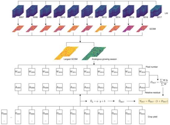
Figure 2.
A schematic process of the forecast of crop yield in an example with Grunty county, Iowa, in 2017. The regional average yield in 2017 was predicted extending the trend line derived from crop yield records during 2000–2016 across the entire region. An analogous growing season to 2017 is identified to have the maximum value of the generic composite similarity measure (GCSM) between time series of leaf area index (LAI) data by pixel. The total number of pixels for each analogous year, which are denoted by W, are determined for the past 10 years. The relative residual D in 2017 is determined to be the weighted average of the relative residuals in the analogous years, which is denoted by . The crop yield Y is finally forecasted by combing the estimated values of regional average and relative residual.
The generic composite similarity measure (GCSM) suggested by Liu et al. [38] was used to assess the similarity of the LAI time series in different years (see Supplementary Information 2). For a simple assessment of similarity between LAI time series data, a correlation analysis can be performed. However, the GCSM allows for a thorough assessment of the similarity between two sets of time series data. For example, the GCSM values are determined by the difference of central tendency and dispersion as well as the strength of correlation between two data sets. The GCSM between two sets of LAI time series was determined between the current year y and a previous year p as follows:
where Ly and Lp indicate the time series of LAI in y and p, respectively. The GCSM value was determined for each pixel of the satellite data. The value of s1 was determined as follows:
where max and min refer to the global maximum and minimum, respectively. The values of max and min were set to be the largest and the smallest values, respectively, within all the time series data, i.e., both Ly and Lp with the average of a given time series data L. The s3 value, which is equivalent to the correlation coefficient between Ly and Lp, was calculated as follows:
where represents standard deviation of a time series L. The s2 value was used to quantify the agreement between the values of standard deviation for L as follows:
A large value of GCSM represents a high degree of similarity between two LAI time series. The maximum value, which is 1, would be obtained if and only if these times series data are identical.
The relative residual of crop yield for a county was determined using the weighted average of the residual values observed in the previous growing seasons for each crop (Figure 2). For each pixel in the given county c, a value of was set to be the analogous year to y when the value of GCSM in p was greater than that of GCSM in any other years for the given period. The number of pixels where an analogous year was p were counted and denoted by Wc,p. The relative residual for the growing season of interest Dc,y was determined as follows:
For example, suppose the analogous years for 2020 were identified to be 2018 and 2019 at 200 and 300 pixels in a given county G, respectively. Then, the value of DG,2020 was determined to be sum of 200/500· and 300/500·.
2.5. Forecast of Crop Yield
The crop yield at the county level was determined combining the values of the trend and the relative residual for soybean and maize, respectively. The crop yield Yc,y was predicted as follows:
where represents the regional average crop yield in year y. The value of was determined in each year using the trend line of crop yield for each crop.
The predicted values of crop yield were classified into two groups. The trend line was derived using the crop yield data from 2000–2016. As a result, no true forecast of crop yield was made for the given period due to information leakage. In the present study, the prediction data for the earlier periods, e.g., 2010–2016, were used to identify the date of crop yield forecast applicable to the region of interest. These data were also used to examine consistency of the prediction data in the given region. In contrast, no crop yield data for the period from 2017–2019 were used for calculation of the regional yield trend. Thus, the prediction data for the later period, e.g., 2017–2019, were assumed to represent true crop yield forecasts and analyzed in more detail including the spatial distribution of errors. The counties where there were less than 30 total cropland pixels were excluded from the analysis of crop yield forecasts. In addition, individual pixels with large uncertainties, which were identified using the quality index values of the LAI data, were removed for the computation of the crop yield.
An R (version 4.0.3) script was written to perform the prediction procedures using the rgee package [39]. A customized script was written to process the satellite data, e.g., MOD15A2H and MCD12Q1, and compute the GCSM values using the Google Earth Engine, which is a cloud-based computing platform [40].
2.6. Error Assessment of Crop Yield Forecasts
The prediction errors of relative residual and crop yield were examined for the period from 2010 to 2016. The mean absolute error (MAE) of the relative residual in a year of interest was determined for the entire region as follows:
where N indicates the number of counties in the study region. and represent observed and predicted relative residuals in county c in the given year y, respectively. The mean absolute percentage error (MAPE) of the crop yield prediction in y was also calculated as follows:
where and are observed and predicted crop yield in c, respectively.
The error of crop yield prediction for the period from 2010–2016 was examined with respect to the duration of the LAI time series. The value of MAPE was determined for each time series of LAI in a given pair of years, which differed by the value of the last date, LD. The MAPE values by the last date were used to infer the reasonable range of lead-time for crop yield forecast.
The errors of crop yield forecast were analyzed for the period from 2017 to 2019 by county. Crop yield data in these recent years had not been used to derive the regional trend of yield. Thus, the analysis of forecast errors in the given growing seasons would provide reliable information on the accuracy of the ABC approach. The LAI time series L [89, 209] was used to forecast crop yields in these years. The DOY 209 was chosen to be the last date for the time series because it was the earliest date in the state-level assessments of crop yield from NASS [41,42].
For each year of forecast, observed and predicted crop yield were compared by county. The percentage error (PE) was calculated for each county to assess spatial distribution of errors as follows:
The root mean squared error (RMSE) was also determined for the entire region as follows:
To our best knowledge, Khaki et al. [12] reported an approach to predict crop yield for the same region of interest in the present study. Their approach had considerably low errors most likely due to its dependency on a sophisticated method and a large quantity of data, e.g., deep neural networks and environmental data. Those error statistics for the ABC method were compared with the ones reported in the previous study to examine if crop yield could be predicted with reasonable accuracy using the simple approach.
3. Results
3.1. The Relative Residuals Predicted Using GCSM
The similarity index values averaged by county tended to be high in the region of interest (see Supplementary Information 3). For example, the average values of GCSM were >0.8 for the time series from DOY 89 to 209 or L [89, 209] except for the growing seasons in 2012 and 2013. The variation in the similarity index was also relatively small across counties in the study region. For example, the coefficient of variation of the GCSM values ranged from 8.3% to 10.5% for the period from 2010 to 2016 except for 2012.
The predicted values of the relative residuals had small errors in 2010–2016 (Figure 3a,b) while the actual values of the relative residual ranged from −90% to 50% for both crops. The MAE of the predicted values for the relative residuals were about 10% in most years for both crops when L [89, 209] was used to identify the analogous growing season. However, the error of predicted relative residual was relatively large, e.g., >15% in 2012 when the average value of GCSM was low, e.g., 0.749.
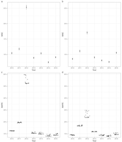
Figure 3.
The errors of the relative residuals and crop yield predicted for (a,c) corn and (b,d) soybean during the period from 2010–2016. The Mean Absolute Error (MAE) was determined for the relative residuals of (a) corn and (b) soybean yield calculated using the LAI time series from the day of year (DOY) of 89 to 209. The point and error bar represent the regional average and the standard error of the relative residuals, respectively. The Mean Absolute Percentage Error (MAPE) was determined for crop yield of (c) corn and (d) soybean for the period from 2010–2016 using the time series of LAI data. The first date of the given time series was set to be DOY of 89. The last date of the time series ranged from DOY of 153 to 305, which created a series of time series data. The dot indicates the MAPE value obtained from each LAI time series.
3.2. Crop Yield Prediction in 2010–2016
Overall, the ABC scheme tended to have small errors of crop yield prediction for the period from 2010 to 2016 except for 2011 and 2012 (Figure 3c,d). The MAPE for both crops ranged from 8% to 15% for the given growing seasons. Still, MAPE for soybean was smaller than that for corn especially in 2012. The magnitude of errors in prediction of crop yield had a relatively small variation for the time series of LAI data. For example, the range of MAPE for all the sets of LAI time series data was about 2% except for the growing season in 2012. Although the variation of MAPE was relatively large in 2012, the difference between maximum and minimum values of the error was about 8% for the given sets of LAI time series.
The ABC approach resulted in small errors of crop yield prediction when a longer time series of LAI was used for the period from 2010–2016 (Figure 4). The LAI time series data with the earlier last date (LD) had the largest values of MAPE on average for the given growing seasons. For example, the MAPE for corn was >19% when L [89, 169] was used for crop yield prediction. However, MAPE decreased as the last date of the LAI time series advanced. The average of MAPE for corn using L [89, 209] was 18%, which was within one standard error of the MAPE values obtained from L [89, 225]. For soybean, the error tended to be smaller than that for corn although the last date for the time series was comparatively later in the growing season such that relatively small errors of crop yield occurred. For example, the MAPE of soybean yield using L [89, 233] was within one standard error of the MAPE values for L [89, 265].
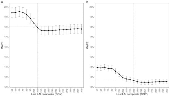
Figure 4.
The MAPE of the estimates of (a) corn and (b) soybean yield in 2010–2016 based on different LAI time series. The first date of LAI time series was set to be the day of year (DOY) of 89. The last date of the time series was set differently from DOY 153–305. The point and error bar indicates the MAPE and the standard error, respectively. The vertical dashed line indicates the earliest DOY when the MAPE was within one standard error of the least one indicated by the horizontal dashed line.
3.3. Crop Yield Forecasts in 2017–2019
The values of GCSM were relatively high in the majority of counties when the LAI time series L [89, 209] in 2017–2019 was used for prediction of crop yield (see Supplementary Information 4). The average GCSM in each county ranged from 0.465 to 0.931 for all three years. The GCSM values were >0.7 in a large number of counties in the study region. However, the value of GCSM tended to be low in states, e.g., Kansas and Missouri, where the cropland acreage was relatively small.
Overall, the use of L [89, 209] resulted in small errors in crop yield forecasts from 2017 to 2019 (Figure 5). The RMSE values for both corn and soybean were within 10% of crop yield recorded in each year. For example, the RMSE for corn ranged from 974.80 to 1121.93 kg ha−1 on average across the region. The correlation coefficients between observed and forecasted crop yield were also high, e.g., >0.85 for both crops.

Figure 5.
Comparisons between county-level yield reports and forecasts of (a–c) corn and (d–f) soybean yields in (a,d) 2017, (b,e) 2018 and (c,f) 2019. The crop yield forecasts were obtained using the LAI time series from the day of year of 89 to 209. The crop yield data were obtained from USDA-NASS.
Small errors of crop yield forecasts were obtained from 2017 to 2019 in the major crop production counties in the Midwestern U.S. (Figure 6). For example, the PE was within in about 70% of counties for both crops. Relatively large errors mainly occurred in states where croplands were sparsely distributed including Kansas, Missouri and North Dakota.
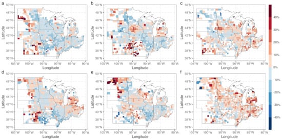
Figure 6.
The percentage error of crop yield forecasts by county. Yield of (a–c) corn and (d–f) soybean was predicted in (a,d) 2017, (b,e) 2018 and (c,f) 2019 using the LAI time series from the day of year of 89 to 209.
4. Discussion
Our results demonstrated that the assessment of similarity between annual crop growth patterns resulted in accurate prediction of crop yield. This analogy-based crop-yield (ABC) prediction approach depends on the assumption that the knowledge of crop growth patterns in the past would allow for accurate prediction of crop yield. Empirical approaches such as deep neural networks and other machine learning methods are based on exactly the same assumption. Still, our approach depends on the crop yield reports in analogous growing seasons for computation of crop yield. These crop yield data would represent realization of a specific set of environment and management conditions in the region of interest for the given growing season. This requires no prediction of the processes involved in crop growth and yield formation, which allows for the minimum use of data for a crop yield forecast. Furthermore, the ABC scheme had low errors in crop yield prediction comparable to a sophisticated neural network model although a single set of satellite data product was used (see Supplementary Information 5). For example, Khaki et al. [12] reported that a crop yield prediction model based on convolutional and recurrent neural networks had RMSE of 1107.26 kg ha−1 and 330.20 kg ha−1 in yield prediction of corn and soybean in 2018, respectively. In the present study, the RMSE of crop yield forecasts for the ABC scheme was 1121.93 kg ha−1 and 329.93 kg ha−1 for the corresponding crops in the same year, respectively.
It was found that the ABC scheme facilitated prediction of crop yield with a reasonable lead time. For example, the errors of crop yield prediction were relatively consistent when LAI data on DOY of 209 were included within the time series data for assessment of similarity between current and previous growing seasons. The LAI often reached a maximum or peak value in late July and early August, e.g., DOY 201–225, in the study region. When the LAI reaches the peak, canopy photosynthesis is at or close to a maximum rate, which provides the source for carbon assimilation for the reproductive growth stages, which is critical for yield formation. Jiang et al. [43] proposed a long short-term memory model of crop growth status to estimate corn yield in the Corn Belt of the U.S., which showed that the phase from silking to dough had the largest contribution to yield estimation. The ABC approach also made the best use of this memory for reasonable prediction of crop yield as early as DOY 209, which provided a lead time of a couple of months (see Supplementary Information 6).
Our results indicated that the errors of crop yield forecast were relatively low in regions where the acreage of crop is relatively large. For example, the PE values of crop yield forecast tended to be lower in counties with higher acreage of cropland (see Supplementary Information 7). In contrast, large errors often occurred in a region that had sparser distribution of cropland. It is likely that such error resulted from a mixed pixel effect since the portion of croplands in a pixel tends to be low. This effect would become conspicuous particularly in regions where the field size is usually small.
Waldner et al. [44] reported that the estimation error of grain yield would decrease when the LAI data at higher temporal resolution become available. Similarly, the consistent and frequent observation of MODIS would have allowed for accurate prediction of crop yield using the ABC method. The daily revisit cycle of MODIS permits production of cloud-free composites of LAI [45]. As a result, the 8-day composite data could allow for preparation of a relatively smooth LAI time series, which would be effective to represent the crop growth pattern during a growing season. The current results confirm that the ABC approach was able to detect crop growing seasons that had a similar phenological pattern over time using this satellite product.
It is likely that the use of LAI products at higher spatial and temporal resolutions can reduce forecast errors for crop yield. The recent development of satellite platforms would allow for the use of hyper-temporal data for crop yield prediction. For example, the observation data obtained from the swarms of satellites, which could provide daily global coverage, would become available for prediction of crop yield [46]. For example, satellite product that has spatial resolution of about 30 m recently became available for crop yield prediction. However, the short-term temporal coverage of the latest satellite data would be the major constraint for application of the ABC scheme. Furthermore, it could be challenging to extract the effective LAI time series from the satellite images at a high spatial resolution due to cloud contamination [47,48,49]. Alternatively, data fusion technologies can allow production of LAI time series data at high spatial and temporal resolutions [50,51,52], which merits further improvement of the ABC approach using these data.
One of the key advantages of the ABC scheme is its dependence on the minimum set of data obtained in current and previous growing seasons. Nevertheless, such a feature could make it challenging to predict crop yield under an extreme weather condition. For example, an unprecedented drought event occurred during the growing season in 2012 [53]. As the ABC scheme depends on the similarity of the temporal patterns of LAI in current and previous growing seasons, the similarity index values were lower in 2012 than the other years. As a result, the ABC scheme had considerably large errors of crop yield prediction in the given growing season. Assessment of growing season similarity for a longer-term period can increase the chances of identifying prior season LAI time series data affected by various weather events, which would minimize prediction errors of crop yield in a growing season of interest.
Under drought conditions, heat stress can cause damage to reproductive parts of a crop resulting in pollen sterility and grain weight loss. In contrast, the biomass of vegetative organs may not be affected by heat stress as much as the reproductive ones especially when drought occurs at an early stage of the reproductive stage [54,55]. As the ABC scheme depends on satellite observation data of vegetative parts, e.g., LAI, it would be challenging to predict crop yield loss caused by such drought events. Alternatively, process-based crop growth models have been used to simulate crop growth under specific conditions [56], which could allow for prediction of crop yield under an extreme weather condition. Still, these models usually require a large amount of input data including weather, soil, crop management and crop genotype. In particular, the availability of site-specific data is often limited, which makes it challenging to apply the process-based crop model to prediction of crop yield. Nevertheless, development of new algorithms would be merited to apply the ABC approach to crop growth models for crop yield prediction under the extreme events.
5. Conclusions
A simple analogy-based approach, which was referred to as ABC, was developed for regional crop yield forecast. In the ABC scheme, the temporal yield trend was determined at the regional scale, which represented advances in agricultural technology. The relative residual to the regional trend was determined by county area basis, which indicated a specific condition for crop growth and yield. The relative residual was predicted using a similarity assessment index of the time series data of LAI between current and previous growing seasons. A previous growing season most analogous to a current one was identified by areas of 500 m by 500 m. Crop yield reports in the analogous growing season were used to determine the relative residuals at a county scale. Then, crop yield was determined to be the sum of the regional trend and the relative residuals in a county of interest. The ABC scheme was applied to prediction of corn and soybean yield in the Midwestern U.S. It was found that the ABC method allowed for timely and accurate forecasts of corn and soybean yields although a single set of satellite data, LAI, was used as input. On average, the MAPE for crop yield forecast was less than 10% for corn and soybean in 2017–2019 with the lead time of a couple of months. Such an error was comparable to a sophisticated model based on deep neural networks. It was also found that errors were relatively small in a region where crops of interest were extensively cultivated. These suggest that the ABC scheme would be useful for a crop growth and yield monitoring program, which requires early forecasts of crop yield within a growing season.
Supplementary Materials
The supplementary materials are available online at https://www.mdpi.com/article/10.3390/rs13163069/s1. Figure S1: Derived time series of average LAI over the cropland in the study area during growing seasons since 2000. Note the sudden drops on DOY 217 and 225 of 2000 resulted from the reset of the MODIS instrument are negligible in the present study. Figure S2: Comparison between the similarity measures for synthetic time series data sets. Figure S3: The GCSM values of the LAI time series from the day of year of 89 to 209 between current and previous growing seasons by year. The point and error bar represent the regional average and the standard error, respectively. Figure S4: The average values of GCSM by county. The GCSM values were determined between LAI time series from the day of year of 89 to 209 in (a) 2017, (b) 2018 and (c) 2019 (c) and their analogous growing seasons. Figure S5: Comparisons between state-level yield reports and forecasts from NASS and the ABC method for (a–c) corn and (d–f) soybean yields in (a,d) 2017, (b,e) 2018 and (c,f) 2019. The ABC crop yield forecasts were obtained using the LAI time series from the day of year of 89 to 209. The crop yield data were obtained from USDA-NASS. The NASS forecasts were reported in August of each year. Figure S6: The relationship between the cropland acreage and the absolute percentage error for forecasting corn (a–c) and soybean (d–f) yields in 2017 (a,d), 2018 (b,e), and 2019 (c,f) based on the LAI time series L[89, 209]. The individual data were obtained by county. Table S1: The error statistics of the model for crop yield forecasts in 2018.
Author Contributions
Conceptualization, Y.L. and K.-S.K.; methodology, Y.L. and K.-S.K.; formal analysis, Y.L. and K.-S.K.; writing-original draft preparation, Y.L., J.K. and K.-S.K.; writing-review and editing D.H.F.; funding acquisition: K.-S.K. All authors have read and agreed to the published version of the manuscript.
Funding
This research was funded by the Rural Development Administration, Republic of Korea, “Cooperative Research for Agriculture Science & Technology Development (PJ014755022021)” programs.
Institutional Review Board Statement
Not applicable.
Informed Consent Statement
Not applicable.
Conflicts of Interest
The authors declare no conflict of interest.
References
- Basso, B.; Liu, L. Seasonal crop yield forecast: Methods, applications, and accuracies. In Advances in Agronomy; Elsevier: Amsterdam, The Netherlands, 2019; pp. 201–255. [Google Scholar]
- Dempewolf, J.; Adusei, B.; Becker-Reshef, I.; Hansen, M.; Potapov, P.; Khan, A.; Barker, B. Wheat yield forecasting for Punjab province from vegetation index time series and historic crop statistics. Remote Sens. 2014, 6, 9653–9675. [Google Scholar] [CrossRef] [Green Version]
- Young, L.J. Agricultural crop forecasting for large geographical areas. Annu. Rev. Stat. Appl. 2019, 6, 173–196. [Google Scholar] [CrossRef]
- Johnson, D.M. An assessment of pre- and within-season remotely sensed variables for forecasting corn and soybean yields in the United States. Remote Sens. Environ. 2014, 141, 116–128. [Google Scholar] [CrossRef]
- Johnson, D.M. A comprehensive assessment of the correlations between field crop yields and commonly used MODIS products. Int. J. Appl. Earth Obs. Geoinf. 2016, 52, 65–81. [Google Scholar] [CrossRef] [Green Version]
- Becker-Reshef, I.; Vermote, E.; Lindeman, M.; Justice, C. A generalized regression-based model for forecasting winter wheat yields in Kansas and Ukraine using MODIS data. Remote Sens. Environ. 2010, 114, 1312–1323. [Google Scholar] [CrossRef]
- Kasampalis, D.; Alexandridis, T.; Deva, C.; Challinor, A.; Moshou, D.; Zalidis, G. Contribution of remote sensing on crop models: A review. J. Imaging 2018, 4, 52. [Google Scholar] [CrossRef] [Green Version]
- Weiss, M.; Jacob, F.; Duveiller, G. Remote sensing for agricultural applications: A meta-review. Remote Sens. Environ. 2020, 236, 111402. [Google Scholar] [CrossRef]
- Huete, A.; Didan, K.; Miura, T.; Rodriguez, E.P.; Gao, X.; Ferreira, L.G. Overview of the radiometric and biophysical performance of the MODIS vegetation indices. Remote Sens. Environ. 2002, 83, 195–213. [Google Scholar] [CrossRef]
- Myneni, R.B.; Hoffman, S.; Knyazikhin, Y.; Privette, J.L.; Glassy, J.; Tian, Y.; Wang, Y.; Song, X.; Zhang, Y.; Smith, G.R.; et al. Global products of vegetation leaf area and fraction absorbed PAR from year one of MODIS data. Remote Sens. Environ. 2002, 83, 214–231. [Google Scholar] [CrossRef] [Green Version]
- Fritz, S.; See, L.; Bayas, J.C.L.; Waldner, F.; Jacques, D.; Becker-Reshef, I.; Whitcraft, A.; Baruth, B.; Bonifacio, R.; Crutchfield, J.; et al. A comparison of global agricultural monitoring systems and current gaps. Agric. Syst. 2019, 168, 258–272. [Google Scholar] [CrossRef]
- Khaki, S.; Wang, L.; Archontoulis, S.V. A cnn-rnn framework for crop yield prediction. Front. Plant Sci. 2020, 10. [Google Scholar] [CrossRef]
- Schwalbert, R.; Amado, T.; Nieto, L.; Corassa, G.; Rice, C.; Peralta, N.; Schauberger, B.; Gornott, C.; Ciampitti, I. Mid-season county-level corn yield forecast for US corn belt integrating satellite imagery and weather variables. Crop Sci. 2020, 60, 739–750. [Google Scholar] [CrossRef]
- Rembold, F.; Atzberger, C.; Savin, I.; Rojas, O. Using low resolution satellite imagery for yield prediction and yield anomaly detection. Remote Sens. 2013, 5, 1704–1733. [Google Scholar] [CrossRef] [Green Version]
- Lobell, D.B.; Thau, D.; Seifert, C.; Engle, E.; Little, B. A scalable satellite-based crop yield mapper. Remote Sens. Environ. 2015, 164, 324–333. [Google Scholar] [CrossRef]
- Jin, Z.; Azzari, G.; Lobell, D.B. Improving the accuracy of satellite-based high-resolution yield estimation: A test of multiple scalable approaches. Agric. For. Meteorol. 2017, 247, 207–220. [Google Scholar] [CrossRef]
- Cai, Y.; Guan, K.; Lobell, D.; Potgieter, A.B.; Wang, S.; Peng, J.; Xu, T.; Asseng, S.; Zhang, Y.; You, L.; et al. Integrating satellite and climate data to predict wheat yield in Australia using machine learning approaches. Agric. For. Meteorol. 2019, 274, 144–159. [Google Scholar] [CrossRef]
- Kang, Y.; Ozdogan, M.; Zhu, X.; Ye, Z.; Hain, C.; Anderson, M. Comparative assessment of environmental variables and machine learning algorithms for maize yield prediction in the US Midwest. Environ. Res. Lett. 2020, 15, 064005. [Google Scholar] [CrossRef]
- Huang, J.; Gómez-Dans, J.L.; Huang, H.; Ma, H.; Wu, Q.; Lewis, P.E.; Liang, S.; Chen, Z.; Xue, J.-H.; Wu, Y.; et al. Assimilation of remote sensing into crop growth models: Current status and perspectives. Agric. For. Meteorol. 2019, 276–277, 107609. [Google Scholar] [CrossRef]
- Jin, X.; Kumar, L.; Li, Z.; Feng, H.; Xu, X.; Yang, G.; Wang, J. A review of data assimilation of remote sensing and crop models. Eur. J. Agron. 2018, 92, 141–152. [Google Scholar] [CrossRef]
- Ford, J.D.; Keskitalo, E.C.H.; Smith, T.; Pearce, T.; Berrang-Ford, L.; Duerden, F.; Smit, B. Case study and analogue methodologies in climate change vulnerability research. WIREs Clim. Chang. 2010, 1, 374–392. [Google Scholar] [CrossRef]
- Gommes, R. Non-parametric crop yield forecasting, a didactic case study for Zimbabwe. In Proceedings of the ISPRS Archives XXXVI-8/W48 Workshop Proceedings: Remote Sensing Support to Crop Yield Forecast and Area Estimates, Stresa, Italy, 30 November–1 December 2006; pp. 79–84. [Google Scholar]
- López-Lozano, R.; Duveiller, G.; Seguini, L.; Meroni, M.; García-Condado, S.; Hooker, J.; Leo, O.; Baruth, B. Towards regional grain yield forecasting with 1 km-resolution EO biophysical products: Strengths and limitations at pan-European level. Agric. For. Meteorol. 2015, 206, 12–32. [Google Scholar] [CrossRef]
- Shao, Y.; Campbell, J.B.; Taff, G.N.; Zheng, B. An analysis of cropland mask choice and ancillary data for annual corn yield forecasting using MODIS data. Int. J. Appl. Earth Obs. Geoinf. 2015, 38, 78–87. [Google Scholar] [CrossRef]
- Yang, L.; Jin, S.; Danielson, P.; Homer, C.; Gass, L.; Bender, S.M.; Case, A.; Costello, C.; Dewitz, J.; Fry, J.; et al. A new generation of the United States national land cover database: Requirements, research priorities, design, and implementation strategies. ISPRS J. Photogramm. Remote Sens. 2018, 146, 108–123. [Google Scholar] [CrossRef]
- Cruze, N.B.; Erciulescu, A.L.; Nandram, B.; Barboza, W.J.; Young, L.J. Producing official county-level agricultural estimates in the United States: Needs and challenges. Stat. Sci. 2019, 34, 301–316. [Google Scholar] [CrossRef]
- Myneni, R.; Knyazikhin, Y.; Park, T. MOD15A2H MODIS/Terra Leaf Area Index/FPAR 8-Day L4 Global 500m SIN Grid V006; NASA EOSDIS Land Processes DAAC: Sioux Falls, SD, USA, 2015. [CrossRef]
- Wang, Q.; Tenhunen, J.; Dinh, N.Q.; Richstein, M.; Otieno, D.; Granier, A.; Pilegarrd, K. Evaluation of seasonal variation of MODIS derived leaf area index at two european deciduous broadleaf forest sites. Remote Sens. Environ. 2005, 96, 475–484. [Google Scholar] [CrossRef]
- Yan, K.; Park, T.; Yan, G.; Chen, C.; Yang, B.; Liu, Z.; Nemani, R.; Knyazikhin, Y.; Myneni, R. Evaluation of MODIS LAI/FPAR product collection 6. Part 1: Consistency and improvements. Remote Sens. 2016, 8, 359. [Google Scholar] [CrossRef] [Green Version]
- Homer, C.; Dewitz, J.; Jin, S.; Xian, G.; Costello, C.; Danielson, P.; Gass, L.; Funk, M.; Wickham, J.; Stehman, S.; et al. Conterminous United States land cover change patterns 2001–2016 from the 2016 national land cover database. ISPRS J. Photogramm. Remote Sens. 2020, 162, 184–199. [Google Scholar] [CrossRef]
- Shao, Y.; Taff, G.N.; Ren, J.; Campbell, J.B. Characterizing major agricultural land change trends in the Western Corn Belt. ISPRS J. Photogramm. Remote Sens. 2016, 122, 116–125. [Google Scholar] [CrossRef] [Green Version]
- Liu, J.; Shang, J.; Qian, B.; Huffman, T.; Zhang, Y.; Dong, T.; Jing, Q.; Martin, T. Crop yield estimation using time-series MODIS data and the effects of cropland masks in Ontario, Canada. Remote Sens. 2019, 11, 2419. [Google Scholar] [CrossRef] [Green Version]
- Wang, X.; Huang, J.; Feng, Q.; Yin, D. Winter wheat yield prediction at county level and uncertainty analysis in main wheat-producing regions of China with deep learning approaches. Remote Sens. 2020, 12, 1744. [Google Scholar] [CrossRef]
- Friedl, D.S.-M. MCD12Q1 MODIS/Terra+Aqua Land Cover Type Yearly L3 Global 500m SIN Grid V006; NASA EOSDIS Land Processes DAAC: Sioux Falls, SD, USA, 2015. [Google Scholar] [CrossRef]
- Bussay, A.; van der Velde, M.; Fumagalli, D.; Seguini, L. Improving operational maize yield forecasting in Hungary. Agric. Syst. 2015, 141, 94–106. [Google Scholar] [CrossRef]
- Lu, J.; Carbone, G.J.; Gao, P. Detrending crop yield data for spatial visualization of drought impacts in the United States, 1895–2014. Agric. For. Meteorol. 2017, 237–238, 196–208. [Google Scholar] [CrossRef]
- Kang, Y.; Özdoğan, M.; Zipper, S.; Román, M.; Walker, J.; Hong, S.; Marshall, M.; Magliulo, V.; Moreno, J.; Alonso, L.; et al. How universal is the relationship between remotely sensed vegetation indices and crop leaf area index? A global assessment. Remote Sens. 2016, 8, 597. [Google Scholar] [CrossRef] [PubMed] [Green Version]
- Liu, Y.; Kim, K.S.; Beresford, R.M.; Fleisher, D.H. A generic composite measure of similarity between geospatial variables. Ecol. Inform. 2020, 60, 101169. [Google Scholar] [CrossRef]
- Aybar, C.; Wu, Q.; Bautista, L.; Yali, R.; Barja, A. Rgee: An R package for interacting with Google Earth Engine. J. Open Source Softw. 2020, 5, 2272. [Google Scholar] [CrossRef]
- Gorelick, N.; Hancher, M.; Dixon, M.; Ilyushchenko, S.; Thau, D.; Moore, R. Google Earth Engine: Planetary-scale geospatial analysis for everyone. Remote Sens. Environ. 2017, 202, 18–27. [Google Scholar] [CrossRef]
- USDA; NASS. The Yield Forecasting Program of NASS. In SMB Staff Report Number SMB 12-01; 2012. Available online: https://www.nass.usda.gov/Publications/Methodology_and_Data_Quality/Advanced_Topics/Yield%20Forecasting%20Program%20of%20NASS.pdf (accessed on 20 March 2020).
- Sakamoto, T.; Gitelson, A.A.; Arkebauer, T.J. Near real-time prediction of U.S. corn yields based on time-series MODIS data. Remote Sens. Environ. 2014, 147, 219–231. [Google Scholar] [CrossRef]
- Jiang, H.; Hu, H.; Zhong, R.; Xu, J.; Xu, J.; Huang, J.; Wang, S.; Ying, Y.; Lin, T. A deep learning approach to conflating heterogeneous geospatial data for corn yield estimation: A case study of the US Corn Belt at the county level. Glob. Chang. Biol. 2019, 26, 1754–1766. [Google Scholar] [CrossRef]
- Waldner, F.; Horan, H.; Chen, Y.; Hochman, Z. High temporal resolution of leaf area data improves empirical estimation of grain yield. Sci. Rep. 2019, 9. [Google Scholar] [CrossRef] [PubMed] [Green Version]
- Massey, R.; Sankey, T.T.; Congalton, R.G.; Yadav, K.; Thenkabail, P.S.; Ozdogan, M.; Meador, A.J.S. MODIS phenology-derived, multi-year distribution of conterminous U.S. crop types. Remote Sens. Environ. 2017, 198, 490–503. [Google Scholar] [CrossRef]
- Butler, D. Many eyes on Earth. Nature 2014, 505, 143–144. [Google Scholar] [CrossRef]
- Onojeghuo, A.O.; Blackburn, G.A.; Wang, Q.; Atkinson, P.M.; Kindred, D.; Miao, Y. Rice crop phenology mapping at high spatial and temporal resolution using downscaled MODIS time-series. GISci. Remote Sens. 2018, 55, 659–677. [Google Scholar] [CrossRef] [Green Version]
- Pan, Z.; Huang, J.; Zhou, Q.; Wang, L.; Cheng, Y.; Zhang, H.; Blackburn, G.A.; Yan, J.; Liu, J. Mapping crop phenology using NDVI time-series derived from HJ-1 A/B data. Int. J. Appl. Earth Obs. Geoinf. 2015, 34, 188–197. [Google Scholar] [CrossRef] [Green Version]
- Wulder, M.A.; Loveland, T.R.; Roy, D.P.; Crawford, C.J.; Masek, J.G.; Woodcock, C.E.; Allen, R.G.; Anderson, M.C.; Belward, A.S.; Cohen, W.B.; et al. Current status of Landsat program, science, and applications. Remote Sens. Environ. 2019, 225, 127–147. [Google Scholar] [CrossRef]
- Battude, M.; Bitar, A.A.; Morin, D.; Cros, J.; Huc, M.; Sicre, C.M.; Dantec, V.L.; Demarez, V. Estimating maize biomass and yield over large areas using high spatial and temporal resolution Sentinel-2 like remote sensing data. Remote Sens. Environ. 2016, 184, 668–681. [Google Scholar] [CrossRef]
- Gao, F.; Anderson, M.C.; Zhang, X.; Yang, Z.; Alfieri, J.G.; Kustas, W.P.; Mueller, R.; Johnson, D.M.; Prueger, J.H. Toward mapping crop progress at field scales through fusion of Landsat and MODIS imagery. Remote Sens. Environ. 2017, 188, 9–25. [Google Scholar] [CrossRef] [Green Version]
- He, M.; Kimball, J.; Maneta, M.; Maxwell, B.; Moreno, A.; Beguería, S.; Wu, X. Regional crop gross primary productivity and yield estimation using fused Landsat-MODIS data. Remote Sens. 2018, 10, 372. [Google Scholar] [CrossRef] [Green Version]
- Rippey, B.R. The U.S. drought of 2012. Weather Clim. Extrem. 2015, 10, 57–64. [Google Scholar] [CrossRef] [Green Version]
- Ruiz-Vera, U.M.; Siebers, M.H.; Drag, D.W.; Ort, D.R.; Bernacchi, C.J. Canopy warming caused photosynthetic acclimation and reduced seed yield in maize grown at ambient and elevated [CO2]. Glob. Chang. Biol. 2015, 21, 4237–4249. [Google Scholar] [CrossRef] [PubMed]
- Siebers, M.H.; Slattery, R.A.; Yendrek, C.R.; Locke, A.M.; Drag, D.; Ainsworth, E.A.; Bernacchi, C.J.; Ort, D.R. Simulated heat waves during maize reproductive stages alter reproductive growth but have no lasting effect when applied during vegetative stages. Agric. Ecosyst. Environ. 2017, 240, 162–170. [Google Scholar] [CrossRef] [Green Version]
- Hoogenboom, G.; Porter, C.H.; Boote, K.J.; Shelia, V.; Wilkens, P.W.; Singh, U.; White, J.W.; Asseng, S.; Lizaso, J.I.; Moreno, L.P.; et al. The DSSAT crop modeling ecosystem. In Advances in Crop Modelling for a Sustainable Agriculture; Burleigh Dodds Science Publishing: Cambridge, UK, 2019; pp. 173–216. [Google Scholar]
Publisher’s Note: MDPI stays neutral with regard to jurisdictional claims in published maps and institutional affiliations. |
© 2021 by the authors. Licensee MDPI, Basel, Switzerland. This article is an open access article distributed under the terms and conditions of the Creative Commons Attribution (CC BY) license (https://creativecommons.org/licenses/by/4.0/).