Abstract
Convenient, efficient, and high-throughput estimation of wheat heading dates is of great significance in plant sciences and agricultural research. However, documenting heading dates is time-consuming, labor-intensive, and subjective on a large-scale field. To overcome these challenges, model- and image-based approaches are used to estimate heading dates. Phenology models usually require complicated parameters calibrations, making it difficult to model other varieties and different locations, while in situ field-image recognition usually requires the deployment of a large amount of observational equipment, which is expensive. Therefore, in this study, we proposed a growth curve-based method for estimating wheat heading dates. The method first generates a height-based continuous growth curve based on five time-series unmanned aerial vehicle (UAV) images captured over the entire wheat growth cycle (>200 d). Then estimate the heading date by generated growth curve. As a result, the proposed method had a mean absolute error of 2.81 d and a root mean square error of 3.49 d for 72 wheat plots composed of different varieties and densities sown on different dates. Thus, the proposed method is straightforward, efficient, and affordable and meets the high-throughput estimation requirements of large-scale fields and underdeveloped areas.
1. Introduction
Climate change affects agriculture and food production in complex ways [1]. It is estimated that double the present rate of crop production will be needed to meet the needs of the growing population globally by 2050 [2]. The rapid increase in global food production over the past 60 years has been one of the greatest public health achievements in modern history, partly because of technological innovations, including the development of high-yielding crop varieties, production and use of chemical fertilizers and pesticides, as well as agricultural mechanization [3]. Although global food production has increased rapidly, a significant component of the population remains undernourished. Two billion individuals experience micronutrient malnutrition; 161 million children under 5 years of age are stunted, 51 million are wasted, and 794 million individuals are estimated to be calorie deficient [4]. Therefore, identifying and monitoring the phenological stages of crops is essential for breeding new varieties, selecting dominant species, and determining reasonable cultivation methods and accurate field management strategies (irrigation and fertilization) to improve grain yield and quality and promote food security. The heading stage is one of the most critical periods during wheat growth, which is significantly correlated with final yield [5]. Therefore, efficient and high-throughput observations and recordings of wheat heading dates are of great importance.
The heading date is usually recorded through field observations by agronomists. The observer selects a suitable plant sample from a large field and then visually evaluates the wheat growth period. However, there are several challenges with this approach: (i) field observations are labor-intensive; (ii) the time required for data collection increases with the distance between the observation station and the sampling sites, which are situated at different locations; (iii) interpretations of observation criteria increase human error; and (iv) frequent observations are required to evaluate the transition time to a new stage, which can damage crops and the growing environment. Therefore, an automatic, continuous, and non-destructive crop observation method is required [6].
Phenological model-based approaches provide another way to estimate the heading dates of crops. Kawakita et al. developed three winter wheat phenology models with different structures, namely the Agricultural Production System Simulator Model for wheat, the Wang and Engel model, and the model based on sigmoid and exponential functions [7]. These models were calibrated using three parameterization methods to predict wheat heading dates: augmented Lagrange multiplier method, Nelder–Mead method, and Bayesian optimization with Gaussian process. Six-fold cross-validation of nine combinations of model calibration (three models × three parameterizations) showed that the accuracy of the root mean square error (RMSE) ranged from 2 to 7 d [7]. Furthermore, Velumani et al. parameterized models for nine wheat varieties based on daily temperatures, vernalization, and photoperiod characteristics observed in the field experiments for four years (2016–2019). The RMSE and the mean absolute error (MAE) using the calibrated ARCWHEAT crop model were 4.24 d and 3.11 d, respectively [8]. Although crop phenology models can be used to predict the heading dates of wheat and other crops at an early stage, model calibration for each species is time-consuming, requires periodic observations throughout the crop growth cycle (including cumulated temperature, vernalization, and photoperiod), and needs replicates at multiple locations over many years [8]. Additionally, the differences in model structure and parameterization methods cause parametric and predictive uncertainties, limiting the widespread use of phenological models [7].
Previous studies also have proven that ear detection based on digital images can be used to estimate heading dates. Zhu et al. proposed a two-step coarse-to-fine wheat ear detection method. Subsequently, the estimation of the heading date was based on the number of wheat ears, and an MAE of 1.14 d was reported [9]. Similarly, Bai et al. used a new multi-classifier cascade method for rice ear detection, whose numbers were used to evaluate the heading dates. The difference between the proposed multi-classifier cascade method and the manual method was 2 d [10]. These methods accurately estimated the heading dates by detecting wheat or rice ears based on image recognition. However, both studies used empirical thresholds (i.e., number of spikes) to determine the heading dates, with Zhu et al. using the number of spikes in patches as a threshold in an a priori dataset and Bai et al. directly calibrating the threshold at 200, which may vary depending on the variety and the study area. Desai et al. proposed a simple method to detect candidate rice ear regions using red-green-blue (RGB) images, which were used to estimate the heading dates for five datasets containing three different rice varieties with an MAE of <1 d using convolutional neural network-based image classification [11]. In comparison, Velumani et al. proposed an automatic method based on a series of RGB images captured daily using an RGB camera fixed in the field. In this method, the convolutional neural network recognized the presence or absence of wheat ears in small plots, and the heading dates were then estimated based on the ear dynamics observed in the images over time. The method was extensively applied and validated over three years at 47 test sites and nine wheat varieties in different regions of France. Moreover, with an RMSE of approximately 2 d, the method outperformed the ARCWHEAT crop model calibrated to local conditions [8]. Similarly, Wang et al. used digital images captured using a mobile vehicle-mounted DSLR camera to detect the wheat heading rate and combined it with a logistic curve to estimate wheat heading dates, with an MAE and RMSE of 0.99 d and 1.25 d, respectively [12]. Model- and image-based approaches help record heading dates for breeding and cultivation experiments that require a lot of plots [13].
Rapid advances in unmanned aerial vehicle (UAV) technology have been applied to many areas of agricultural research, including estimation of plant height with the RMSE of 0.02–0.07 m using digital surface model (DSM) [14], estimation of canopy cover with a determination coefficient R2 = 0.99 using a decision-tree-based segmentation model [15,16], estimation of canopy temperature using a miniature longwave infrared camera [17], evaluating the water status of soybean plants via thermal images [18], estimation of leaf chlorophyll content using a hyperspectral line scanner and random forest models [19], estimation of nitrogen content using multispectral data [20], estimation of biomass with an R² = 0.71 using DSM [21], and estimation of soybean and potato yield using RGB, multispectral, hyperspectral, and thermal data [22,23], identification of pests and diseases of potato using object-based image analysis method and random forest model [24], and cotton seedling detection and counting with an R² = 0.98 using a deep-learning-based approach [25]. Furthermore, previous studies on crop characteristics have used UAV images to fit sigmoid functions to simulate crop growth. Borra-Serrano et al. used beta and Gompertz functions to fit canopy cover and canopy height, which were then used to calculate crop parameters, including maximum absolute growth rate, early vigor, maximum height, and senescence for different genotypes of soybean [26]. In addition, Chang et al. compared the sorghum canopy height measured using UAV images and sigmoidal curves with those measured on-site to reveal the efficiency of UAV-based methods [27].
However, few studies have estimated the wheat heading dates using UAV images. Despite a large observational range and high efficiency, it is inconvenient for UAVs to take high-frequency images at the daily level. Therefore, it would be of special interest to determine whether and how UAV-acquired wheat images can be used for heading date estimation when only a few UAV images are available throughout the growth cycle. The overall goal of this research was to develop a high-throughput wheat heading date estimation method over a large area based on UAV images. We monitored wheat canopy cover and height changes using UAV images and fit continuous growth curves using crop growth functions to estimate the heading dates. We also compared the estimated results of nine crop growth curves and three plant height estimation methods and analyzed the causes of errors and possible methods to improve accuracy. It is proven that UAV images can be used to estimate wheat heading dates. We also provide a feasible solution to estimate the wheat heading dates on a large scale.
2. Materials and Methods
2.1. Study Area
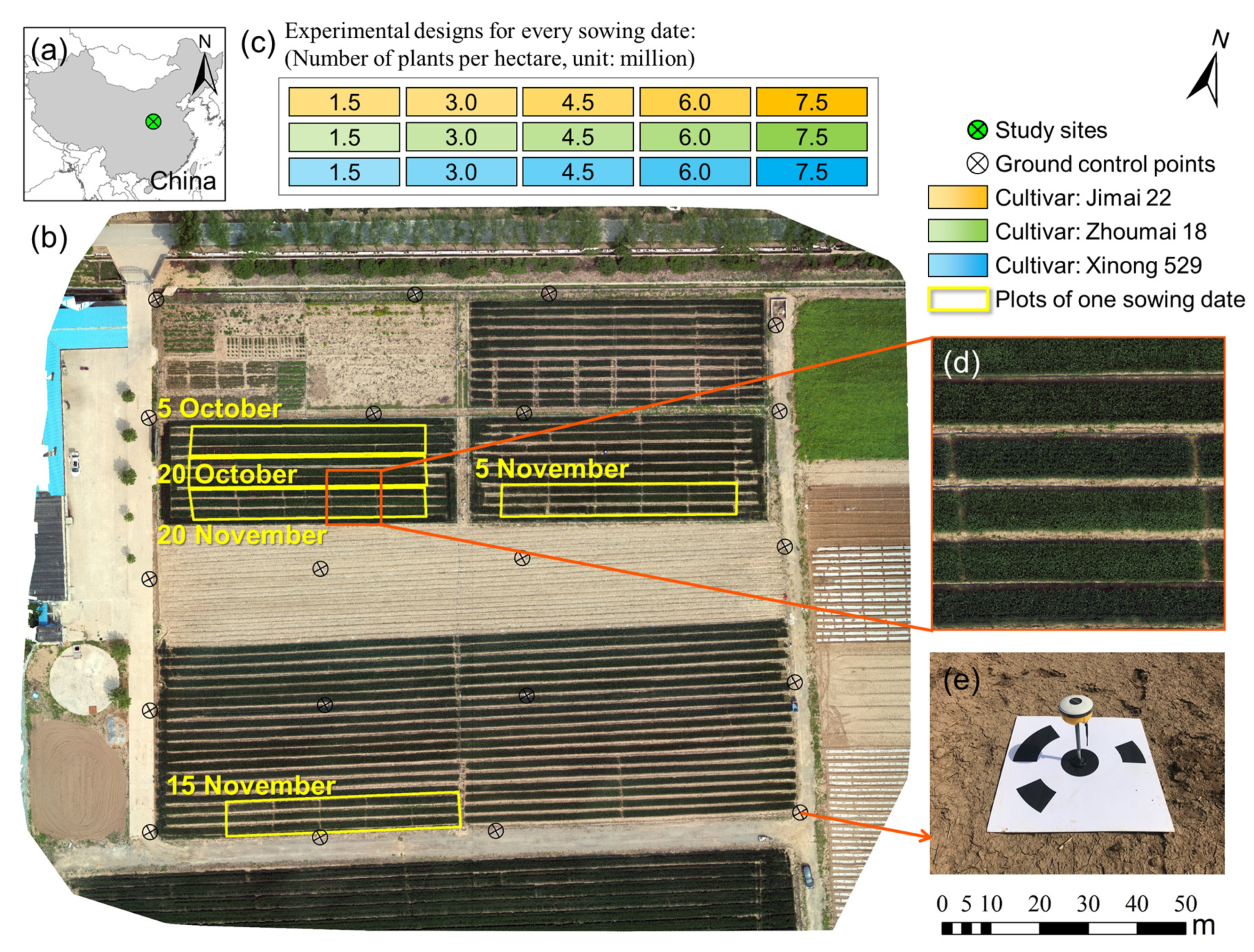
The study site was located at Nanhua Farm of the Institute of Cotton Science, Shanxi Agricultural University, Yuncheng City, central China (34° N 110° E, Figure 1). This site has a temperate continental monsoon climate, and the yearly radiation value of 2019 was 4777.03 MJ/m2 (recorded by the nearest station data of the China Meteorological Radiation Data International Exchange Stations). The average annual rainfall in this region is 559.3 mm, the average annual sunshine duration is 2247.4 h, the annual frost-free period is approximately 208 d, and the average annual and accumulated temperatures are 13.6 °C and 513.8 °C, respectively, which are suitable for the growth of wheat [28].

Figure 1.
Study area and experimental design. (a) Location of the study area; (b) Orthomosaic; (c) Cultivation plots for each sowing date; (d) Magnified image of the orthomosaic; (e) Measurements of a ground control point.
A total of 75 experimental wheat plots, observed from October 2018 to June 2019, were set up using three wheat varieties (Jimai 22, Zhoumai 18, and Xinong 529) sown on five different dates (5 October, 20 October, 5 November, 15 November, and 25 November) with five plant densities (1.5 million, 3 million, 4.5 million, 6 million, and 7.5 million plants/ha) (Figure 1, Table 1). The dimensions of one plot are about 1.15 m × 9 m (10.35 m2).

Table 1.
Plot designs for field experiments and heading date records.
2.2. Data Collection
Field images were captured using a DJI Phantom 4 Advanced UAV (DJI Innovations, Shenzhen, China) with a 1-inch 20-megapixel image (RGB) sensor on 6 March, 28 March, 24 April, 21 May, and 6 June, when the weather was clear. The field data were collected with the lens shooting vertically downward and the flight altitude set to 30 m. The interval for taking pictures was 2 s/image, the heading and side overlap rates were >60% and >80%, respectively, and the sizes of the acquired images were 5472 × 3648 and 5472 × 3078 in the JPG format for 6 March and other sowing dates, respectively (Table 2). The spatial resolutions of the orthomosaic and DSM are shown in Table 2. A slightly larger resolution was used on 6 March than those on the other dates at the same flight altitude owing to the larger image size setting of the UAV.

Table 2.
UAV data (orthomosaic and digital surface model) information.
Real-time kinematic GNSS (Unistrong Industrial Co. Ltd., Beijing, China) and positioning service (Qianxun SI, Shanghai, China) with centimeter-level accuracy (<10 cm) were used to measure the geographical locations of the ground control points (GCPs) before UAV data acquisition (Figure 1e). The GCPs were evenly distributed in the study area, with 15–22 GCPs at each time (Table 2).
2.3. Determination of Heading Date
According to the definition of heading date [29], i.e., approximately 50% of the stalks are expected to have ears after entering the heading stage; the heading stage was observed daily by two agronomists and the heading dates were recorded for 75 experimental plots (Table 1).
2.4. Canopy Coverage Estimation
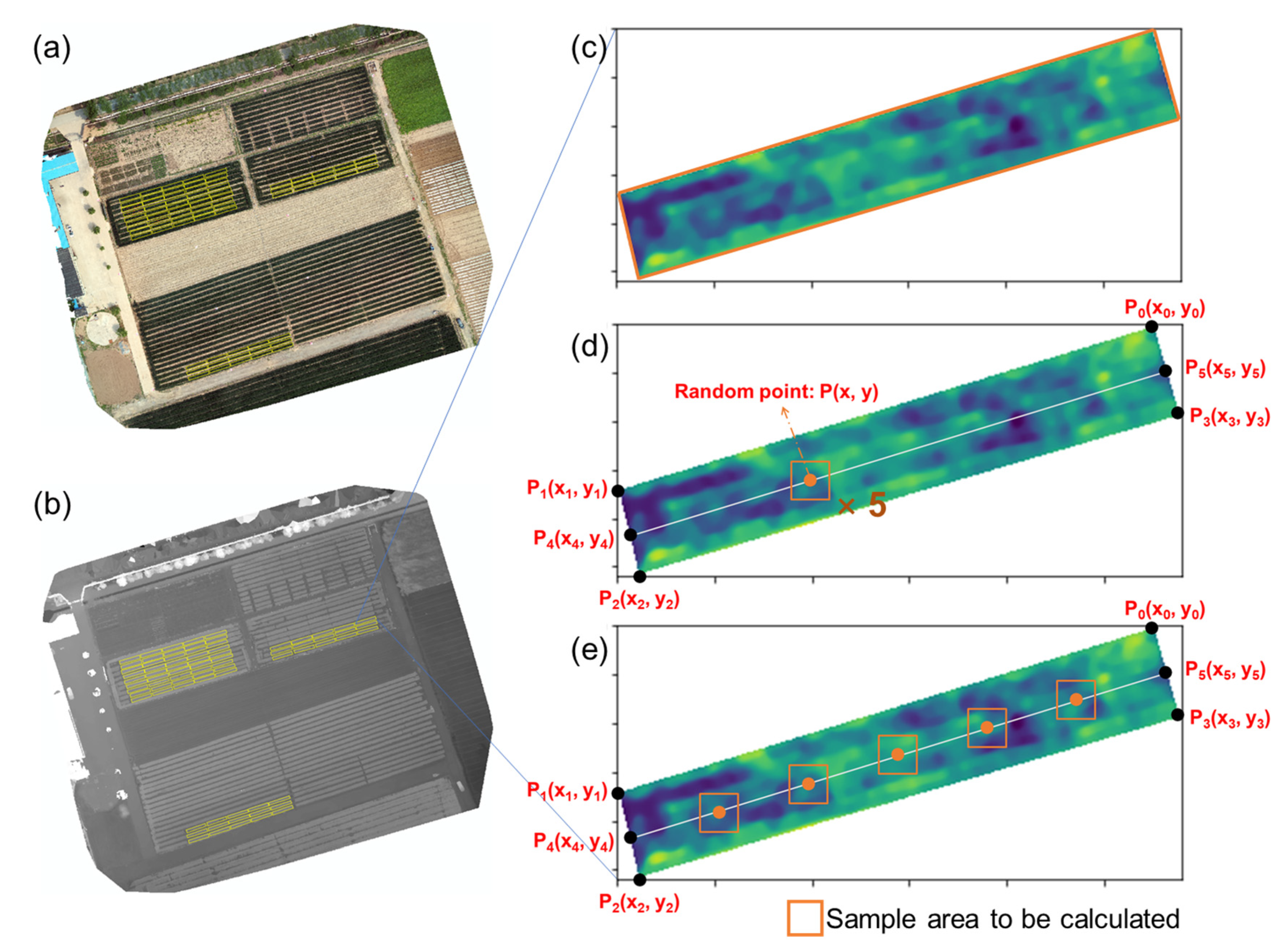
The training sample files were generated in *.csv format using collectTrainJS_v2 software to divide the farmland into positive samples (wheat) and negative samples (others) [15]. The training samples have nine features composed of red (R), green (G), blue (B), lightness (L), color-opponent dimensions (a and b), hue (H), saturation (S), and valve (V). The EasyIDP package of Python was used to calculate the median axis in the raw UAV images of each plot [30]. Support vector machine method has been proved to be a powerful tool for problems of classification, regression for many previous studies [9,10]. Support vector machine use nonlinear functions to map the original feature to a higher-dimensional space and find hypersurfaces that can divide the positive samples (wheat) and negative samples (others). Five equal interval sampling strategies were implemented along the central axis (Figure 2e), and a trained support vector machine model was used for each sample to calculate canopy coverage by the proportion of wheat pixels to the total pixels [15]. Then the average of each five samples was used as the plot canopy coverage.

Figure 2.
Models and sampling methods used for plant height estimation. (a) Orthomosaic; (b) Digital surface model; (c) Sampling method 1: whole region calculation; (d) Sampling method 2: random sampling; (e) Sampling method 3: equal interval sampling.
2.5. Plant Height Estimation
A DSM was generated using the UAV images of the study area to calculate the wheat plant height, which included two components: UAV image processing and estimating plant height.
2.5.1. UAV Image Processing
Using the Pix4Dmapper software (Pix4D SA, Lausanne, Switzerland), the UAV images were processed, aligned, and matched and dense point clouds, orthomosaic, and DSMs were generated. Additionally, GCPs were included in data processing to obtain geographically accurate orthomosaic and DSMs in Geo-tiff format.
The boundaries (shapefile format, Figure 2a) of the study plot were extracted using ArcGIS 10.2 (ESRI, Redlands, CA, USA) and the orthomosaic of 6 March.
2.5.2. Plant Height Estimation Using UAV Images
Based on the shapefile and time-series DSM files, plot DSM images were cropped using the EasyIDP package of Python [30]. A linear regression model was obtained using the RKT-measured elevations and the corresponding corrected DSM values to further calibrate the DSM value. Wheat plant height was estimated as the difference between the canopy height (95th percentile of the plot DSM) and the ground height (5th percentile of the plot DSM) (Equation (1)). To calculate canopy height, the following sampling methods were used: (1) whole region calculation; (2) random sampling; (3) equal interval sampling.
In the whole region calculation method, all DSM values for the plot (all pixels within P0, P1, P2, and P3, Figure 2c) were ranked and the 95th percentile was used as the canopy height. In random sampling, five random square samples were selected on the plot axis P4, P5, and the length of each sample was calculated as half the length of the shorter side of the plot. Then, the average of the 95th percentile of the five samples was calculated and used as the plot canopy height (Figure 2d). For the equal interval sampling method, five square samples were identified on the central axis, each with a point at its center, which divided the central axis into six equal parts. Thereafter, the 95th percentile of each sample was determined separately as the canopy height (Figure 2e).
where and are the canopy and ground height, respectively.
2.6. Growth Curve Fitting
2.6.1. Sigmoidal Curve
Nine sigmoidal functions were selected to fit the wheat growth curves based on plant height and canopy coverage obtained from the UAV data collected during the wheat growth period (Equations (2)–(9)). The initial phase of model growth was approximately exponential, but the growth rate linearized as saturation began. At maturity, growth completely stopped. This progression was used to model the continuous growth in wheat plant height and the changes in canopy coverage.
where represents the number of days after UAV image acquisition (6 March), is the plant height or canopy coverage, is the initial value, is the final value, and is the rate of change of the curve [31].
where represents the number of days after UAV image acquisition (6 March), is the plant height or canopy coverage, is the maximum value, is the growth rate, and represents the number of days that wheat requires to reach half its final value [8].
where represents the number of days after UAV image acquisition (6 March), represents the crop height or canopy coverage, is the maximum, is the growth rate, and is the half of the final value [27].
where represents the number of days after UAV image acquisition (6 March), is the canopy coverage or plant height, is the maximum value, is the growth rate, and is the inflection point at which the growth rate reaches the maximum [26].
where represents the number of days after UAV image acquisition (6 March), is the plant height or canopy coverage, is the maximum value, is the time required to reach the maximum growth rate, and is the curve parameter [32].
where represents the number of days after UAV image acquisition (6 March), is the plant height or canopy coverage, is the maximum value, is the time corresponding to the maximum value, and is the time required to reach the maximum growth rate [26].
where represents the number of days after UAV image acquisition (6 March), is the plant height or canopy coverage, is the maximum value, and and are curve parameters [33].
where represents the number of days after UAV image acquisition (6 March), is the plant height or canopy coverage, is the maximum value, is the growth rate, and is the initial value [34].
where is the number of days after UAV image acquisition (6 March), is the canopy coverage or plant height, and , , and are curve parameters [12].
2.6.2. Curve Fitting
We used five-time series for wheat plant height and canopy coverage to fit the growth curves and the Scipy package of Python to solve the parameters in Equations (2)–(10) [35]. The continuous plant height and coverage growth curves of wheat were obtained using the fit growth curve models.
2.7. Estimation of Heading Date
The second derivatives of the continuous growth curves of wheat plant height, which represent the acceleration in wheat plant height, were calculated. We then estimated the number of days at which the minimum value of the second derivative was located, based on the curves, to determine the heading date.
2.8. Accuracy Evaluation of the Proposed Model
To evaluate the accuracy of the proposed method, we calculated the error between the estimated values and the field values recorded by the agronomists, along with the maximum and minimum error values, MAE, and RMSE. The smaller the error, the higher the accuracy of the estimation.
where is the heading date recorded by agronomists in the field, is the heading date estimated using wheat plant height, and is the number of plots.
3. Result
3.1. Plant Height Growth Curve
We calculated the plant height of 72 experimental plots (three plots affected by the experimental sampling frame were excluded, Figure 3) of five different UAV images based on the whole region calculation method (Table S2). We used nine sigmoidal functions (Equations (2)–(10)) to fit the growth curves of wheat plant height, calculated their second derivative minima, and compared them with the heading dates recorded in the field (Table 3).
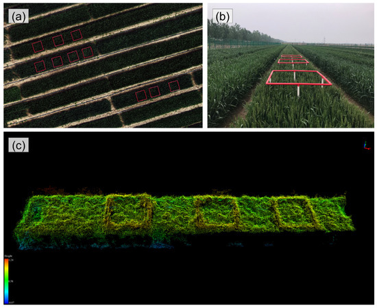
Figure 3.
Plots affected by sample frame. (a) Orthomosaic, (b) side view, (c) dense point cloud of plot (sowing date: 5 October; variety: Xinong 529; density: 1.5 million plants/ha).

Table 3.
Estimated results of nine sigmoidal functions.
The results revealed that Equations (5), (7) and (8) could not fit the growth curves of wheat plant height and could not be used to estimate the wheat heading dates. Equation (3) could only fit the growth curves of plant height in six plots, while Equations (2) and (6) fit the height growth curves of plants in 71 plots, and Equations (9) and (10) fit the growth curves of plants in 70 plots. Equation (4) was the most consistent and fit the growth curves of plant height in all 72 plots to provide accurate wheat heading dates. Moreover, Equations (2), (4), (9) and (10) had similar estimation accuracies. Equations (3) and (6) had lower estimation accuracies, whereas Equations (9) and (10) had the highest estimation accuracies.
3.2. Growth Curves of Canopy Coverage
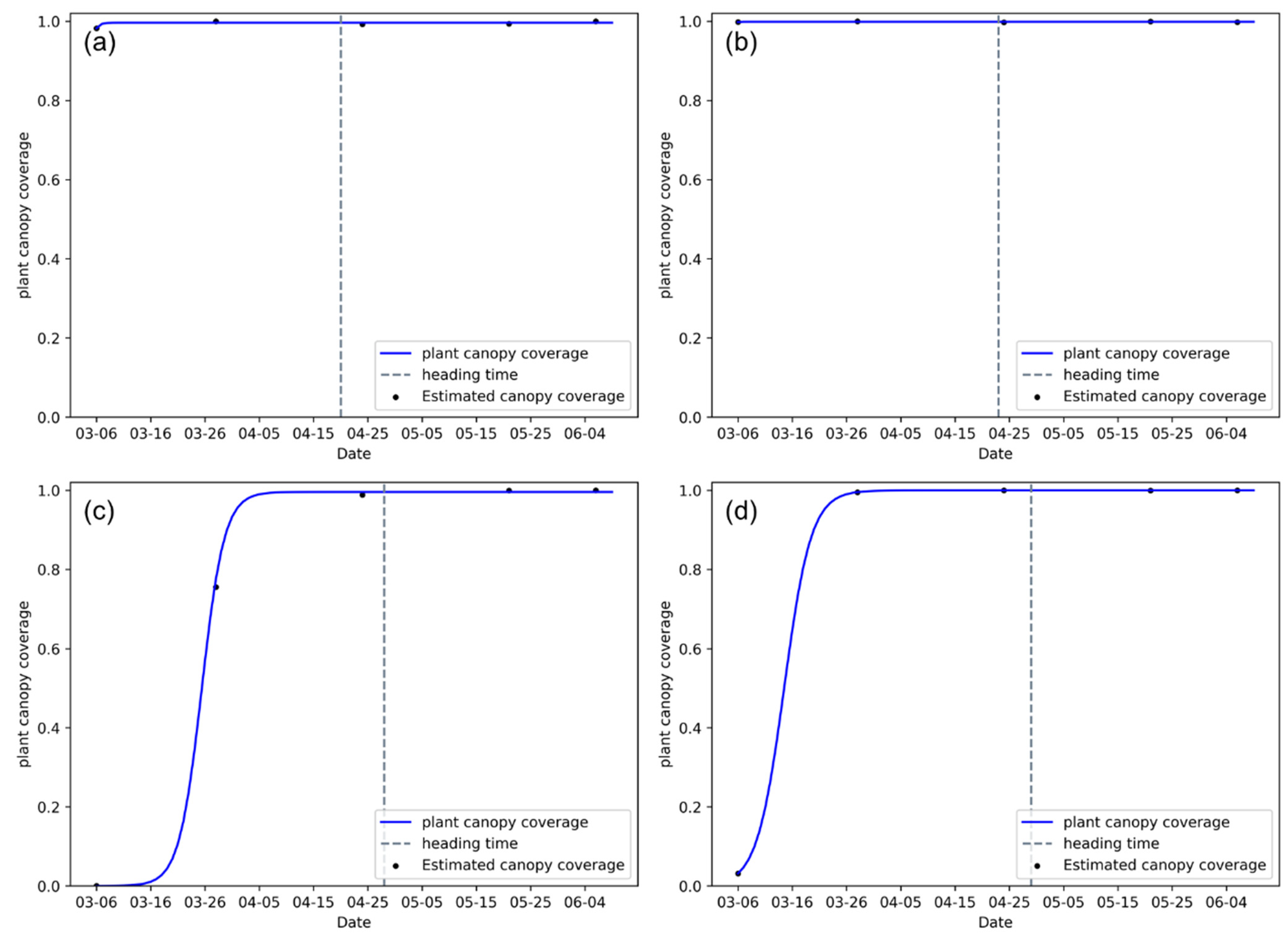
We estimated the wheat canopy coverage of each plot using raw UAV images and fit the canopy coverage growth curves using Equation (4). The growth curves of the 72 plots are shown in Supplementary Material. Figure 4 shows the canopy coverage growth curves for early sowing-low density (sowing date: 5 October; variety: Zhoumai 18; density: 1.5 million plants/ha), early sowing-high density (sowing date: 5 October; variety: Zhoumai 18; density: 7.5 million plants/ha), late sowing-low density (sowing date: 25 November; variety: Zhoumai 18; density: 1.5 million plants/ha), and late sowing-high density (sowing date: 25 November; variety: Zhoumai 18; density: 7.5 million plants/ha) plots, wherein the wheat canopy coverage was saturated at the heading stage, and no apparent changes in wheat canopy coverage were observed. Therefore, it was difficult to estimate the wheat heading dates based on the changes in canopy coverage.
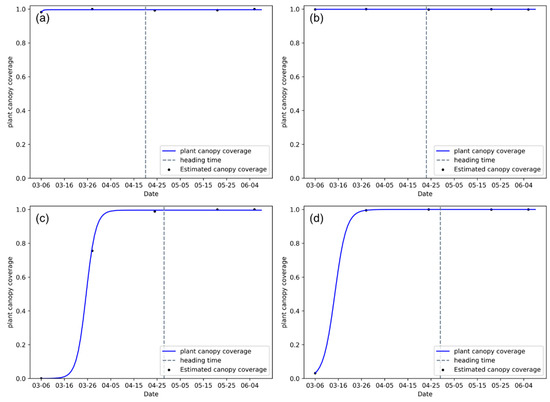
Figure 4.
Canopy coverage growth curve. (a) early sowing-low density plot (sowing date: 5 October; variety: Zhoumai 18; density: 1.5 million plants/ha), (b) early sowing-high density plot (sowing date: 5 October; variety: Zhoumai 18; density: 7.5 million plants/ha), (c) late sowing-low density plot (sowing date: 25 November; variety: Zhoumai 18; density: 1.5 million plants/ha), (d) late sowing-high density plot (sowing date: 25 November; variety: Zhoumai 18; density: 7.5 million plants/ha). Gray dashed line indicates the heading date recorded in the field.
3.3. Sampling Methods of Plant Height Estimation
To calculate plant height from UAV images, the plant height of wheat was obtained using Equation (1). Five linear regression models were obtained using the RKT-measured elevations and the corresponding corrected DSM values to further calibrate the DSM value (Figure S1). However, different sampling methods gave different results, and a large sampling area increased computing cost. Therefore, the random sampling method, which used the average values of five samplings, could reduce computational costs (the sum of calculated pixels number for five samplings is about 1/5 of the whole plot). Furthermore, the equal interval sampling allowed each sample to be used as a separate time series to estimate the heading date, and the heading dates estimated from five samples were averaged to be the estimated heading date for each plot. It is beneficial to reduce the computational costs and consider the crop heterogeneity.
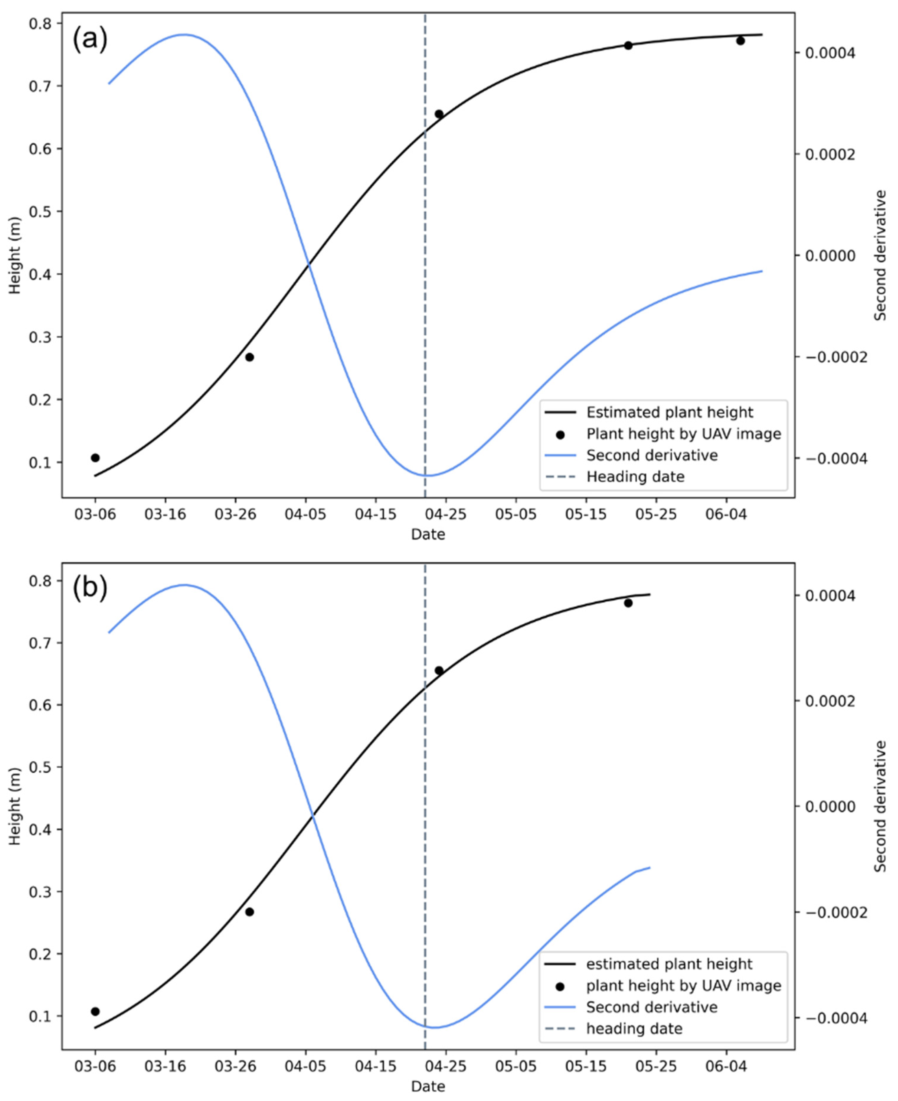
The plant height estimated by the three sampling methods are shown in Tables S2–S8. The growth curves of plant height estimated using UAV images were fit using Equation (4). The growth curves and second derivatives for the minimum error plots (sowing date: 20 October; variety: Xinong 529; density: 1.5 million plants/ha) and maximum error plot (sowing date: 5 November; variety: Zhoumai 18; density: 7.5 million plants/ha) derived using the whole region calculation method are shown in Figure 5, respectively. The growth curves and second derivatives for other plots are shown in Supplementary Materials. The heading dates were calculated using the minima of the second derivatives (Table S9), where the wheat heading date of the equal interval sampling method was estimated by the mean of the heading dates calculated for the five-time series (Table S10).
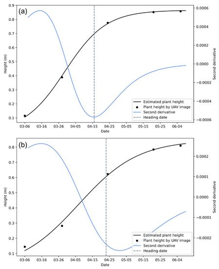
Figure 5.
Figure showing plant height growth curve and the second derivative of the minimum error and maximum error plots derived using the whole region calculation method. (a) the minimum error plot (sowing date: 20 October; variety: Xinong 529; density: 1.5 million plants/ha), (b) the maximum error plot (sowing date: November 5; variety: Zhoumai 18; density: 7.5 million plants/ha). The black dots represent plant height obtained using UAV images, the black curve represents the plant height growth curve, and the gray dashed line represents the observed heading date.
3.4. Evaluation of the Accuracy of the Estimated Heading Dates
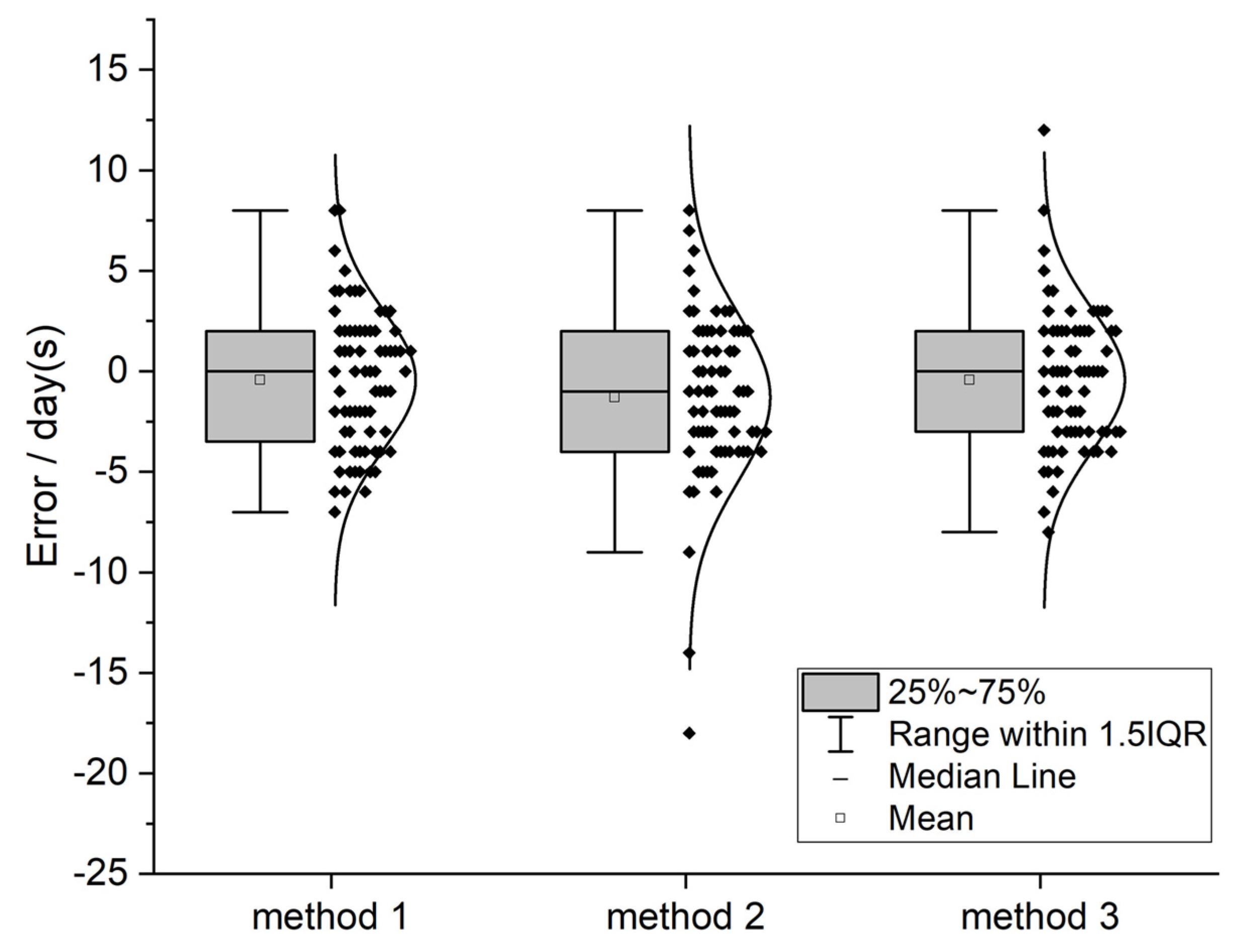
The accuracy of UAV image-based estimates of heading date was evaluated using the field records (Table 4). MAE and RMSE were the maxima for sampling method 2, i.e., the random sampling method. The minimum MAE and RMSE were observed for the equal interval sampling method.

Table 4.
Accuracy of heading dates estimated using UAV images (days).
The error distribution of the three sampling methods is shown in Figure 6. Except for some large errors, most of the estimation errors were within 5 d.
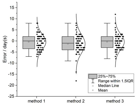
Figure 6.
Box plots showing error distributions of the three sampling methods used to estimate wheat heading dates. IQR: interquartile range.
3.5. Interference in the Field
Among the 75 plots, three plots had square sample frames (height greater than wheat, Figure 3) because of the field experiment requirements. These plots affected plant height estimation and accurate simulation of wheat growth, resulting in erroneous estimates of the heading dates. Thus, to overcome the frame effects in heading date estimation, i.e., to estimate plant height accurately, we manually removed the DSM data of the affected area to calculate the DSM percentile values. The results showed a significant improvement in the estimation accuracy (Table 5), indicating the importance of plant height accuracy in determining wheat heading dates. Moreover, removing the abnormal data based on the identification of wheat lodging can improve the estimation accuracy.

Table 5.
Accuracy of heading date estimation of the plots affected by sample frame. Plot 1: sowing date: 5 October; variety: Xinong 529; density: 1.5 million plants/ha, plot 2: sowing date: 20 October; variety: Jimai 22; density: 1.5 million plants/ha, plot 3: sowing date: 25 November; variety: Jimai 22; density: 3 million plants/ha.
3.6. Error Analysis
We analyzed the data with large errors and observed abnormal growth curves with multiple second derivative minima. Moreover, the growth curves did not match the plant height growth patterns, and the heading dates could not be accurately estimated owing to the following situations:
- (1)
- Decreased or negative plant height in the early and middle growth periods
The leaves primarily determine the height of wheat plants in the early growth stage. Although the plants could grow taller for the next 22 d, plant height measured on 28 March was lower or negative than that measured on 6 March for the plots with sowing dates 5 November and 25 November because the plots were irrigated on these dates and the water droplets on the leaves caused them to droop or stick to the ground due to gravity. On the other hand, the DSM was calibrated by the Real-time kinematic GNSS and positioning service, whose accuracy was better than 10 cm, suggesting that the negative plant height for some plots occurred because of lower plant height in the pre-sowing period and insufficient data precision.
- (2)
- A sharp decrease in wheat plant height at the late growth stage
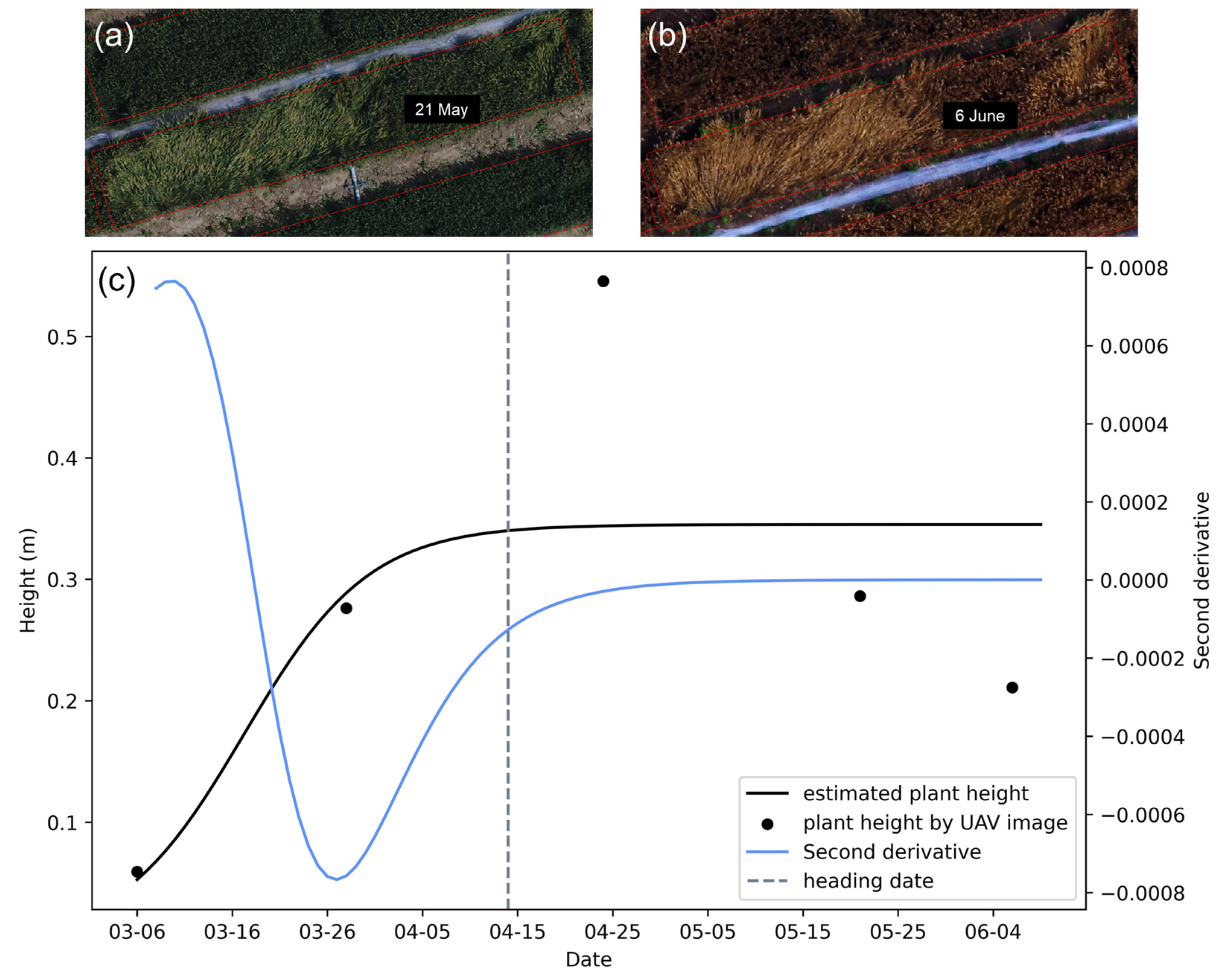
Some plots showed a sharp decrease in plant height at a later growth stage compared to the previous UAV measurements. The plant height in the plot (sowing date: 5 October; variety: Xinong 529; density: 4.5 million plants/ha) decreased markedly on 21 May and 6 June because of lodging, resulting in an abnormal fit of the growth curve (black line) and causing an error in the second derivative (blue line), eventually leading to the largest error (18 d) in the estimated heading date (Figure 7).
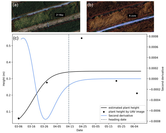
Figure 7.
Abnormal data (lodging) for the plot: sowing date: 5 October; variety: Xinong 529; density: 4.5 million plants/ha. (a) The orthomosaic of 21 May, (b) the orthomosaic of 6 June, and (c) plant height growth curve and second derivative.
3.7. Estimation of Heading Dates before the End of the Growth Period
To test whether the proposed method can estimate wheat heading dates earlier than the end of the growth period, we analyzed 15 plots with sowing date 5 October using the data of the first four-time series (i.e., 6 March, 28 March, 24 April, and 21 May) and the whole region calculation method. Figure 8 shows the growth curves (black lines) for plot (sowing date: 5 October; variety: Jimai 22; density: 4.5 million plants/ha) determined using UAV images of all the time series and the first four-time series, the second derivatives (blue lines), and the heading dates recorded by the experts (the gray dashed lines). We observed heading dates 16 d earlier using the image data for the first four-time series and similar estimation accuracy.
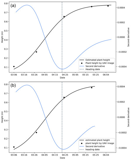
Figure 8.
Growth curves and second derivatives of the plot (sowing date: 5 October; variety: Jimai 22; density: 4.5 million plants/ha). (a) Results obtained from the UAV images of all five-time series, (b) Results obtained from the UAV images of the first four-time series.
The four-time series data for the 15 plots with sowing date 5 October had an MAE of 3.20 d and an RMSE of 3.78 d, which were slightly lower than the estimates obtained from the UAV images of all the five-time series (Table 6). Although the estimation accuracy was lower, the proposed method used less data (the growth curve function had three unknowns, which were solved using four datasets).

Table 6.
Comparison of estimation accuracy of data obtained from the first four- and all five-time series.
4. Discussion
The heading stage is a critical growth period for wheat [36]. Therefore, easy, fast, and high-throughput recordings of wheat heading dates are of great importance for cultivation and breeding research. The proposed UAV image-based method estimated heading dates over 72 plots of three varieties at five sowing dates and five densities. The MAE for the wheat heading date estimation based on the plant height was 2.81 d, which was closer to the dates observed by the experts in the field. Compared to the optimized wheat phenology model (RMSE = 2–7 d) [7] and the adjustment model based on the observations of daily temperatures, vernalization, and photoperiod characteristics for four years (RMSE = 4.24 d; MAE = 3.11 d) [8], our method is simpler and achieves comparable accuracy. Moreover, the MAE of the images taken each day by the field IoTs to estimate the heading date of wheat was 1.34–1.60 d [8]. In addition, in another study, the MAE of the images taken every 5 min by the digital cameras deployed in the field to estimate the heading date of rice was 0.8 d [11]. Although the estimation accuracies of these studies were higher than that of our proposed method, these studies required at least one image [8] or multiple images per day [9,10,11], while only five-time series images were captured and analyzed during the whole wheat growing period (>200 d) in our proposed method (Table 7). Increasing data density (number of observations) in the proposed method is likely to improve the accuracy of heading date estimation. Furthermore, some previous studies estimated the heading dates by detecting wheat or rice ears based on image recognition. However, those studies used empirical thresholds (i.e., number of spikes) to determine the heading dates, with Zhu et al. using the number of spikes in patches as a threshold in an a priori dataset and Bai et al. directly calibrating the threshold at 200, which may vary depending on the variety and the study area [9,10]. Compared to those studies, our proposed method could be used directly in different areas.

Table 7.
The accuracy and the data used compared to previous studies.
In addition, our UAV image-based heading date estimation method has the following two advantages: (1) The method enables simultaneous observations over a large area, whereas the methods proposed in the previous studies have a limited observational range. The proposed method can also be applied with a fixed-wing drone which could capture images for more than 2 h and cover more than 1500 ha [37]. So, if one plot is 10 m2, 1,500,000 plots could be surveyed simultaneously. (2) The method is more cost-effective, which is important in economically underdeveloped areas. The number of experimental plots for genetic breeding and cultivation research is ordinarily very large [13], making the deployment and maintenance of IoTs a considerable capital investment. Moreover, Camera malfunction can also result in erroneous estimates of the crop growth stage [8]. In addition, these methods usually require organ detection and continuous high-frequency and high-resolution acquisition of images, making the images computationally intensive. In the case of fixed camera angle, low spatial resolution, and natural lighting or complex environment, the estimation of heading dates becomes more complicated [9].
In some cases, the proposed method may not work properly. Firstly, some field events (e.g., lodging, Figure 7) will cause underestimating the canopy height, generating the error in crop growth curve fitting and heading dates estimation. Secondly, some field experiment facilities (e.g., sample frame, Figure 3) will cause overestimating the canopy height, influencing the wheat growth curve fitting and heading dates estimation. So, recognizing and removing the abnormal data is helpful for the proposed method. On the other hand, the quantity of the data is also critical. If little data collection is performed for the thousands of experimental plots, the late-developing plots might not be enough to fit a curve because they have fewer valuable data than in the rest of the trial. If n parameters are in the curve fitting function, at least n points are needed [38]. However, just meeting the number of points may not be enough. A common way for an estimate of the parameters is the least-squares method [38,39]. However, it is still challenging to answer whether a least-squares estimate exists [38,40,41]. The distribution of points should be as representative as possible. For example, tightly clustered five points may not be able to estimate the model parameters well. In our study, we used five points to fit the growth curves of 75 plots successfully because of the relatively dispersed time distribution of those points. For sure, more observing points (conducting more UAV flights, although three times is enough for curve fitting, we still recommend five times to avoid fitting failure caused by abnormal data) and making dispersed distribution will help improve the curve fitting and heading dates estimation accuracy for the proposed method.
5. Conclusions
Our study provides a method for estimating high-throughput wheat heading dates based on UAV images with an MAE of 2.81 d, RMSE of 3.49 d. Since our method does not require information about wheat variety, soil, or climate, it has a universal appeal and can directly be used in different areas. In addition, our proposed method is more affordable than the present expert field records and field IoT equipment used to determine heading dates, which is of great significance to promote agricultural research, especially in economically underdeveloped areas. The proposed method can also be applied to other crops or other growth periods associated with changes in plant height. In addition, the different growth periods of crops may be related to other phenotyping parameters such as cover and volume, which can be measured using UAVs and can provide a reference for crop growth monitoring.
There may be some possible limitations in this study. Because the data were collected only five times during the entire wheat growth period and the growth curve function had three unknowns, the temporal resolution of the data was low. We further aim to study and analyze the effects of time density of data acquisition on prediction accuracy and improve the accuracy of heading date estimation.
Supplementary Materials
The following are available online at https://www.mdpi.com/article/10.3390/rs13163067/s1 and https://doi.org/10.5281/zenodo.4777563. Folder S1: growth curve of nine functions, Folder S2: wheat coverage growth curves, Folder S3: wheat plant height growth curves and second derivatives of sampling methods 1, 2, and 3, Folder S4: wheat plant height growth curve by four-time data, Figure S1: value correction of Digital Surface Model, Table S1: Plot designs for field experiments, Table S2: Wheat plant height estimated by full region sampling, Table S3: Wheat plant height estimated by random sampling, Table S4: Wheat plant height estimated of sample 1 by equal interval sampling, Table S5: Wheat plant height estimated of sample 2 by equal interval sampling, Table S6: Wheat plant height estimated of sample 3 by equal interval sampling, Table S7: Wheat plant height estimated of sample 4 by equal interval sampling, Table S8: Wheat plant height estimated of sample 5 by equal interval sampling, Table S9: Heading dates obtained by experts and estimated by sampling methods 1, 2, and 3, Table S10: Estimated heading date of equal interval sampling.
Author Contributions
L.Z. and W.G. conceived the idea and designed the experiments; L.Z. collected UAV images, performed the experiments, analyzed the data, and wrote the manuscript with the input of W.G., C.W., Y.D.; J.W. conducted field experiments; H.W. helped the coding; Y.S. and W.W. supervised this study. All authors have read and agreed to the published version of the manuscript.
Funding
This research was supported by the National Natural Science Foundation of China (U19A2061), the International Science & Technology Innovation Program of the Chinese Academy of Agricultural Sciences (CAASTIP, CAAS-ZDRW202107), and the Japan Science and Technology Agency (JST) CREST program JPMJCR1512, SICORP Program JPMJSC16H2.
Institutional Review Board Statement
Not applicable.
Informed Consent Statement
Not applicable.
Data Availability Statement
Not applicable.
Acknowledgments
We would like to thank the technical staff of the Institute of Cotton Research, Shanxi Agricultural University. We also thank the anonymous reviewers and members of the editorial team for their comments and contributions.
Conflicts of Interest
The authors declare no conflict of interest.
References
- Schmidhuber, J.; Tubiello, F.N. Global food security under climate change. Proc. Natl. Acad. Sci. USA 2007, 104, 19703–19708. [Google Scholar] [CrossRef] [PubMed]
- Tilman, D.; Balzer, C.; Hill, J.; Befort, B.L. Global food demand and the sustainable intensification of agriculture. Proc. Natl. Acad. Sci. USA 2011, 108, 20260–20264. [Google Scholar] [CrossRef]
- Myers, S.S.; Smith, M.R.; Guth, S.; Golden, C.D.; Vaitla, B.; Mueller, N.D.; Dangour, A.D.; Huybers, P. Climate Change and Global Food Systems: Potential Impacts on Food Security and Undernutrition. Annu. Rev. Public. Health 2017, 38, 259–277. [Google Scholar] [CrossRef] [PubMed]
- IFPRI. Actions and Accountability to Advance Nutrition & Sustainable Development—Global Nutrition Report 2015; International Food Policy Research Institute: Washington, DC, USA, 2015; p. 3. [Google Scholar]
- Ihsan, M.Z.; El-Nakhlawy, F.S.; Ismail, S.M.; Fahad, S.; Daur, I. Wheat Phenological Development and Growth Studies As Affected by Drought and Late Season High Temperature Stress under Arid Environment. Front. Plant Sci. 2016, 7, 795. [Google Scholar] [CrossRef]
- Yu, Z.; Cao, Z.; Wu, X.; Bai, X.; Qin, Y.; Zhuo, W.; Xiao, Y.; Zhang, X.; Xue, H. Automatic image-based detection technology for two critical growth stages of maize: Emergence and three-leaf stage. Agric. For. Meteorol. 2013, 174–175, 65–84. [Google Scholar] [CrossRef]
- Kawakita, S.; Takahashi, H.; Moriya, K. Prediction and parameter uncertainty for winter wheat phenology models depend on model and parameterization method differences. Agric. For. Meteorol. 2020, 290. [Google Scholar] [CrossRef]
- Velumani, K.; Madec, S.; de Solan, B.; Lopez-Lozano, R.; Gillet, J.; Labrosse, J.; Jezequel, S.; Comar, A.; Baret, F. An automatic method based on daily in situ images and deep learning to date wheat heading stage. Field Crop. Res. 2020, 252. [Google Scholar] [CrossRef]
- Zhu, Y.; Cao, Z.; Lu, H.; Li, Y.; Xiao, Y. In-field automatic observation of wheat heading stage using computer vision. Biosyst. Eng. 2016, 143, 28–41. [Google Scholar] [CrossRef]
- Bai, X.; Cao, Z.; Zhao, L.; Zhang, J.; Lv, C.; Li, C.; Xie, J. Rice heading stage automatic observation by multi-classifier cascade based rice spike detection method. Agric. For. Meteorol. 2018, 259, 260–270. [Google Scholar] [CrossRef]
- Desai, S.V.; Balasubramanian, V.N.; Fukatsu, T.; Ninomiya, S.; Guo, W. Automatic estimation of heading date of paddy rice using deep learning. Plant Methods 2019, 15, s13007–s13019. [Google Scholar] [CrossRef]
- Wang, X.; Xuan, H.; Evers, B.; Shrestha, S.; Pless, R.; Poland, J. High-throughput phenotyping with deep learning gives insight into the genetic architecture of flowering time in wheat. Gigascience 2019, 8. [Google Scholar] [CrossRef]
- Nishimura, T.; Sasaki, K.; Yamaguchi, T.; Takahashi, H.; Yamagishi, J.; Kato, Y. Detection and characterization of quantitative trait loci for coleoptile elongation under anaerobic conditions in rice. Plant Prod. Sci. 2020, 23, 374–383. [Google Scholar] [CrossRef]
- Holman, F.; Riche, A.; Michalski, A.; Castle, M.; Wooster, M.; Hawkesford, M. High Throughput Field Phenotyping of Wheat Plant Height and Growth Rate in Field Plot Trials Using UAV Based Remote Sensing. Remote Sens. 2016, 8, 1031. [Google Scholar] [CrossRef]
- Guo, W.; Zheng, B.; Duan, T.; Fukatsu, T.; Chapman, S.; Ninomiya, S. EasyPCC: Benchmark Datasets and Tools for High-Throughput Measurement of the Plant Canopy Coverage Ratio under Field Conditions. Sensors 2017, 17, 798. [Google Scholar] [CrossRef]
- Hu, P.; Guo, W.; Chapman, S.C.; Guo, Y.; Zheng, B. Pixel size of aerial imagery constrains the applications of unmanned aerial vehicle in crop breeding. ISPRS J. Photogramm. Remote Sens. 2019, 154, 1–9. [Google Scholar] [CrossRef]
- Smigaj, M.; Gaulton, R.; Suárez, J.C.; Barr, S.L. Canopy temperature from an Unmanned Aerial Vehicle as an indicator of tree stress associated with red band needle blight severity. For. Ecol. Manag. 2019, 433, 699–708. [Google Scholar] [CrossRef]
- Crusiol, L.G.T.; Nanni, M.R.; Furlanetto, R.H.; Sibaldelli, R.N.R.; Cezar, E.; Mertz-Henning, L.M.; Nepomuceno, A.L.; Neumaier, N.; Farias, J.R.B. UAV-based thermal imaging in the assessment of water status of soybean plants. Int. J. Remote Sens. 2020, 41, 3243–3265. [Google Scholar] [CrossRef]
- Turner, D.J.; Malenovsky, Z.; Lucieer, A.; Turnbull, J.D.; Robinson, S.A. Optimizing Spectral and Spatial Resolutions of Unmanned Aerial System Imaging Sensors for Monitoring Antarctic Vegetation. IEEE J. Sel. Top. Appl. Earth Obs. Remote Sens. 2019, 12, 3813–3825. [Google Scholar] [CrossRef]
- Jay, S.; Baret, F.; Dutartre, D.; Malatesta, G.; Héno, S.; Comar, A.; Weiss, M.; Maupas, F. Exploiting the centimeter resolution of UAV multispectral imagery to improve remote-sensing estimates of canopy structure and biochemistry in sugar beet crops. Remote Sens. Environ. 2019, 231. [Google Scholar] [CrossRef]
- Bendig, J.; Bolten, A.; Bennertz, S.; Broscheit, J.; Eichfuss, S.; Bareth, G. Estimating Biomass of Barley Using Crop Surface Models (CSMs) Derived from UAV-Based RGB Imaging. Remote Sens. 2014, 6, 10395–10412. [Google Scholar] [CrossRef]
- Maimaitijiang, M.; Sagan, V.; Sidike, P.; Hartling, S.; Esposito, F.; Fritschi, F.B. Soybean yield prediction from UAV using multimodal data fusion and deep learning. Remote Sens. Environ. 2020, 237. [Google Scholar] [CrossRef]
- Li, B.; Xu, X.; Zhang, L.; Han, J.; Bian, C.; Li, G.; Liu, J.; Jin, L. Above-ground biomass estimation and yield prediction in potato by using UAV-based RGB and hyperspectral imaging. ISPRS J. Photogramm. Remote Sens. 2020, 162, 161–172. [Google Scholar] [CrossRef]
- Siebring, J.; Valente, J.; Domingues Franceschini, M.H.; Kamp, J.; Kooistra, L. Object-Based Image Analysis Applied to Low Altitude Aerial Imagery for Potato Plant Trait Retrieval and Pathogen Detection. Sensors 2019, 19, 5477. [Google Scholar] [CrossRef]
- Jiang, Y.; Li, C.; Paterson, A.H.; Robertson, J.S. DeepSeedling: Deep convolutional network and Kalman filter for plant seedling detection and counting in the field. Plant Methods 2019, 15, 141. [Google Scholar] [CrossRef]
- Borra-Serrano, I.; De Swaef, T.; Quataert, P.; Aper, J.; Saleem, A.; Saeys, W.; Somers, B.; Roldán-Ruiz, I.; Lootens, P. Closing the Phenotyping Gap: High Resolution UAV Time Series for Soybean Growth Analysis Provides Objective Data from Field Trials. Remote Sens. 2020, 12, 1644. [Google Scholar] [CrossRef]
- Chang, A.; Jung, J.; Maeda, M.M.; Landivar, J. Crop height monitoring with digital imagery from Unmanned Aerial System (UAS). Comput. Electron. Agric. 2017, 141, 232–237. [Google Scholar] [CrossRef]
- The People’s Government of Salt Lake District. Y.C. Yuncheng Climate and Environment. Available online: http://www.yanhu.gov.cn/zjyh/yhrw/qhhj/index.shtml (accessed on 17 November 2020).
- Zadoks, J.C.; Chang, T.T.; Konzak, C.F. A decimal code for the growth stages of cereals. Weed Res. 1974, 14, 415–421. [Google Scholar] [CrossRef]
- Wang, H.; Duan, Y.; Shi, Y.; Kato, Y.; Ninomiya, S.; Guo, W. EasyIDP: A Python Package for Intermediate Data Processing in UAV-Based Plant Phenotyping. Remote Sens. 2021, 13, 2622. [Google Scholar] [CrossRef]
- Verhulst, P.F. Recherches Mathématiques sur la loi D’accroissement de la Population, par P.F. Verhulst; M. Hayez: Brussels, Belgium, 1845. [Google Scholar]
- Harahagazwe, D.; Condori, B.; Barreda, C.; Bararyenya, A.; Byarugaba, A.A.; Kude, D.A.; Lung’aho, C.; Martinho, C.; Mbiri, D.; Nasona, B.; et al. How big is the potato (Solanum tuberosum L.) yield gap in Sub-Saharan Africa and why? A participatory approach. Open Agric. 2018, 3, 180–189. [Google Scholar] [CrossRef]
- Luo, S.; He, Y.; Li, Q.; Jiao, W.; Zhu, Y.; Zhao, X. Nondestructive estimation of potato yield using relative variables derived from multi-period LAI and hyperspectral data based on weighted growth stage. Plant Methods 2020, 16, 150. [Google Scholar] [CrossRef]
- Shi, P.-J.; Chen, L.; Hui, C.; Grissino-Mayer, H.D. Capture the time when plants reach their maximum body size by using the beta sigmoid growth equation. Ecol. Model. 2016, 320, 177–181. [Google Scholar] [CrossRef]
- Virtanen, P.; Gommers, R.; Oliphant, T.E.; Haberland, M.; Reddy, T.; Cournapeau, D.; Burovski, E.; Peterson, P.; Weckesser, W.; Bright, J.; et al. SciPy 1.0: Fundamental algorithms for scientific computing in Python. Nat. Methods 2020, 17, 261–272. [Google Scholar] [CrossRef]
- Grogan, S.M.; Anderson, J.; Baenziger, P.S.; Frels, K.; Guttieri, M.J.; Haley, S.D.; Kim, K.-S.; Liu, S.; McMaster, G.S.; Newell, M.; et al. Phenotypic Plasticity of Winter Wheat Heading Date and Grain Yield across the US Great Plains. Crop Sci. 2016, 56, 2223–2236. [Google Scholar] [CrossRef]
- Zhao, L.; Shi, Y.; Liu, B.; Hovis, C.; Duan, Y.; Shi, Z. Finer Classification of Crops by Fusing UAV Images and Sentinel-2A Data. Remote Sens. 2019, 11, 3012. [Google Scholar] [CrossRef]
- Jukić, D.; Kralik, G.; Scitovski, R. Least-squares fitting Gompertz curve. J. Comput. Appl. Math. 2004, 169, 359–375. [Google Scholar] [CrossRef][Green Version]
- Björck, A. Numerical Methods for Least Squares Problems; Society for Industrial and Applied Mathematics: Philadelphia, PA, USA, 1996; p. 424. [Google Scholar] [CrossRef]
- Demidenko, E. On the existence of the least squares estimate in nonlinear growth curve models of exponential type. Commun. Stat. Theory Methods 1996, 25, 159–182. [Google Scholar] [CrossRef]
- Demidenko, E. Is this the least squares estimate? Biometrika 2000, 87, 437–452. [Google Scholar] [CrossRef]
Publisher’s Note: MDPI stays neutral with regard to jurisdictional claims in published maps and institutional affiliations. |
© 2021 by the authors. Licensee MDPI, Basel, Switzerland. This article is an open access article distributed under the terms and conditions of the Creative Commons Attribution (CC BY) license (https://creativecommons.org/licenses/by/4.0/).

