Abstract
Urban forests are an important part of any city, given that they provide several environmental benefits, such as improving urban drainage, climate regulation, public health, biodiversity, and others. However, tree detection in cities is challenging, given the irregular shape, size, occlusion, and complexity of urban areas. With the advance of environmental technologies, deep learning segmentation mapping methods can map urban forests accurately. We applied a region-based CNN object instance segmentation algorithm for the semantic segmentation of tree canopies in urban environments based on aerial RGB imagery. To the best of our knowledge, no study investigated the performance of deep learning-based methods for segmentation tasks inside the Cerrado biome, specifically for urban tree segmentation. Five state-of-the-art architectures were evaluated, namely: Fully Convolutional Network; U-Net; SegNet; Dynamic Dilated Convolution Network and DeepLabV3+. The experimental analysis showed the effectiveness of these methods reporting results such as pixel accuracy of 96,35%, an average accuracy of 91.25%, F1-score of 91.40%, Kappa of 82.80% and IoU of 73.89%. We also determined the inference time needed per area, and the deep learning methods investigated after the training proved to be suitable to solve this task, providing fast and effective solutions with inference time varying from 0.042 to 0.153 minutes per hectare. We conclude that the semantic segmentation of trees inside urban environments is highly achievable with deep neural networks. This information could be of high importance to decision-making and may contribute to the management of urban systems. It should be also important to mention that the dataset used in this work is available on our website.
1. Introduction
Urbanization displays a massively increasing global trend. According to data of the UN [1], more than half of the world’s population habit urban areas, and by 2050, it is projected to 68% of the world’s population to be urban. The cities can be interpreted as a complex system that incorporates people and diffusion and exchange of work, assets, capital, and information. One of the essential aspects of a city is the vegetation; they provide the residents of the city with several environmental and social services, in this way supporting the development and improving inhabitants quality of life [2,3,4,5,6]. The types of services that the urban forests provide can be cited as regulating and maintaining local climatic conditions by reducing the formation of urban heat islands, provide habitat for local biodiversity, provisioning resources (e.g., wood, food, and biomass), cultural and historical values and also scenic landscapes [7,8,9,10,11]. According to [12], urban forests can be categorized in three primary forms, such as (i) forest remnants occurring either in the urban perimeter or in the urban-rural interface and contains a large number of trees, (ii) green areas over a given landscape that presented different tree species devoted to meet social, aesthetic and architectural benefits, ecological needs and even economic benefits and (iii) street trees that are any trees along public roads, whether on sidewalks or in flowerbeds. Urban growth is usually associated with forest remnants suppression leading to ecosystem stress and biodiversity losses [13]. In the urban environment, vegetation suppression is mainly correlated to the urban process of growth and often results in impervious areas and brings other negative impacts for the environment, such as urban biodiversity loss and changes in the hydrodynamics of the cities [14]. Therefore, mapping urban forests are essential in order to propose strategies that optimize citizen’s quality of life, city hydrodynamics, and biodiversity by preserving and improving this valuable ecosystem [2,15].
The capability of detecting individuals and groups of trees is essential for many applications in forest monitoring according to [16], such as resource inventories, wildlife habitat mapping; biodiversity assessment; and threat and stress management. Nevertheless, the task of mapping trees, especially for an urban context, is a crucial procedure for environmental planning [10,17]. The urban tree segmentation task refers to the automated classification of each pixel of a given image into a tree or background, and that is a challenging problem. As highlighted before, urban forests are a particular form of forest with unusual characteristics as they can be isolated, densely, or sparsely distributed and mixed with other urban features [18]. All these characteristics make automated urban forest mapping a complex computational task. Therefore, it requires high spatial resolution images and a robust machine learning process to differentiate them as objects. The consolidated approach for mapping trees using remote sensing refers to the use of data acquired from sensors embedded in satellite, airplane, or Unmanned Aerial Vehicles (UAV) [19,20,21,22,23,24]. Remote sensing can provide valuable data at different acquisition levels to support policies related to urban forest mappings such as forest health, regulation, climate change mitigation, and long-term sustainability. As a result, continuous remote sensing tracking of forest patterns allows for cost-effective periodical assessment of vegetated areas [25], supporting decision making.
Artificial intelligence and the remote sensing field are allies of an extended period. As a subgroup of the machine learning area, deep neural networks improved performance for extracting information from images. Deep learning-based methods are evolving continuously, and their high performances being confirmed in several fields of applications [26,27,28,29,30,31,32,33]. As an example of advances in this field of study, we will briefly describe some works. Ref. [34] proposed a methodological approach for detecting individual fruits using a pixel-wise segmentation method based on Mask R-CNN and multi-modal deep learning models. It used RGB and HSV images, and the results revealed a more precision score when deep learning models are trained with RGB and HSV datasets altogether. Ref. [35] opens opportunities for a better understanding of the on-ground feature mapping by using simplified deep learning methods. By adopting high spatial resolution remote sensing data and models of dynamic multi-context segmentation approach, based on convolutional networks, Ref. [35] research showed improvements in pixel-wise classification accuracy when compared to state-of-the-art deep learning methods. One research [30] evaluated five methods based on deep fully convolutional networks using high-spatial-resolution RGB images to map a specific threatened tree species finding out an overall accuracy ranging from 88.9% to 96.7%. The research of Zamboni et al. [36] propose the evaluation of novel methods for single tree crown detection. A total of 21 methods were investigated, including anchor-based (one and two-stage) and anchor-free state-of-the-art deep-learning methods. Here, the authors focused on generating bounding boxes in each tree, not in the tree segmentation.
The accurate segmentation of urban forests is a relevant matter, as it aims to support management decisions related to urban environmental planning. So this work intends to provide a low-cost and effective method of mapping trees inside the urban areas. Our study area is a metropolitan region from Brazil, inserted in Cerrado Biome called Campo Grande. The trees of the metropolitan region are very diverse, having as many as 61 cataloged tree species that are common encountered in the city center and avenues [37]. Cerrado is a nature hotspot that is rich in biodiversity, has endemic species (species of plants or animals that only occur in that Biome), and whose maintenance is threatened. Therefore, they are places that need more attention from conservation programs. The Cerrado, together with the Atlantic Forest, are the two areas considered as hotspots in Brazil. The expansion of agriculture, especially in the Brazilian Cerrado, which has an ideal climate for cultivating various crops, generated pressure to suppress natural areas of this Biome, increasingly threatening its existence. The monitoring through technology allows for more effective planning of actions and acts quickly to curb vegetation removal without permission.
Therefore, our originality comes from the dataset and the exertion of deep learning algorithms to improve the nature conservation efforts in this region, and our primary contribution is related to the investigation of state-of-the-art semantic segmentation methods to detect trees in urban areas. For this task, we used data with a high spatial resolution (Ground Sample Distance (GSD) of 10 cm) inside an urban area inside the Cerrado biome and used five state-of-the-art deep learning architectures to process the data. Deep learning-based approaches designed to tackle this task receive, as input, an image and return as output, another image, generally with the exact size of the input data with each pixel associated with one class. We choose to use deep learning because they present a better performance in semantic segmentation and scene interpretation tasks over traditional machine learning and trained professionals in many fields of science as demonstrated by [38,39,40,41,42].
The rest of this paper is organized as follows: Section 2 provides detailed info of the urban area and methods applied; Section 3 explored the results; Section 4 argues the implications of the results of the methods applied in this research and in Section 5 we conclude the paper and provides some futures directions for this and other studies.
2. Materials and Methods
Our workflow was divided into five main stages (Figure 1). In (a) we have the RGB-imagery acquisition by an Airplane flight performed in the metropolitan region of Campo Grande, State of Mato Grosso do Sul, Brazil, in the heart of the Cerrado Biome. (b) presents a geometric correction of the images and orthophotos generation. In (c), annotation of the trees in the orthophotos, and preparation of the data by splitting it into test and training subsets. In (d), evaluation of five state-of-the-art deep neural networks selected for the proposed task. Finally, in (e), comparison of the performance of the methods.
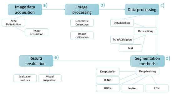
Figure 1.
Workflow summarizing the fundamental steps of the conducted approach. Adapted from [43].
2.1. Data Acquisition and Image Processing
The imagery-dataset was acquired with an airplane flight performed in Campo Grande, Mato Grosso do Sul. This flight took place in 2013 and created a total of 1394 RGB orthoimages with 5619 × 5946 pixels each, with dimensions of 561.9 × 594.6 m and a ground sampling distance of 10 cm. It is important to note that the images are not overlapped. Inside our study area, the urban forests are randomly distributed and mixed between the constructions (Figure 2). Inside the study area, there are a substantial diversity of tree species, many of them are not natives trees, as the region is a neighborhood area where citizens tend to plant the trees following some local set of rules as of the size of the tree, but besides that, they tend to plant trees that pleases then the most.
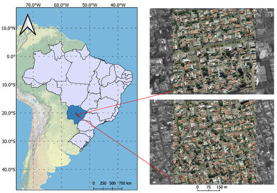
Figure 2.
Overall visualization of the study area, the location is inside the metropolitan region of Campo Grande, Mato Grosso do Sul, Brazil. And also in color a visualization of the two base images used to make the labels of the tree canopies.
For the classification quality assessment of the deep learning algorithms, we select two images from this dataset and manually labeled all the trees presented in them, mapping all the tree cover in these two images. The images have 33.4 hectares (ha) each and a tree cover of 4.8 ha in one image and 3.8 ha in the other. All tress are randomly distributed in the area, making a ratio of 12.8% of the dataset composed of our target object and the rest being background, that is composed of roads, buildings, cars, houses, and many other elements that compose a typical urban environment, e.g., paths, districts, edges, nodes, and landmarks).
2.2. Semantic Segmentation Methods and Experimental Setup
This section presents five state-of-the-art deep learning architectures evaluated in our study case. These architecture were the same applied in the work of [43], our previous work with precision agriculture, but now we want to attend the urban forest context. To better visualize and analyze CNN’s architectures, we organize the CNN structure illustrations with colored blocks. Each block represents a processing layer with the data as described in Figure 3.

Figure 3.
Building blocks used to illustrate the different CNNs layers.
Fully Convolutional Network (FCN): FCN architecture is presented in Figure 4. It was proposed by [44]. This deep network creates a classification map with a set of convolutional layers returning a spatially reduced result. After that, it applies deconvolution layers to upsample the initial classification and produce a dense prediction, restoring the image’s original resolution.
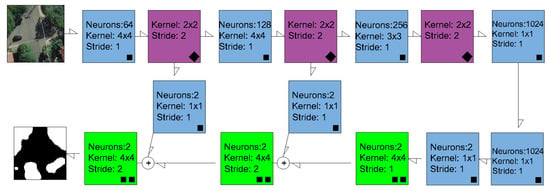
Figure 4.
Fully Convolutional Network (FCN) architecture. Adapted from [43,44].
U-Net and SegNet: According to [43], the U-Net architecture was the first network to propose an encoder-decoder architecture to perform semantic segmentation tasks. This deep network was created by [45] to segment biomedical images. To generate an initial prediction map, are used the encoder and max-pooling layers with feature extraction. The encoder consists of a stack of convolution, and the decoder comprises convolutions, deconvolutions, and unpooling layers in a symmetrical expanding path, using deconvolution filters to up-sample the feature maps. An illustration of this architecture is presented in (Figure 5). SegNet is also an encoder-decoder network path like U-Net, but with the replacement of the deconvolution layers by unpooling operations to increase the spatial resolution of the initial prediction map generated by the encoder. Ref. [46] proposed this architecture based on the VVG 16 network developed by [47]. A scheme of deep network SegNet is shown in (Figure 6).
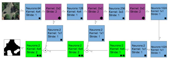
Figure 5.
U-Net architecture. Adapted from [43,45].

Figure 6.
SegNet architecture. Adapted from [43,46].
DeepLabV3+: The DeepLabV3+ [48] starts with three blocks composed of two convolutions and one polling layer that performs the feature extraction and an initial prediction map. These features are then processed by a particular layer, called Atrous Spatial Pyramid Pooling (ASPP) introduced in [49]. This technique involves employing atrous convolution in parallel to extract features at multiple scales and alleviate the loss of spatial information due to prior pooling or convolutions with striding operations. The data is then processed with features extracted from the first pooling layer and refined by one extra convolutional layer. Then three convolutional layers process the concatenated segments upsampled by a bilinear interpolation producing the final prediction map. For more details, see Figure 7 [48].

Figure 7.
DeepLabV3+ architecture. Adapted from [43,48].
Dynamic Dilated Convolutional Network (DDCN): Proposed by [35], the DDCN is designed to preserve the input image resolution. Ref. [43] describe this network in more detail. However, in summary, the Dynamic Dilated Convolutional Network uses a multi-scale training strategy that implements dynamically-generated input images to converge a dilated model that does not downsample the input data due to a specific configuration of stride and padding. The model has eight dilated blocks; each block comprises a dilated convolution and a pooling layer; the blocks are followed by a standard convolutional layer responsible for the final prediction map. In each iteration of the training procedure, a dimension is randomly selected from this distribution and used to create a new batch. The model captures multi-scale information by processing these batches with a pre-determined size, advancing in the processing phase. The network selects, based on scores obtained during the training phase for each evaluated input size, the best image resolution. Then the DDCN processes the testing images using batches composed of the images with the best-evaluated size (Figure 8).
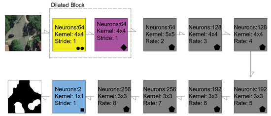
Figure 8.
Dynamic Dilated Convolutional Network (DDCN) architecture. Adapted from [35,43].
2.2.1. Experimental details
We adopted the same training/trial protocol for all CNNs. All networks used in this research have been trained from scratch (i.e., without pre-trained weights from other datasets, like ImageNet, for example). We used 1938 input patch sizes of 256 × 256 pixels, with 388 patches for the test, 1162 for train, and 388 for validation, a distribution of approximately 20%, 60%, and 20% respectively. It is important to note that additional input patch sizes were tested in an experimental phase, but the results did not change considerably and only increased the training time. All approaches used the same set of hyperparameters during training, which was defined based on previous analyses. Specifically, the learning rate, weight decay, momentum, and iterations were 0.01, 0.005, 0.9, and 200,000, respectively. The model is optimized using stochastic gradient descent (SGD). To assist the convergence process and prevent overfitting (Overfitting is a concept used to refer to a model that adjusts too well to the training data, but it does not generalize to the unseen before dataset, i.e., a test dataset), after 50,000 iterations, the learning rate was reduced following an exponential decay parameter of 0.5 by an SGD scheduler. Aside from this, we used rotation, noise, and flip (as in [50]) for data augmentation, and we were capable of augmenting the dataset by six times. With the data augmentation technique, we can make the CNN classification more robust and generalize better. In Figure 9, we can see the schematic diagram for the evaluation process.
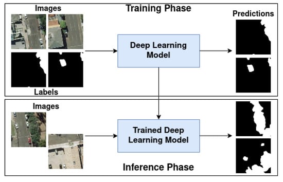
Figure 9.
Schematic diagram of the evaluation process.
All deep learning-based models exploited in this work were implemented using the TensorFlow [51], a Python framework conceived to allow efficient analysis and implementation of deep learning with Graphics Processing Units (GPUs). All experiments conducted here were performed on a 64-bit Intel i7-8700K@3.70GHz CPU workstation, 64 GB memory, and NVIDIA® GTX 1080 GPU with 12Gb of memory, under a 10.0 CUDA version. Debian 4.195.98-1 version was used as the operating system.
2.2.2. Evaluation Metrics
The networks were evaluated using five different classification metrics: pixel accuracy, average Accuracy, F1-score, Kappa, IoU/Jaccard. The variables TP, TN, FP, FN stand for the number of true positives, true negatives, false positives and false negatives, respectively. In our analysis, and refer to the pixels assigned by the underlying classifier to the trees and background classes, respectively. Such and are or , depends on whether or not they agree with the ground truth, respectively.
The Pixel accuracy is given by:
The average accuracy (Av. Acc.) is the mean accuracy result given by class, in this case we have 2 classes tree and background.
The F1-score is given by:
where P and R stand for Precision and Recall, respectively, and are given by the ratios present in Equations (3) and (4):
The Cohen’s Kappa statistic (K) proposed by [52], tells you how much better your classifier is performing over the performance of a classifier that guesses at random according to the frequency of each class. The mathematical formulation of this metric is given by a balance between a positive and negative response, as follows:
The Union Intersect (IoU), also known as the Jaccard Index, is frequently used as a precision metric for semantic segmentation tasks [53,54]. In the Reference and the Prediction mask, IoU is indicated by a ratio of the number of pixels in both masks to the total number of pixels in:
3. Results
In this section, we present the results of the experimental evaluation of the selected semantic segmentation approaches. In (Section 3.1) we made a quantitative analysis with the metrics described in (Section 2.2.2), the (Section 3.3) presents a visual analysis of the segmentation outcomes, and in (Section 3.2), we assess the computational efficiency of each method.
3.1. Performance Evaluation
The evaluated deep learning methods returned similar results for the proposed approach. Ranging from 96.18% to 95.56% for pixel accuracy, 91.25% to 88.80% for Av. Acc., 91.40% to 89.91% for F1-score, 82.20% to 79.83% for Kappa and 73.89% to 70.01% for IoU. Results of the classification for the test set are presented in Table 1.

Table 1.
Classifiers’ results for each evaluation metrics using the test set of patches, while classifying tree canopies.
A slight difference indicates that DeepLabV3+ was the best classifier method from a quantitative perspective, returning the best available results for the chosen metrics. In the recent few years, the architecture DeepLabv3+ has been regarded as state-of-the-art in semantic segmentation. So it is no surprise that it achieved the best performance among all tested architectures in our experiments, both in terms of absolute average accuracies as in terms of variability for the test set. Nevertheless, it also is accurate to say by analyzing the results presented in Table 1 that all of the five state-of-the-art networks are capable of segmenting trees inside a Cerrado urban environment in a satisfactory way with the proposed imagery dataset. These deep neural networks can separate tree covered-area from other objects inside an urban environment while maintaining the original resolution of the image input is an important characteristic, making it possible to extract valuable information that could be used to support urban planning strategies.
Figure 10 presents the confusion matrix of all the CNN methods used in this research, which was used to derive the metrics presented in Table 1.
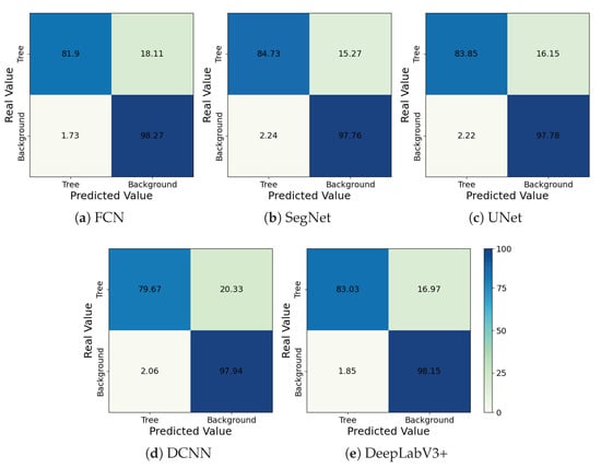
Figure 10.
Confusion Matrix for all the analysed ConvNets.
Finally, we present in Figure 11 the accuracy and loss curves. We can see that the FCN, UNet, and SegNet performed similarly with stable slight variation and close to the minimum loss value after 100,000 iterations or half the way of the learning process established. The DCNN presented some increase in loss after 100,000 iterations. After the learning rate was reduced in the lasts 50,000 iterations by the SGD scheduler, it reached its minimum value, and the loss fluctuations were reduced. Moreover, the DeepLabV3+ became stable after 100,000 iterations with the minimum loss observed.
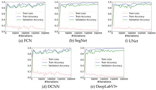
Figure 11.
Convergence of the evaluated networks.
3.2. Computational Complexity
This section compares the methods in terms of computational efficiency and computational load for training and inference. Table 2 presents the average training and inference times measured on the hardware infrastructure described in Section 2.2. Considering that the methods were trained with the same optimizer and learning rates, these results are highly correlated with the network depth and the selected batch size. For instance, the DDCN network is deeper than the others, and the consequence is that it took longer than the other networks for training and inference.

Table 2.
Number of Parameters and Processing Time of the proposed approaches. The training time represents the results for the test set of each method. The inference time stands for the time taken by each model to make predictions for each image.
The most significant variation of performance is concerning the number of parameters and with training and inference time. Despite being the best architecture in performance, According to Table 2, DeepLabv3+ needed more parameters than the other architectures, about 2.75 times more parameters than the U-Net, the least requiring one. The need for a more significant number of parameters often implies a higher demand for training samples that our dataset or another dataset may not have met that the methods present in this research paper may be applied, possibly causing the DeepLabV3+ architecture to perform below its potential.
3.3. Visual Analysis
Some features maps, learned by the convolutional layers, are presented in Figure 12. Specifically, this image presents low-, mid- and high-level feature maps learned by the first, a middle, and the last layers of the networks, respectively. We can see the each CNN performs very differently from one another.
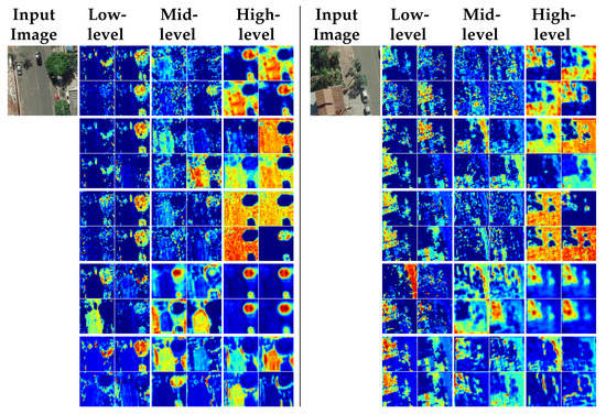
Figure 12.
Input images and some produced (upsampled) feature maps extracted from initial, mid, and end layers of the networks. From top to bottom: FCN [44], UNet [45], Segnet [46], DeepLabV3+ [48], and DCNN [35]. The high level column presents an approximation of the final result of CNN classification.
Figure 13 and Figure 14 show an example of the results for the chosen methods with cropped images from our dataset that came to represent common occurrences of vegetation inside an urban environment. References are presented on the left row of the cropped images in the first line of both Figures, the annotated label is in the second line, and each subsequent line presents the segmentation produced by the CNN. We chose these images to represent the visual segmentation of the dataset because they are different in their content and represent common situations that CNNs may encounter while segmenting a tree in urban areas.
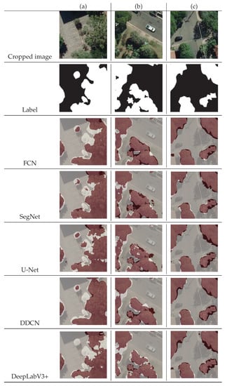
Figure 13.
Cropped images, labeled canopies and the resulting map for the cropped image with the evaluated CNNs. The light red areas are the true positives (TP), the soft grey areas are the true negatives (TN), the white spots are the false negatives (FN), and the dark red areas are the false positives (FP).
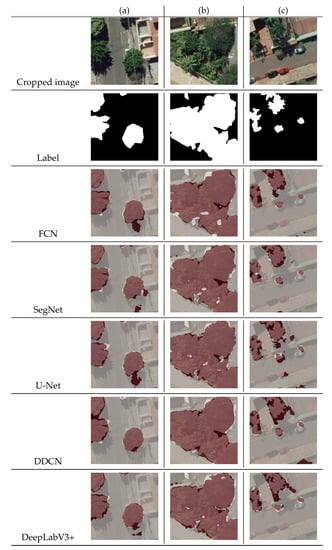
Figure 14.
Cropped images, labeled canopies and the resulting map for the cropped image with the evaluated CNNs. The light red areas are the true positives (TP), the soft grey areas are the true negatives (TN), the white spots are the false negatives (FN), and the dark red areas are the false positives (FP).
In row (a) of Figure 13, there is a parking lot background. Inside this parking lot, we have one large group of trees with sparse distribution, one singular tree in the parking lot, one tree truncated in half by the picture frame, and a shadowed area at the top of the image. The white spots, or false negatives, compose a large area of the photograph, meaning that the CNNs missed a lot of our intended objective, classifying as background much of the trees in this area. However, it is essential to note that shadows were not a problem for any CNNs in this particular case. Another issue was related to the shape of the object. The SegNet, for example, returned a worse response related to it. All the CNNs localized the truncated tree. The errors mainly occurred at the canopies’ edges, meaning that the CNNs missed information regarding vegetation borders. In row (b) of Figure 13, the image possesses a greater variety of backgrounds; a patch of grass, a patch of sidewalk, a patch of road, a car, and a patch of house, and more shadows. Furthermore, there are two large groups of trees with tension lines crossing them in this image, and even a single tree near one of the groups and a small one crop at the top of the image. This region, in particular, highlighted some of the flaws in the segmentation results. The DeepLabV3+ and the DDCN returned higher FN, especially in the shadowed areas. Still, most of the FN cases of this patch are inside the tree group at the bottom, meaning that the CNNs had a hard time separating singular trees in this context. In row (c) of Figure 13, there is a variety of backgrounds as diverse as in row (b), but a uniform distribution of trees inside the image, with four medium size and contiguous groups of canopies. Here, the CNN’s presented fewer mistakes than on the other examples, as most of the errors were FP in the edges of large groups of trees; with this example, we see that the CNNs perform better in patches with groups of trees no isolated trees nearby.
In row (a) of Figure 14, we have large tree canopies and a road with a rooftop background, and all the CNNs performed reasonably well with large canopies segmentation except for U-Net and the FCN that faced a difficult time segmenting the shadowed areas in this case. In row (b) of Figure 14, we have a large patch of trees that are beneath a residential area, and the networks performed similarly in this case of one large group of trees even for the false positives case of the shadows, but we can see that in this case, DeepLabV3+ was the most assertive CNN. In row (c) of Figure 14, we have a small patch of trees located beneath houses and cars. As discussed previously, we have the most significant part of the errors with the isolated and small trees, shadowed areas, and grassed and bush areas.
4. Discussion
A set of state-of-the-art deep learning semantic segmentation approaches was applied to map urban forests in high-resolution RGB imagery in the urban context. Our results indicated that the investigated methods performed fairly similarly in this task, returning a pixel accuracy between 96.18% (DeepLabV3+) and 95.56% (DDCN), an average accuracy between 96.07% (DeepLabV3+) and 95.56% (DDCN), a F1-score between 91.40% (DeepLabV3+) and 89.91% (DDCN), a Kappa 82.80% (DeepLabV3+) and 79.83% (DDCN) and IoU between 73.89% (DeepLabV3+) and 70.01% (DDCN). Visually evaluating the classification map obtained with each network, it is difficult to emphasize an overall better method. Nonetheless, we have a quantitative advantage for the DeepLabV3+. This CNN also presented a satisfactory visual result with little noise and false-positives rates regardless of tree detection. Despite the quantitative results, the DDCN also presented a smooth visual result.
Most of the evaluated methods returned proximal inference time for both GPU and CPU tests, except for the DDCN method [35], which took around four times the amount of time needed to perform the same task. U-Net consistently presented lower inference times, being the fastest method among all for training and prediction. However, an estimation of this inference time per area demonstrates how rapidly these neural networks can segment trees in the given data set once they are trained. This information is vital for precision image segmentation tasks since this response could be incorporated into decision-making strategies regarding area size and priority. It should also be noted that the times informed here are considering the system used to train these methods, see Section 2.2.1.
For a practical approach, the final use of this method is the application in a city to detect vegetated areas. For our example images, we have a range of pixel accuracy of 96.18% to 95.56%. These remaining percentage not correctly classified in our test dataset is explained in Section 3.3 as the CNNs are known for producing errors in image-boundaries [55,56]. Moreover, most of the problems faced by the investigated deep networks are related to shadowy areas, isolated and small trees, and the grass and bush areas inside the images. Things for the CNN and even for the human operator can be a little ambiguous. Some solutions for these kinds of problems are the labeled dataset be manually segmented by more than one operator, creating a more detailed and overlapped map of the trees inside an area, we also can augment the dataset using techniques, such as the presented in the Section 2.2.1. The analysis of the classification results shown in Table 1 demonstrates that the deep neural networks are lacking accuracy if compared to our annotations; the result of the IoU metric demonstrates this. Regardless, the visual output of the segmentation methods is rather noisy in some of the patches. Shadows were a problem, even more, when mixed inside large groups of trees; when they are further away from our object of interest, CNNs have fewer issues in segmenting them. However, small isolated trees were a higher challenge for all the networks to deal with, especially when they are inside the same patch as large groups of trees; all the CNNs tend to miss-classify and even ignore them. The grass and bush areas were more of a problem when they were near large groups of trees, and the CNNs might interpret them as a continuation of the tree patches and classify them as trees, creating false positives.
Possible solutions to contour this problem are to use a higher resolution RGB imagery dataset and use different kinds of datasets in conjunction. For example, we can use RGB and LiDAR fusion to create an exact 3D point cloud; these approaches are a hot topic in autonomous driving vehicles [57,58], for the reason that they have an excellent capacity for accurate and fast scenery reconstruction. Another approach is the use of image segmentation methods with multi-spectral, and high spatial resolution sensors, the exploration of the spectral index for the detection and analysis of vegetation is a mature topic in remote sensing [17,22,59] and it can also be implemented with Deep learning approaches inside urban areas for semantic segmentation tasks.
5. Conclusions
We evaluated five state-of-the-art Convolutional Neural Networks for the semantic segmentation of urban forests using airborne high spatial-resolution RGB images. The architectures tested were: Fully Convolutional Network, U-Net, SegNet, Dynamic Dilated Convolution Network, and DeepLabV3+. The experimental analysis showed the effectiveness of the methods reporting a very proximal value for all the classifiers, with a mean for Pixel accuracy of 96.11% average pixel accuracy of 90.70%, F1-score of 91.27%, Kappa of 82.54% and IoU of 73.56%. With the best results being from the DeepLabV+3 architecture. Our research confirmed that CNNs could segment urban trees from high spatial resolution remote sensing imagery in the urban context. However, the networks still possess some limitations in the urban environment.
For future directions and development, we intend to improve the develop methods to improve the IoU mainly because it was our worst-performing metric. For this, we suggest creating a supplementary labeling phase created by a different human operator of the same area and merging the labels. As we have more correct labels, human error cases will be minimized in the labeling phase, proving a better feature map for the CNNs to work. The labeling phase of a large and complex image is a classical case of estimation error, and to overpass it, another stage of the labeling process is then suggested as an alternative.
We further intend to test the generalization and the transferability of the CNN architectures on datasets from different regions, as the urban landscape are diverse in composition applying the concept of domain adaptation. Future studies should also involve differentiate tree species, and to perform data fusion with multiple sensors data, such as Li-DAR or multi-spectral data in addition to the optical RGB data.We also suggest exploring instance segmentation (detection and segmentation) architectures such as Mask RCNN, Detectron2, FCIS, BlendMask, and YOLACT. These approaches are also of interest to urban planning applications, because they can differentiate the urban landscape by object, contributing to the tree classification by species.
Author Contributions
Methodology, W.N.G., J.M.J., P.T.S.d.O., L.P.O. and J.A.C.M.; software, J.A.d.S. and K.N.; validation, W.N.G., J.M.J., J.A.d.S., K.N., A.P.M.R. and V.L.; formal analysis, V.L., K.N. and J.M.J.; investigation, L.P.O. and J.A.C.M.; resources, V.L. and J.M.J.; data curation, W.N.G., J.M.J. and J.A.C.M.; writing—original draft preparation, J.A.C.M. and L.P.O.; writing—review and editing, V.L., A.P.M.R., F.D.G.G., D.A.S., D.E.G.F., K.N. and J.M.J.; visualization, J.A.C.M. and K.N.; supervision, W.N.G., V.L. and J.M.J.; project administration, W.N.G. and J.M.J.; funding acquisition, J.M.J., V.L. and W.N.G. All authors have read and agreed to the published version of the manuscript.
Funding
This research was funded by the Brazilian National Council for Scientific and Technological Development (CNPq) p: (310517/2020-6, 303559/2019-5, 313887/2018-7, 433783/2018-4 and 304173/2016-9), the Coordination for the Improvement of Higher Education Personnel (CAPES) Print p: (88881.211850/2018-01), and the Foundation to Support the Development of Education, Science and Technology of the State of Mato Grosso do Sul (FUNDECT) p: (59/300.066/2015 and 59/300.095/2015).
Data Availability Statement
The data presented in this study are openly available, access through link: https://sites.google.com/view/geomatics-and-computer-vision/home/datasets (accessed on 16 July 2021).
Acknowledgments
We would like to thank the Graduate Program of Environmental Technologies of the Federal University of Mato Grosso do Sul (UFMS) to support the doctoral dissertation of the first author and the Coordination for the Improvement of Higher Education Personnel (CAPES). We also would like to thank the editors and three reviewers for providing constructive concerns and suggestions. Such feedback helped us improve the quality of the manuscript.
Conflicts of Interest
The authors declare no conflict of interest.
References
- World Urbanization Prospects—Population Division—United Nations. 2018. Available online: https://population.un.org/wup/Publications/Files/WUP2018-Highlights.pdf (accessed on 16 July 2021).
- La Rosa, D.; Wiesmann, D. Land cover and impervious surface extraction using parametric and non-parametric algorithms from the open-source software R: An application to sustainable urban planning in Sicily. GIScience Remote Sens. 2013. [Google Scholar] [CrossRef]
- Jennings, V.L.L.; Yun, J. Advancing Sustainability through Urban Green Space: Cultural Ecosystem Services, Equity, and Social Determinants of Health. Int. J. Environ. Res. Public Health 2016, 13, 196. [Google Scholar] [CrossRef] [PubMed] [Green Version]
- Arantes, B.L.; Castro, N.R.; Gilio, L.; Polizel, J.L.; da Silva Filho, D.F. Urban forest and per capita income in the mega-city of Sao Paulo, Brazil: A spatial pattern analysis. Cities 2021, 111, 103099. [Google Scholar] [CrossRef]
- Jim, C.; Chen, W.Y. Ecosystem services and valuation of urban forests in China. Cities 2009, 26, 187–194. [Google Scholar] [CrossRef]
- Chen, W.Y.; Wang, D.T. Urban forest development in China: Natural endowment or socioeconomic product. Cities 2013, 35, 62–68. [Google Scholar] [CrossRef]
- Baró, F.; Chaparro, L.; Gómez-Baggethun, E.; Langemeyer, J.; Nowak, D.J.; Terradas, J. Contribution of ecosystem services to air quality and climate change mitigation policies: The case of urban forests in Barcelona, Spain. Ambio 2014. [Google Scholar] [CrossRef] [Green Version]
- McHugh, N.; Edmondson, J.L.; Gaston, K.J.; Leake, J.R.; O’Sullivan, O.S. Modelling short-rotation coppice and tree planting for urban carbon management—A citywide analysis. J. Appl. Ecol. 2015. [Google Scholar] [CrossRef]
- Kardan, O.; Gozdyra, P.; Misic, B.; Moola, F.; Palmer, L.J.; Paus, T.; Berman, M.G. Neighborhood greenspace and health in a large urban center. Sci. Rep. 2015. [Google Scholar] [CrossRef] [PubMed] [Green Version]
- Feng, Q.; Liu, J.; Gong, J. UAV Remote sensing for urban vegetation mapping using random forest and texture analysis. Remote Sens. 2015, 7, 1074–1094. [Google Scholar] [CrossRef] [Green Version]
- Alonzo, M.; McFadden, J.P.; Nowak, D.J.; Roberts, D.A. Mapping urban forest structure and function using hyperspectral imagery and lidar data. Urban For. Urban Green. 2016, 17, 135–147. [Google Scholar] [CrossRef] [Green Version]
- Liisa, T.; Stephan, P.; Klaus, S.; de Vries, S. Benefits and Uses of Urban Forests and Trees; Springer: Berlin/Heidelberg, Germany, 2005; pp. 81–114. [Google Scholar] [CrossRef]
- Song, X.P.; Hansen, M.; Stehman, S.; Potapov, P.; Tyukavina, A.; Vermote, E.; Townshend, J. Global land change from 1982 to 2016. Nature 2018, 639–643. [Google Scholar] [CrossRef] [PubMed]
- McGrane, S.J. GImpacts of urbanisation on hydrological and water quality dynamics, and urban water management: A review. Hydrol. Sci. J. 2015, 61, 2295–2311. [Google Scholar] [CrossRef]
- Schneider, A.; Friedl, M.A.; Potere, D. Mapping global urban areas using MODIS 500-m data: New methods and datasets based on ‘urban ecoregions’. Remote Sens. Environ. 2010, 114, 1733–1746. [Google Scholar] [CrossRef]
- Fassnacht, F.; Latifi, H.; Stereńczak, K.; Modzelewska, A.; Lefsky, M.; Waser, L.T.; Straub, C.; Ghosh, A. Review of studies on tree species classification from remotely sensed data. Remote Sens. Environ. 2016, 186, 64–87. [Google Scholar] [CrossRef]
- Onishi, M.; Ise, T. Automatic classification of trees using a UAV onboard camera and deep learning. arXiv 2018, arXiv:1804.10390. [Google Scholar]
- Jensen, R.R.; Hardin, P.J.; Bekker, M.; Farnes, D.S.; Lulla, V.; Hardin, A. Modeling urban leaf area index with AISA+ hyperspectral data. Appl. Geogr. 2009, 29, 320–332. [Google Scholar] [CrossRef]
- Lausch, A.; Erasmi, S.; King, D.J.; Magdon, P.; Heurich, M. Understanding forest health with Remote sensing-Part II-A review of approaches and data models. Remote Sens. 2017, 9, 129. [Google Scholar] [CrossRef] [Green Version]
- Colomina, I.; Molina, P. Unmanned aerial systems for photogrammetry and remote sensing: A review. ISPRS J. Photogramm. Remote Sens. 2014. [Google Scholar] [CrossRef] [Green Version]
- White, J.C.; Coops, N.C.; Wulder, M.A.; Vastaranta, M.; Hilker, T.; Tompalski, P. Remote Sensing Technologies for Enhancing Forest Inventories: A Review. Can. J. Remote Sens. 2016, 42, 619–641. [Google Scholar] [CrossRef] [Green Version]
- Adão, T.; Hruška, J.; Pádua, L.; Bessa, J.; Peres, E.; Morais, R.; Sousa, J.J. Hyperspectral imaging: A review on UAV-based sensors, data processing and applications for agriculture and forestry. Remote Sens. 2017, 9, 1110. [Google Scholar] [CrossRef] [Green Version]
- Arfaoui, A. Unmanned Aerial Vehicle: Review of Onboard Sensors, Application Fields, Open Problems and Research Issues; Technical Report; 2017; Available online: https://www.researchgate.net/publication/315076314_Unmanned_Aerial_Vehicle_Review_of_Onboard_Sensors_Application_Fields_Open_Problems_and_Research_Issues (accessed on 16 July 2021).
- Shojanoori, R.; Shafri, H.Z. Review on the use of remote sensing for urban forest monitoring. Arboric. Urban For. 2016, 42, 400–417. [Google Scholar]
- Alonzo, M.; Bookhagen, B.; Roberts, D. Urban tree species mapping using hyperspectral and LiDAR data fusion. Remote Sens. Environ. 2014, 148, 70–83. [Google Scholar] [CrossRef]
- Osco, L.P.; Ramos, A.P.M.; Pereira, D.R.; Moriya, É.A.S.; Imai, N.N.; Matsubara, E.T.; Estrabis, N.; de Souza, M.; Junior, J.M.; Gonçalves, W.N.; et al. Predicting canopy nitrogen content in citrus-trees using random forest algorithm associated to spectral vegetation indices from UAV-imagery. Remote Sens. 2019, 11, 2925. [Google Scholar] [CrossRef] [Green Version]
- Osco, L.P.; de Arruda, M.S.; Marcato Junior, J.; da Silva, N.B.; Ramos, A.P.M.; Moryia, É.A.S.; Imai, N.N.; Pereira, D.R.; Creste, J.E.; Matsubara, E.T.; et al. A convolutional neural network approach for counting and geolocating citrus-trees in UAV multispectral imagery. ISPRS J. Photogramm. Remote Sens. 2020. [Google Scholar] [CrossRef]
- Martins, J.; Junior, J.M.; Menezes, G.; Pistori, H.; Sant’Ana, D.; Goncalves, W. Image Segmentation and Classification with SLIC Superpixel and Convolutional Neural Network in Forest Context. In Proceedings of the IGARSS 2019—2019 IEEE International Geoscience and Remote Sensing Symposium, Yokohama, Japan, 28 July–2 August 2019; pp. 6543–6546. [Google Scholar] [CrossRef]
- dos Santos Ferreira, A.; Matte Freitas, D.; Gonçalves da Silva, G.; Pistori, H.; Theophilo Folhes, M. Weed detection in soybean crops using ConvNets. Comput. Electron. Agric. 2017, 143, 314–324. [Google Scholar] [CrossRef]
- Torres, D.L.; Feitosa, R.Q.; Happ, P.N.; La Rosa, L.E.C.; Junior, J.M.; Martins, J.; Bressan, P.O.; Gonçalves, W.N.; Liesenberg, V. Applying fully convolutional architectures for semantic segmentation of a single tree species in urban environment on high resolution UAV optical imagery. Sensors 2020, 20, 563. [Google Scholar] [CrossRef] [Green Version]
- Zhang, Q.; Xu, J.; Xu, L.; Guo, H. Deep Convolutional Neural Networks for Forest Fire Detection. In Proceedings of the 2016 International Forum on Management, Education and Information Technology Application, Guangzhou, China, 30–31 January 2016; pp. 568–575. [Google Scholar] [CrossRef] [Green Version]
- Bazi, Y.; Melgani, F. Convolutional SVM Networks for Object Detection in UAV Imagery. IEEE Trans. Geosci. Remote Sens. 2018, 56, 3107–3118. [Google Scholar] [CrossRef]
- Zhao, X.; Yuan, Y.; Song, M.; Ding, Y.; Lin, F.; Liang, D. Use of Unmanned Aerial Vehicle Imagery and Deep Learning UNet to Extract Rice Lodging. Sensors 2019, 19, 3859. [Google Scholar] [CrossRef] [Green Version]
- Ganesh, P.; Volle, K.; Burks, T.F.; Mehta, S.S. Deep Orange: Mask R-CNN based Orange Detection and Segmentation. IFAC-PapersOnLine 2019. [Google Scholar] [CrossRef]
- Nogueira, K.; Dalla Mura, M.; Chanussot, J.; Schwartz, W.R.; Dos Santos, J.A. Dynamic multicontext segmentation of remote sensing images based on convolutional networks. IEEE Trans. Geosci. Remote Sens. 2019. [Google Scholar] [CrossRef] [Green Version]
- Zamboni, P.; Junior, J.M.; Silva, J.d.A.; Miyoshi, G.T.; Matsubara, E.T.; Nogueira, K.; Gonçalves, W.N. Benchmarking Anchor-Based and Anchor-Free State-of-the-Art Deep Learning Methods for Individual Tree Detection in RGB High-Resolution Images. Remote Sens. 2021, 13, 2482. [Google Scholar] [CrossRef]
- Pestana, L.; Alves, F.; Sartori, Â. Espécies arbóreas da arborização urbana do centro do município de campo grande, mato grosso do sul, brasil. Rev. Soc. Bras. Arborização Urbana 2019, 6, 1–21. [Google Scholar] [CrossRef]
- Ososkov, G.; Goncharov, P. Shallow and deep learning for image classification. Opt. Mem. Neural Netw. 2017, 26, 221–248. [Google Scholar] [CrossRef]
- Walsh, J.; O’ Mahony, N.; Campbell, S.; Carvalho, A.; Krpalkova, L.; Velasco-Hernandez, G.; Harapanahalli, S.; Riordan, D. Deep Learning vs. Traditional Computer Vision. Tradit. Comput. Vis. 2019. [Google Scholar] [CrossRef] [Green Version]
- Liu, X.; Faes, L.; Kale, A.U.; Wagner, S.K.; Fu, D.J.; Bruynseels, A.; Mahendiran, T.; Moraes, G.; Shamdas, M.; Kern, C.; et al. A comparison of deep learning performance against health-care professionals in detecting diseases from medical imaging: A systematic review and meta-analysis. Lancet Digit. Health 2019, 1, e271–e297. [Google Scholar] [CrossRef]
- Bui, D.T.; Tsangaratos, P.; Nguyen, V.T.; Liem, N.V.; Trinh, P.T. Comparing the prediction performance of a Deep Learning Neural Network model with conventional machine learning models in landslide susceptibility assessment. CATENA 2020, 188, 104426. [Google Scholar] [CrossRef]
- Sujatha, R.; Chatterjee, J.M.; Jhanjhi, N.; Brohi, S.N. Performance of deep learning vs machine learning in plant leaf disease detection. Microprocess. Microsyst. 2021, 80, 103615. [Google Scholar] [CrossRef]
- Osco, L.P.; Nogueira, K.; Ramos, A.P.M.; Pinheiro, M.M.F.; Furuya, D.E.G.; Gonçalves, W.N.; de Castro Jorge, L.A.; Junior, J.M.; dos Santos, J.A. Semantic segmentation of citrus-orchard using deep neural networks and multispectral UAV-based imagery. Precis. Agric. 2021. [Google Scholar] [CrossRef]
- Long, J.; Shelhamer, E.; Darrell, T. Fully Convolutional Networks for Semantic Segmentation. In Proceedings of the IEEE Conference on Computer Vision and Pattern Recognition, Boston, MA, USA, 7–12 June 2015. [Google Scholar] [CrossRef] [Green Version]
- Ronneberger, O.; Fischer, P.; Brox, T. U-Net: Convolutional Networks for Biomedical. In Proceedings of the International Conference on Medical Image Computing and Computer-Assisted Intervention, Munich, Germany, 5–9 October 2015. [Google Scholar] [CrossRef] [Green Version]
- Badrinarayanan, V.; Kendall, A.; Cipolla, R. SegNet: A Deep Convolutional Encoder-Decoder Architecture for Image Segmentation. IEEE Trans. Pattern Anal. Mach. Intell. 2017, 39, 2481–2495. [Google Scholar] [CrossRef]
- Simonyan, K.; Zisserman, A. Very Deep Convolutional Networks for Large-Scale Image Recognition. arXiv 2014, arXiv:1409.1556. [Google Scholar]
- Chen, L.C.; Papandreou, G.; Kokkinos, I.; Murphy, K.; Yuille, A.L. DeepLab: Semantic Image Segmentation with Deep Convolutional Nets, Atrous Convolution, and Fully Connected CRFs. IEEE Trans. Pattern Anal. Mach. Intell. 2018. [Google Scholar] [CrossRef] [PubMed]
- Chen, S.W.; Shivakumar, S.S.; Dcunha, S.; Das, J.; Okon, E.; Qu, C.; Taylor, C.J.; Kumar, V. Counting Apples and Oranges with Deep Learning: A Data-Driven Approach. IEEE Robot. Autom. Lett. 2017. [Google Scholar] [CrossRef]
- Volpi, M.; Tuia, D. Dense Semantic Labeling of Subdecimeter Resolution Images with Convolutional Neural Networks. IEEE Trans. Geosci. Remote Sens. 2017, 55, 881–893. [Google Scholar] [CrossRef] [Green Version]
- Abadi, M.; Agarwal, A.; Barham, P.; Brevdo, E.; Chen, Z.; Citro, C.; Corrado, G.S.; Davis, A.; Dean, J.; Devin, M.; et al. TensorFlow: Large-Scale Machine Learning on Heterogeneous Systems. 2015. Available online: tensorflow.org (accessed on 16 July 2021).
- Cohen, J. A Coefficient of Agreement for Nominal Scales. Educ. Psychol. Meas. 1960, 20, 37–46. [Google Scholar] [CrossRef]
- Wu, Z.; Gao, Y.; Li, L.; Xue, J.; Li, Y. Semantic segmentation of high-resolution remote sensing images using fully convolutional network with adaptive threshold. Connect. Sci. 2019. [Google Scholar] [CrossRef]
- Berman, M.; Triki, A.R.; Blaschko, M.B. The Lovasz-Softmax Loss: A Tractable Surrogate for the Optimization of the Intersection-Over-Union Measure in Neural Networks. In Proceedings of the IEEE Computer Society Conference on Computer Vision and Pattern Recognition, Salt Lake City, UT, USA, 18–23 June 2018. [Google Scholar] [CrossRef] [Green Version]
- LeCun, Y.; Bengio, Y.; Hinton, G. Deep Learning. Nature 2015, 521, 436–444. [Google Scholar] [CrossRef] [PubMed]
- Goodfellow, I.; Bengio, Y.; Courville, A. Deep Learning; MIT Press: Cambridge, MA, USA, 2016; Available online: http://www.deeplearningbook.org (accessed on 16 July 2021).
- Madawy, K.E.; Rashed, H.; Sallab, A.E.; Nasr, O.; Kamel, H.; Yogamani, S. Rgb and lidar fusion based 3d semantic segmentation for autonomous driving. arXiv 2019, arXiv:1906.00208. [Google Scholar]
- Zhao, X.; Sun, P.; Xu, Z.; Min, H.; Yu, H. Fusion of 3D LIDAR and Camera Data for Object Detection in Autonomous Vehicle Applications. IEEE Sens. J. 2020, 20, 4901–4913. [Google Scholar] [CrossRef] [Green Version]
- Zheng, G.; Moskal, L.M. Retrieving Leaf Area Index (LAI) Using Remote Sensing: Theories, Methods and Sensors. Sensors 2009, 9, 2719–2745. [Google Scholar] [CrossRef] [PubMed] [Green Version]
Publisher’s Note: MDPI stays neutral with regard to jurisdictional claims in published maps and institutional affiliations. |
© 2021 by the authors. Licensee MDPI, Basel, Switzerland. This article is an open access article distributed under the terms and conditions of the Creative Commons Attribution (CC BY) license (https://creativecommons.org/licenses/by/4.0/).