
Robust Antijamming Strategy Design for Frequency-Agile Radar against Main Lobe Jamming


Abstract
:
1. Introduction
- To express the jamming strategy mathematically, a jamming strategy parameterization method based on imitation learning is proposed, where the jammer is assumed to be an expert making decisions in an MDP. Through the proposed method, we can transform the jamming strategy from a “text description” to a neural network consisting of a series of parameters that can be optimized and perturbed;
- To reduce the computational burden of designing robust antijamming strategies, a jamming strategy perturbation method is presented, where only some of the weights of the neural network need to be optimized and perturbed;
- By incorporating jamming strategy parameterization and jamming strategy perturbation into , a robust antijamming strategy design method is proposed to obtain robust antijamming strategies.
2. Background
2.1. Reinforcement Learning
2.2. Robust Reinforcement Learning
2.3. Imitation Learning
3. Problem Statement
3.1. Signal Models of FA Radar and Jammer
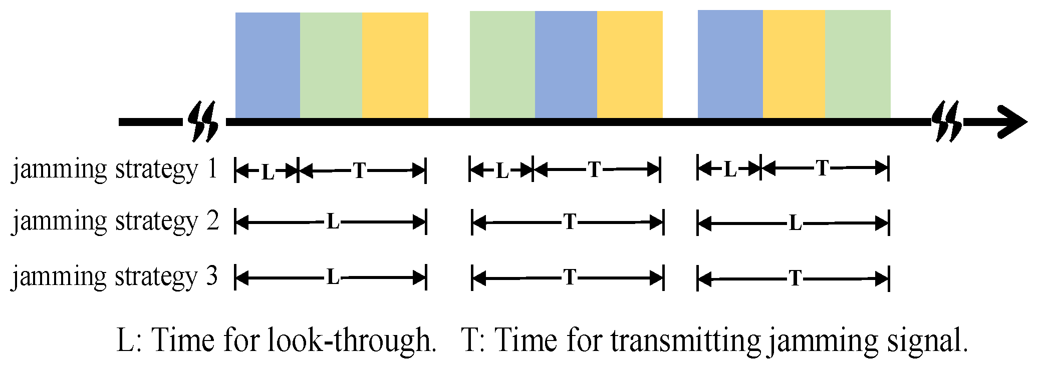
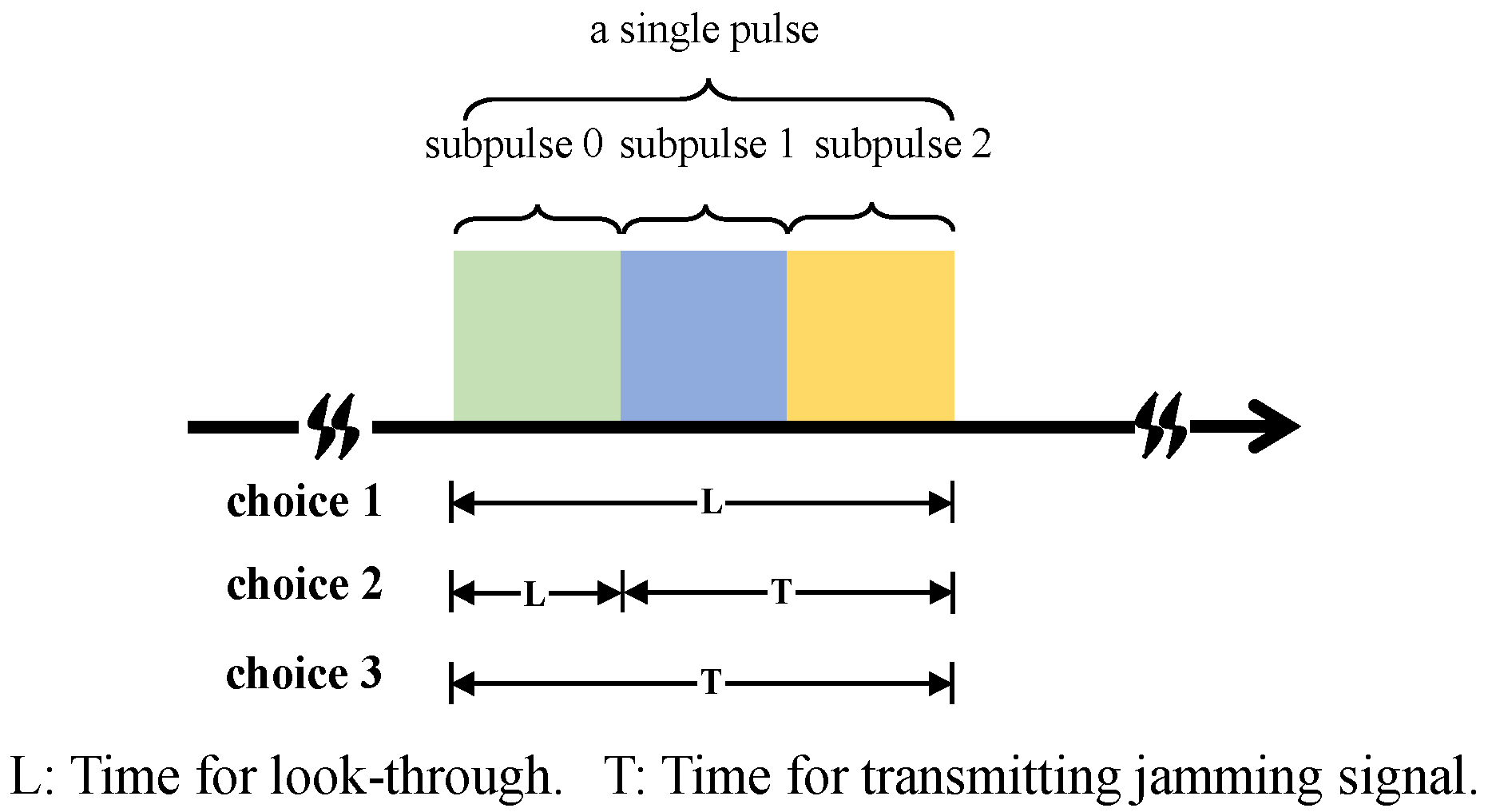
- Choice 1: The jammer performs the look-through operation throughout the whole pulse, which means that the jammer does not transmit a jamming signal and just intercepts the radar waveform;
- Choice 2: The jammer performs the look-through operation for a short period, and then, the jammer transmits a spot jamming signal with a central carrier frequency of or a barrage jamming signal;
- Choice 3: The jammer does not perform the look-through operation and just transmits a spot jamming signal with a central carrier frequency of or a barrage jamming signal.
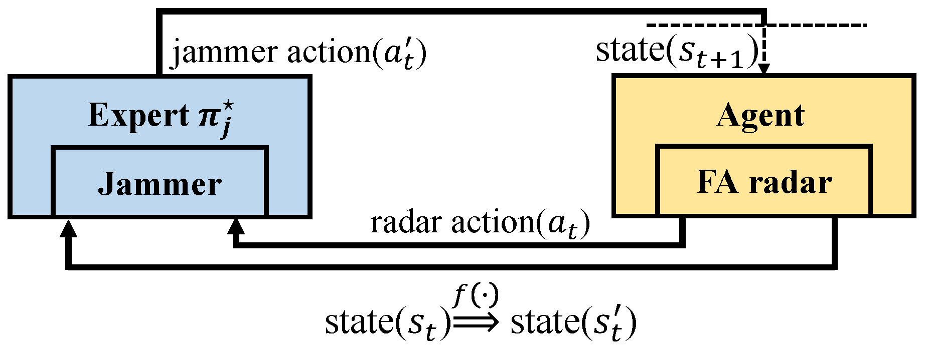
3.2. RL Formulation of the Anti-Jamming Strategy Problem
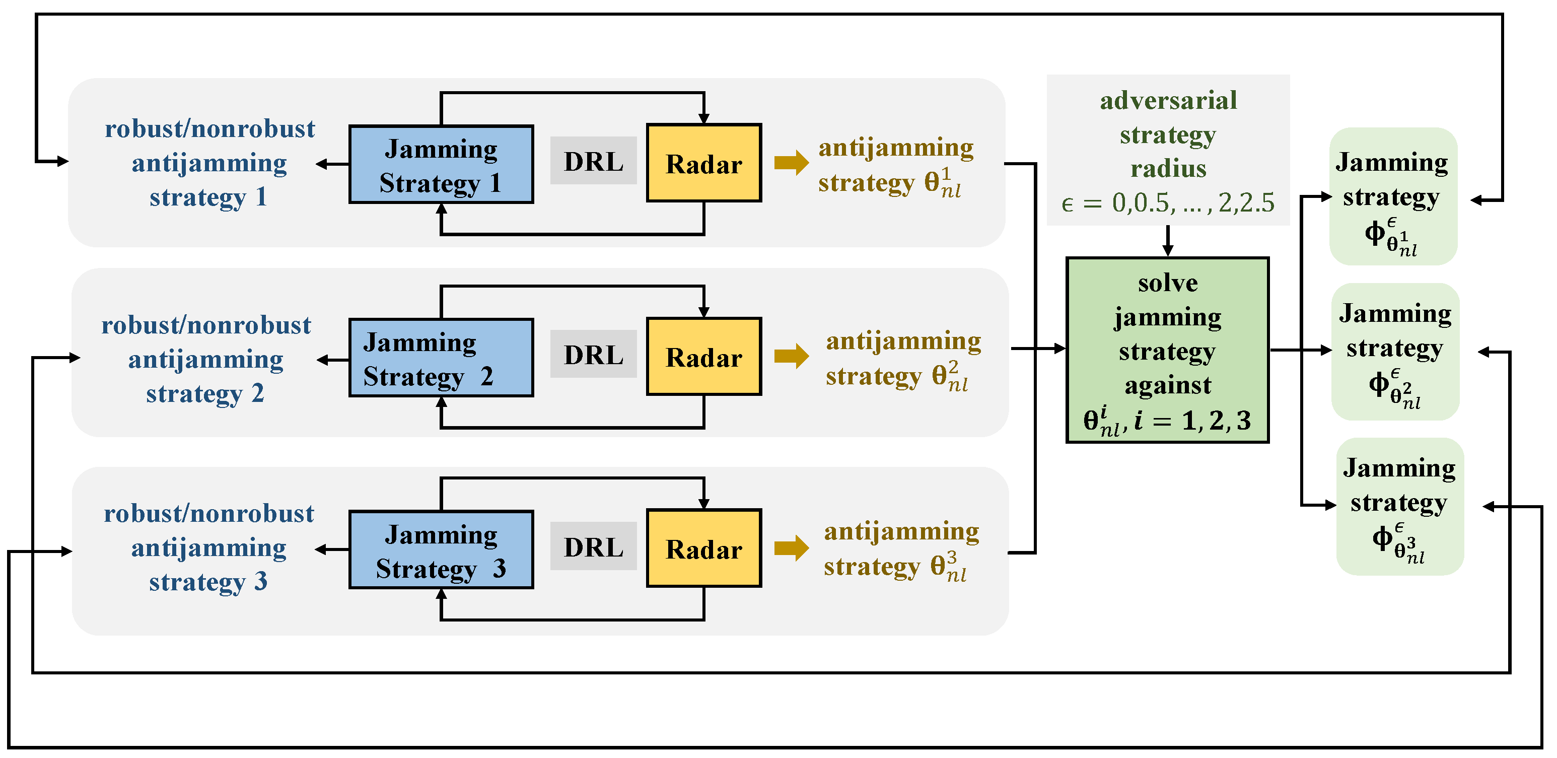
4. Radar Robust Antijamming Strategy Design
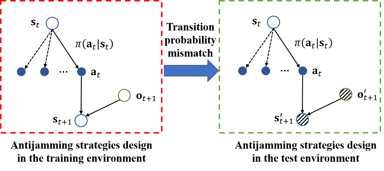
4.1. Robust Formulation
- (1)
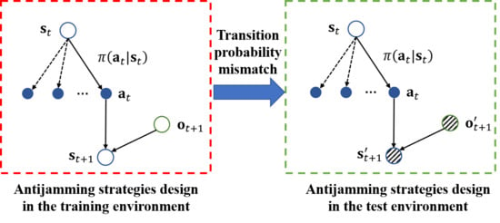
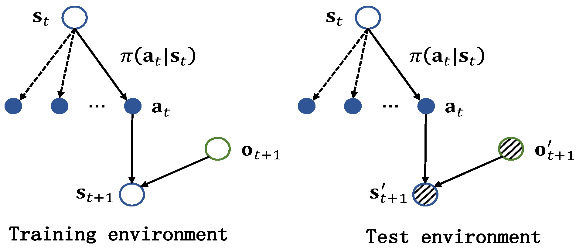
- The dynamic parameters remain unknown for a given jamming strategy, and we can only describe it using predefined rules. For example, a jamming strategy can be expressed by the following rule: the jammer transmits a spot jamming signal whose central frequency is based on the last intercepted radar pulse. Therefore, we proposed a method of imitation learning-based jamming strategy parameterization, as presented in Section 4.2, which aims to express the jamming strategy mathematically;
- (2)
- After jamming strategy parameterization, the jamming strategy can be expressed in a neural network consisting of a series of parameters. As is shown later, the number of parameters of this neural network is large, which will lead to a heavy computational burden. Thus, a jamming parameter perturbation method is provided in Section 4.3 to alleviate this problem.
4.2. Jamming Strategy Parameterization
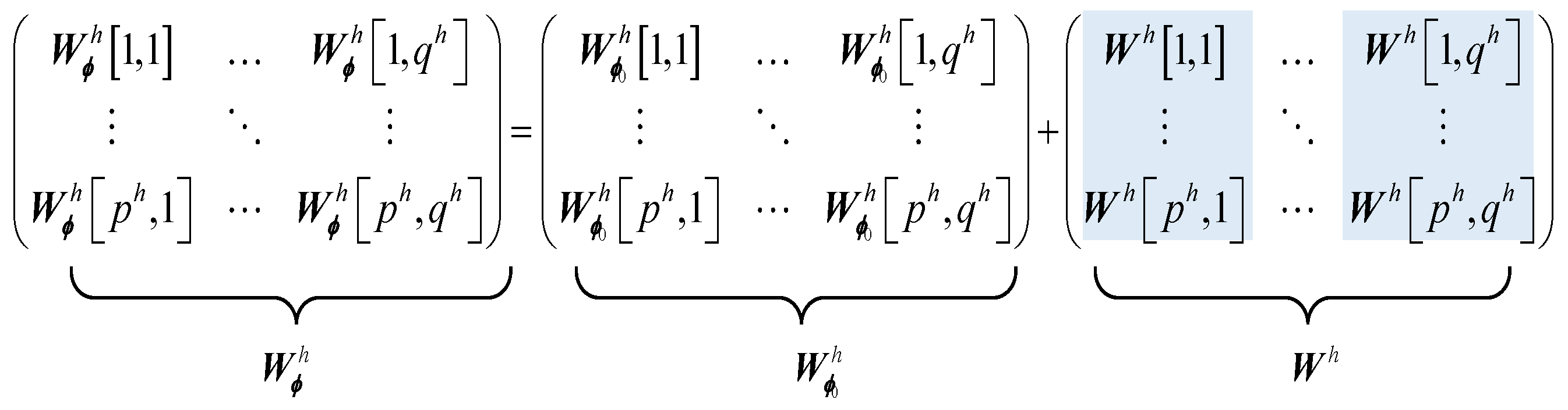
4.3. Jamming Parameter Perturbation
| Algorithm 1: Jamming strategy parameterization. |
| Input: Predefined jamming strategy, mapping function , the number of pulses in one CPI T, the number of trajectories to be collected , the initial parameters of and as , , predefined radar policy , an empty list Output: The parameters of when GAIL is convergent |
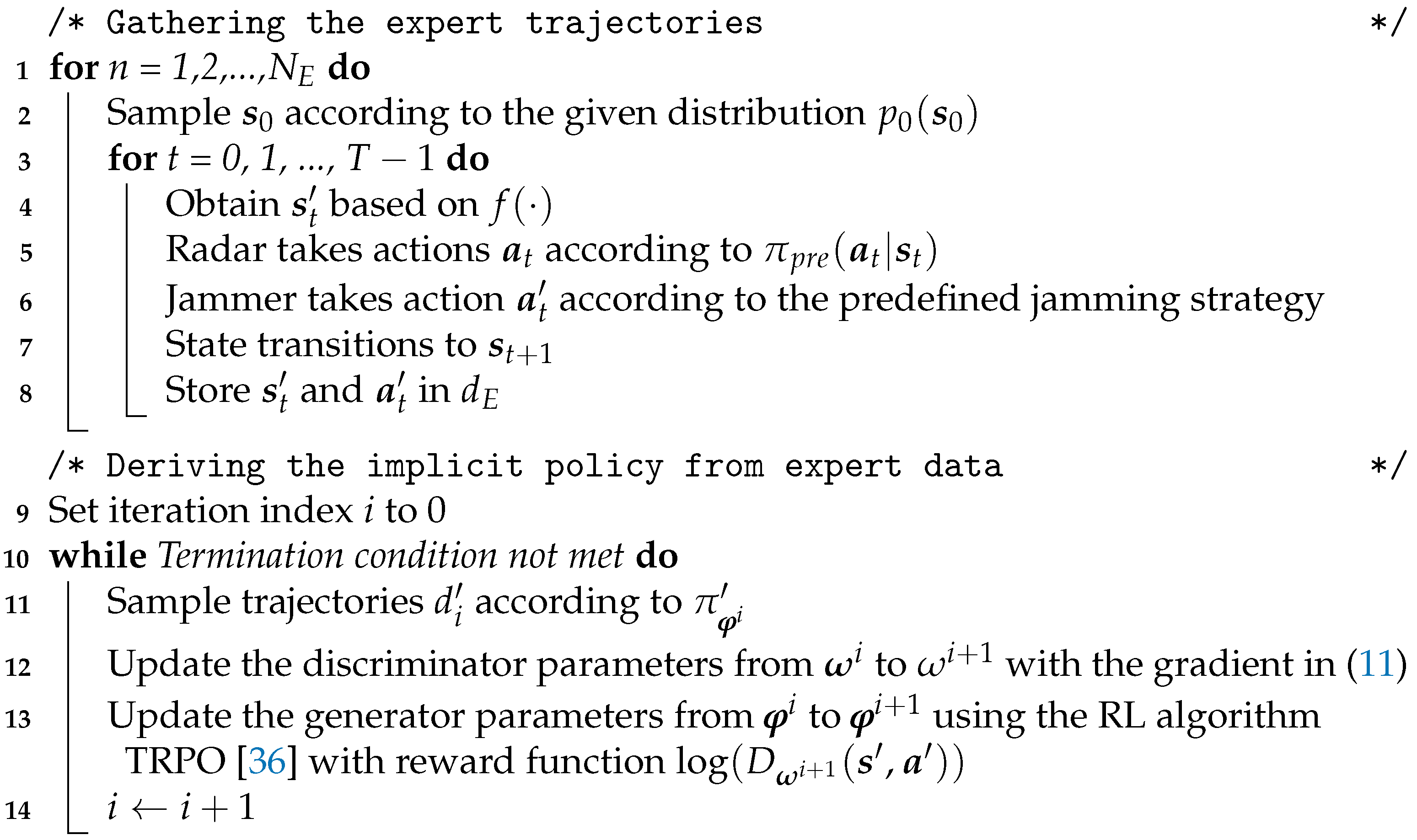 |
4.4. -Based Robust Anti-Jamming Strategy Design
5. Simulation Results
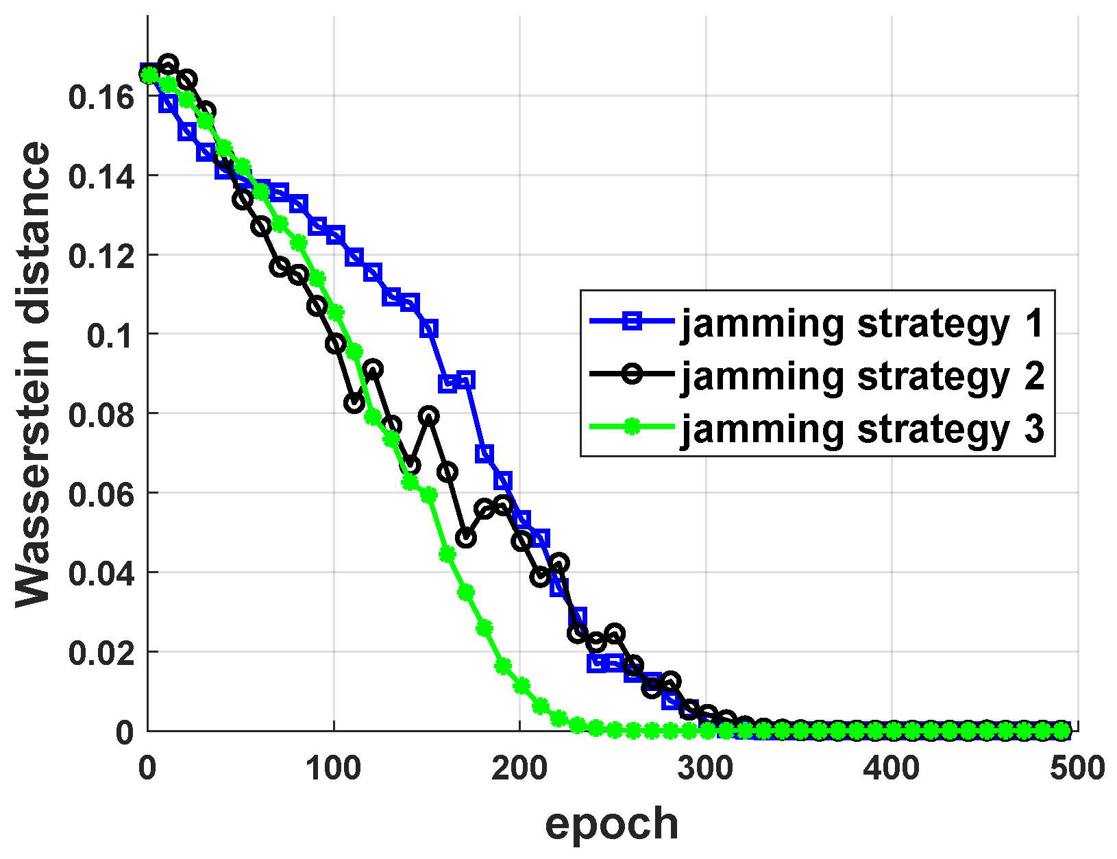
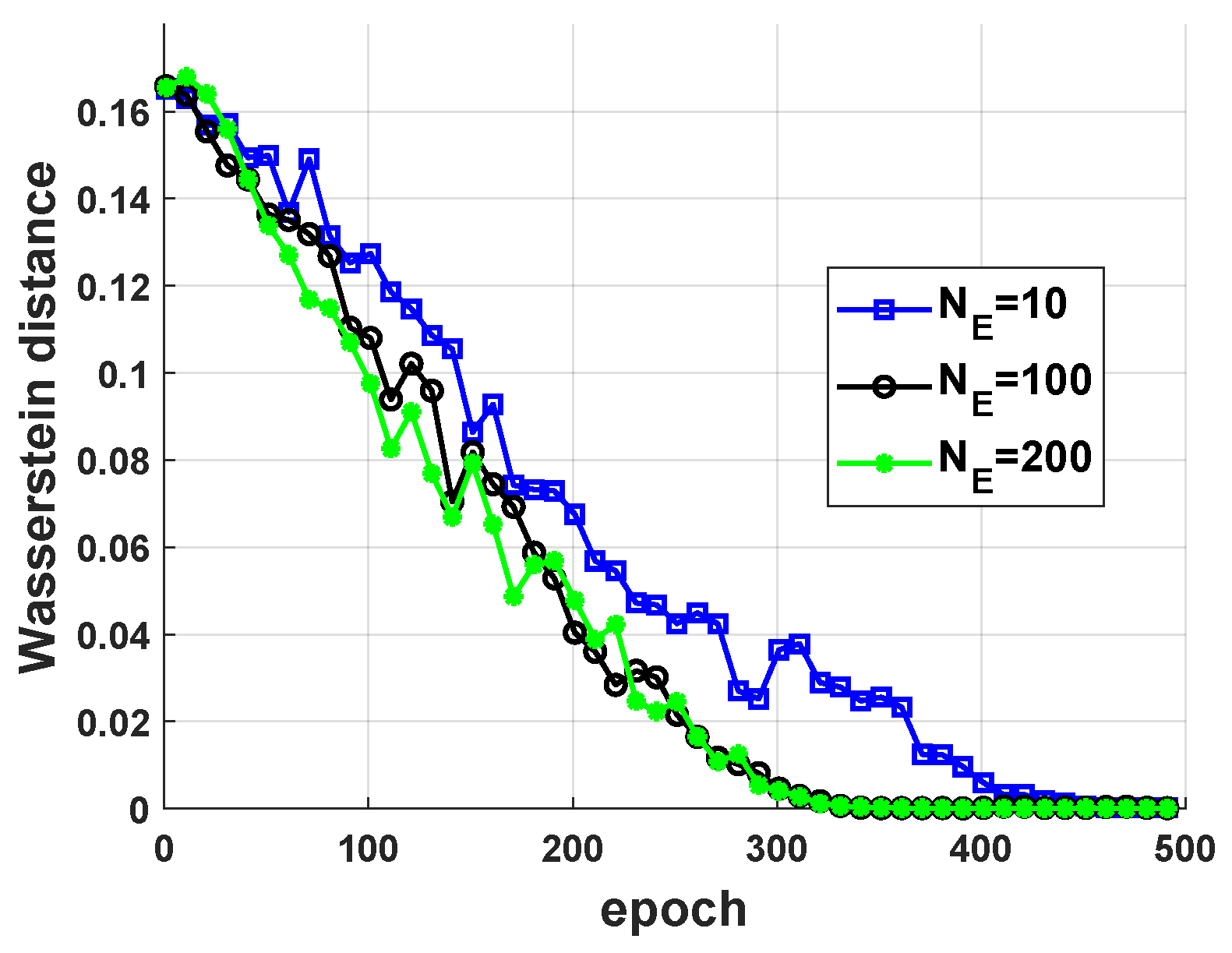
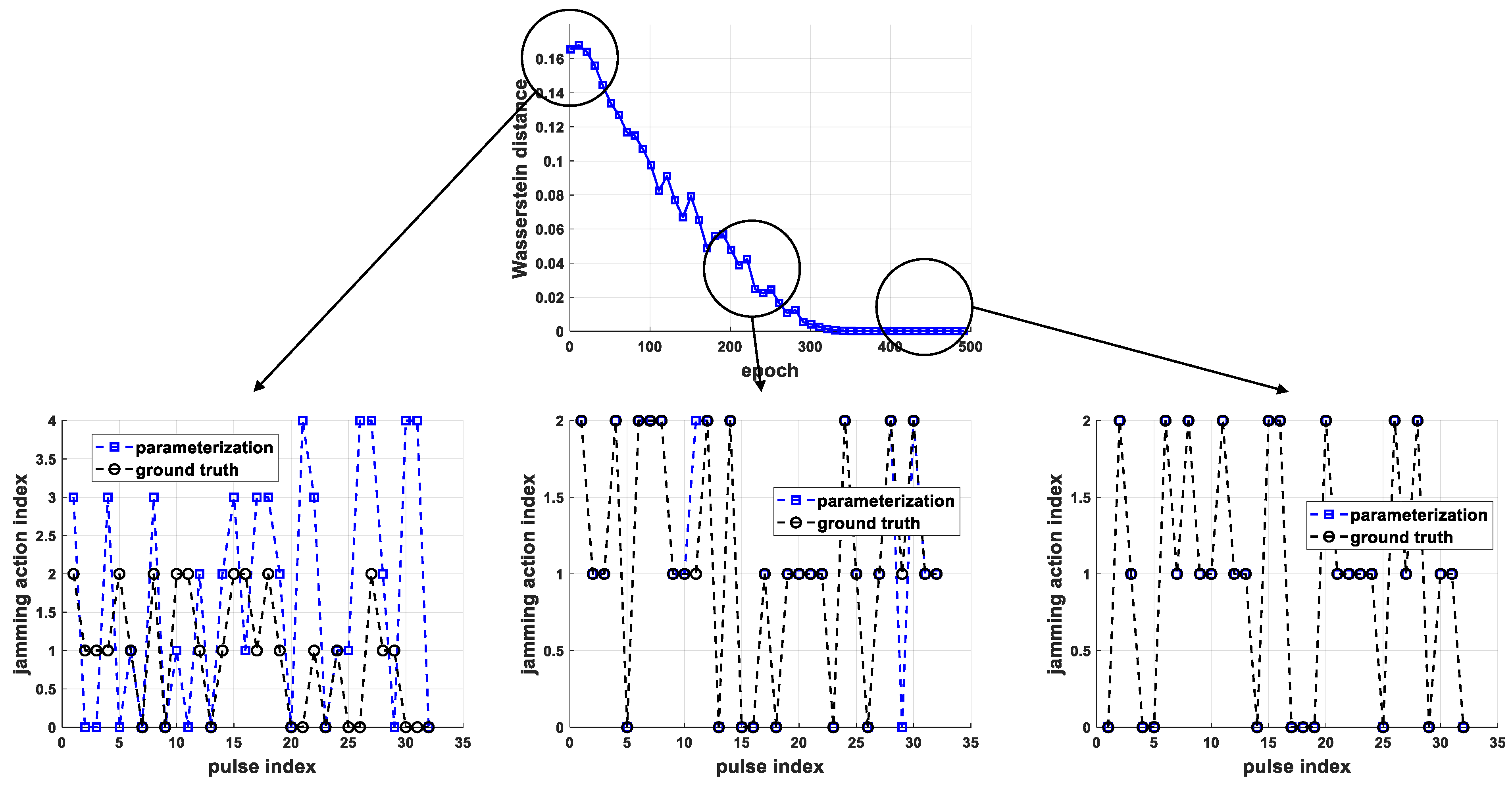
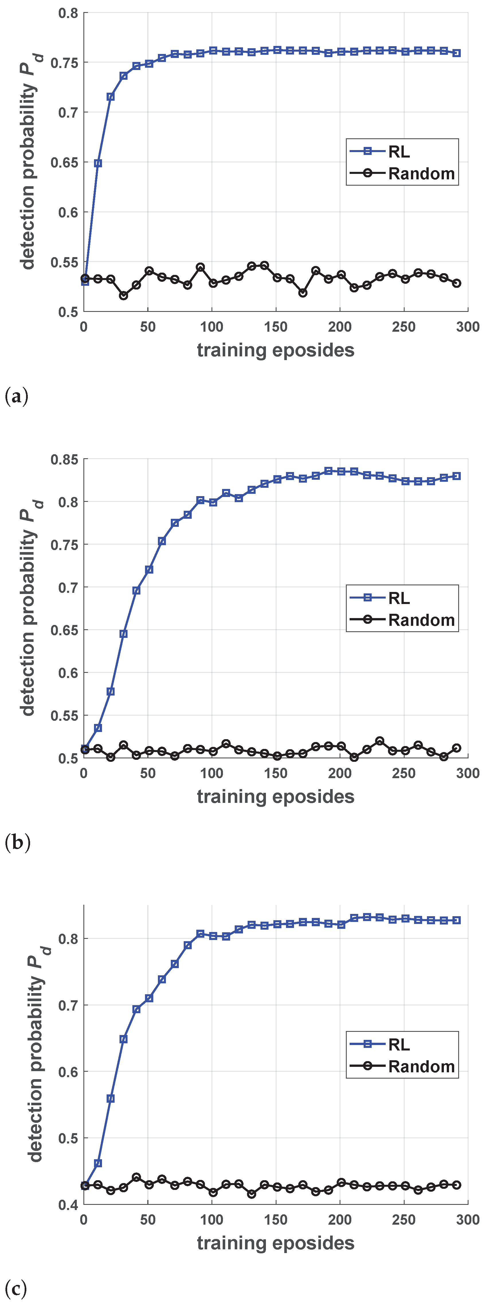
5.1. Performance of Jamming Strategy Parameterization
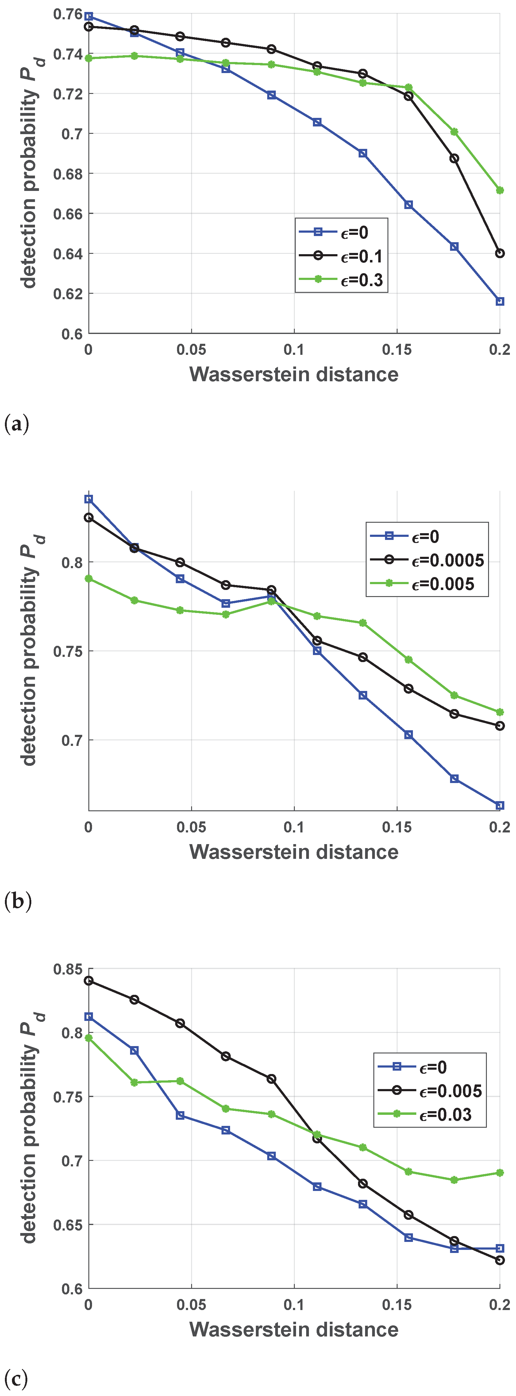
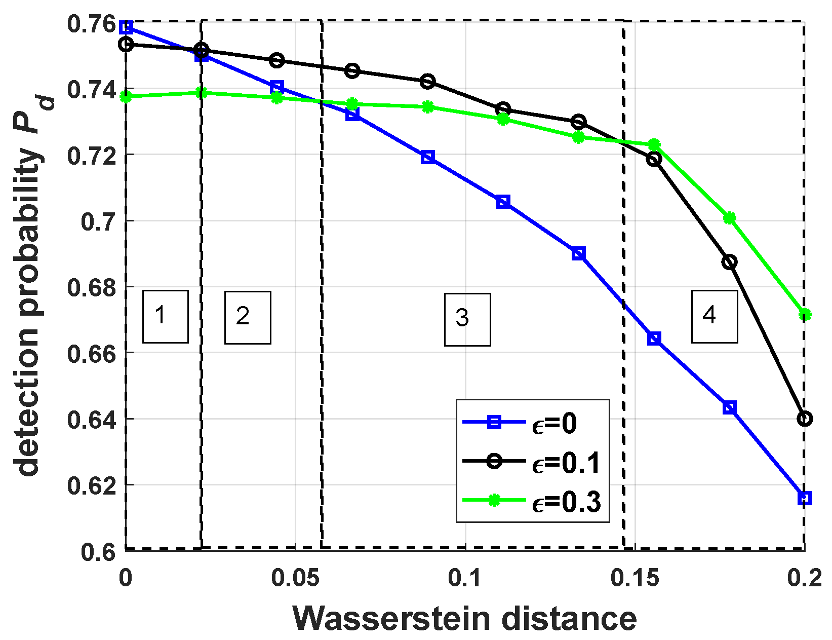
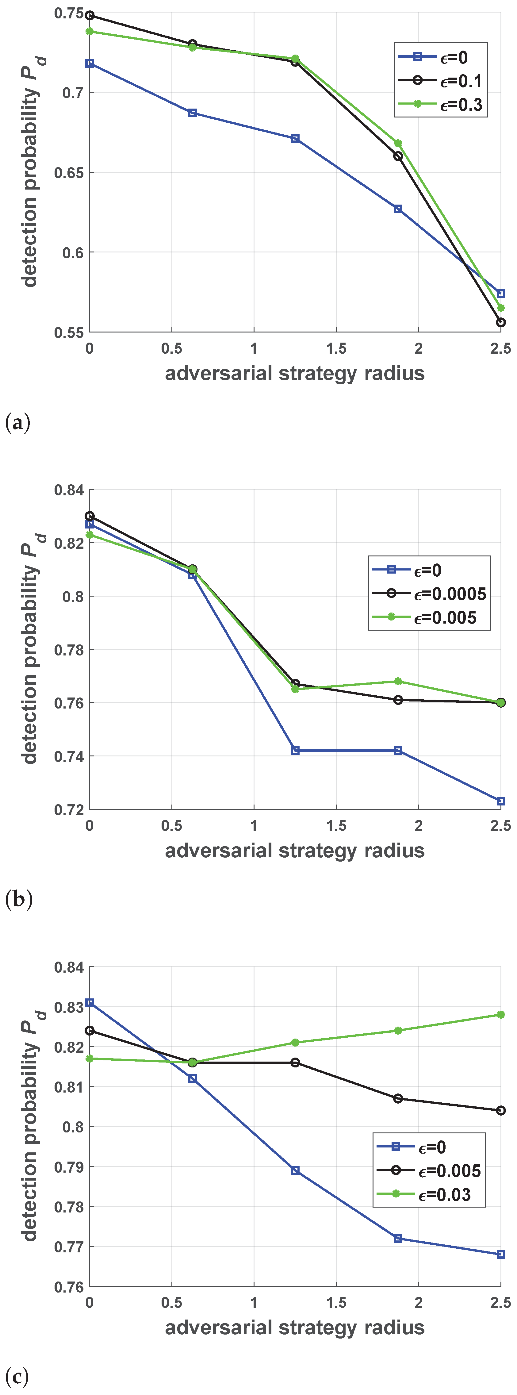
5.2. Performance of Robust Antijamming Strategy Design
6. Conclusions
Author Contributions
Funding
Conflicts of Interest
Appendix A. Calculation of the Probability of Detection
References
- Su, B.; Wang, Y.; Zhou, L. A main lobe interference cancelling method. In Proceedings of the 2005 IEEE International Symposium on Microwave, Antenna, Propagation and EMC Technologies for Wireless Communications, Beijing, China, 8–12 August 2005; Volume 1, pp. 23–26. [Google Scholar]
- Luo, Z.; Wang, H.; Lv, W.; Tian, H. Main lobe Anti-Jamming via Eigen-Projection Processing and Covariance Matrix Reconstruction. IEICE Trans. Fundam. Electron. Commun. Comput. Sci. 2017, E100.A, 1055–1059. [Google Scholar]
- Ge, M.; Cui, G.; Yu, X.; Huang, D.; Kong, L. Main lobe jamming suppression via blind source separation. In Proceedings of the 2018 IEEE Radar Conference (RadarConf18), Oklahoma City, OK, USA, 23–27 April 2018; pp. 914–918. [Google Scholar]
- Neri, F. Introduction to Electronic Defense Systems; SciTech Publishing: Boston, MA, USA, 2006. [Google Scholar]
- Axelsson, S.R.J. Analysis of Random Step Frequency Radar and Comparison With Experiments. IEEE Trans. Geosci. Remote Sens. 2007, 45, 890–904. [Google Scholar]
- Quan, Y.; Wu, Y.; Li, Y.; Sun, G.; Xing, M. Range-Doppler reconstruction for frequency agile and PRF-jittering radar. IET Radar Sonar Navig. 2018, 12, 348–352. [Google Scholar]
- Akhtar, J. Orthogonal Block Coded ECCM Schemes Against Repeat Radar Jammers. IEEE Trans. Aerosp. Electron. Syst. 2009, 45, 1218–1226. [Google Scholar]
- Zhou, R.; Xia, G.; Zhao, Y.; Liu, H. Coherent signal processing method for frequency-agile radar. In Proceedings of the 2015 12th IEEE International Conference on Electronic Measurement Instruments (ICEMI), Qingdao, China, 16–18 July 2015; Volume 1, pp. 431–434. [Google Scholar]
- Bică, M.; Koivunen, V. Generalized multicarrier radar: Models and performance. IEEE Trans. Signal Process. 2016, 64, 4389–4402. [Google Scholar]
- Kang, L.; Bo, J.; Hongwei, L.; Siyuan, L. Reinforcement Learning based Anti-jamming Frequency Hopping Strategies Design for Cognitive Radar. In Proceedings of the 2018 IEEE International Conference on Signal Processing, Communications and Computing (ICSPCC), Qingdao, China, 14–16 September 2018; pp. 1–5. [Google Scholar]
- Li, K.; Jiu, B.; Liu, H. Deep Q-Network based Anti-Jamming Strategy Design for Frequency Agile Radar. In Proceedings of the 2019 International Radar Conference (RADAR), Toulon, France, 23–27 September 2019; pp. 1–5. [Google Scholar]
- Schulman, J.; Wolski, F.; Dhariwal, P.; Radford, A.; Klimov, O. Proximal policy optimization algorithms. arXiv 2017, arXiv:1707.06347. [Google Scholar]
- Ak, S.; Brüggenwirth, S. Avoiding Jammers: A Reinforcement Learning Approach. In Proceedings of the 2020 IEEE International Radar Conference (RADAR), Florence, Italy, 21–25 September 2020; pp. 321–326. [Google Scholar]
- Naparstek, O.; Cohen, K. Deep Multi-User Reinforcement Learning for Dynamic Spectrum Access in Multichannel Wireless Networks. In Proceedings of the GLOBECOM 2017—2017 IEEE Global Communications Conference, Singapore, 4–8 December 2017; pp. 1–7. [Google Scholar]
- Xiao, L.; Jiang, D.; Xu, D.; Zhu, H.; Zhang, Y.; Poor, H.V. Two-Dimensional Antijamming Mobile Communication Based on Reinforcement Learning. IEEE Trans. Veh. Technol. 2018, 67, 9499–9512. [Google Scholar]
- Li, K.; Jiu, B.; Wang, P.; Liu, H.; Shi, Y. Radar Active Antagonism through Deep Reinforcement Learning: A Way to Address the Challenge of Main lobe Jamming. Signal Process. 2021, 2021, 108130. [Google Scholar]
- De Martino, A. Introduction to Modern EW Systems; Artech House: Norwood, MA, USA, 2018. [Google Scholar]
- Stinco, P.; Greco, M.; Gini, F.; Himed, B. Cognitive radars in spectrally dense environments. IEEE Aerosp. Electron. Syst. Mag. 2016, 31, 20–27. [Google Scholar]
- Hussein, A.; Gaber, M.M.; Elyan, E.; Jayne, C. Imitation learning: A survey of learning methods. ACM Comput. Surv. 2017, 50, 1–35. [Google Scholar]
- Abdullah, M.A.; Ren, H.; Ammar, H.B.; Milenkovic, V.; Luo, R.; Zhang, M.; Wang, J. Wasserstein robust reinforcement learning. arXiv 2019, arXiv:1907.13196. [Google Scholar]
- Sutton, R.S.; Barto, A.G. Reinforcement Learning: An Introduction; MIT Press: Cambridge, MA, USA, 2011. [Google Scholar]
- Pinto, L.; Davidson, J.; Sukthankar, R.; Gupta, A. Robust Adversarial Reinforcement Learning. In Proceedings of the International Conference on Machine Learning, Sydney, Australia, 6–11 August 2017; pp. 2817–2826. [Google Scholar]
- Rajeswaran, A.; Ghotra, S.; Ravindran, B.; Levine, S. EPOpt: Learning Robust Neural Network Policies Using Model Ensembles. In Proceedings of the 5th International Conference on Learning Representations, ICLR 2017, Toulon, France, 24–26 April 2017. [Google Scholar]
- Abbeel, P.; Ng, A.Y. Apprenticeship learning via inverse reinforcement learning. In Proceedings of the Twenty-First International Conference on Machine learning, Banff, AB, Canada, 4–8 July 2004. [Google Scholar]
- Ho, J.; Ermon, S. Generative adversarial imitation learning. In Advances in Neural Information Processing Systems; Curran Associates, Inc.: Red Hook, NY, USA, 2016; pp. 4565–4573. [Google Scholar]
- Ross, S.; Bagnell, D. Efficient Reductions for Imitation Learning. In Proceedings of the Thirteenth International Conference on Artificial Intelligence and Statistics; Teh, Y.W., Titterington, M., Eds.; Proceedings of Machine Learning Research; PMLR: Sardinia, Italy, 2010; Volume 9, pp. 661–668. [Google Scholar]
- Huang, T.; Liu, Y.; Meng, H.; Wang, X. Cognitive random stepped frequency radar with sparse recovery. IEEE Trans. Aerosp. Electron. Syst. 2014, 50, 858–870. [Google Scholar]
- Adamy, D. EW 101: A First Course in Electronic Warfare; Artech House: Norwood, MA, USA, 2001; Volume 101. [Google Scholar]
- Richards, M.A. Fundamentals of Radar Signal Processing; Tata McGraw-Hill Education: New Delhi, India, 2005. [Google Scholar]
- Liu, H.; Zhou, S.; Su, H.; Yu, Y. Detection performance of spatial-frequency diversity MIMO radar. IEEE Trans. Aerosp. Electron. Syst. 2014, 50, 3137–3155. [Google Scholar]
- Brockman, G.; Cheung, V.; Pettersson, L.; Schneider, J.; Schulman, J.; Tang, J.; Zaremba, W. OpenAI Gym. arXiv 2016, arXiv:1606.01540. [Google Scholar]
- Nesterov, Y.; Spokoiny, V. Random gradient-free minimization of convex functions. Found. Comput. Math. 2017, 17, 527–566. [Google Scholar]
- Argall, B.D.; Chernova, S.; Veloso, M.; Browning, B. A survey of robot learning from demonstration. Robot. Auton. Syst. 2009, 57, 469–483. [Google Scholar]
- Ng, A.Y.; Russell, S.J. Algorithms for inverse reinforcement learning. Icml 2000, 1, 2. [Google Scholar]
- Goodfellow, I.; Pouget-Abadie, J.; Mirza, M.; Xu, B.; Warde-Farley, D.; Ozair, S.; Courville, A.; Bengio, Y. Generative adversarial nets. In Proceedings of the Advances in Neural Information Processing Systems, Montreal, QC, Canada, 8–11 December 2014; pp. 2672–2680. [Google Scholar]
- Schulman, J.; Levine, S.; Abbeel, P.; Jordan, M.; Moritz, P. Trust region policy optimization. In Proceedings of the International Conference on Machine Learning, Lille, France, 6–11 July 2015; pp. 1889–1897. [Google Scholar]
- Fortunato, M.; Azar, M.G.; Piot, B.; Menick, J.; Hessel, M.; Osband, I.; Graves, A.; Mnih, V.; Munos, R.; Hassabis, D.; et al. Noisy Networks For Exploration. In Proceedings of the International Conference on Learning Representations, Vancouver, BC, Canada, 30 April–3 May 2018. [Google Scholar]
- Salimans, T.; Ho, J.; Chen, X.; Sidor, S.; Sutskever, I. Evolution strategies as a scalable alternative to reinforcement learning. arXiv 2017, arXiv:1703.03864. [Google Scholar]
- Chen, T.; Liu, J.; Xiao, L.; Huang, L. Anti-jamming transmissions with learning in heterogenous cognitive radio networks. In Proceedings of the 2015 IEEE Wireless Communications and Networking Conference Workshops (WCNCW), New Orleans, LA, USA, 9–12 March 2015; pp. 293–298. [Google Scholar]
- Castano-Martinez, A.; Lopez-Blazquez, F. Distribution of a sum of weighted central chi-square variables. Commun. Stat. Theory Methods 2005, 34, 515–524. [Google Scholar]


| Parameter | Value |
|---|---|
| radar transmitter power | 30 kW |
| radar transmit antenna gain | 30 dB |
| radar initial frequency | 3 GHz |
| bandwidth of each subpulse B | 2 MHz |
| the number of subpulses in a single pulse | 3 |
| the number of frequencies available for the radar | 3 |
| the number of pulses in one CPI | 32 |
| distance between the radar and the jammer | 100 km |
| false alarm rate | |
| the length of the target along the radar boresight l | 10 m |
| jammer transmitter power | 1 W |
| jammer transmit antenna gain | 0 dB |
Publisher’s Note: MDPI stays neutral with regard to jurisdictional claims in published maps and institutional affiliations. |
© 2021 by the authors. Licensee MDPI, Basel, Switzerland. This article is an open access article distributed under the terms and conditions of the Creative Commons Attribution (CC BY) license (https://creativecommons.org/licenses/by/4.0/).
Share and Cite
Li, K.; Jiu, B.; Liu, H.; Pu, W. Robust Antijamming Strategy Design for Frequency-Agile Radar against Main Lobe Jamming. Remote Sens. 2021, 13, 3043. https://doi.org/10.3390/rs13153043
Li K, Jiu B, Liu H, Pu W. Robust Antijamming Strategy Design for Frequency-Agile Radar against Main Lobe Jamming. Remote Sensing. 2021; 13(15):3043. https://doi.org/10.3390/rs13153043
Chicago/Turabian StyleLi, Kang, Bo Jiu, Hongwei Liu, and Wenqiang Pu. 2021. "Robust Antijamming Strategy Design for Frequency-Agile Radar against Main Lobe Jamming" Remote Sensing 13, no. 15: 3043. https://doi.org/10.3390/rs13153043
APA StyleLi, K., Jiu, B., Liu, H., & Pu, W. (2021). Robust Antijamming Strategy Design for Frequency-Agile Radar against Main Lobe Jamming. Remote Sensing, 13(15), 3043. https://doi.org/10.3390/rs13153043