Abstract
Fine particulate matter in the lower atmosphere (PM2.5) continues to be a major public health problem globally. Identifying the key contributors to PM2.5 pollution is important in monitoring and managing atmospheric quality, for example, in controlling haze. Previous research has been aimed at quantifying the relationship between PM2.5 values and their underlying factors, but the spatial and temporal dynamics of these factors are not well understood. Based on random forest and Shapley additive explanation (SHAP) algorithms, this study analyses the spatiotemporal variations in selected key factors influencing PM2.5 in Zhejiang Province, China, for the period 2000–2019. The results indicate that, while factors influencing PM2.5 varied significantly during the period studied, SHAP values suggest that there is consistency in their relative importance as follows: meteorological factors (e.g., atmospheric pressure) > socioeconomic factors (e.g., gross domestic product, GDP) > topography and land cover factors (e.g., elevation). The contribution of GDP and transportation factors initially increased but has declined in the recent past, indicating that economic and infrastructural development does not necessarily result in increased PM2.5 concentrations. Vegetation productivity, as indicated by changes in NDVI, is demonstrated to have become more important in improving air quality, and the area of the province over which it constrains PM2.5 concentrations has increased between 2000 and 2019. Mapping of SHAP values suggests that, although the relative importance of industrial emissions has declined during the period studied, the actual area positively impacted by such emissions has actually increased. Despite developments in government policy, greater efforts to conserve energy and reduce emissions are still needed. The study further demonstrates that the combination of random forest and SHAP methods provides a valuable means to identify regional differences in key factors affecting atmospheric PM2.5 values and offers a reliable reference for pollution control strategies.
1. Introduction
Urbanization, industrialization, and other human activities, coupled with climate change, have greatly affected air quality [1,2,3,4,5]. Fine particulate matter with an aerodynamic diameter of less than 2.5 μm, known as PM2.5, may be suspended in the atmosphere for a considerable period and can be transported over long distances [6]. In addition to their direct effect on the respiratory tract, these aerosols may absorb toxic substances, which further intensify their negative impact on human health [7,8,9]. Persistent PM2.5 pollution is a serious environmental problem [10,11,12] that has secondary implications for potential economic investment, the tourism industry and threatens sustainable development [13].
There are numerous studies aimed at identifying and quantifying the major factors influencing PM2.5 concentrations. It is widely accepted that meteorological conditions, e.g., sunshine duration [14], temperature [15], precipitation [16], atmospheric pressure [17], and wind speed [18], play important roles in the long-term dispersion and deposition of PM2.5. Topography and land cover also have strong effects on the diffusion of PM2.5 [19]. Moreover, socioeconomic factors (e.g., per capita GDP [20], population density [21], and industrialization [22]) are known to have a marked influence on PM2.5 concentrations. Nevertheless, rather little is known about how such influencing factors vary over time and between regions, so comprehensive and systematic research to reveal the spatiotemporal dynamics of PM2.5 concentrations and its relationship with influencing factors is warranted.
Simulation models and statistical methods have been used in the past to clarify the potential relations among PM2.5-related factors [23,24]. For example, chemical transport models (CTMs) are effective in simulating interactions between PM2.5 and meteorological factors [25]. However, these require complex calculations involving multiple parameters and have proved very challenging to apply [26]. Statistical methods, such as stepwise regression [27], geographical detector modeling [28], and geographically weighted regression (GWR) [29,30], have also been applied to retrieve regional scale PM2.5 values. Despite claims of operability and ease of interpretation, however, performance has proved to be variable due to the complexity of processes controlling PM2.5 genesis, transport, and deposition, and the application of GWR, for example, appears to be associated with considerable uncertainty [26]. Moreover, statistical models are sensitive to the multicollinearity problem [31], which reduces the accuracy of the estimated value, resulting in difficulties regarding the influence of the independent variable on the dependent variable. Machine learning methods, such as neural networks and random forest, overcome this limitation and obtain more accurate predictions by learning from the given dataset even when faced with highly complex relationships [32,33]. Machine learning modeling is, however, a black box approach in which it is not possible to fully account for the relative importance of key contributors to spatial-temporal variations, such as in PM2.5. Using the Shapley additive explanation (SHAP) algorithm overcomes this challenge by recovering both the direction and relative importance of influencing variables within a spatial unit [34,35], and therefore offers a potentially valuable approach to investigating the factors underlying the spatiotemporal dynamics of PM2.5.
Given the importance of aerosol pollution in terms of ecological security and sustainable development, and considering the flexibility of machine learning methods, the aim of this study is to use random forest regression and SHAP algorithms to reveal, using data from Zhejiang Province, China, the relative importance of selected variables in the spatiotemporal dynamics of PM2.5 for the period 2000–2019. The main objectives of this study are: (1) identify key factors affecting PM2.5 pollution in the study area; (2) reveal changes in the relative influence of these factors over time; (3) provide a scientific basis for more accurate regional PM2.5 prediction and pollution management.
2. Materials and Methods
2.1. Study Region
Zhejiang Province (27°12′N–31°31′N, 118°01′E–123°10′E), lies to the south of the Yangtze River Delta in southeastern China (Figure 1) and forms an important part of the large urban agglomeration in China [36,37]. The province is characterized by a subtropical monsoon climate with mean annual temperature between 15 °C and 18 °C, and mean annual precipitation between 1000 and 2000 mm [38]. Straddling the Jinqu basin in the central part of the province are the more mountainous areas to the southwest and the coastal plains which characterize the north [39]. Although the province only occupies 105,500 km2 and accounts for just 1.1% of the total area of the country, its permanent population reached 58.5 million in 2019 with an annual gross regional production value of more than 6 billion CNY (Zhejiang Statistical Yearbook 2020). As a result of rapid urbanization and industrialization, with economic growth based on energy derived largely from fossil fuel, the region is associated with significant PM2.5-related problems [40]. The entire province has experienced persistent air pollution since the 1970s, and there are frequent occurrences of severe smog, for example the extreme event of December 2013 that lasted several weeks [41].
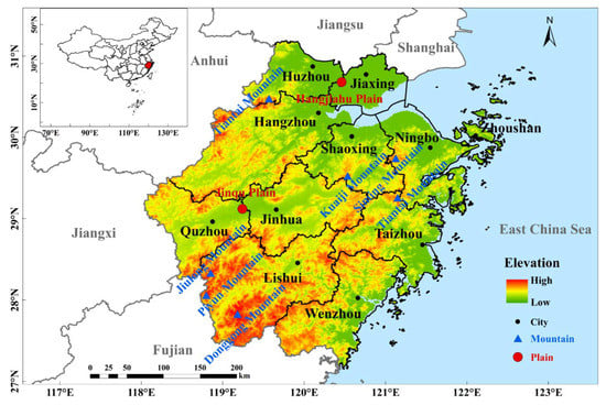
Figure 1.
Map of Zhejiang province in China.
2.2. Data Sources
Five types of data were used, including atmospheric PM2.5 data, meteorological data, topography and land cover data (including a vegetation index), socioeconomic data, and administrative boundaries (Table 1).

Table 1.
Variables used in this study.
- (1)
- PM2.5 data retrieved from remote sensing imageries. Considering the fact that the monitoring stations in China were established in 2013, satellite-based aerosol optical depth (AOD) data with abundant historic archives were adopted. Researchers have found a high correlation between AOD and observed PM2.5 measurements, in addition to its advantages of low cost, wide spatial coverage, and high simulation accuracy [42]. The satellite-derived PM2.5 concentrations (µg/m3) dataset for China is freely available from the Hong Kong University of Science and Technology at: http://envf.ust.hk/dataview/aod2pm/current/ (accessed on 20 April 2021) and has been regularly utilized in studies of air pollution [43]. The PM2.5 data at a spatial resolution of 0.03° × 0.03° were obtained in this study for the period 2000 to 2019 (Due to the lack of PM2.5 data in parts of eastern Zhejiang province, Zhoushan city is omitted from the study), and the PM2.5 concentration below refers to the annual average value.
- (2)
- Meteorological data. The datasets were sourced from the “Daily Surface Climate Variables of China” catalog, which is released by the Climatic Data Center, National Meteorological Information Center, China Meteorological Administration and China Meteorological Data Sharing Service System (http://data.cma.cn, accessed on 20 May 2021). The extensive dataset runs from 1 January 1951 and maintains records of 699 observation stations throughout mainland China. We selected mean daily air temperature (TEM), atmospheric pressure (PRS), relative humidity (RHU), wind speed (WIN), ground temperature (GST), sunshine duration (SSD), and total precipitation (PRE) as the main variables. The dataset was handled to annual data. Raster/grid maps for the respective values were produced at 1 km resolution using the thin plate spline spatial interpolation method combined with topographic correction based on digital elevation models (DEM), which is produced from the Shuttle Radar Topography Mission (SRTM) data [44].
- (3)
- Topography and land cover data. The normalized difference vegetation index (NDVI) is frequently used as a standard indicator of vegetation growth state. Elevation, NDVI, and land cover data were obtained from the Resource and Environment Science and Data Center (RESDC) (http://www.resdc.cn, accessed on 20 May 2021). Elevation and mean annual NDVI grid data are both 1 km × 1 km resolution. Land cover (Land cover data for 2020 were used due to the lack of 2019 data) was simplified from 26 classes into five classes, viz., farmland, woodland, grassland, water body, and construction land. The proportion of each land use type was calculated based on a 3 km × 3 km rectangular buffer zone extracted from the centered sampling point value.
- (4)
- Socioeconomic data. We selected data for GDP, population density, proportion of primary, secondary, tertiary and total industry, highway mileage, passenger volume, freight volume, car ownership, industrial waste gas emissions, industrial sulfur dioxide emissions, industrial smoke (dust) emissions, electricity consumption, and energy consumption. All values were extracted from the Zhejiang Province statistical yearbook (2001–2020) and the China Urban Statistical Yearbook (2001–2020) (http://tjj.zj.gov.cn, accessed on 15 May 2021).
- (5)
- Other data. The administrative boundary for Zhejiang Province was derived from the 1:1 million basic geographic databases of the National Catalogue Service for Geographic Information (http://www.webmap.cn, accessed on 20 April 2021).
All data values were normalized to the same coordinates and spatial resolution of 3 km × 3 km using ArcGIS 10.2. Data for the years 2000, 2005, 2010, 2015, and 2019 were selected as representing the corresponding period 2000 to 2019.
2.3. Methods
2.3.1. Random Forest
Random forest is a machine learning algorithm that uses a combination of several random decision trees, where each tree is generated in a specific way to induce diversity, and all predictions are formed by voting [45]. The bootstrap aggregation technique, known as bagging, is used to achieve higher accuracy and reduce overfitting [46]. In regression, the algorithm takes the average of the individual predictions as the predicted outcome. The random forest method has been shown to be efficient and to provide high levels of predictive accuracy in situations where potential variables have complex relations [47], such as is the case for factors influencing PM2.5 concentrations. In this study, PM2.5 concentration is treated as the response variable, and the explanatory variables are influencing factors.
Parameter selection and adjustment are necessary for random forest to prevent overfitting and minimize complexity. In this study, 10-fold cross-validation was employed to find the most suitable parameters, including the number of trees (n_estimators), the maximum depth of each tree (max_depth), the minimum number of samples to split a node (min_sample_split), and the maximum number of features for the best split (max_features). The grid search mode was used during the process to evaluate model performance [48]. The datasets were randomly divided into 10 subsets; 9 were used as training data, and the other as validation data. This process was repeated 10 times across the dataset, and error rates averaged to obtain the results. Three metrics, viz., mean absolute error (MAE), root mean squared error (RMSE), and the coefficient of determination (R2), were used in this study to evaluate model performance [49]. All models run were conducted in Python with the scikit-learn package.
2.3.2. Shapley Additive Explanation (SHAP)
Machine learning algorithms may yield powerful predictive models, but understanding why a model makes a particular prediction is as important as its accuracy, and the black-box nature of random forest needs to be resolved [44]. To understand the physical mechanisms, Lundberg and Lee [50] proposed Shapley additive explanations (SHAP) based on game theory. SHAP specifies the explanation as follows, in which the explanatory model g is a linear function of the feature attribution:
where z’ ∈ {0, 1}M, and M represents the number of simplified input features. ϕi ∈ R indicates the feature attribution for feature i, the SHAP values. Intuitively, the model g can be used to interpret both a single prediction and the entire model based on the average feature attribution across all the observations, and therefore, the method resolves the relative importance of the various features under consideration.
Before calculating SHAP values, it is necessary to fit one model fS∪{i} involving factor i, and another one, fs, without it. The difference in input x between these models is the marginal contribution of factor i. When more than one factor is being considered, contributions depend on interactions with the other factors such that the procedure is repeated for the complete set (i.e., all possible subsets S ⊆ F including the empty set and the set F of all factors). The final factor contribution ϕi ∈ R is the weighted average of all marginal contributions [51]:
The final model prediction is then obtained by summing up SHAP values for each input feature. SHAP values can be negative since every single SHAP value of each point is calculated relative to the average value. A positive SHAP value means that the prediction (PM2.5) based on the corresponding influencing factor is above the mean value (the average PM2.5). The relative importance of each variable is represented by their mean absolute SHAP values [52]. Advantages of the SHAP algorithm include: (1) global interpretability—the collective SHAP value can identify positive or negative relationships for each variable, and the global importance of different features can be calculated by computing their respective absolute SHAP values; (2) local interpretability—each feature acquires its own corresponding spatial SHAP value in different locations; this resolves the limitation of traditional methods of evaluating relative importance whereby results are obtained across the entire region or population but not for each pixel and individual [53]. Therefore, SHAP values can be used to represent the relative importance of potential influencing factors. Here, the mean absolute SHAP value (global SHAP value) is calculated to describe the importance of each factor for significance comparison, and local SHAP values in different positions are used to demonstrate their spatial contribution variation.
Traditional Shapley regression is time-consuming since a large number of possible feature combinations have to be included. However, faster computation with a high level of accuracy is possible, as in this study, using the SHAP framework with tree-based model. All SHAP values were computed using the “shap” package in Python 3.7.
3. Results
3.1. Spatiotemporal Changes in PM2.5, 2000–2019
Figure 2 graphically summarizes the regional maximum, mean, and minimum values of the annual mean of PM2.5 concentrations in Zhejiang Province. Mean values fluctuated between 35 and 40 μg/m3 until around 2011, whereafter there was a decline that became more marked after 2014. In 2018, mean PM2.5 concentrations fell to their lowest values, followed by a slight increase in 2019. The trend of the maximum value is similar to the mean value, while the minimum value changes slightly, basically fluctuating around 18 μg/m3.
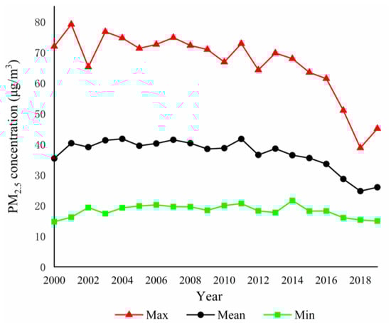
Figure 2.
Maximum (red), mean (black), and minimum (green) values of annual mean of PM2.5 concentrations in Zhejiang Province.
Figure 3 illustrates that the magnitude and spatial distribution of PM2.5 in Zhejiang Province changed markedly between 2000 and 2019. In 2000, the areas with very high pollution levels (i.e., mean annual PM2.5 > 50 μg/m3) were clustered around Hangzhou, situated in the low-lying plains to the north, Quzhou City and Jinhua City in the western basin, and Taizhou City along the southeast coast. By 2005, the highly polluted area around Hangzhou city had extended outwards to its suburbs, while severe pollution in the western basin and southeast coast had also expanded significantly. However, the trend of increase in the areas exposed to high levels of pollution reversed after 2010 such that, by 2019, there were no parts of the province where mean annual PM2.5 values exceeded 50 μg/m3. According to the ambient air quality standards of China (GB3095-2012), mean annual PM2.5 levels greater than 35 μg/m3 represent a health hazard, so it is important to consider the spatiotemporal dynamics of areas where this value is exceeded. Until 2015, areas with values above this threshold were located mainly in the northern parts of the province with the exception of the eastern coastal plain and Tiantai and Siming Mountains in the east, and Tianmu Mountain in the northwest. By 2019, other than in the more industrialized eastern coastal plain areas of Wenzhou and Taizhou, and the Hangjiahu Plain and Jinqu Basin, the province in general experienced mean annual PM2.5 concentrations below 35 μg/m3.
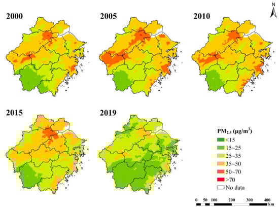
Figure 3.
Spatial distribution map of PM2.5 concentrations in Zhejiang Province for selected years during 2000–2019.
In order to avoid issues of bias and over-fitting in the application of the random forest method, 10-fold cross-validation of the optimal model was repeated 20 times to obtain the final result (Table 2). The coefficient of determination (R2) refers to the strength of the linear relationship between variables. The nearer that R2 is to 1, the more the independent variable can account for variations in the dependent variable. The R2 values for the five selected years exceed 0.96, indicating that the input factors are strongly correlated with the dependent variable (PM2.5). Root mean square error (RMSE) is the square root of the mean square error between the fitted data and corresponding sampling points of the original data, and smaller values indicate more satisfactory predictions. Model RMSE values lie below 1.65 μg/m3, showing that the error between the predicted PM2.5 and the original value is acceptable. Mean absolute error (MAE) is used to evaluate the accuracy of predictions when comparing predicted data with actual data sets, whereby smaller values signify better performance. In this case, MAE values fall within a range, indicating that the predicted PM2.5 values conform with the established dataset. The three cross-validation parameters suggest that the random forest algorithm exhibits a high degree of accuracy and therefore lays a sound foundation for interpreting the relative importance of the model’s independent variables.
Table 2.
Results of the 10-fold cross-validation evaluation indices in five periods.
3.2. Temporal Variations in Factors Influencing PM2.5 through SHAP
Figure 4 shows mean absolute SHAP values of all indicators for the five selected years, whereby higher SHAP values represent a greater level of influence on the dependent variable, and Figure 5 presents the heatmap of SHAP values, indicating their temporal trends. Meteorological factors, PRS and SSD, have exhibited the strongest level of influence on PM2.5 concentrations in general over the period. We classified the socioeconomic factors into five categories: viz., industrial production (GDP), emission index (IGE), transportation factors (PV), energy consumption (ELC), and population (PD). SHAP values of the first four categories all showed an initial increase in importance, but this reduced in the last 10 years. The influence of population density, on the other hand, exhibited an opposing trend, at first declining and then increasing towards 2019. Overall, socioeconomic factors exerted lower levels of influence than meteorological parameters, although PD, GDP, PV, and IGE seem to be of somewhat greater importance. Topography and land cover factors, DEM, NDVI, and WP, all had some degree of impact on PM2.5 concentrations, but other land cover classes seem to have exerted relatively little effect. SHAP values for DEM initially declined and then increased again towards 2019, while values for NDVI and WP continued to increase gradually. The SHAP values were normalized to compare the contribution of three categories. In summary, Table 3 indicates the relative importance ranking of selected factors as: meteorological factors (0.60) > socioeconomic factors (0.30) > topography and land cover factors (0.10). The contribution of socioeconomic factors initially increased but has declined in the recent past, while meteorological factors exhibit the opposite trend; topography and land cover factor appear to exhibit gradually increasing influence over the period studied.
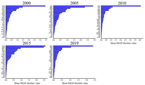
Figure 4.
The relative importance of PM2.5 concentrations influencing factors based on the mean absolute SHAP values for each of the selected years.
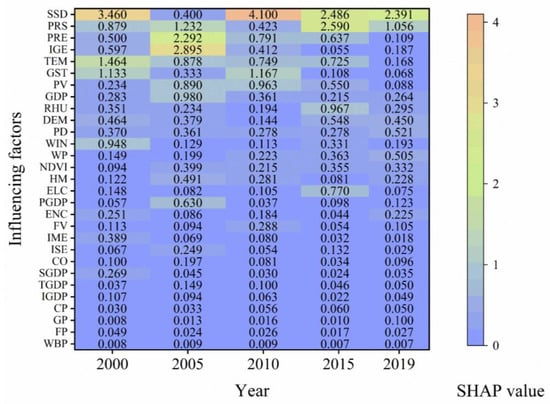
Figure 5.
Changes in SHAP values of influencing factors for the five selected years.
Table 3.
Importance ratio of influencing factors.
The SHAP algorithm differs from the way in which importance is estimated in the random forest method, as it not only uses absolute values but also computes density scatter plots to further analyze the direction and degree of influence of potential factors on PM2.5 concentrations. This is illustrated in Figure 6, whereby the x-axis designates SHAP values (positive or negative) for the various factors, while the y-axis indicates the level of contribution of input variables collected from selected locations, and the color denotes the feature value from low (blue) to high (red). Since SHAP values contain all the samples’ contributions in different locations, all influencing factors have a range of both positive and negative effects. The method, therefore, also illustrates the strength of the linear relationship between the selected influencing factors and PM2.5. For example, for GDP, whose importance ranked fourth in 2005, nearly half of the locations with high true values have a positive relation with PM2.5, while those with low values showed a negative impact.
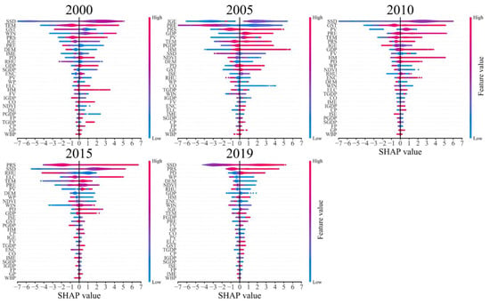
Figure 6.
The positive and negative impact of SHAP values in five selected years. Negative SHAP value means that the influencing factor at this location has a negative impact on PM2.5, and vice versa.
Partial dependence plots of the variables reveal their marginal effect on the predicted outcome of random forest outcomes. In this study, the plots reveal the direction and strength of influence of the various factors on PM2.5, as shown in Figure 7 and Supplementary Figures S1–S3. Across all five years, there is generally a negative correlation between PM2.5 concentrations and topography and land cover factors, including DEM and NDVI (Figure S2a,b), the significance of which decreases as the factor value increases, while the opposite is the case for the socioeconomic variables (Figure S3). There are, however, more complex patterns of correlation evidence in the meteorological variables. For example, PM2.5 is positively correlated with SSD when values are relatively small, but this shifts to a negative correlation at higher values (Figure S1b).
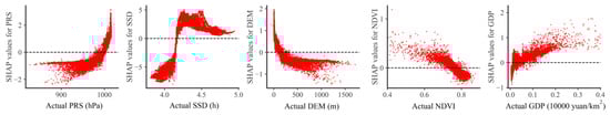
Figure 7.
Dependence plot of SHAP values of key influencing factors in 2000.
3.3. Spatial Variation of Influencing Factors Based on SHAP Values
Spatial variations in the SHAP values of influencing factors can be mapped in order to understand the relative contribution of these variables on PM2.5 in different regions of Zhejiang Province as described below for groups of factors associated with meteorological conditions, land surface conditions, and socioeconomic variables for the five sample years.
3.3.1. Meteorological Factors
Figure 8a illustrates the spatial distribution of SHAP values for PRS and suggests that aerosol pollution was more positively influenced by this factor in the plains and basins, especially around Hangzhou, Taizhou, and Wenzhou, while values in the mountainous areas were less strongly positive during the study period. Areas with higher atmospheric pressure, such as in the Hangjiahu and coastal plains, appear to be associated with elevated PM2.5 concentrations. Under such conditions, the regional transmission of aerosols is likely to be blocked, resulting in locally elevated values of PM2.5 [4,54]. Meanwhile, lower atmospheric pressures, as occur in upland areas of the province, appear to constrain PM2.5 concentrations [17]. Mountainous areas in the northwest, southwest, and central parts of Zhejiang province, which are windier in general, are characterized by reduced PM2.5 concentrations [18,55].
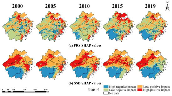
Figure 8.
Spatiotemporal variations in SHAP values for meteorological factors.
The effect (positive/negative) of SSD on PM2.5, which emerges in this study as one of the most influential factors, also varies between regions. For southwest mountainous areas, lower temperatures weaken the photochemical reaction and impede the formation of PM2.5 [56,57,58]. Central and western regions of the province, as well as the urban area around Hangzhou, exhibit the highest level of positive influence on aerosol concentrations, but the influence in the southwest mountainous areas is much lower (Figure 8b). More industrialized centers, including Hangzhou, Jinhua, and Quzhou, also associated with high temperatures and long sunshine duration, promote photochemical reactions and produce more precursors of PM2.5 and other secondary pollutants, thereby resulting in elevated PM2.5 concentrations [17]. The northern plains have the longest sunshine duration but lower surface temperatures, resulting in reduced accumulation of PM2.5, and therefore exhibit a weaker positive impact on PM2.5 [15]. This explains the observation, referred to in the previous sections, whereby SSD is positively correlated with PM2.5 at lower values, but this reverses at higher SSD values (Figure S1b).
3.3.2. Topography and Land Cover Factors
PM2.5 concentrations are shown to be closely correlated with DEM as values are higher at lower elevations (Figure S2a). Higher altitudes, especially in the southwestern part of the province, appear to suppress aerosol concentrations as higher wind speeds disperse PM2.5 [19]. On the other hand, low-lying areas, such as the northern and coastal plains and central basins, have a highly positive influence on PM2.5 (Figure 9a).
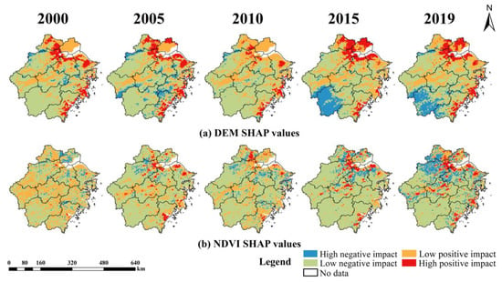
Figure 9.
Spatiotemporal variations in SHAP values for topography and land cover factors.
As shown in Figure S2b, NDVI has a significantly negative impact on PM2.5. Areas exhibiting the most strongly positive influence of NDVI are located in the major cities, while suburban and mountainous areas are associated with a negative effect (Figure 9b). In recent years, in regions with relatively high populations, including Hangzhou, Ningbo, and Wenzhou, the proportions of construction land and farmland have increased, thereby suppressing the typically negative effect of vegetation on PM2.5. In the hilly areas of Lishui and western Hangzhou, higher vegetation coverage has promoted the absorption and deposition of PM2.5, explaining the reduction in PM2.5 [30,59]. From 2005 onwards, the Zhejiang Province Government introduced woodland conservation measures [60], and this is evident in the area of the negative impact of NDVI expanding over time, as shown in Figure 9b. Consequently, the impact intensity of NDVI on PM2.5 was increasing as the negatively impacted area was significantly expanded.
3.3.3. Socioeconomic Factors
The concentration of PM2.5 in Zhejiang Province continued to decline from 2014 to 2018, which can be attributed to the introduction and implementation of a series of government policies, including the 2012 Zhejiang Province Air Pollution Prevention and Control Implementation Plan, the 2013 Zhejiang Province Air Pollution Prevention and Control Action Plan (2013–2017), and the 2014 Zhejiang Air Pollution Prevention and Control Action Plan Key Work Department Division Plan. Such policy measures appear to have had a marked impact on the relative influence of socioeconomic factors on air pollution, as suggested in this study and highlighted in the following analysis.
Generally, GDP and PM2.5 are positively correlated (Figure S3a), along with regions with higher GDP, especially in the cities (Figure 10a). The past few decades have been characterized by urbanizations and rapid economic development accompanied by increased energy consumption and exhaust emissions, therefore elevating PM2.5 concentrations [20,61]. In the less economically developed areas of the southwestern uplands, lower GDP values are associated with correspondingly low PM2.5 values. In 2000, before the economic boom, there were areas of very high positive impact (hotspots) in Hangzhou and Wenzhou, which expanded to all coastal cities as investment and consumption increased and led to higher levels of atmospheric pollution. During this time, the influence of GDP was continuously strengthening. However, from 2010 to 2019, even as GDP continued to increase, the relative importance of this factor was reduced, coinciding with the introduction of the air pollution control policies referred to above, together with the active adjustment of industrial structure in the province [62].

Figure 10.
Spatiotemporal variations in SHAP values for socioeconomic factors.
Population (PD) is, as expected, positively correlated with PM2.5 (Figure S3b). As shown in Figure 10b, the highly industrialized cities of Hangzhou and Wenzhou, in particular, were subject to rapid industrial agglomeration and increased production activities, thereby exhibiting increased pollutant emissions and energy consumption [63,64]. Dense housing and increased traffic aggravate PM2.5 pollution, further highlighting the positive effects of population on PM2.5 in cities [65]. However, in the more sparsely populated areas of the southwest mountains, PM2.5 values are correspondingly lower. The relatively stable SHAP values for PD suggest that it plays an important role in affecting the PM2.5 concentrations in Zhejiang Province, but as the structure of urban areas has been rationalized by more environmentally sensitive planning [66], the area of positive impact area has gradually reduced in 2019 (Figure 10b).
Changes in the characteristics of transportation associated with economic development have been substantial, for example, higher passenger volumes (PV), freight volumes, car ownership, and highway mileage, all of which increase fossil fuel consumption and road traffic emissions [30]. A positive correlation is evident between PV and PM2.5 (Figure S3c). Motor vehicle exhaust is one of the principal sources of PM2.5, discharging primary and secondary fine particles [27], exhibiting a positive impact on PM2.5. The area of Zhejiang with the strongest degree of influence of PV on pollution was, in 2010, situated mainly in the urban areas of Hangzhou, Jinqu Basin, and around the coast (Figure 10c). However, the degree of influence declined somewhat in 2019, possibly in response to the introduction of environmental policies. The provincial government has actively promoted lower carbon transport technologies, giving priority to public transport investment, constructing urban light rail systems, and favoring renewable energy vehicles [67]. For example, by 2016, more than 90% of the public buses in Hangzhou were powered by renewable energy. Compensated by the focus on sustainable urban transport, the increase in road networks and vehicles has not further augmented PM2.5 concentrations, and the SHAP values suggest that, in 2019, PV had little impact on PM2.5 (Figure 5).
The emission index, as anticipated, exhibits a positive effect on PM2.5 concentrations (Figure S3d), principally because fossil fuel combustion, construction dust, and secondary pollution contribute so much to PM2.5 [22]. Major industrial waste gas emissions (IGE) in the province include sulfur dioxide, nitrogen oxides, carbon dioxide, fluoride, soot, and productive dust. All these substances produced nitrates, sulfates, and secondary organic aerosols through atmospheric photochemical reactions, generating PM2.5 [68]. As Figure 10d shows, in 2005, IGE had the highest positive influence around the industrial cities of Quzhou, Hangzhou, and Taizhou. The introduction of air pollution control legislation from 2004, coupled with strengthened environmental supervision of air pollutant emitters, has promoted cleaner production and led to the elimination of outdated production systems and reduced the emission of volatile organic compounds from thermal power, steel, building materials, and other production processes. Meanwhile, the government has legislated for desulfurization and denitration in key industrial enterprises to prevent and control smoke and dust pollution [69]. In 2019, albeit with low SHAP values, IGE exhibits a positive impact on PM2.5 in most areas, indicating that the impact of the emission index had reduced, but energy conservation and emission reduction were still necessary. This evidence suggests that there is much potential in Zhejiang Province for further emission reduction and technological innovation as major targets for improving energy efficiency.
In terms of energy consumption, higher ELC is associated with increased PM2.5 concentrations (Figure S3e), especially when sourced from fossil fuels. Coal, which is a major source of pollutant precursors when combusted, is still the principal source of generating electricity, where the coal input for thermal power generation accounts for more than 70% of total power generation input in Zhejiang Province (China Energy Statistical Yearbook 2020). Figure 10e shows that it is the main urban centers that are most positively influenced by ELC, but that this area has been reduced since 2010 as a result of the introduction of renewable energy technologies, including photovoltaics for solar power, hydropower, and both wind and tidal power generators. This trend has been particularly noticeable since 2016 as the provincial authorities vigorously promoted the application of solar power and encouraged the development of centralized composite photovoltaic energy systems [67].
4. Discussion
Current popular methods of analyzing the relative importance of factors driving dependent variables, such as ordinary least squares [70] and geographic detectors [71,72], only acquire statistical values describing their relative importance. Although the output from the random forest algorithm reveals the relative significance of various drivers, the method is not suited to displaying the degree of influence spatially [32]. In this study, we employed a combination of random forest and Shapley additive explanations to reveal the spatiotemporal dynamics of factors’ driving patterns of PM2.5 pollution in Zhejiang Province, emphasizing the direction, strength, and spatial heterogeneity of underlying factors.
Given that Zhejiang Province, as with much of the rest of China, has experienced rapid economic growth over the last 2 or 3 decades, a detailed understanding of the role of economic factors in relation to atmospheric pollution is especially useful. The global interpretability feature of SHAP explanations reveals that growth of GDP initially led to sharp increases in atmospheric pollution but that the influence of increasing GDP declined more recently, a trend that parallels the inverted U-shaped environmental Kuznets curve [73]. These results are consistent with studies of PM2.5 in other parts of China [74], and indeed the course of atmospheric pollution in general. Shapley explanations further reveal that, while the intensity of influence of GDP, PD, and IGE may have weakened in urban areas in the recent past, such socioeconomic factors still contribute to atmospheric pollution. The local interpretability feature of the SHAP method reveals the complexity of spatiotemporal trends and highlights that even when the total degree of importance of a factor declines, the spatial coverage of its influence may not change. For example, across the Zhejiang province as a whole, IGE has declined in importance, but it remains significant in and around the major urban centers. In short, the level of detail regarding factors that determine the magnitude and spatial distribution of aerosols is of great potential value in the development of policy and strategy for pollution control and regulation.
Meteorological factors are shown to have the greatest significance in respect to PM2.5 among all the factors studied but are, of course, largely beyond any possibility of direct control. However, detailed monitoring of these factors may be helpful in developing early warnings of pollution events [75]. It is, on the other hand, possible to manage at least some of the land cover factors. For example, the results suggest that an emphasis on conserving (or even enlarging) the area of natural vegetation cover is a means of reducing PM2.5 pollution [76]. Moreover, adjusting land-use configuration [77], especially in urban areas such as Hangzhou, Shaoxing, and Ningbo, and increasing the proportion of urban green space [78] are known to have moderating effects on atmospheric pollution. Specific measures such as vertical planting, urban wind tunnel design [61], and rational spatial planning of green belts [79] should be encouraged.
Among the factors affecting PM2.5, the importance of meteorological factors is remarkable. A previous study mentioned that the intensity of direct solar radiation reaching the earth’s surface under clear-sky conditions is attenuated by gases and aerosols [80]. As SSD is defined as the daily sunshine duration during which the direct solar irradiance is greater than the threshold value of 120 Wm−2, it can effectively reflect the change of AOD (PM2.5). However, it is still difficult to clearly explain the internal mechanism for all the meteorological factors based on spatial SHAP values. In the future, we will consider combining the Weather Research and Forecast (WRF) model to quantitatively explain the specific reasons for their important change. Furthermore, meteorological conditions are constantly changing even within a day; the adopted PM2.5 data and recalculated meteorological data here are annual, which may bring great uncertainty and complexity to the mechanism analysis. Therefore, higher resolution of the original dataset both in time and space could be collected for more accurate consequences. In addition, the interaction analysis of influencing factors should be put forward in future research.
5. Conclusions
Based on multi-source data, the influence of meteorology, topography, land cover, and socioeconomic factors on PM2.5 was investigated; random forest and SHAP methods were combined to reveal the importance and spatiotemporal variation of key factors affecting PM2.5 in Zhejiang Province from 2000 to 2019. The main conclusions are as follows:
- (1)
- Three categories of factors exhibit different variation characteristics: the contribution of meteorological factors initially increases, but it has declined in the recent past. Changes in the importance of anthropogenic impacts such as GDP and PV (Passenger Volume) are opposite to that of meteorological factors, while the importance of topography and land cover factors continues to rise. However, the selected factors are generally ranked in terms of importance as follows: meteorological factors > social-economic factors > topography and land cover factors.
- (2)
- The spatial visualization of the relative importance of influencing factors in five years reveals that the details of their spatial change should be appreciated. Although the SHAP value representing relative importance was declined, the impacted coverage was not diminished. For example, among the socioeconomic drivers, even though the importance of PV and IGE has declined, they are still positively correlated with PM2.5 across the whole province and remain important sources of atmospheric pollution, prompting the need for further control measures.
- (3)
- The SHAP method is helpful to spatiotemporal visualization of influencing factors on PM2.5, especially for its outstanding local interpretability. For instance, the spatial distribution of the contribution of NDVI demonstrates that its negative impacted coverage is increased over the mountain areas, whereas the highly positive contribution in cities is also enlarged. This indicates that when ecological management concerned vegetation is implemented for PM2.5 regulation, more attention should be paid to the corresponding urban areas. Therefore, maps of SHAP values could be considered for putting forward practical advice.
Supplementary Materials
The following are available online at https://www.mdpi.com/article/10.3390/rs13153011/s1, Figure S1: Dependence plot of SHAP values of meteorological factors in five periods. Figure S2: Dependence plot of SHAP values of topography and land cover factors in five periods. Figure S3: Dependence plot of SHAP values of socioeconomic factors in five periods.
Author Contributions
Conceptualization, C.W. and X.L. (Xuan Li); methodology, X.L. (Xuan Li); software, E.L.; validation, Y.H.; writing—original draft preparation, X.L. (Xuan Li); writing—review and editing, C.W., M.E.M., Z.Z. (Zhaoyang Zhang), X.L. (Xingwen Lin), Z.Z. (Zhenzhen Zhang), Y.C. and M.F.; funding acquisition, C.W. All authors have read and agreed to the published version of the manuscript.
Funding
This research was funded by the Natural Science Foundation of Zhejiang Province (NO. LQ19D010007).
Data Availability Statement
The data presented in this study are available on request from the corresponding author.
Acknowledgments
The authors are thankful to the Institute for the Chinese Academy of Sciences and the Environment of the Hong Kong University of Science and Technology for the acccess of all the dataset, and we would like to acknowledge the Python Development Team for the open-source package for the modeling analysis. The authors also thank Editor Vera Li and four anonymous reviewers for their constructive comments, suggestions and help in enhancing the manuscript.
Conflicts of Interest
All authors declare no conflict of interest.
References
- Chen, Y.; Fung, J.C.H.; Chen, D.; Shen, J.; Lu, X. Source and exposure apportionments of ambient PM2.5 under different synoptic patterns in the Pearl River Delta region. Chemosphere 2019, 236, 124266. [Google Scholar] [CrossRef]
- Zhou, Y.; Chang, F.-J.; Chang, L.-C.; Kao, I.-F.; Wang, Y.-S.; Kang, C.-C. Multi-output support vector machine for regional multi-step-ahead PM2.5 forecasting. Sci. Total Environ. 2019, 651, 230–240. [Google Scholar] [CrossRef]
- Han, J.; Wang, J.; Zhao, Y.; Wang, Q.; Zhang, B.; Li, H.; Zhai, J. Spatio-temporal variation of potential evapotranspiration and climatic drivers in the Jing-Jin-Ji region, North China. Agric. For. Meteorol. 2018, 256–257, 75–83. [Google Scholar] [CrossRef]
- Hsu, C.-H.; Cheng, F.-Y. Classification of weather patterns to study the influence of meteorological characteristics on PM2.5 concentrations in Yunlin County, Taiwan. Atmos. Environ. 2016, 144, 397–408. [Google Scholar] [CrossRef]
- Yang, S.; Wu, H.; Chen, J.; Lin, X.; Lu, T. Optimization of PM2.5 Estimation Using Landscape Pattern Information and Land Use Regression Model in Zhejiang, China. Atmosphere 2018, 9, 47. [Google Scholar] [CrossRef] [Green Version]
- Zhang, X.; Hu, H. Hu Combining Data from Multiple Sources to Evaluate Spatial Variations in the Economic Costs of PM2.5-Related Health Conditions in the Beijing–Tianjin–Hebei Region. Int. J. Environ. Res. Public Health 2019, 16, 3994. [Google Scholar] [CrossRef] [Green Version]
- Huang, F.; Pan, B.; Wu, J.; Chen, E.; Chen, L. Relationship between exposure to PM2.5 and lung cancer incidence and mortality: A meta-analysis. Oncotarget 2017, 8, 43322–43331. [Google Scholar] [CrossRef] [PubMed] [Green Version]
- Sahu, S.K.; Chen, L.; Liu, S.; Ding, D.; Xing, J. The impact of aerosol direct radiative effects on PM2.5-related health risk in Northern Hemisphere during 2013–2017. Chemosphere 2020, 254, 126832. [Google Scholar] [CrossRef]
- Cao, C.; Jiang, W.; Wang, B.; Fang, J.; Lang, J.; Tian, G.; Jiang, J.; Zhu, T.F. Inhalable Microorganisms in Beijing’s PM2.5 and PM10Pollutants during a Severe Smog Event. Environ. Sci. Technol. 2014, 48, 1499–1507. [Google Scholar] [CrossRef] [PubMed]
- Shaltout, A.A.; Hassan, S.K.; Alomairy, S.E.; Manousakas, M.; Karydas, A.; Eleftheriadis, K. Correlation between inorganic pollutants in the suspended particulate matter (SPM) and fine particulate matter (PM2.5) collected from industrial and residential areas in Greater Cairo, Egypt. Air Qual. Atmos. Health 2018, 12, 241–250. [Google Scholar] [CrossRef]
- Shi, C.N.; Yuan, R.M.; Wu, B.W.; Meng, Y.J.; Zhang, H.; Zhang, H.Q.; Gong, Z.Q. Meteorological conditions conducive to PM2.5 pollution in winter 2016/2017 in the Western Yangtze River Delta. China Sci. Total Environ. 2018, 642, 1221–1232. [Google Scholar] [CrossRef]
- Zhang, Z.; Wu, W.; Fan, M.; Tao, M.; Wei, J.; Jin, J.; Wang, Q. Validation of Himawari-8 aerosol optical depth retrievals over China. Atmos. Environ. 2019, 199, 32–44. [Google Scholar] [CrossRef]
- Xu, X.; Dong, D.; Wang, Y.; Wang, S. The Impacts of Different Air Pollutants on Domestic and Inbound Tourism in China. Int. J. Environ. Res. Public Health 2019, 16, 5127. [Google Scholar] [CrossRef] [Green Version]
- Chen, D.; Xie, X.; Zhou, Y.; Lang, J.; Xu, T.; Yang, N.; Zhao, Y.; Liu, X. Performance Evaluation of the WRF-Chem Model with Different Physical Parameterization Schemes during an Extremely High PM2.5 Pollution Episode in Beijing. Aerosol Air Qual. Res. 2017, 17, 262–277. [Google Scholar] [CrossRef] [Green Version]
- Xu, H.; Bechle, M.J.; Wang, M.; Szpiro, A.A.; Vedal, S.; Bai, Y.; Marshall, J.D. National PM2.5 and NO2 exposure models for China based on land use regression, satellite measurements, and universal kriging. Sci. Total Environ. 2019, 655, 423–433. [Google Scholar] [CrossRef] [PubMed] [Green Version]
- Wang, X.; Dickinson, R.E.; Su, L.; Zhou, C.; Wang, K. PM2.5 Pollution in China and How It Has Been Exacerbated by Terrain and Meteorological Conditions. Bull. Am. Meteorol. Soc. 2018, 99, 105–119. [Google Scholar] [CrossRef]
- Zhang, C.; Ni, Z.; Ni, L. Multifractal detrended cross-correlation analysis between PM2.5 and meteorological factors. Phys. A Stat. Mech. Appl. 2015, 438, 114–123. [Google Scholar] [CrossRef]
- You, T.; Wu, R.; Huang, G.; Fan, G. Regional meteorological patterns for heavy pollution events in Beijing. J. Meteorol. Res. 2017, 31, 597–611. [Google Scholar] [CrossRef]
- Luo, J.; Du, P.; Samat, A.; Xia, J.; Che, M.; Xue, Z. Spatiotemporal Pattern of PM2.5 Concentrations in Mainland China and Analysis of Its Influencing Factors using Geographically Weighted Regression. Sci. Rep. 2017, 7, 40607. [Google Scholar] [CrossRef]
- Hao, Y.; Liu, Y.-M. The influential factors of urban PM2.5 concentrations in China: A spatial econometric analysis. J. Clean. Prod. 2016, 112, 1443–1453. [Google Scholar] [CrossRef]
- Yun, G.; Zuo, S.; Dai, S.; Song, X.; Xu, C.; Liao, Y.; Zhao, P.; Chang, W.; Chen, Q.; Li, Y.; et al. Individual and Interactive Influences of Anthropogenic and Ecological Factors on Forest PM2.5 Concentrations at an Urban Scale. Remote Sens. 2018, 10, 521. [Google Scholar] [CrossRef] [Green Version]
- Zou, Q.; Shi, J. The heterogeneous effect of socioeconomic driving factors on PM2.5 in China’s 30 province-level administrative regions: Evidence from Bayesian hierarchical spatial quantile regression. Environ. Pollut. 2020, 264, 114690. [Google Scholar] [CrossRef] [PubMed]
- Leung, D.M.; Tai, A.P.K.; Mickley, L.J.; Moch, J.M.; Van Donkelaar, A.; Shen, L.; Martin, R.V. Synoptic meteorological modes of variability for fine particulate matter (PM2.5) air quality in major metropolitan regions of China. Atmos. Chem. Phys. Discuss. 2018, 18, 6733–6748. [Google Scholar] [CrossRef] [Green Version]
- Chen, S.; Guo, J.; Song, L.; Li, J.; Liu, L.; Cohen, J.B. Inter-annual variation of the spring haze pollution over the North China Plain: Roles of atmospheric circulation and sea surface temperature. Int. J. Clim. 2019, 39, 783–798. [Google Scholar] [CrossRef]
- Yang, Q.; Yuan, Q.; Li, T.; Shen, H.; Zhang, L. The Relationships between PM2.5 and Meteorological Factors in China: Seasonal and Regional Variations. Int. J. Environ. Res. Public Health 2017, 14, 1510. [Google Scholar] [CrossRef] [Green Version]
- Chen, Z.; Chen, D.; Zhao, C.; Kwan, M.-P.; Cai, J.; Zhuang, Y.; Zhao, B.; Wang, X.; Chen, B.; Yang, J.; et al. Influence of meteorological conditions on PM2.5 concentrations across China: A review of methodology and mechanism. Environ. Int. 2020, 139, 105558. [Google Scholar] [CrossRef] [PubMed]
- Zhang, N.; Huang, H.; Duan, X.; Zhao, J.; Su, B. Quantitative association analysis between PM2.5 concentration and factors on industry, energy, agriculture, and transportation. Sci. Rep. 2018, 8, 9461. [Google Scholar] [CrossRef] [PubMed]
- Zhou, C.; Chen, J.; Wang, S. Examining the effects of socioeconomic development on fine particulate matter (PM2.5) in China’s cities using spatial regression and the geographical detector technique. Sci. Total Environ. 2018, 619, 436–445. [Google Scholar] [CrossRef]
- Wu, T.; Zhou, L.; Jiang, G.; Meadows, M.; Zhang, J.; Pu, L.; Wu, C.; Xie, X. Modelling Spatial Heterogeneity in the Effects of Natural and Socioeconomic Factors, and Their Interactions, on Atmospheric PM2.5 Concentrations in China from 2000–2015. Remote Sens. 2021, 13, 2152. [Google Scholar] [CrossRef]
- Yang, Q.; Yuan, Q.; Yue, L.; Li, T. Investigation of the spatially varying relationships of PM2.5 with meteorology, topography, and emissions over China in 2015 by using modified geographically weighted regression. Environ. Pollut. 2020, 262, 114257. [Google Scholar] [CrossRef]
- Naes, T.; Mevik, B.-H. Understanding the collinearity problem in regression and discriminant analysis. J. Chemom. 2001, 15, 413–426. [Google Scholar] [CrossRef]
- Zhang, Q.; Gao, W.; Su, S.; Weng, M.; Cai, Z. Biophysical and socioeconomic determinants of tea expansion: Apportioning their relative importance for sustainable land use policy. Land Use Policy 2017, 68, 438–447. [Google Scholar] [CrossRef]
- Chen, G.; Li, S.; Knibbs, L.D.; Hamm, N.A.S.; Cao, W.; Li, T.; Guo, J.; Ren, H.; Abramson, M.J.; Guo, Y. A machine learning method to estimate PM2.5 concentrations across China with remote sensing, meteorological and land use information. Sci. Total Environ. 2018, 636, 52–60. [Google Scholar] [CrossRef]
- Mangalathu, S.; Hwang, S.-H.; Jeon, J.-S. Failure mode and effects analysis of RC members based on machine-learning-based SHapley Additive exPlanations (SHAP) approach. Eng. Struct. 2020, 219, 110927. [Google Scholar] [CrossRef]
- García, M.V.; Aznarte, J.L. Shapley additive explanations for NO2 forecasting. Ecol. Inform. 2020, 56, 101039. [Google Scholar] [CrossRef]
- Gong, K.; Li, L.; Li, J.; Qin, M.; Wang, X.; Ying, Q.; Liao, H.; Guo, S.; Hu, M.; Zhang, Y.; et al. Quantifying the impacts of inter-city transport on air quality in the Yangtze River Delta urban agglomeration, China: Implications for regional cooperative controls of PM2.5 and O3. Sci. Total Environ. 2021, 779, 146619. [Google Scholar] [CrossRef] [PubMed]
- Wang, C.; Li, W.; Sun, M.; Wang, Y.; Wang, S. Exploring the formulation of ecological management policies by quantifying interregional primary ecosystem service flows in Yangtze River Delta region, China. J. Environ. Manag. 2021, 284, 112042. [Google Scholar] [CrossRef] [PubMed]
- Lou, W.; Wu, L.; Mao, Y.; Sun, K. Precipitation and temperature trends and dryness/wetness pattern during 1971–2015 in Zhejiang Province, southeastern China. Theor. Appl. Clim. 2018, 133, 47–57. [Google Scholar] [CrossRef]
- Wu, H.; Yang, C.; Chen, J.; Yang, S.; Lu, T.; Lin, X. Effects of Green space landscape patterns on particulate matter in Zhejiang Province, China. Atmos. Pollut. Res. 2018, 9, 923–933. [Google Scholar] [CrossRef]
- Wang, M.; Wang, H. Spatial Distribution Patterns and Influencing Factors of PM2.5 Pollution in the Yangtze River Delta: Empirical Analysis Based on a GWR Model. Asia-Pac. J. Atmos. Sci. 2021, 57, 63–75. [Google Scholar] [CrossRef]
- Wang, X.; He, S.; Chen, S.; Zhang, Y.; Wang, A.; Luo, J.; Ye, X.; Mo, Z.; Wu, L.; Xu, P.; et al. Spatiotemporal Characteristics and Health Risk Assessment of Heavy Metals in PM2.5 in Zhejiang Province. Int. J. Environ. Res. Public Health 2018, 15, 583. [Google Scholar] [CrossRef] [PubMed] [Green Version]
- Van Donkelaar, A.; Martin, R.; Brauer, M.; Boys, B.L. Use of Satellite Observations for Long-Term Exposure Assessment of Global Concentrations of Fine Particulate Matter. Environ. Health Perspect. 2015, 123, 135–143. [Google Scholar] [CrossRef] [PubMed] [Green Version]
- Lu, X.; Lin, C.; Li, W.; Chen, Y.; Huang, Y.; Fung, J.C.; Lau, A.K. Analysis of the adverse health effects of PM2.5 from 2001 to 2017 in China and the role of urbanization in aggravating the health burden. Sci. Total Environ. 2019, 652, 683–695. [Google Scholar] [CrossRef] [PubMed]
- Keller, W.; Borkowski, A. Thin plate spline interpolation. J. Geod. 2019, 93, 1251–1269. [Google Scholar] [CrossRef]
- Breiman, L. Random Forests. Mach Learn. 2001, 45, 5–32. [Google Scholar] [CrossRef] [Green Version]
- Johansson, U.; Boström, H.; Löfström, T.; Linusson, H. Regression conformal prediction with random forests. Mach Learn. 2014, 97, 155–176. [Google Scholar] [CrossRef] [Green Version]
- Strobl, C.; Boulesteix, A.-L.; Kneib, T.; Augustin, T.; Zeileis, A. Conditional variable importance for random forests. BMC Bioinform. 2008, 9, 307. [Google Scholar] [CrossRef] [Green Version]
- Rodriguez, J.D.; Perez, A.; Lozano, J.A. Sensitivity analysis of kappa-fold cross validation in prediction error estimation. IEEE Trans. Pattern Anal. Mach. Intell. 2010, 32, 569–575. [Google Scholar] [CrossRef]
- Xie, X.; Wu, T.; Zhu, M.; Jiang, G.; Xu, Y.; Wang, X.; Pu, L. Comparison of random forest and multiple linear regression models for estimation of soil extracellular enzyme activities in agricultural reclaimed coastal saline land. Ecol. Indic. 2021, 120, 106925. [Google Scholar] [CrossRef]
- Lundberg, S.M.; Lee, S.-I. A unified approach to interpreting model predictions. In Proceedings of the Advances in Neural Information Processing Systems, Long Beach, CA, USA, 4–9 December 2017; pp. 4765–4774. [Google Scholar]
- Padarian, J.; McBratney, A.B.; Minasny, B. Game theory interpretation of digital soil mapping convolutional neural networks. SOIL 2020, 6, 389–397. [Google Scholar] [CrossRef]
- Stirnberg, R.; Cermak, J.; Kotthaus, S.; Haeffelin, M.; Andersen, H.; Fuchs, J.; Kim, M.; Petit, J.-E.; Favez, O. Meteorology-driven variability of air pollution (PM1) revealed with explainable machine learning. Atmos. Chem. Phys. Discuss. 2021, 21, 3919–3948. [Google Scholar] [CrossRef]
- Chen, L.; Yao, X.; Liu, Y.; Zhu, Y.; Chen, W.; Zhao, X.; Chi, T. Measuring Impacts of Urban Environmental Elements on Housing Prices Based on Multisource Data—A Case Study of Shanghai, China. ISPRS Int. J. Geo-Inf. 2020, 9, 106. [Google Scholar] [CrossRef] [Green Version]
- Miao, Y.; Guo, J.; Liu, S.; Liu, H.; Zhang, G.; Yan, Y.; He, J. Relay transport of aerosols to Beijing-Tianjin-Hebei region by multi-scale atmospheric circulations. Atmos. Environ. 2017, 165, 35–45. [Google Scholar] [CrossRef]
- Jian, L.; Zhao, Y.; Zhu, Y.-P.; Zhang, M.-B.; Bertolatti, D. An application of ARIMA model to predict submicron particle concentrations from meteorological factors at a busy roadside in Hangzhou, China. Sci. Total Environ. 2012, 426, 336–345. [Google Scholar] [CrossRef]
- Chuang, M.-T.; Chou, C.C.-K.; Lin, N.-H.; Takami, A.; Hsiao, T.-C.; Lin, T.-H.; Fu, J.; Pani, S.K.; Lu, Y.-R.; Yang, T.-Y. A Simulation Study on PM2.5 Sources and Meteorological Characteristics at the Northern tip of Taiwan in the Early Stage of the Asian Haze Period. Aerosol Air Qual. Res. 2017, 17, 3166–3178. [Google Scholar] [CrossRef] [Green Version]
- Liu, C.-N.; Lin, S.-F.; Tsai, C.-J.; Wu, Y.-C.; Chen, C.-F. Theoretical model for the evaporation loss of PM2.5 during filter sampling. Atmos. Environ. 2015, 109, 79–86. [Google Scholar] [CrossRef]
- Yang, X.; Zhao, C.; Guo, J.; Wang, Y. Intensification of aerosol pollution associated with its feedback with surface solar radiation and winds in Beijing. J. Geophys. Res. Atmos. 2016, 121, 4093–4099. [Google Scholar] [CrossRef]
- Wu, W.; Zhang, M.; Ding, Y. Exploring the effect of economic and environment factors on PM2.5 concentration: A case study of the Beijing-Tianjin-Hebei region. J. Environ. Manag. 2020, 268, 110703. [Google Scholar] [CrossRef] [PubMed]
- Xiong, B.; Chen, R.; Xia, Z.; Ye, C.; Anker, Y. Large-scale deforestation of mountainous areas during the 21 st Century in Zhejiang Province. Land Degrad. Dev. 2020, 31, 1761–1774. [Google Scholar] [CrossRef]
- Liu, X.-J.; Xia, S.-Y.; Yang, Y.; Wu, J.-F.; Zhou, Y.-N.; Ren, Y.-W. Spatiotemporal dynamics and impacts of socioeconomic and natural conditions on PM2.5 in the Yangtze River Economic Belt. Environ. Pollut. 2020, 263, 114569. [Google Scholar] [CrossRef] [PubMed]
- Ma, Z.; Liu, R.; Liu, Y.; Bi, J. Effects of air pollution control policies on PM2.5 pollution improvement in China from 2005 to 2017: A satellite-based perspective. Atmos. Chem. Phys. Discuss. 2019, 19, 6861–6877. [Google Scholar] [CrossRef] [Green Version]
- Chen, L.; Wei, Q.; Fu, Q.; Feng, D. Spatiotemporal Evolution Analysis of Habitat Quality under High-Speed Urbanization: A Case Study of Urban Core Area of China Lin-Gang Free Trade Zone (2002–2019). Land 2021, 10, 167. [Google Scholar] [CrossRef]
- Lou, C.-R.; Liu, H.-Y.; Li, Y.-F. Socioeconomic Drivers of PM2.5 in the Accumulation Phase of Air Pollution Episodes in the Yangtze River Delta of China. Int. J. Environ. Res. Public Health 2016, 13, 928. [Google Scholar] [CrossRef] [PubMed] [Green Version]
- Yun, G.; He, Y.; Jiang, Y.; Dou, P.; Dai, S. PM2.5 Spatiotemporal Evolution and Drivers in the Yangtze River Delta between 2005 and 2015. Atmosphere 2019, 10, 55. [Google Scholar] [CrossRef] [Green Version]
- Xu, P.; Jin, P.; Yang, Y.; Wang, Q. Evaluating Urbanization and Spatial-Temporal Pattern Using the DMSP/OLS Nighttime Light Data: A Case Study in Zhejiang Province. Math. Probl. Eng. 2016, 2016, 9850890. [Google Scholar] [CrossRef] [Green Version]
- Wang, K.; Yan, M.; Wang, Y.; Chang, C.-P. The impact of environmental policy stringency on air quality. Atmos. Environ. 2020, 231, 117522. [Google Scholar] [CrossRef]
- Wang, P.; Cao, J.; Tie, X.; Wang, G.; Li, G.; Hu, T.; Huang, R.-J.; Zhan, C.; Wu, Y.; Xu, Y.; et al. Impact of Meteorological Parameters and Gaseous Pollutants on PM2.5 and PM10 Mass Concentrations during 2010 in Xi’an, China. Aerosol Air Qual. Res. 2015, 15, 1844–1854. [Google Scholar] [CrossRef] [Green Version]
- Zhang, Q.; Zheng, Y.; Tong, D.; Shao, M.; Wang, S.; Zhang, Y.; Xu, X.; Wang, J.; He, H.; Liu, W.; et al. Drivers of improved PM2.5 air quality in China from 2013 to 2017. Proc. Natl. Acad. Sci. USA 2019, 116, 24463–24469. [Google Scholar] [CrossRef] [Green Version]
- Zhao, X.; Zhou, W.; Han, L.; Locke, D. Spatiotemporal variation in PM2.5 concentrations and their relationship with socioeconomic factors in China’s major cities. Environ. Int. 2019, 133, 105145. [Google Scholar] [CrossRef] [PubMed]
- Yang, D.; Wang, X.; Xu, J.; Xu, C.; Lu, D.; Ye, C.; Wang, Z.; Bai, L. Quantifying the influence of natural and socioeconomic factors and their interactive impact on PM2.5 pollution in China. Environ. Pollut. 2018, 241, 475–483. [Google Scholar] [CrossRef]
- Zhou, L.; Zhou, C.; Yang, F.; Che, L.; Wang, B.; Sun, D. Spatio-temporal evolution and the influencing factors of PM2.5 in China between 2000 and 2015. J. Geogr. Sci. 2019, 29, 253–270. [Google Scholar] [CrossRef] [Green Version]
- Bilgili, F.; Nathaniel, S.P.; Kuşkaya, S.; Kassouri, Y. Environmental pollution and energy research and development: An Environmental Kuznets Curve model through quantile simulation approach. Environ. Sci. Pollut. Res. 2021, 1–16. [Google Scholar] [CrossRef]
- Ding, Y.; Zhang, M.; Chen, S.; Wang, W.; Nie, R. The environmental Kuznets curve for PM2.5 pollution in Beijing-Tianjin-Hebei region of China: A spatial panel data approach. J. Clean. Prod. 2019, 220, 984–994. [Google Scholar] [CrossRef]
- Song, Y.; Qin, S.; Qu, J.; Liu, F. The forecasting research of early warning systems for atmospheric pollutants: A case in Yangtze River Delta region. Atmos. Environ. 2015, 118, 58–69. [Google Scholar] [CrossRef]
- Lu, D.; Xu, J.; Yue, W.; Mao, W.; Yang, D.; Wang, J. Response of PM2.5 pollution to land use in China. J. Clean. Prod. 2020, 244, 118741. [Google Scholar] [CrossRef]
- Ouyang, X.; Wei, X.; Li, Y.; Wang, X.-C.; Klemeš, J.J. Impacts of urban land morphology on PM2.5 concentration in the urban agglomerations of China. J. Environ. Manag. 2021, 283, 112000. [Google Scholar] [CrossRef]
- Lei, Y.; Davies, G.M.; Jin, H.; Tian, G.; Kim, G. Scale-dependent effects of urban greenspace on particulate matter air pollution. Urban For. Urban Green. 2021, 61, 127089. [Google Scholar] [CrossRef]
- Guo, L.; Luo, J.; Yuan, M.; Huang, Y.; Shen, H.; Li, T. The influence of urban planning factors on PM2.5 pollution exposure and implications: A case study in China based on remote sensing, LBS, and GIS data. Sci. Total Environ. 2019, 659, 1585–1596. [Google Scholar] [CrossRef]
- Li, J.; Liu, R.; Liu, S.C.; Wang, J.; Zhang, Y.; Shiu, C.-J. Trends in aerosol optical depth in northern China retrieved from sunshine duration data. Geophys. Res. Lett. 2016, 43, 431–439. [Google Scholar] [CrossRef] [Green Version]
Publisher’s Note: MDPI stays neutral with regard to jurisdictional claims in published maps and institutional affiliations. |
© 2021 by the authors. Licensee MDPI, Basel, Switzerland. This article is an open access article distributed under the terms and conditions of the Creative Commons Attribution (CC BY) license (https://creativecommons.org/licenses/by/4.0/).