Abstract
Floating LIDAR systems (FLS) are a cost-effective way of surveying the wind energy potential of an offshore area. However, as turbulence intensity estimates are strongly affected by wave-induced buoy motion, it is essential to correct them. In this study, we quantify the turbulence intensity measurement error of a WindCube v2® mounted on a 12-ton anchored buoy as a function of met-ocean conditions, and we construct a subsequently applied correction method suitable for 10-min wind LIDAR data storage. To this end, we build a model to simulate the effect of buoyancy movements on the LIDAR’s wind measurements. We first apply the model to understand the mechanisms responsible for the wind LIDAR measurement error. The effect of the buoy’s rotational and translational motions on the radial wind speed measurements of the individual beams is first studied. Second, the temporality induced by the LIDAR operation is taken into account; the effect of motion subsampling and the interaction between the different measurement beam positions. From this model, a correction method is developed and successfully applied to a 13-week experimental campaign conducted off the shores of Fécamp (Normandie, France) involving the buoy-mounted WindCube v2® compared with cup anemometers from a met mast and a fixed WindCube v2® on a platform. The correction improves the linear regression against the fixed LIDAR turbulence intensity measurements, shifting the offset from ~0.03 to ~0.005 without post-processing the remaining peaks.
1. Introduction
Wind power has been a growing source of energy worldwide for the past 30 years. As the atmospheric boundary layer conditions vary drastically depending on the location on the planet, prospecting a geographical location for the development of a wind farm requires a thorough understanding of the wind behavior over the course of several years to determine its optimal size and economic potential [1]. Atmospheric turbulence is an extremely important factor in this assessment. It induces fluctuations in the loads applied to the wind turbine blades, which lead to structural fatigue and a potential decrease in aerodynamic performance [2]. The standard instrument for atmospheric boundary layer wind measurements is a combination of anemometers and wind vanes installed at different altitudes on a meteorological mast (met mast). The cost of mast installation and maintenance is very high, especially for offshore applications. A cheaper alternative is the use of wind LIDARs (LIght Detection And Ranging) to perform atmospheric boundary layer wind measurements from the ground.
In this study, we essentially focus on profiler wind LIDARs. A profiler wind LIDAR measures radial wind speeds at different positions and altitudes using the Doppler effect and calculates the vertical wind speed profile. Wind LIDARs have been used in many onshore [3,4,5] and offshore [6,7,8] studies for decades. The 10-min mean wind velocity estimate of a commercial continuous-wave (CW) or pulsed profiler wind LIDAR is generally as accurate as that provided by cup or sonic anemometers [9]. However, wind LIDARs are not an established technology for accurately measuring atmospheric turbulence. Both CW and pulsed profiler LIDARs show a significant measurement bias, compared to the reference instruments [10], which depends on boundary layer stability and measurement altitude. The main errors induced by profiler technology are: Spatial averaging due to the large measurement volume [11], cross-contamination between the different components of the velocity vector [12,13] and low temporal sampling rate of the measurement [14]. Despite these systematic biases, profiler wind LIDARs are very practical devices because of their ease of installation and relocation, and their ability to provide a reasonable estimation of atmospheric boundary layer behavior in a wide range of applications. In offshore applications, a large part of the planet is hardly accessible for fixed platforms due to the extreme depth of the oceans and the required financial investment for the deployment of this type of installation. A wind LIDAR mounted on a buoy is a commercially viable tool for investigating the atmospheric behavior in oceanic areas. We refer to this set-up as floating LIDAR system (FLS).
The sea-induced motion of a FLS is highly dependent on the dynamic response of the buoy to wave behavior. The shape, weight and anchorage of the buoy have a significant influence on the motion experienced by the wind LIDAR. The buoy’s motion has six degrees of freedom: Three are translational (surge, sway, heave) and three are rotational (roll, pitch, yaw). The six degrees of wave-induced motion of the buoy each affect the LIDAR Doppler measurements in their own way. Generally, wave motion introduces a bias of the order of 1–2% in the measurement of the 10-min averaged velocity vector by a profiler FLS [15]. In contrast, the turbulence intensity measurement is heavily impacted by sea motion, whether it be pulsed or CW technology [16,17]. Wave-induced buoy motion tends to add variability to the Doppler measurements. Therefore, a 10-min turbulence intensity estimate from the floating LIDAR is generally overestimated compared to the reference measurement. The bias between the FLS and anemometer measurements depends on the sea conditions and the dynamic response of the buoy to the waves and can be up to several times the anemometer measurement. The FLS measurements can be corrected by associating the wind LIDAR with an Inertial Measurement Unit (IMU) measuring the movements of the buoy at high frequency. One correction method involves processing each of the radial wind speed measurements according to the IMU to cancel the effect of the buoy’s motion. A detailed review of this method is presented in [16]. This method is based on a strong interaction between the two devices for a real-time correction, or on a storage of all the time series from the LIDAR and the IMU for a subsequently applied correction.
In this study, we focus on the pulsed profiler WindCube v2® LIDAR from Leosphere®. The contribution of this paper consists in a less computationally intensive model-based correction estimating the atmospheric turbulence from the time series of an IMU and the 10-min statistics of a pulsed floating LIDAR. By grouping the corrections of each radial measurement of the LIDAR in global matrices, this method reduces the need for time synchronization between the two devices and reduces the amount of data to be stored. The use of a simple model also allows to study and understand the influence of the buoy’s movements on the floating wind LIDAR measurement. In Section 2, we explain the theory from the WindCube v2® LIDAR as well as the contribution of an IMU for buoy motion measurement. In Section 3, we present the model and its implementation for estimating the atmospheric turbulence intensity from 10-min floating LIDAR statistics. Then, we present the experimental conditions from the campaign conducted off the shores of Fécamp (Normandie, France), and its measurements were used to evaluate the correction method. In Section 4, we apply the model to understand buoyancy motions of increasing complexity; from the effect of a sinusoidal motion with one degree of freedom on a single measurement radius to the motions of the experimental validation campaign.
2. LIDAR Theory
LIDAR technology is used in various operational contexts, which are adapted to the desired measurement. For the measurement of the wind resource in the atmospheric boundary layer, two categories are distinguished: Pulsed and Continuous-Wave (CW) LIDARs [18]. Both technologies are coherent LIDARs measuring the speed of particles within the atmosphere using the Doppler effect. The principle of coherent LIDARs is to mix the radiation backscattered by the particles, considered as passive tracers, with that of the local reference beam in order to reliably calculate the frequency of the backscattered signal with a light beating process and finally, to deduce the wind speed at a given position [9]. In this study, we focus on the pulsed LIDAR technology and more specifically on the profiler LIDAR designed by Leosphere®: WindCube v2®.
2.1. WindCube Coordinate System and Calculated Quantities
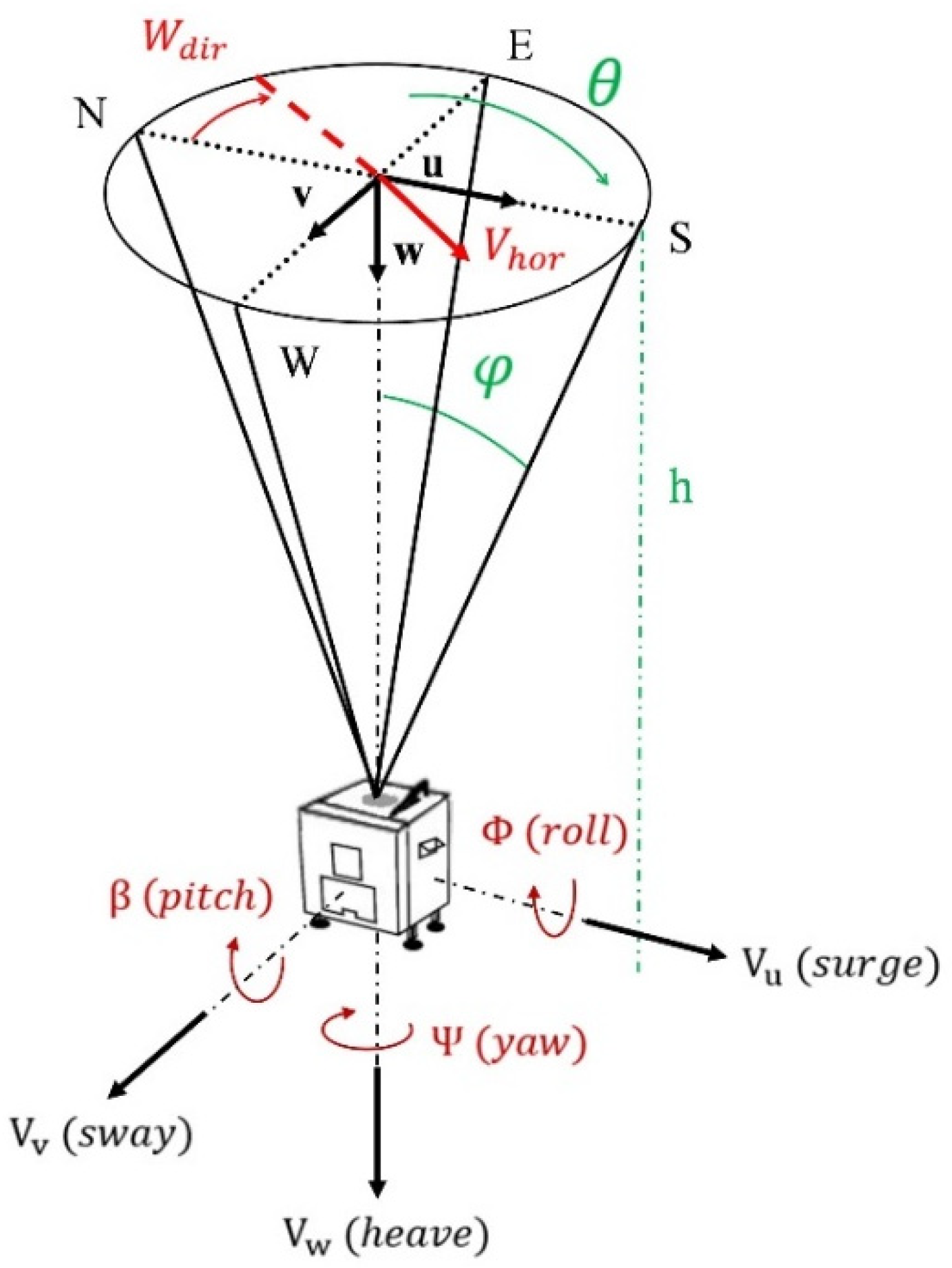
The WindCube v2® emits laser pulses into five fixed directions, four inclined at and one vertical. The directions are defined by the angles and , respectively the azimuth angle measured clockwise from the north of the LIDAR, and the elevation angle measured from the zenith position (Figure 1) In the LIDAR reference frame, the angles defining the five line-of-sight (LOS) directions are (in degrees): and .

Figure 1.
WindCube v2® pulsed LIDAR principle and the six degrees of freedom of buoy-induced motion.
The LOS radial wind speed measurements from the five beam directions are combined to define the wind vector at several altitudes as:
We note that the components , and of the wind vector are specified in the coordinate system defined in the LIDAR reference frame and are not referred to an absolute coordinate system. At each altitude, the horizontal wind speed and direction are deduced from the wind vector :
with being the offset between the LIDAR north and the magnetic North. The turbulence intensity () is calculated from the statistical study of horizontal wind speed measurements:
The coordinate system is defined by the direction of the beams (Figure 1). The x-component is oriented from N to S, the y-component is oriented from E to W and the z-component points towards the ground at the zenith position.
2.2. WindCube Principle
2.2.1. Line-of-Sight Radial Wind Speed Measurement
The five laser directions of the WindCube v2® are maintained for a duration of 0.8 s for the non-vertical beams and 1 s for the vertical position. During a LOS measurement, repeated laser pulses are sent from the LIDAR to the particles in the atmospheric boundary layer. As the time of light propagation is the unit used to evaluate the distance from the LIDAR to the particle backscattering the laser, the duration of the laser pulse induces an uncertainty in the position of the particle within the probe volume [19]. In the case of the WindCube, the pulses have a duration of 175 ns. Therefore, for each pulse, the backscattered signal is temporally sliced into range gates and a weighting function is applied to each of the sliced signals to take into account the filtering effect exerted by the probe volume on the measured radial wind speed [14]. At the end of a LOS measurement, a mean radial wind speed and a carrier to noise ratio (CNR) are determined at several altitudes using the maximum likelihood estimator (MLE) method to the averaged spectrum of all the pulses [20].
2.2.2. Doppler Beam Swinging (DBS) Principle
Each laser direction is defined by the angles et , and the normalized vector pointing from the LIDAR towards the particles is defined by:
The LOS radial wind speed measurements are defined for each beam direction in the opposite sens of the vector, as a function of the wind vector at the given altitude . They are geometrically characterized by:
The measured at each fixed positions are combined to determine the wind speed vector at the altitude :
Therefore, DBS LIDARs combine radial wind speed measurements made at different positions and times to derive a velocity vector. Two main measurement errors are introduced by this principle: The filtering of smaller scales due to the large size of the probe volume [14], and the two-point correlation contamination between the wind field components, known as variance contamination or cross-contamination [10].
2.3. Floating LIDAR Systems (FLS)
In the case of a buoy mounted LIDAR (FLS), the motion induced by the dynamic response of the buoy to waves affects the wind LIDAR measurement. As the LIDAR principle is defined for a stationary position, a motion-induced variation in the velocity measurement contaminates the FLS measurements. The measurement contamination arises from two causes: the instantaneous tilt of the LIDAR due to roll, pitch and yaw angles, and the translational movement of the platform modifying the perceived velocity at the measurement point [21]. In order to quantify the effect of motion on the wind LIDAR measurement, it is essential to measure the movement of the buoy using an Inertial Measurement Unit (IMU). The IMU measures the translational and rotational motion of the buoy in the three axes using accelerators and gyroscopes, providing six degrees of freedom of motion. The orientation of the motion frame used in this study is shown in Figure 1.
Roll, pitch and yaw measurements () from the IMU can be used to correct the direction of the floating LIDAR’s measurement beams. The rotation matrix allows to turn the rotated LIDAR reference frame into a non-rotated reference frame [21]. It is defined by:
The rotation into the non-rotated reference frame is applied to a wind vector measured in the LIDAR reference frame by a dot product with the rotation matrix . The use of the IMU’s rotational and translational measurements allows the physics of the buoy’s motion, induced by its geometry, weight and anchorage, to be taken into account in constructing a correction to the motion-induced wind measurement contamination. The use of an IMU for FLS measurements correction requires two conditions. The first is the alignment of the coordinate systems from the IMU and the wind LIDAR, a re-alignment can be performed in case of an offset [20]. The second is an equivalent position of the two devices relative to the center of gravity of the buoy, this induced error can also be corrected [21]. In this study, the two devices are aligned and close enough not to need these corrections.
3. Method
3.1. A Model-Based Method for Correcting the 10-min TI Measurements from the Wind LIDAR
The variance of a floating LIDAR horizontal wind speed measurement has two main sources. The first is the natural variance induced by the turbulent structures encountered in the atmospheric boundary layer (), the one we seek to assess. The second is the variance induced by the motion of the LIDAR in its six degrees of freedom (), the one we estimate using the model. The theory of the method is based on the hypothesis that, at a given average wind speed, wave-induced motion and atmospheric turbulence are independent events.
Therefore, according to the properties of independent variables, we can decompose the variance of the FLS uncorrected measurements () into:
The atmospheric turbulence intensity can be deduced from the standard deviation calculated by the model:
For the purpose of estimating , the model simulates the operation of a WindCube v2® in a turbulence-free (or constant) atmospheric wind for a measurement period of 10 min. The model requires the temporal data from an IMU and the 10-min statistics of the floating LIDAR measurements (mean horizontal wind speed, mean wind direction, mean vertical wind speed). The considered velocity vector is the 10-min average wind measurement from the floating LIDAR, it is defined for each altitude by:
with , and the 10-min means of the three wind components. The model is based on an incremental temporal discretization. At each time step, the IMU measurements are interpolated and the theoretical measurement from the evaluated beam subjected to the motion is calculated. At the end of a line-of-sight measurement, the evaluated measurements are averaged to deduce the theoretical LOS wind speed measurement. At the end of the evaluated 10-min period, the 10-min statistics from the model provide the variance induced by the motion of the LIDAR. The model principle for calculating the theoretical radial wind speed measurement in a given direction is explained in details in Section 3.1.1 and the method for estimating the 10-min motion-induced variance is detailed in Section 3.1.2.
We define the horizontal velocity variance estimator for n LOS measurements during the 10 min as follows:
with the horizontal velocity (Equation (2)) and the time corresponding to the end of the LOS measurements.
We note that the variance formulation is referred to as an estimator as the samples are not uniformly distributed over time, as the LOS measurement time is not constant.
In this study, we define the measurement time for each of the WindCube v2® LOS directions as , as estimated from the experimental measurement files. By default, the LOS direction at t=0 is the north axis of the LIDAR reference frame. After its LOS measurement time, the orientation of the beam moves according to the vector . The choice of the first beam orientation has a strong impact on the 10-min wind statistics, its influence is studied in detail in Section 4.2.3. The time step of the model needs to be small enough to consider all the effects induced by the motion on the LIDAR measurements, but not too large to keep a low computational cost. We define the temporal discretization at 10 Hz.
3.1.1. Measurement from One Line-of-Sight Subjected to Wave-Induced Motion
The radial wind speed measured by a line-of-sight from a moving LIDAR is impacted by two major phenomena: The alteration of the measurement cone geometry induced by the rotational angles, and the influence of the translational velocity. At time , the local roll , pitch and yaw angles as well as the surge , sway and heave translational velocities are estimated by linear interpolation of the IMU measurements. The effect of beam angular velocity is not considered here as it is applied in the beam direction’s normal plane, so it has little or no influence on the measurement.
We also note that the tilt of the LIDAR implies a change in the measurement altitude in addition to the change in the geometry of the measurement cone. The two phenomena have opposite effects: Increasing the tilt angle tends to decrease the measurement altitude and thus to encounter lower wind speeds because of wind shear, but the decrease in the angle relative to the horizontal wind tends to increase the radial wind speed measurement. In this study, we did not include this effect in the model. However, its influence is expected to be quite small. Kelberlau et al. [16] estimated from their offshore dataset the factor by which the effect of changed scanning geometry is reduced by the effect of wind shear.
We first study the effect of the alteration of the measurement cone geometry. At time , the LIDAR measurement cone is defined by the angles and for each beam direction. In order to estimate the effect of the geometric transformation, we need to calculate the actual angles (in the non-rotated reference frame) of the laser beam at each discretized time in the model. We apply the rotation () to the non-rotated normalized vector defined for each direction (Equation (5)), through the rotation matrix (Equation (8)):
Then, we calculate the angles and from the rotated vector :
with and being respectively the first and second component of the rotated normalized beam vector. Finally, according to Equation (6), the radial wind speed theoretically measured by the beam at position at time is calculated by:
During a line-of-sight measurement in a given direction (approximate time 1 s), there is sufficient time for the roll, pitch and yaw angles to vary significantly (Figure 3). The set of discrete points contained in the time of a LOS measurement are combined and averaged to estimate the overall effect of the geometry change. Therefore, for a LOS measurement at position of duration performed between times and , the average radial wind speed including the effect of the geometry modification of the measurement cone is calculated by:
with the times and being evaluated by the model and the time step of the model for a 10 Hz time discretization.
Now, we study the effect of the translational velocities of the buoy, affecting the radial wind speed measurements from the LIDAR. They are considered as added velocities to the atmospheric wind speed in the definition of the radial wind speed in Equation (6). At time , the translational velocity vector () is constructed from the surge , sway , and heave measurements by the IMU in the rotated frame of the buoy. It is then projected onto the normalized vector of the beam position oriented towards the LIDAR, as is the LIDAR measurement vector. Therefore, the radial velocity induced by the translational motion of the LIDAR () is calculated by:
The effect of translational velocity during a LOS measurement is calculated by associating and averaging the discrete points within its duration. Thus, for a LOS measurement at position of duration performed between times and , the mean influence of the translational velocity of the LIDAR on the radial velocity is calculated by:
3.1.2. Estimated Motion-Induced Variance for 10 min of FLS Measurement
The laser beam of the WindCube v2® measures only one position at a time. It uses the average radial velocities previously measured at the other positions to calculate the velocity vector at the end of a LOS measurement (Equation (7)). Therefore, at a time subsequent to the times corresponding to the end of the line-of-sight measurements in the directions , the three components of the wind speed vector are calculated at altitude by:
We note that the effect of translational velocity on the measured LIDAR velocity is subtracted from the wind measurement because, if the two phenomena are oriented in the same direction, the translational velocity tends to absorb a part of the atmospheric wind speed.
With the variance estimator defined in Equation (12), we can directly calculate the motion-induced variance using a matrix system. It is first necessary to carry out the development of the equations of and Equations (A1) and (A2) in Appendix A). Then, thanks to the distributive nature of multiplication with respect to addition and to the constant wind speed at altitude , we identified:
with being the component of the vector .
Therefore, the influences of rotational and translational motions on the LIDAR turbulence intensity measurement are stored in the 10-min averaged matrices: , , , , , , and . All these matrices can be calculated using the model and the time series from the IMU without the knowledge of the mean velocity vector measured by the LIDAR.
The horizontal velocity calculation within the model, however, requires the knowledge of the 10-min mean velocity vector. It is affected by the assumptions of the model and must take into account all the physics involved. Therefore, we cannot safely estimate it with the mean horizontal velocity measured by the FLS. The calculation of the variance being based on a quadratic sum, a small error in the value of the horizontal velocity can have strong consequences on the estimated variance. The discrepancy in value between the mean velocity measured by the FLS and the one evaluated by the model is mainly due to three model hypotheses: The boundary layer shear not taken into account, the default initial direction of the beam and the LOS measurement time of each beam considered constant.
Therefore, the horizontal velocity is calculated within the model according to:
with and developed in Appendix A. If a user wants to subsequently apply the correction to the 10-min turbulence intensity measurements, it is necessary to store the entire time series from IMU and the 10-min statistics from the floating LIDAR to run the model. Compared to a beam-by-beam correction, this method allows to store less information from the LIDAR measurements. The use of averaged matrices over 10 min also reduces the influence of an imperfect synchronization of the clocks of the two instruments. Moreover, the use of a model to estimate 10-min motion-induced turbulence reduces the impact of yaw measurement drift. However, our method is based on simplifying hypotheses, thus, the beam-by-beam correction remains the most theoretically precise, for more information on this type of correction, refer to [16].
3.2. Experimental Campaign
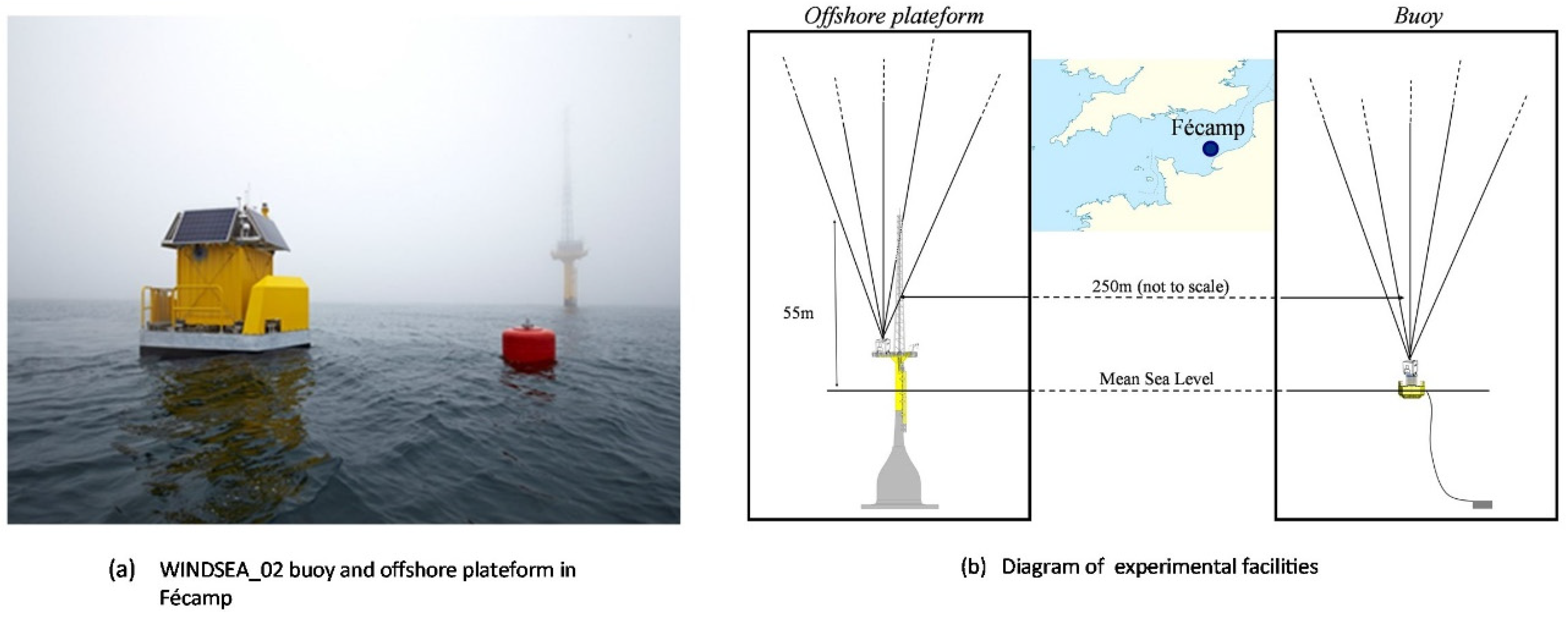
The correction developed for FLS turbulence intensity estimate is evaluated on experimental data from a floating WindCube v2®. The FLS measurements are compared with data measured by an anemometer and an additional WindCube v2® located on a fixed platform. The experimental campaign took place off the shores of Fécamp (Normandie, France) from 20 April 2018 to 31 October 2018 (6-month trial period). The test site is located at an approximate distance of 14 km from the coast. The distance between the measuring buoy and the platform is 250 m (Figure 2).

Figure 2.
Presentation of the experimental means deployed on the site 14 km off the coasts of Fécamp. (a) Photograph of the WINDSEA_02 buoy (in the foreground) accompanied by the wave buoy (in red). The fixed platform is visible in the background. (b) Diagram of the experimental means, the dimensions are not respected and the LIDAR is not to scale.
Both LIDARs allow measurements at 12 altitudes between 40 m and 200 m, plus the natural elevation due to the buoy (3.5 m to Mean Sea Level, MSL) or the platform (14.4 m to MSL). The measurement mast (erected by EDF Renouvelables®) is equipped with two anemometers (Risoe P2546 A horizontal boom-mounted) at altitudes 33.8 m and 54.8 m to MSL. Only the measurements from the cup anemometer located at altitude 54.8 m are used in this study. For all the results presented in Section 4.3, the data measured by a WindCube at the desired height for comparison with the anemometer are linearly interpolated from the twelve evaluated altitudes. In the comparisons of the floating LIDAR to the fixed LIDAR, since the fixed LIDAR is taken as the reference, we interpolate the floating LIDAR measurements to the altitudes evaluated by the fixed LIDAR.
The floating wind LIDAR is mounted on the WINDSEA_02 buoy developed by AKROCEAN® (France). The 12-ton buoy (Figure 2a) is powered by solar panels, a turbine in the wave tank, methanol cartridges and batteries. Through the wave tank, the system uses passive mechanical stabilization to limit the motion of the buoy. The buoy is anchored to the ground and the mooring line is connected to an intermediate buoy to limit the effect of line tension on the buoy movement. A wave buoy is associated with the WINDSEA_02, providing 30-min statistics of waves behavior (height and period). The WindCube v2® installed on the buoy is associated with an IMU measuring the six degrees of freedom () at a frequency rate of 10 Hz. We note that the dynamic behavior of the buoy in response to wave motion depends on its geometry, weight and anchorage. The IMU measurements are directly related to a particular buoy, and are not representative of all experimental setups. The use of inertial measurements to correct the wind LIDAR measurements captures all the physics of the buoy motion perceived by the wind LIDAR. We also note that the yaw measurements from an IMU tend to drift over time. In our study, the model used for the turbulence intensity correction relies on the relative temporal dynamics of the yaw motion in a 10-min interval. Since the drift occurs on time scales longer than 10 min, we keep the yaw measurement from the IMU unchanged.
For confidentiality reasons, not all six months of data could be processed. 13 weeks have been selected to reflect the range of meteorological conditions typically encountered by the floating LIDAR at this site. A K-means clustering method [22] was used to segregate the hourly datasets according to wind (mean wind, direction and boundary layer shear coefficient), wave (period and mean height) and atmospheric (temperature and precipitation height) conditions. Seven clusters emerged from the K-means method. Subsequently, the seven most representative weeks of the clusters and the six harshest weeks were selected to build the 13 weeks dataset. The wind data used for the clustering were measured by the floating LIDAR, the wave data by the wave buoy and the atmospheric data were extracted from the most representative point of the ERA5 mesh. The ERA5 mesh point is located at a distance equivalent to that of the FLS from the coast (about 15 km) and at a distance of 18 km from the Fécamp test site.
LIDAR data is filtered out of the 13 weeks by availability ( for a 10-min sample), wind speeds ( m/s and m/s) and turbulent intensities (). Assuming that the lattice mast has a small influence on the behavior of the atmospheric boundary layer at the evaluated altitudes (between 55 m and 200 m), we consider all wind directions. After the application of the filters, approximately 5200 samples of 10 min are considered, i.e., about 30 full days.
4. Results and Discussion
For a full understanding of the sea motion effect on a floating pulsed LIDAR, we proceed in a stepwise fashion. First, we estimate values of rotational angle and translational velocity representative of the experimental conditions of the WINDSEA_02 buoy at sea. Then, the effect of motions is studied on the theoretical horizontal velocity measurement using the model described in Section 3.1. Finally, the effect of wave induced motion on FLS measurement is studied on the Fécamp experimental campaign and the correction is applied to the floating WindCube v2® measurements.
4.1. IMU Measurements as a Function of Sea Conditions
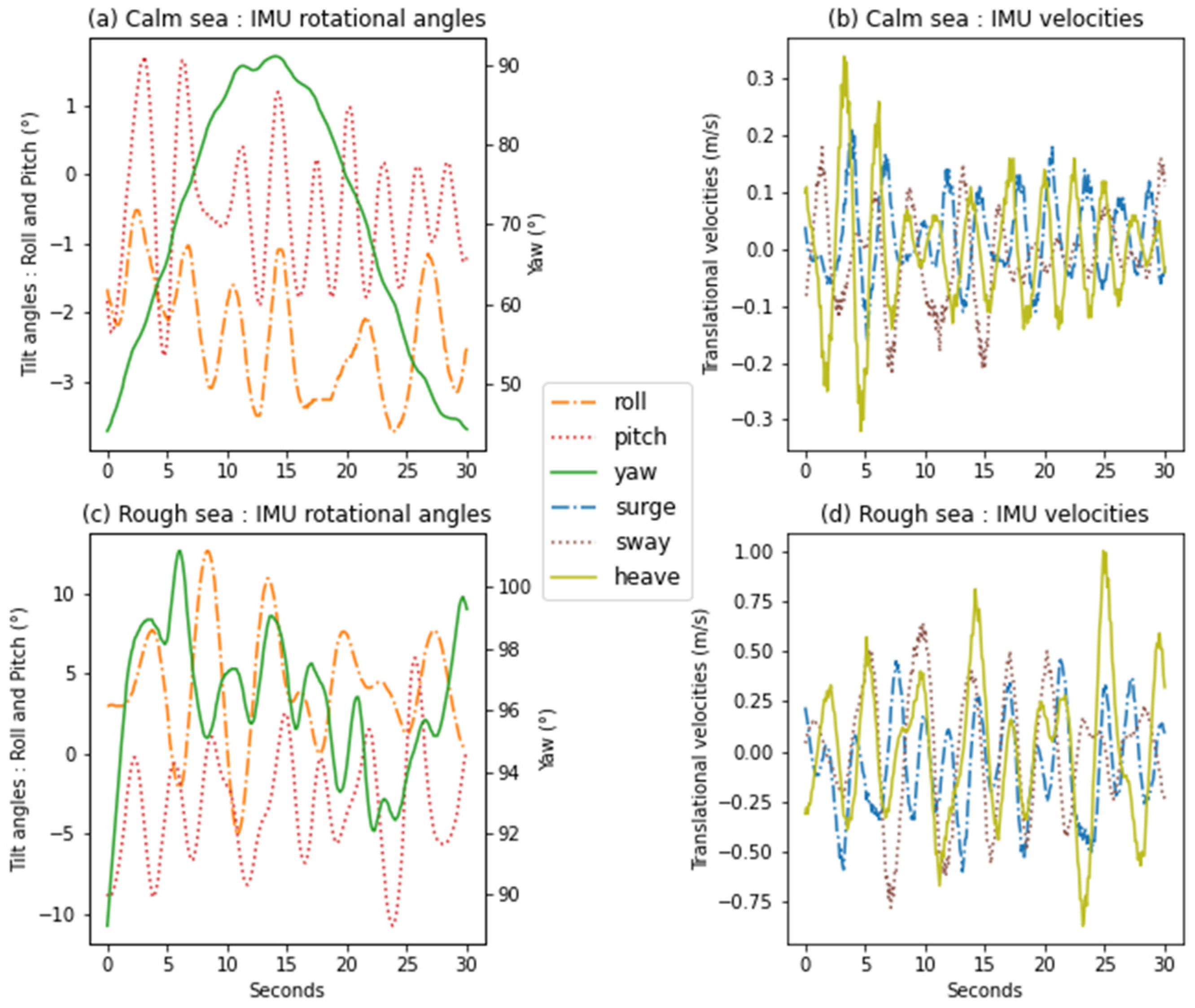
Through wave buoy data, sampled every 30 min, we identify two representative samples of calm and rough sea conditions to illustrate different aspects of the buoy’s motion. For observing the temporal evolution of the IMU data, we extract the last 30 s of the 30-min samples for visualization. The sea conditions are selected using the mean wave height and the mean period of all waves. As wave height and period are highly correlated (Figure 13b), calm conditions are represented by low values (, ) and rough conditions by high values (, ). The measurements of the six degrees of freedom of the inertial station on the picked 30-s samples are presented in the Figure 3.

Figure 3.
Measurements of the six degrees of freedom from the IMU on board of the WINDSEA_02 buoy. Rotational angles are presented for calm; and (a) rough; (c) sea conditions. Translational velocities are presented for calm; and (b) rough; (d) sea conditions.
We first discuss the rotational angle measurements (Figure 3a,c). In calm seas (a), the buoy performs a flapping motion introducing tilt movements (roll and pitch) with an amplitude of a few degrees and a period of the order of 4 to 5 s. At the same time, the buoy rotates, introducing yaw measurements with a high amplitude of about 30 degrees and a period of 30 s. In rough seas (c), the buoy’s flapping is intensified as the waves are more intense. The tilt motions (roll and pitch) exhibit an amplitude of 5 to 10 degrees with a period of about 4 to 5 s. The yaw behaves very differently in rough seas compared to calm seas, it is strongly affected by the waves and its evolution is similar to the tilt. Its amplitude is of the order of 10 degrees and its period of about 4 to 5 s.
For the translational velocity measurements (Figure 3b,d), in calm seas (b), the surge, sway and heave have a roughly similar amplitude of about 0.1 m/s. The period of the surge and sway is of the same order as the tilt flap, about 4 to 5 s. The heave has a shorter period because it reacts to every small change in sea surface height. In rough seas (d), the three translational degrees of freedom have a similar amplitude of the order of 0.5 m/s, we note that the heave tends to have larger peak values than the surge and sway. The periods of the translational velocities are still about 4 to 5 s.
We can now use these observations to estimate the theoretical error induced by a sinusoidal movement of the same magnitude. We note that these measurements are specific to the WINDSEA_02 buoy used in this study. Its dimensions, shape, anchorage and means of supply (turbine in the wave tank) have a strong impact on its dynamic behavior.
4.2. Theoretical Impact of Buoy Movements on the FLS Horizontal Velocity Estimates
The buoy motion influences the wind LIDAR velocity measurement in several ways. We separate three distinct effects; the effect of motion on the cone geometry and on the perceived relative velocity; the effect of subsampling due to the temporal averaging of several pulses in the same beam direction, and; the interaction effect between the different beam measurements.
In order to understand the influence of the various degrees of freedom of motion on the LIDAR measurement, we consider the case of a purely horizontal non-turbulent wind (). As the directions of the WindCube v2® measurement beams are symmetrical in the horizontal plane, roll and pitch have a similar effect on the beams having the same relative position to their rotation axis. Therefore, for the sake of simplicity, we combine these two motions and decompose the rotational motions into two effects: Tilt and yaw. The motions are represented by zero-centred sinusoids, defined by an amplitude and period , of the form:
For a gradual understanding, we first study the reaction of a single LIDAR beam measurement to a period of tilt and yaw. In a second step, we study the effect of the temporality of the measurements, including the effect of subsampling and the effect of interaction between the different beam directions. Based on the study of the order of magnitude of the IMU measurements, we consider the amplitudes: , ) and m/s.
4.2.1. Horizontal Velocity Bias from an Isolated LIDAR Beam Subjected to a Period of Rotation
The study of motion-induced radial wind speed variability of an isolated beam provides an understanding of the dynamic behavior of the LIDAR during a LOS measurement. It is the study of the geometric effect of motion on the velocity perceived by the wind LIDAR’s beams. The translational movements of the buoy appear as an added component to the velocity vector measured by the LIDAR. The consideration of this phenomenon on the LIDAR measurement is presented in the model formulation in Section 3.1.1. As the modification of the measurement cone geometry of the LIDAR has a less intuitive effect on the measurements, we focus here on the effect of the buoy’s rotations.
4.2.2. Tilt Motion
In this section, care has been taken to make all the results independent of the nature of the tilt (pitch or roll), so the directions of the rays are defined by A, B, C, D and Z for zenith. The effect of tilt on the angles and of the beams in the different directions of the WindCube v2® is studied in Figure 4. The horizontal velocity is decomposed into two components: component in the A–C beams plane and the component in the B–D beams plane.
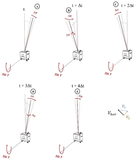
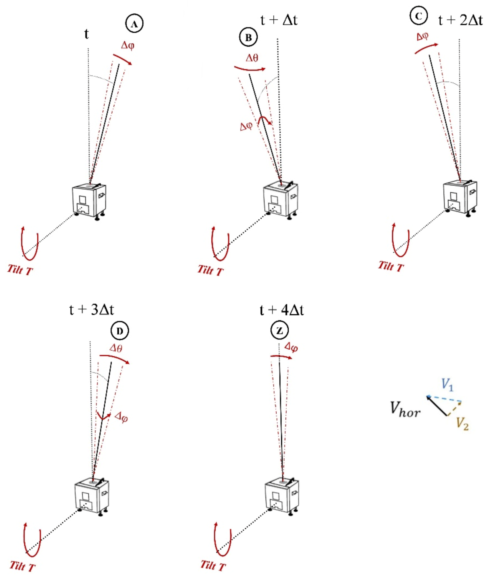
Figure 4.
Diagram representation showing the influence of a tilt change (roll or pitch) on the angles and of the five measurement directions of the WindCube v2® denoted A, B, C, D, Z (side view). The suggested times are added to recall the temporality of the WindCube measurement. The horizontal velocity is decomposed into two components: and .
For beams A and C, the tilt only affects the angle . And for beams B and D, the tilt modifies and . The effect on the measurements is a composition of two angular effects. In the Z case, the ray is at the zenith and the tilt has an effect only on φ. As the horizontal velocity measurement is only affected by the measurements of the beams A, B, C and D, we do not study here in detail the zenith beam.
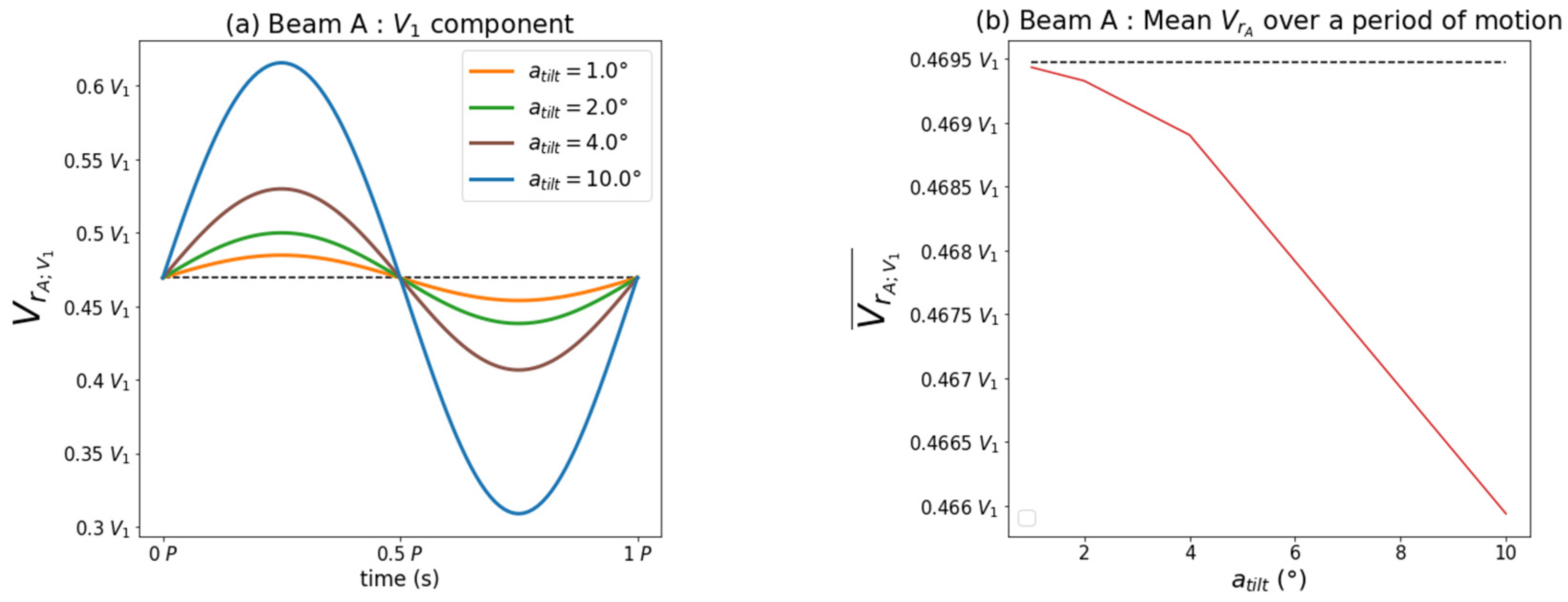
We first focus on the rays in the normal plane to the tilt axis (beams A–C). In this plane, only the angle is affected by the rotational movement, it evolves in a linear way with the tilt: . Therefore, only the component of the incident horizontal wind affects the radial wind speed measurement. We present here the effect of motion on the measurement of beam A. The radial wind speed is calculated according to the Equation (6):
The tilt of the LIDAR has the effect of increasing or decreasing the value of which directly affects the value of the measured readial velocity (Figure 5a). The larger the value of , the more aligned the beam is with the horizontal velocity and the greater the radial wind speed measurement. In Figure 5b, it is observed that this effect is not uniformly distributed around the value . The properties of the sine function around the angle bring more influence to the decrease of the angle than to its increase. Thus, the average measurement of the beam A is affected by the tilting motion. For an entire period of tilt of amplitude , the average measurement of the beam is decreased by less than 1%.

Figure 5.
Response of the beam A to a sinusoidal motion of tilt as a function of the incident wind component . (a) radial wind speed as a function of time relative to the period of the sinusoid. (b) Time-averaged value of the radial wind speed as a function of the sinusoid amplitude.
We note that the same tilting movement has an opposite effect on the radial wind speed measured by beam C. Thus, if the measurements were carried out simultaneously at both directions A and C, the tilting movement would have very little influence on the measurement of the velocity component by the WindCube v2®. However, in a real case, the measurements are not simultaneous and this effect has a strong influence on the LIDAR measurement.
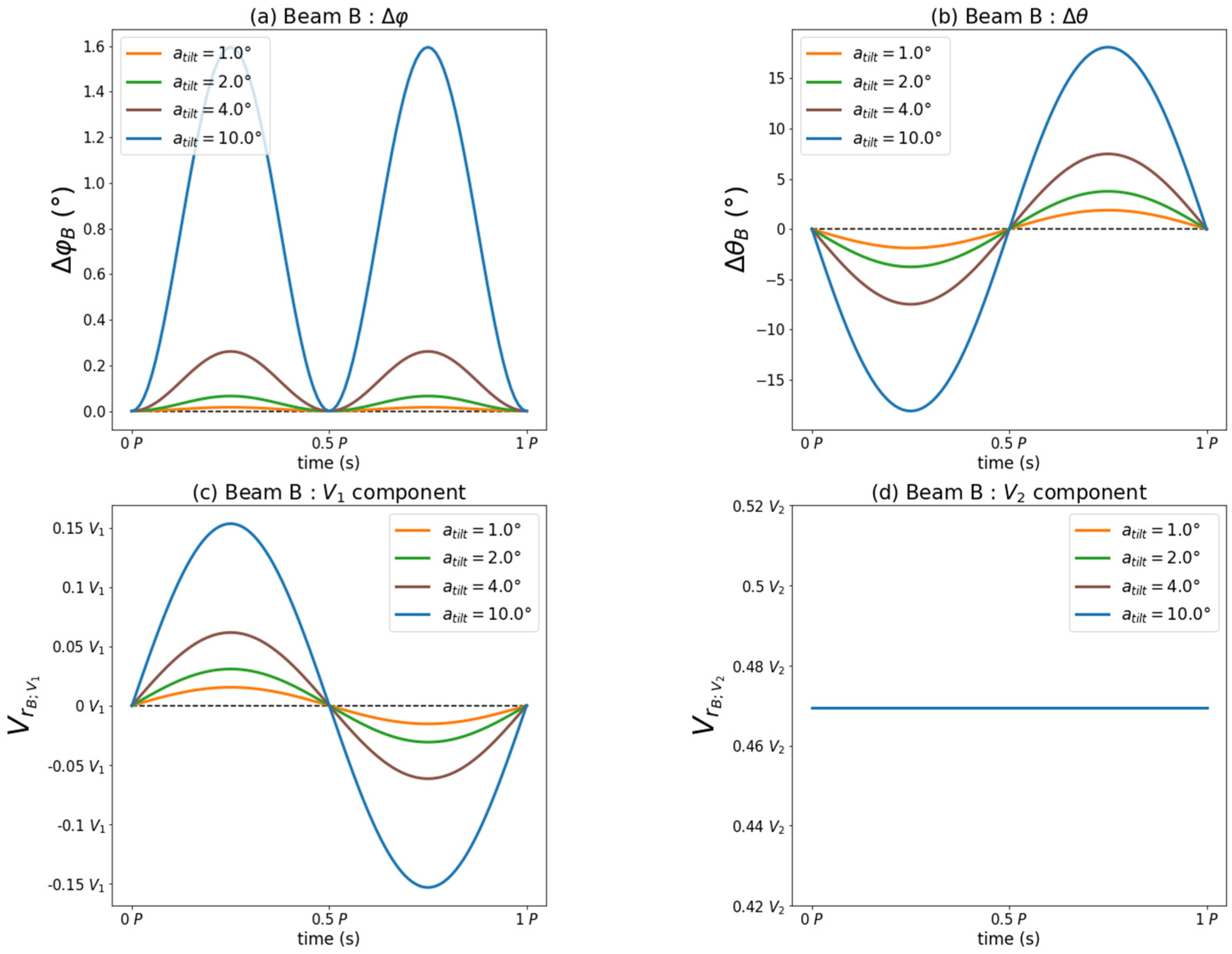
Now, we focus on the beams in the plane parallel to the tilt axis (beams B-D). In this plane, the motion simultaneously affects the angles and of the beams. Here, we present the effect of the tilt on the radial wind speed measurement from beam B. Figure 6a,b show the influence of a period of sinusoidal motion on the variation of angles and of beam B: and . The variation is defined as the difference of the angle subjected to the motion with respect to its original position. The angle evolves counterclockwise for a positive inclination. While the angle is accentuated whatever the sign of the tilt . Since the angles and are modified by the tilt, the measurements of the radius B are impacted by both wind components and :
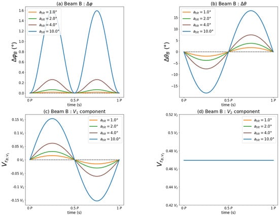
Figure 6.
Response of the beam B to a sinusoidal motion of tilt as a function of the incident wind components and . The results are plotted as a function of the time relative to the period of the sinusoid. (a) Motion-induced variation of the angle . (b) Motion-induced variation of the angle . (c) Variation of the component according to of the radial wind speed. (d) Variation of the component of the radial wind speed.
The measurement of the component of the radial wind speed is impacted by the tilt motion (Figure 6c). Since beam B is originally perpendicular to the wind component , it is not supposed to measure it. However, the tilt modifies and the measurement of beam B is impacted by the component. The measurement of the component is not affected by the tilt movement (Figure 6d). The effects induced by the simultaneous changes in the angles and compensate each other to remove this error.
We note that the same tilting movement has an equivalent effect on the radial wind speed measurement of beam D. If the measurements were made simultaneously at both directions B and D, the effects of the tilting movements on the two opposite beams would be additive.
We can now determine the dominant effect induced by tilting on the horizontal wind measurement. For a tilt along a given axis, only the component of the incident wind, perpendicular to the axis of rotation, has an influence on the measurement of the four non-vertical rays. We consider here the case of a whole period of sinusoidal motion of amplitude and we evaluate the order of magnitude of the influence of this motion on the measurement of the different rays. While the average measurement is barely affected by the tilting motion, a large amount of variability is introduced into the time series of the measurement. The effects on the rays parallel (beams B–D) and perpendicular (beams A–C) to the axis of rotation introduce an equivalent standard deviation on the radial wind speed measurement, of the order of . However, the influence on the horizontal velocity variation is not equivalent. In order to estimate this influence, let us assume an incident wind following the component () and a variation introduced by a tilt on the measurement of the wind component in the plane of each pair of rays. Considering , using a Reynolds decomposition and the Equation (2), we compare:
- The effect of a variation of in the measurement of the component measured by A-C rays:
- The effect of a variation of in the measurement of the component measured by B-D rays:
There is an order of magnitude of discrepancy between the two estimates: . In the case of an isolated tilt , the most influential effect on the horizontal wind measurement is the variation of the angle on the beams perpendicular to the rotation axis (beams A–C).
4.2.3. Yaw Movement
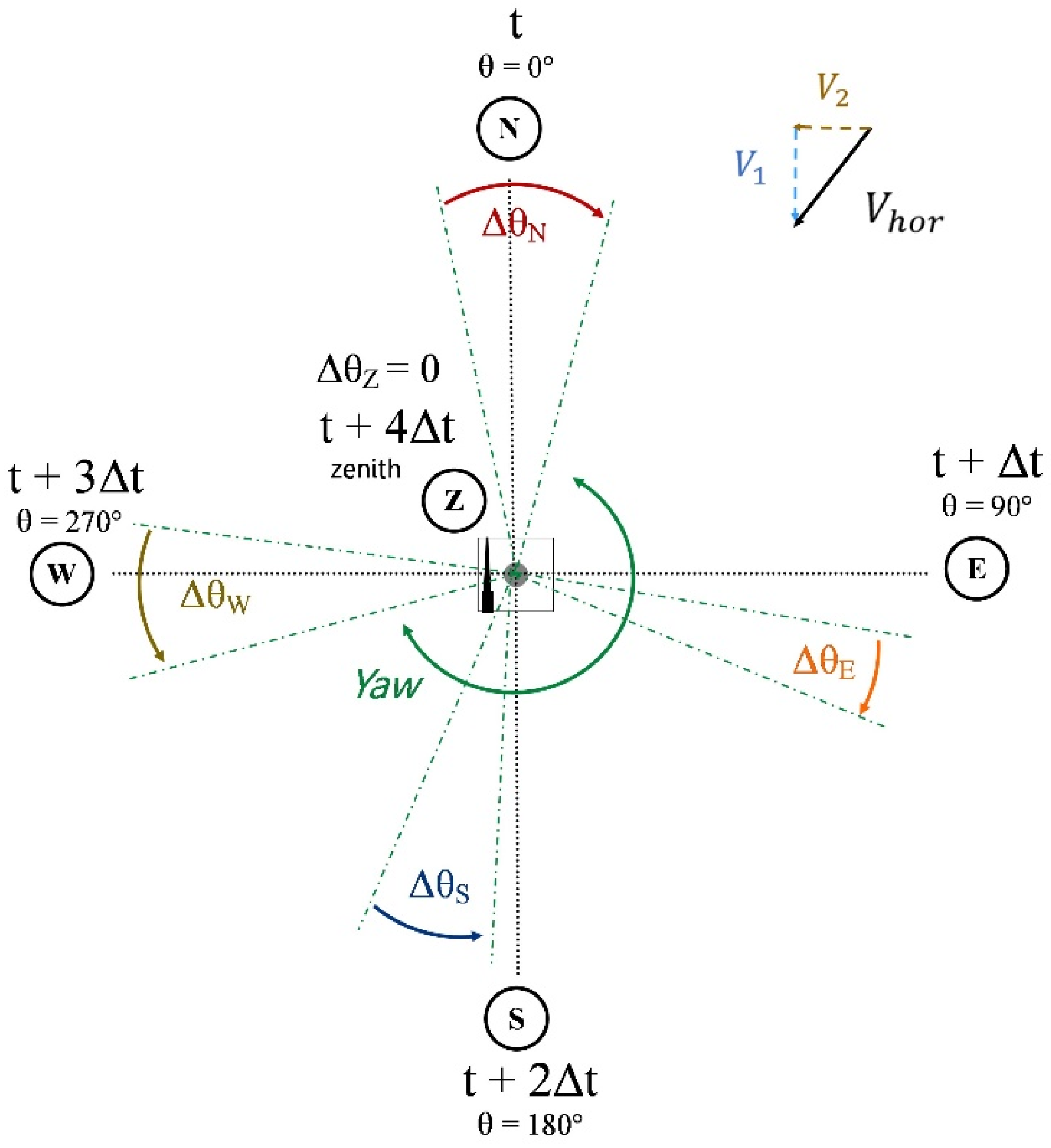
As yaw only has one degree of freedom, we relate to the rays here by their more common label: . The effect of yaw on the angle of the different WindCube rays v2 is studied in Figure 7. The horizontal velocity is decomposed into two components: the component in the N-S beams plane and the component in the E-W beams plane. and correspond to the and axes in the WindCube v2® reference frame (Figure 1).
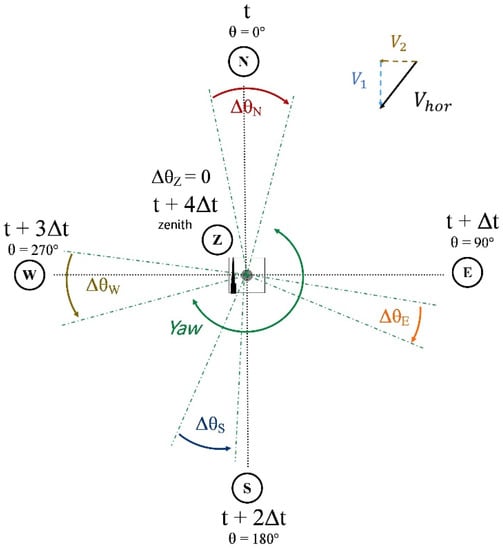
Figure 7.
Diagram representation showing the influence of a yaw variation on the angles of the five measurement directions of the WindCube v2® (top view). The suggested times are added to recall the temporality of the WindCube measurement. The horizontal velocity is decomposed into two components: and .
For the four non-vertical beams, yaw is in the same plane as the angle , so it is linearly affected by the rotation: . For the beam at the zenith, an isolated yaw motion has no effect on its geometry. However, it is important to bear in mind that yaw will affect the vertical measurement in the case of a tilted LIDAR.
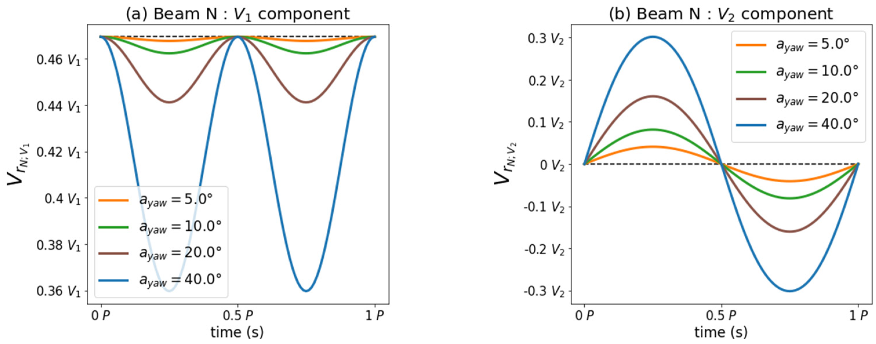
As the angles of the non-vertical rays are modified by yaw, the measurements of the four rays are impacted by the two wind components and . Here we present the effect of motion on the measurement of the N beam:
The ray N is originally aligned with the component of the incident wind (Figure 7). Thus, the radial wind speed measurement is decreased by the LIDAR motion regardless of the yaw direction (Figure 8a). The component depends on the direction of rotation because it depends on the orientation of the beam with respect to the component of the incident wind (Figure 8b).
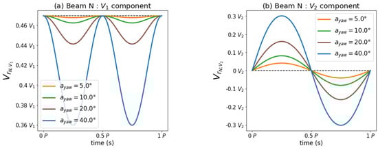
Figure 8.
Influence of a sinusoidal yaw motion on the radial wind speed measurement of the beam N as a function of the incident wind components and . All the results are plotted as a function of the amplitude of the motion and the time relative to the period of the sinusoid. (a) Variation of the component. (b) Variation of the component.
We note that, in the hypothetical case of a simultaneous measurement of all the rays, the effect of the yaw on the horizontal speeds measured by the four non-vertical rays would be cancelled and only the direction of the wind measured would be modified. However, in the real case, the influence of the yaw depends on the movement-measurement temporality and yaw motion affects the LIDAR’s horizontal speed measurements.
4.2.4. Effect of Motion Subsampling for an Isolated Beam
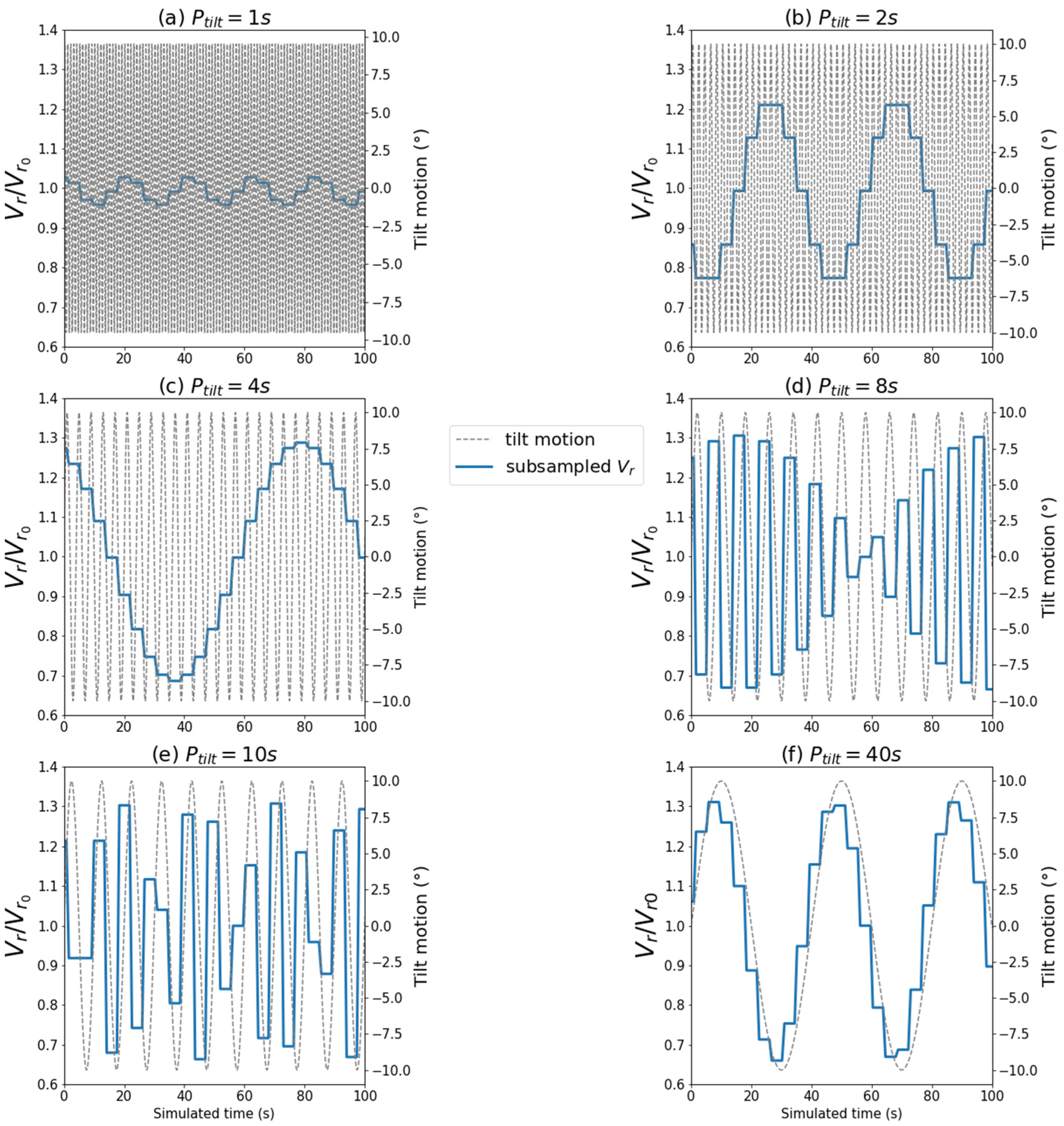
Now, we take into account the timing of the alternative measurements of the rays. We recall here that the approximate LOS measurement times of the five rays are defined by: . The measurement of a given beam occurs approximately every 4.2 s and for a duration of about 0.8 to 1 s. During a LOS measurement time, the six degrees of freedom of motion of the buoy shift. The radial wind speed measurement is an average of a large number of measurements subjected to different movements. In addition to this phenomenon, a motion subsampling effect is induced by the incremental evolution of the beam direction, which returns to its original position every 4.2 s. These phenomena apply to rotational (roll, pitch, yaw) and translational (surge, sway, heave) motions and can strongly influence the radial wind speed measurement of one line-of-sight. In order to observe the influence of subsampling on the measured radial wind speed, we consider the ray A described in Section 4.2.2, aligned to the component , subjected to a tilting motion of amplitude .
Figure 9 shows an example of subsampling and averaging on the radial wind speed measurement. The radial wind speed is calculated with Equation (24) and is normalized by the value measured in the motionless case .
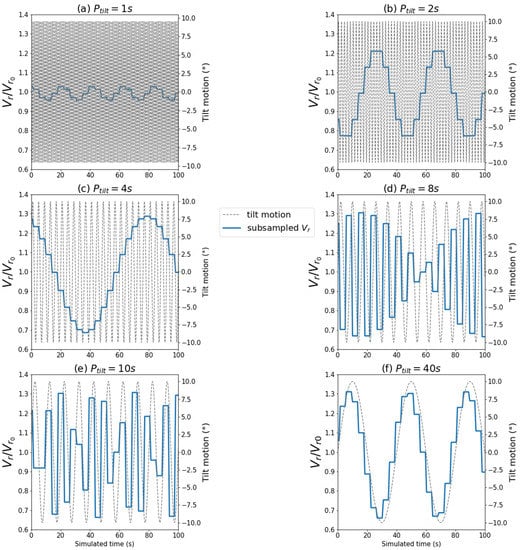
Figure 9.
Example of the subsampling and averaging effect on the radial wind speed measurement of beam A described in Section 4.2.2 subjected to a sinusoidal tilt of amplitude . The radial wind speed measured by the ray (in blue) is normalized by the value measured in a motionless case . Different periods of tilt are evaluated: P = 1 s (a), 2 s (b), 4 s (c), 8 s (d), 10 s (e), 40 s (f). The tilt motion is displayed (in grey), the scale of the motion is displayed on the right hand side of the figures.
For motion periods , we see that the period of the measured radial wind speed signal is larger than the period of the tilt motion. The radial wind speed is affected by a subsample of the motion. For motion periods , harmonics due to the subsampling phenomenon are introduced but the period of the motion is respected by the radial wind speed measurements. These harmonics affect the standard deviation of the measurement and may also change the mean value of the measurement. For the period , the period of the motion is sufficiently greater than the period of one rotation of the LIDAR beam for the two signals to follow the same evolution.
4.2.5. Influence of a 10-min Sinusoidal Motion on the Measurement of the Entire LIDAR
The floating LIDAR measurement of a component of the horizontal wind is calculated from the radial speed measurements of two opposite rays. Thus, the horizontal speed is calculated from the measurement of the four non-vertical rays. As the radial velocities are measured alternately, they do not experience the same motion. At the scale of a 10-min measurement, each ray experiences a different subsampling of the LIDAR motion. In this section, we consider sinusoidal tilt, yaw and heave motions. The heave was chosen to represent the effect of translational velocity as it is the component with the greatest impact on the horizontal velocity measurement [16]. As in the WindCube v2® operation, we compute the lidar measurement statistics from the recorded data from each LOS measurement. We normalize the velocities and standard deviations evaluated throughout this section by the incident horizontal wind speed . All the simulations in this section are carried out under similar wind conditions ().
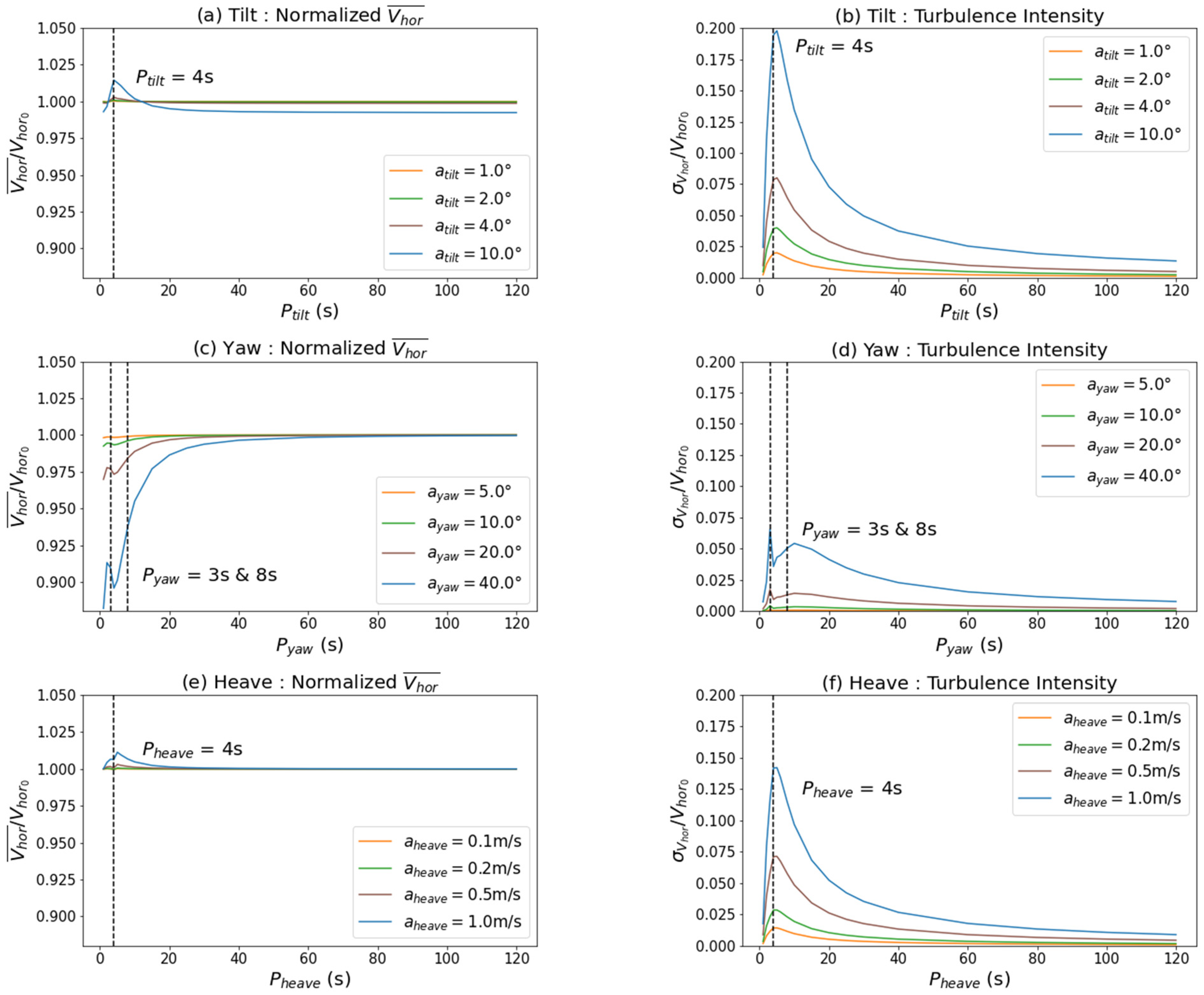
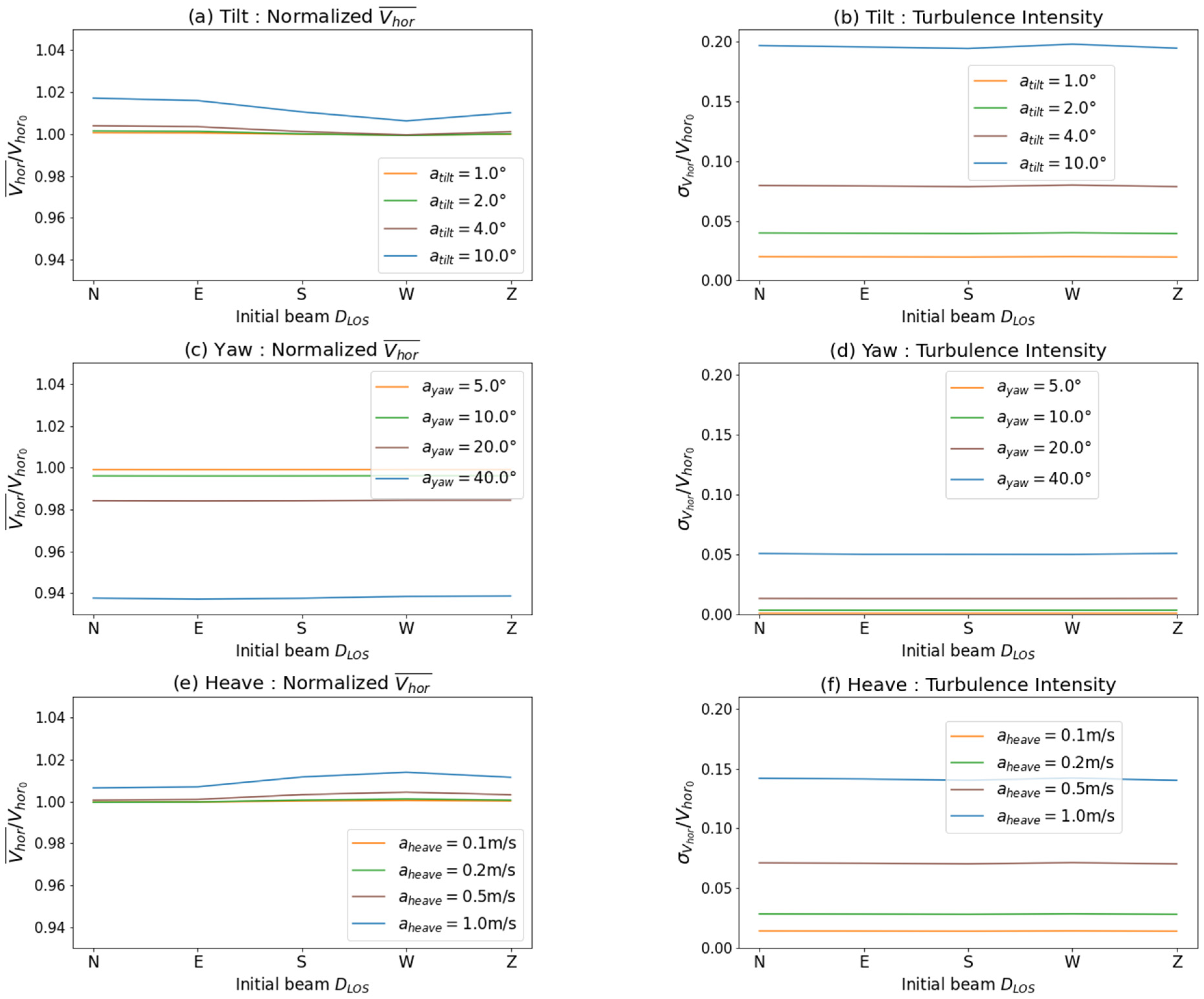
Figure 10 and Figure 11 show the influence of the period of the sinusoidal motion, and the direction of the initial beam in the model, respectively. The mean horizontal velocities and standard deviations are compared. Since the incident horizontal velocity is turbulence-free, the calculated standard deviation is entirely induced by the motion. The effect of the initial direction of the laser beam is evaluated at the period having the greatest impact on the LIDAR measurement, called resonance period. We discuss all the figures according to the type of motion: tilt, yaw and heave. Finally, we study the dominant effects on the LIDAR error as a function of sea conditions.
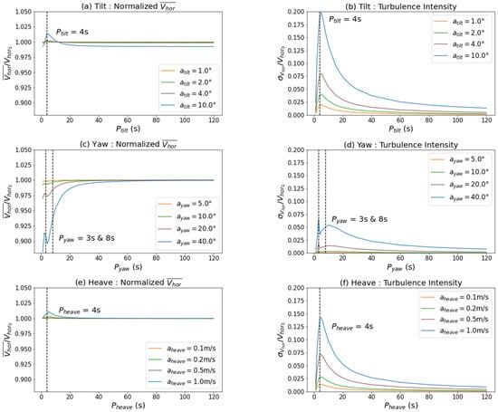
Figure 10.
Influence of the period of a sinusoidal motion on the mean horizontal velocity and its standard deviation estimated by the model and normalized by the incident horizontal velocity . The periods having the greatest impact on the LIDAR measurement, called resonance period, are specified. (a,b) LIDAR subjected to a sinusoidal tilt motion for an incident wind along the component perpendicular to the axis of rotation. (c,d) LIDAR subjected to a sinusoidal yaw motion. (e,f) LIDAR subjected to a sinusoidal heave motion.
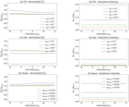
Figure 11.
Influence of direction of the initial beam within the model on the mean horizontal wind speed and its standard deviation estimated by the model and normalized by the incident horizontal speed . (a,b) LIDAR subjected to a sinusoidal tilting motion of period = 4 s for an incident wind along the component perpendicular to the rotation axis. (c,d) LIDAR subjected to a sinusoidal yaw motion of period = 3 s. (e,f) LIDAR subjected to a sinusoidal heave motion of period = 4 s.
We start with the tilt motion, it is applied in the axis perpendicular to the incident wind direction (i.e., roll for ). The average horizontal velocity measurement (Figure 10a) evaluated by the model is either smaller or greater than the incident horizontal wind speed as a function of the tilt period. The error induced by an extreme motion () is up to 1 to 2% at the resonance period , the initial direction of the measurement beam in the model strongly influences the magnitude of this error (Figure 11a).
The standard deviation of the horizontal velocity (Figure 11b) fluctuates with the period and amplitude of the motion, reaching its maximum value at the resonance period . The order of magnitude of the TI induced by an extreme motion is 0.2 at the resonance period. The standard deviation of the horizontal velocity is only slightly influenced by the initial direction of the beam (Figure 11b).
Now, we study the effect of yaw motion. It has a similar influence on all the 4 non-vertical beams. However, the difference in the timing of evaluations introduces a compositional effect between the subsampling encountered by each ray. The average horizontal velocity measurement evaluated by the model (Figure 10c) is always lower than the horizontal incident wind speed . The underestimation for a yaw at resonance periods ( = 3 s & 8 s) and amplitude = 40° is of the order of 10%.
The standard deviation of the horizontal velocity (Figure 10d) varies with the period and amplitude of the sinusoidal motion, its maximum value being encountered at the resonance period = 3 s. The order of magnitude of the motion-induced TI for a tilt amplitude = 40° is about 0.05 at the resonance periods.
The initial direction of the beam in the model has little influence on the horizontal velocity measurement of the floating LIDAR in the case of yaw motion (Figure 11c,d). And we specify that the case studied here of a yaw of high amplitude evolving at high frequency was not encountered in our experimental study (Section 4.1). The measured yaw from the WINDSEA_02 buoy shows a high amplitude/low frequency in calm sea conditions and a low amplitude/high frequency in rough sea conditions.
Now, we focus of the effect of heave. The translational movements of the buoy appear as an added component to the velocity vector measured by the LIDAR. The difference in the temporality of the evaluations introduces a compositional effect between the subsamples encountered by the rays. The average horizontal velocity measurement (Figure 10e) evaluated by the model is always higher than the horizontal incident wind speed . The overestimation for a heave at resonance period ( = 4 s) and amplitude = 1 m/s is of the order of 1%, the initial direction of the ray strongly influences the magnitude of this error (Figure 11e).
The standard deviation of the horizontal velocity (Figure 10f) varies with the period and amplitude of the sinusoidal motion, the maximum value is encountered at the resonance period. The order of magnitude of the motion-induced TI for a tilt amplitude = 1 m/s is 0.15 at the resonance period. The initial direction of the beam has little effect on the standard deviation of the horizontal velocity estimated by the model (Figure 11f).
Now, we want to assess the motions with the greatest impact on the LIDAR measurement in different sea conditions. The horizontal wind speed measured by a LIDAR subjected to a tilt, yaw or heave motion depends on the period of the motion. Resonance periods are observed for each of these phenomena. Each of the observed resonance period are close to the time required for the LIDAR to perform a LOS measurement for each of its beams (~4 s). The initial direction of the measuring beam also has an influence on the average value of the horizontal velocity for tilt and heave. In the context of our turbulence intensity measurement correction method presented in Section 3.1, we note that the default choice of the first measuring ray influences the value of . The standard deviation of the horizontal velocity is only slightly influenced by the initial direction of the ray. However, this quantity is by definition linked to the average horizontal velocity.
We shall study the order of magnitude of the motion-induced bias on the LIDAR measurement as a function of the sea conditions presented in Section 4.1. We note that the turbulence intensity value presented here corresponds to the motion-induced TI evaluated in a turbulence-free atmosphere, it should not be added to the atmospheric turbulence as a bias, the relationship is quadratic (Equation (9)).
In calm sea conditions, the three motions lead to motion-induced TI of the same order of magnitude (0.01 to 0.04) and the horizontal speed is mainly impacted by the yaw (relative underestimation of about 1%). The initial direction of the beam has little influence on the average horizontal wind value.
In rough sea conditions, yaw has very little influence on the horizontal wind measurement. The tilt and heave motions cause a huge motion-induced TI of the same order of magnitude (0.1 to 0.2). As a comparison, atmospheric turbulence intensities exceeding 0.1 are very rare in an open sea area [23,24]. The mean horizontal velocity is also impacted by tilt and heave motions with a relative overestimation of the order of 1 to 2%, corroborating the order of magnitude of error reported by Gottschall et al. [15].
4.3. Influence of Wave-Induced Motion on the Experimental TI Measurement of the WindCube v2® in Fécamp
In an experimental situation, the errors induced by the different degrees of freedom of motion of the LIDAR overlap. They add up in some cases and cancel each other out in others. This is the reason why it is essential to use a model that takes into account each degree of freedom of the buoy and their interactions, in order to accurately estimate the magnitude of the LIDAR’s motion-induced error. We first study the wave-induced turbulence intensity measurement error. Then, we apply the correction to the experimental data set.
We note that the data measured at Fécamp belong to EDF Renouvelables and cannot be made public. We normalize the mean wind and turbulence intensity data set by the mean value of the validation data (anemometer or fixed LIDAR). The absolute error of the turbulence intensity and the regression equations are calculated from the non-normalized data to preserve the physical meaning.
4.3.1. Study of Wave-Induced TI Experimental Error
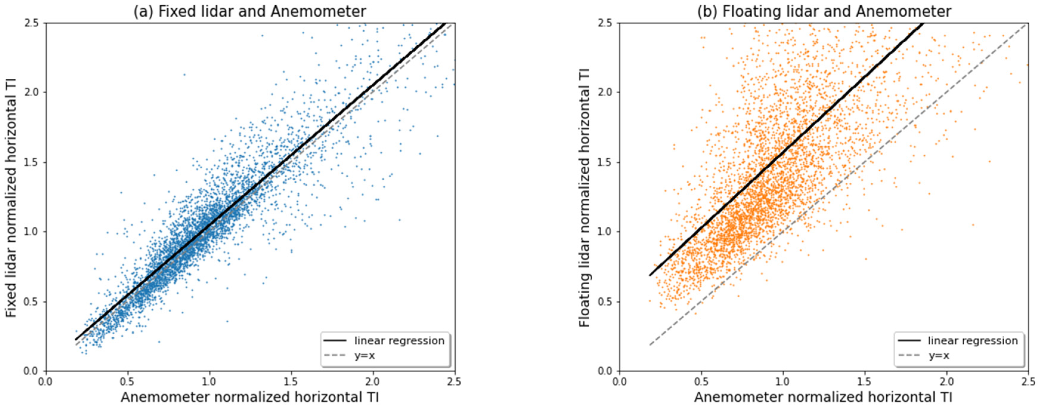
The operating principle of the profiler LIDAR technology induces a bias in the turbulence intensity measurement compared to anemometers [9]. In the open sea conditions of Fécamp, the regression line on the non-normalized data from the fixed LIDAR follows the equation: (Figure 12a). The TI measurement of the fixed LIDAR is on average similar to that of the anemometer. However, the dispersion of the points is very large. This divergence is due to the difference in technology and to the low measurement altitude (54.8 m relative to MSL, i.e., about 40 m from the fixed LIDAR) that affects the LIDAR measurement accuracy [20].
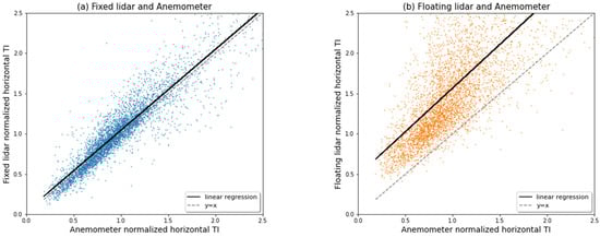
Figure 12.
Linear regression of turbulence intensity measurements by the fixed (a) and floating (b) LIDARs in comparison with the cup anemometer measurements, at altitude 54.8 m. The ticks are normalized by the anemometer mean TI from all the 10-min samples.
In the case of the floating LIDAR, the effect of wave motion induces a much larger error (Figure 12b). The regression line on the non-normalized data follows the equation: .
The slope is close to unity, but the value at the origin is non-zero, which means that buoyancy motion introduces an offset of the order of +0.03. The dispersion of the points is also accentuated by the wave motion.
We conclude that the wave-induced error is much greater than the technological error from the LIDAR when compared to a cup anemometer. In the remainder of this section, we compare the floating LIDAR measurements with the fixed LIDAR measurements in order to evaluate the effect of waves with equivalent technology.
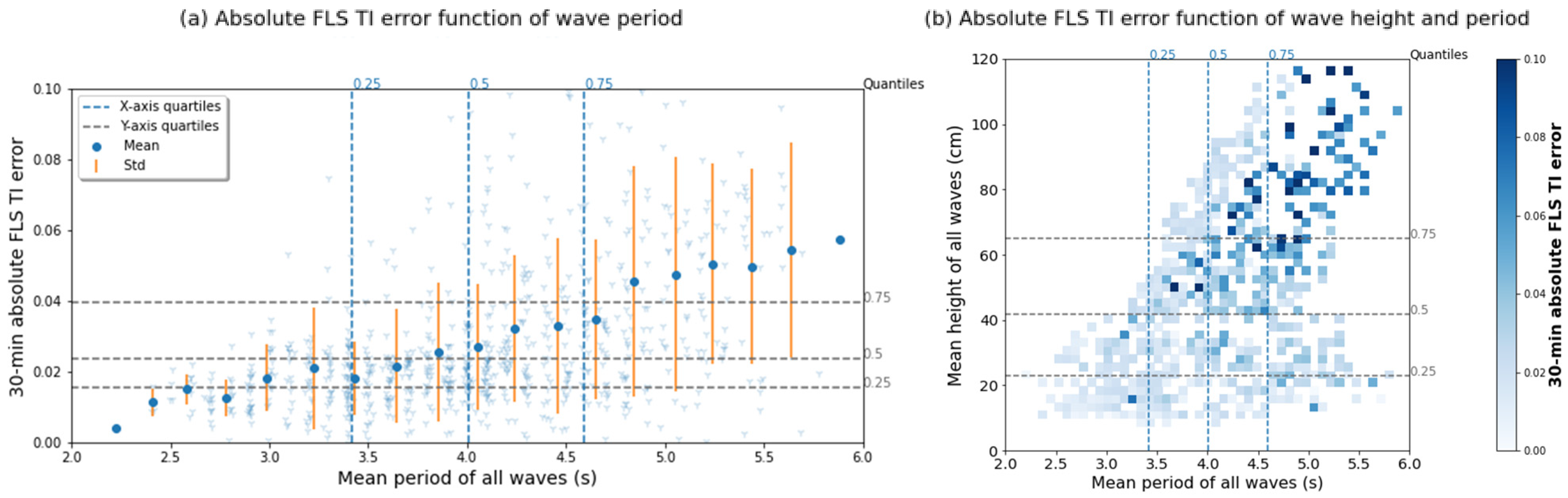
From the wind, wave and atmospheric data used to select the 13 weeks out of the overall measurement campaign (Section 3.2), we performed a parametric study correlating the met-ocean conditions with the floating LIDAR turbulence intensity measurement error. The most highly correlated data with the floating LIDAR measurement error is the wave period (Figure 13a), which is itself closely correlated with both wave height (Figure 13b) and wind speed. In Figure 13a, we observe that for any average wave period within a 30-min interval, the mean error in the TI measurement is always significant (>0.01). Therefore, low wave periods induce sufficient motion to the WINDSEA_02 buoy to have a substantial impact on the LIDAR turbulence intensity measurement. We note that this result is highly dependent on the dynamic response of the buoy to waves, for example, the buoy used in Gottschall et al. [17] experiences a weaker response to low waves. We also note that, in our case, very low wave heights are filtered out by the /s condition.
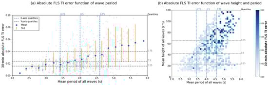
Figure 13.
Distribution of the floating LIDAR TI absolute measurement error as a function of the 30-min wave statistics measured by the wave buoy. The turbulence intensity measurement error (absolute discrepancy) of the FLS is evaluated on the 10-min data in comparison to the fixed LIDAR at the altitude of 94.4 m. The 10-min data is averaged over 30 min for correlation with the 30-min wave statistics. Quartiles are displayed as dash lines for visualizing the statistical distribution of the data. (a) 30-min absolute FLS TI error as a function of the mean period of all waves. (b) Colormap of the 30-min absolute FLS TI measurement error with respect to the wave mean period and height.
We now analyze in detail the floating LIDAR measurement error during the Fécamp campaign. By studying the origin of the wind in the reference frame of the LIDAR (and the buoy) (Figure 14a), we can observe that the dominant component of the wind is coming from the east. Furthermore, in our previous study (Section 4.2.3), we observed that the dominant motions in the LIDAR measurement error in rough seas are tilt and heave. Thus, the tilt motion whose axis is perpendicular to the wind source (the roll) is the dominant rotational motion in the turbulence intensity measurement error. Figure 14b confirms this trend: It shows a very strong correlation between roll, mean wind speed and the floating LIDAR measurement error. The trend is less apparent for translational movements because the components involved in the heave motion are affected by the rotation of the buoy.
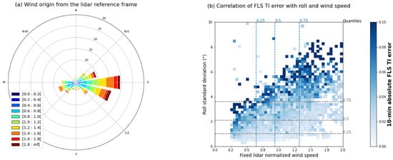
Figure 14.
Study of the dominant phenomenon in the turbulence intensity measurement error of the floating LIDAR on the Fécamp site. (a) Origin of the winds in the floating LIDAR reference frame, the color scale designates the normalized horizontal speed. (b) Colormap of the absolute TI measurement error of the floating LIDAR with respect to the fixed LIDAR as a function of roll standard deviation (in degrees) and normalized mean wind speed.
This macroscopic method allows us to understand a part of the behavior of the floating LIDAR measurements. However, a mathematical model is mandatory in order to take into account all the geometrical effects and their mutual interactions.
4.3.2. Model-Based Correction of Turbulence Intensity Measurements
The model presented in Section 3.1 is applied to the experimental data in order to estimate the atmospheric turbulence from the floating LIDAR and the IMU. The gyroscopic and translational data are linearly interpolated to fit the 10 Hz discretization defined in the model. The initial measurement beam is defined in the North direction of the LIDAR, by default.
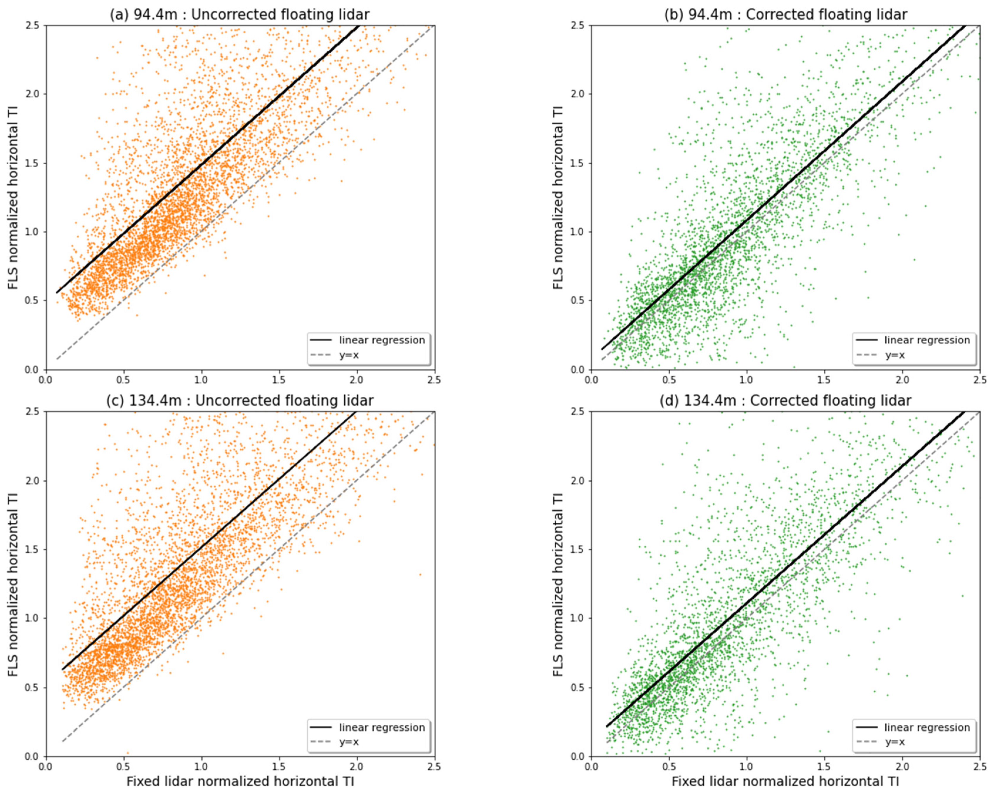
Figure 15 shows the linear regression of the uncorrected and corrected turbulence intensity estimates for the entire 10-min data set evaluated during the 13 weeks of experimental data. At elevation 94.4 m (Figure 15a,b), the regression lines on the non-normalized data follow the equations: and . The model compensates for most of the mean bias introduced by wave motion: the slope of the curve changes little, but the value at the origin shifts from 0.032 without correction to 0.005 with correction. The dispersion of the data points is also impacted, it shifts from 0.673 without correction to 0.731 with the correction. At elevation 134.4 m (Figure 15c,d), the regression lines on the non-normalized data follow the equations: and . The trend is similar to altitude 94.4 m, but the average bias of the corrected measurement is slightly larger for elevation 134.4 m.

Figure 15.
Linear regression of the 10-min turbulence intensity measurement from the uncorrected and corrected floating LIDAR with respect to the fixed LIDAR measurement at two altitudes: 94.4 m and 134.4 m. All ticks are normalized by the fixed LIDAR’s mean TI from all the 10-min samples. (a,c) Raw floating LIDAR measurement at the two evaluated altitudes. (b,d) Floating LIDAR measurement corrected by the model at the two evaluated altitudes.
We note that the number of data is affected by the use of the model. The correction acts as a filter in the case of a negative motion-induced variance calculated by Equation (21). This situation occurs for 10-min samples lacking consistency between IMU and LIDAR measurements and/or not meeting model assumptions. From the 13 weeks of data selected, about 33% of the data are filtered out by the model (1738/5223 at altitude 94.4 m).
Figure 16 shows the effect of the model-based correction on the time series of the harshest week (from 06/24/18 to 07/01/18). Without correction, we observe a large variation in the error of the floating LIDAR turbulence intensity measurement in a day, which is related to the variation of the wave period. The estimation of atmospheric turbulence by the model allows us to correct most of 10-min measurements. However, some corrected data still strongly overestimate the turbulence intensity (Figure 16b). As these points are mostly isolated, a peak filter can be easily applied to discard them and improve the performance of the correction. In particular, we draw the reader’s attention to the filter presented by Wang et al. [25], which removes the removal of isolated peaks.
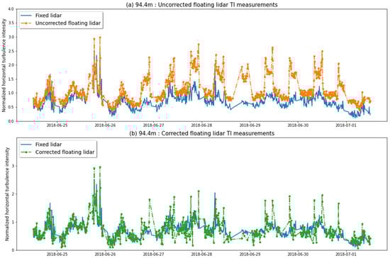
Figure 16.
Effect of the model-based correction of the turbulence intensity measurement for the harshest week of the overall 13 (from 06/24/18 to 07/01/18). FLS measurements are compared with the fixed LIDAR measurements. All samples are normalized by the mean value from the fixed LIDAR. (a) Uncorrected floating LIDAR measurement. (b) Corrected measurement using the 10-min model-based correction presented in Section 3.1.
5. Conclusions
Using the model developed in this paper, we have investigated in detail the mechanisms responsible for the turbulence intensity measurement error of a floating LIDAR. The sea conditions influence the dynamic response of the buoy and consequently the turbulence intensity measurement of the FLS. In the search to elaborate the error of the LIDAR, we reviewed the most significant of the six degrees of freedom of motion on the LIDAR measurement behavior. Then, from the knowledge of the origin of the wind in the LIDAR frame of reference, we deduce the motions affecting the most the LIDAR measurement as well as the order of magnitude of the induced errors. On the WINDSEA_02 buoy in rough sea conditions, tilting and heaving are the most significant motions affecting the LIDAR measurement of turbulence intensity. This is due to the modification of the cone geometry, and the translation velocity appearing as an added component to the velocity vector, respectively.
During the experimental campaign in Fécamp, the motion-induced turbulence intensity measurement error of the floating LIDAR is an overestimate of 0.03 when compared to a cup anemometer (or a fixed LIDAR) over the 13 selected weeks. Based on a correlation study of the FLS error with the met-ocean conditions, we determined that the most correlated physical phenomenon with the FLS measurement error is the wave period, which is closely correlated with wave height and wind speed. However, no met-ocean conditions can ensure a zero error in the floating LIDAR turbulence intensity measurement for this specific buoy. Therefore, it is essential to correct the FLS TI measurement.
The model-based method estimates the atmospheric turbulence intensity from 10-min floating LIDAR data and the six degrees of freedom time series of an IMU. Based on computationally efficient calculations relative to existing methods, it simulates the behavior of a profiler LIDAR and evaluates the impact of rotational and translational motions on the measured radial velocities. The method efficiently corrects the TI measurements of the floating LIDAR deployed at Fécamp for most of the 10-min estimates, allowing a satisfactory linear regression to be reached with respect to the fixed LIDAR measurements. The 10-min estimates that are still overestimated after using the model are generally isolated, allowing a peak filter to discard them.
Further research should investigate sea-induced motions on buoys of different sizes and dynamic responses in order to gain a more comprehensive understanding of the relationship between sea conditions, buoy behavior and FLS turbulence intensity measurement errors. The model could be improved by a boundary layer shear, which would significantly complicate the matrix system. The model could also be adapted to the correction of CW LIDAR measurements.
Author Contributions
Conceptualization, T.D.; data curation, T.D.; formal analysis, T.D.; funding acquisition, S.A.; investigation, S.A.; methodology, T.D.; project administration, S.A.; software, T.D.; supervision, S.A. and G.K.; visualization, T.D.; writing—original draft, T.D.; writing—review and editing, T.D., S.A., and G.K. All authors have read and agreed to the published version of the manuscript.
Funding
This work was carried out within the framework of the WEAMEC, West Atlantic Marine Energy Community, and with funding from the Pays de la Loire Region.
Acknowledgments
We acknowledge EDF Renouvelable® and AKROCEAN® for providing the experimental data from the campaign of Fécamp. We would like to thank all the people involved in the MATILDA project: Phillipe Baclet (WEAMEC®), Samy Kraiem (CSTB), Romain Barbot and Lise Mourre (VALOREM®), Benoit Clauzet (EDF Renouvelables®), Maxime Bellorge (AKROCEAN®) We also like to thank Paul Mazoyer and Andrew Black from Leosphere®, that took the time to answer our questions on the WindCube v2® operation.
Conflicts of Interest
The authors declare no conflict of interest. The funders had no role in the design of the study; in the collection, analyses, or interpretation of data; in the writing of the manuscript, or in the decision to publish the results.
Appendix A
Development of the and components used for variance estimator calculation (Equation (21)):
with and beign respectively the components of the vectors and (Equation (20)).
References
- Pantaleo, A.; Pellerano, A.; Ruggiero, F.; Trovato, M. Feasibility study of off-shore wind farms: An application to Puglia region. Sol. Energy 2005, 79, 321–331. [Google Scholar] [CrossRef]
- Mücke, T.; Kleinhans, D.; Peinke, J. Atmospheric turbulence and its influence on the alterning loads on wind turbines. Wind Energy 2011, 14, 301–316. [Google Scholar] [CrossRef]
- Frehlich, R.; Meillier, Y.; Jensen, M.L.; Balsley, B.; Sharman, R. Measurements of boundary layer profiles in an urban environment. J. Appl. Meteorol. Climatol. 2006, 45, 821–837. [Google Scholar] [CrossRef]
- Hall, F.F.; Huffaker, R.M.; Hardesty, R.M.; Jackson, M.E.; Lawrence, T.R.; Post, M.J.; Richter, R.A.; Weber, B.F.; Hall, J. Wind measurement accuracy of the NOAA pulsed infrared Doppler lidar. Appl. Opt. 1984, 23, 2503–2506. [Google Scholar] [CrossRef] [PubMed]
- Banta, R.; Darby, L.S.; Kaufmann, P.; Levinson, D.H.; Zhu, C.-J. Wind-Flow Patterns in the Grand Canyon as Revealed by Doppler Lidar. J. Appl. Meteorol. 1999, 38, 1069–1083. [Google Scholar] [CrossRef]
- Peña, A.; Gryning, S.E.; Hasager, C.B. Measurements and modelling of the wind speed profile in the marine atmospheric boundary layer. Bound. Layer Meteorol. 2008, 129, 479–495. [Google Scholar] [CrossRef]
- Peña, A.; Hasager, C.B.; Gryning, S.-E.; Courtney, M.; Antoniou, I.; Mikkelsen, T. Offshore wind profiling using light detection and ranging measurements. Wind Energy 2009, 12, 105–124. [Google Scholar] [CrossRef]
- Kindler, D.; Oldroyd, A.; Macaskill, A.; Finch, D. An eight month test campaign of the QinetiQ ZephIR system: Preliminary results. Meteorol. Z. 2007, 16, 479–489. [Google Scholar] [CrossRef]
- Sathe, A.; Banta, R.; Pauscher, L.; Vogstad, K.; Schlipf, D.; Wylie, S. Estimating Turbulence Statistics and Parameters from Ground- and Nacelle-Based Lidar Measurements. In IEA Wind Expert Report; DTU Wind Energy: Roskilde, Denmark, 2015. [Google Scholar]
- Sathe, A.; Mann, J.; Gottschall, J.; Courtney, M. Can Wind Lidars Measure Turbulence? J. Atmos. Ocean. Technol. 2011, 28, 853–868. [Google Scholar] [CrossRef] [Green Version]
- Sjöholm, M.; Mikkelsen, T.; Mann, J.; Enevoldsen, K.; Courtney, M. Spatial averaging effects on turbulence measured by a continuous-wave coherent lidar. Meteorol. Z. 2009, 18, 281–287. [Google Scholar] [CrossRef]
- Newman, J.F.; Klein, P.M.; Wharton, S.; Sathe, A.; Bonin, T.; Chilson, P.B.; Muschinski, A. Evaluation of three lidar scanning strategies for turbulence measurements. Atmos. Meas. Tech. 2016, 9, 1993–2013. [Google Scholar] [CrossRef] [Green Version]
- Kelberlau, F.; Mann, J. Cross-contamination effect on turbulence spectra from Doppler beam swinging wind lidar. Wind Energy Sci. 2020, 5, 519–541. [Google Scholar] [CrossRef]
- Sathe, A.; Mann, J. Measurement of turbulence spectra using scanning pulsed wind lidars. J. Geophys. Res. 2012, 117, D01201. [Google Scholar] [CrossRef] [Green Version]
- Gottschall, J.; Gribben, B.; Stein, D.; Würth, I. Floating lidar as an advanced offshore wind speed measurement technique: Current technology status and gap analysis in regard to full maturity. WIREs Energy Environ. 2017, 6, e250. [Google Scholar] [CrossRef]
- Kelberlau, F.; Neshaug, V.; Lønseth, L.; Bracchi, T.; Mann, J. Taking the Motion out of Floating Lidar: Turbulence Intensity Estimates with a Continuous-Wave Wind Lidar. Remote Sens. 2020, 12, 898. [Google Scholar] [CrossRef] [Green Version]
- Gottschall, J.; Wolken-Möhlmann, G.; Viergutz, T.; Lange, B. Results and conclusions of a floating-lidar offshore test. Energy Procedia 2014, 53, 156–161. [Google Scholar] [CrossRef]
- Mann, J.; Peña, A.; Bingöl, F.; Wagner, R.; Courtney, M. Lidar Scanning of Momentum Flux in and above the Atmospheric Surface Layer. J. Atmos. Ocean. Technol. 2010, 27, 959–976. [Google Scholar] [CrossRef]
- Lindelöw, P. Fiber Based Coherent Lidars for Remote Wind Sensing. Ph.D. Thesis, Danish Technical University, Kgs. Lyngby, Denmark, 2008. [Google Scholar]
- Cariou, J.P.; Boquet, M. LEOSPHERE Pulsed Lidar Principle. In Contribution to UpWind WP6 on Remote Sensing; LEOSPHERE: Orsay, France, 2010. [Google Scholar]
- Edson, J.B.; Hinton, A.A.; Prada, K.E.; Hare, J.E.; Fairall, C. Direct Covariance Flux Estimates from Mobile Platforms at Sea. J. Atmos. Ocean. Technol. 1998, 15, 547–562. [Google Scholar] [CrossRef] [Green Version]
- Yuan, C.; Yang, H. Research on K-Value Selection Method of K-Means Clustering Algorithm. J 2019, 2, 226–235. [Google Scholar] [CrossRef] [Green Version]
- Türk, M.; Emeis, S. The dependence of offshore turbulence intensity on wind speed. J. Wind Eng. Ind. Aerodyn. 2010, 98, 466–471. [Google Scholar] [CrossRef]
- Argyle, P.; Watson, S.; Montavon, C.; Jones, I.; Smith, M. Modelling turbulence intensity within a large offshore wind farm. Wind Energy 2018, 21, 1329–1343. [Google Scholar] [CrossRef]
- Wang, H.; Barthelmie, R.J.; Clifton, A.; Pryor, S.C. Wind measurements from arc scans with Doppler wind lidar. J. Atmos. Ocean. Technol. 2015, 32, 2024–2040. [Google Scholar] [CrossRef]


Publisher’s Note: MDPI stays neutral with regard to jurisdictional claims in published maps and institutional affiliations. |
© 2021 by the authors. Licensee MDPI, Basel, Switzerland. This article is an open access article distributed under the terms and conditions of the Creative Commons Attribution (CC BY) license (https://creativecommons.org/licenses/by/4.0/).