Abstract
A directional borehole radar consists of one transmitting antenna in the borehole and four receiving antennas distributed at equal angles in a ring. The receiving antennas can determine the depth and orientation of targets beside the borehole. However, the problem of target orientation determination and 3D imaging algorithms remains a technological challenge. The MUSIC (multiple signal classification) algorithm requires a peak search, so the accuracy of the operation is limited by the angle interval. Based on the MUSIC algorithm, the Root-MUSIC algorithm is proposed and implemented. By replacing the spectral peak search with calculating the roots of the polynomials greatly improves the orientation recognition accuracy. Finally, the results obtained using the above algorithm are verified with synthetic data and compared with the results of the MUSIC algorithm. The results show that both the MUSIC algorithm and the Root-MUSIC algorithm can achieve very good orientation determination and 3D imaging results. In terms of accuracy, the Root-MUSIC algorithm has an obvious improvement compared with the MUSIC algorithm.
1. Introduction
GPR (Ground penetrating radar) is an effective spherical physical method to detect targets by using the electrical properties of underground media [1]. It mainly detects the underground electrical targets by transmitting and receiving high frequency electromagnetic waves [1]. When an electromagnetic wave propagating in underground media interfaces a medium with different electromagnetic characteristics, it is reflected. After the returned electromagnetic wave is received, a radar time profile is formed by processing the signal. According to the parameters of signal intensity, waveform, and double travel time in the profile, the spatial position, electrical state, and geometry of the target can be detected. GPR is widely used in many fields, such as groundwater pollution research, geotechnical engineering, sedimentology, glaciology, and archaeology [2,3,4].
A GPR system includes a transmitting antenna and receiving antennas, as well as a control system for receiving and transmitting signals and data storage. GPR uses wide-band antennas [5,6]. Different antennas have different frequency ranges, detection depths, and resolutions. When GPR uses a lower frequency wave, the detection depth can be larger, but the resolution is relatively low; conversely, when using a higher frequency electromagnetic wave, the detection depth is shallow, but the resolution is relatively high [7].
Borehole radar is a type of GPR, and because the antennas are placed in the borehole, it can detect and evaluate the geological structure of deep underground areas with a high resolution [8]. The application of borehole radar includes underground structure detection, feature description, geological research, and underground facilities detection. At present, the antenna frequency of borehole radar is generally lower than 100 MHz, and the penetration depth in crystalline rock is 20 m or more [9,10].
The traditional borehole radar transmitting antenna and receiving antennas are omni-directional, so they can only detect the depth of the target and the distance to the borehole, but not its azimuth [11]. At present, three-dimensional imaging of underground media is still very difficult. To solve this problem, directional borehole radar technology has been developed [12].
Directional borehole radar can detect not only the depth and distance from the target but also its azimuth [13,14,15]. There are two ways to realize the directional borehole radar: the first is to use array antennas to receive the measurement, which uses the uniform circular array to extract the azimuth information according to the different arrival times [16]; the second is to use a directional transmitting antenna, which directionally transmits the electromagnetic wave around the borehole, and the azimuth of the target is found from the transmitting direction of the antenna [17]. In a conventional borehole radar system, the transmitting antenna emits an electromagnetic wave isotropically, i.e., without special directivity. However, in a borehole radar system with a directional transmitting antenna, it is necessary to ensure the transmitting antenna has clear directivity to accurately determine the orientation of the target through the reflected wave [18,19,20].
For directional transmitting antenna, we need a directional antenna. Generally speaking, an underground antenna is composed of an electric dipole or a magnetic dipole. Whether it is an electric dipole or a magnetic dipole, the radiation of the antenna is omnidirectional in the direction of the borehole axis rotation. In order to solve the problem of reflector accurate positioning, it is necessary to research and develop the asymmetric antenna around the borehole axis, namely the directional antenna. The antenna can indicate the orientation of the reflector. Jeffrey Lytle of Lawrence Livermore Laboratory at the University of California, in the United States, was the first to carry out research in this field. They have developed an antenna whose point source is eccentrically located in a high dielectric constant medium. Due to the eccentric effect of the source, the radiation of the antenna is not axisymmetric in the direction of rotation. However, the study did not provide the measured data. Wright and others from the U.S. Geological Survey have also carried out a lot of research and developed a prototype of the directional radar system. The antenna is composed of a monopole antenna placed in a cavity. The effectiveness of the antenna is verified by numerical simulation and physical experiments. The results show that the antenna has azimuth directivity, but some backward radiation is unavoidable. T and amp; a radar from the Netherlands is the company’s in-hole directional radar system. They placed a reflector behind a dipole antenna and filled it with special materials to form a directional antenna. This kind of antenna is a bit like the shielding antenna of GPR. The directivity of a high-frequency range antenna is easy to obtain, but the penetration ability of these frequencies is poor. Therefore, in the development process, we need to take a compromised method to ensure penetration and directivity at the same time. This determines the size of the antenna and the size of the probe. The antenna is optimized for a 100 MHz measurement. Another related problem is the consideration of the whole module and durability, so as to produce a simple and flexible instrument. These considerations lead to the complete separation of the positioning system of the probe from the actual radar system. The radar system is located in the cylindrical radar module, which includes two antennas and all electronic components. The module itself cannot determine the orientation of the probe itself and cannot resist large pressure and external temperature. The positioning module is used to determine the position of the probe itself. It consists of a motor and a position detector with the entire antenna in it. The positioning module protects the radar module from the harsh underground environment [21].
Directional receiving borehole radar is more common than directional transmitting antenna radar [22]. For this kind of directional receiving antenna, one transmitting antenna and four receiving antennas are used, as shown in Figure 1. The four antennas are distributed uniformly along a ring perpendicular to the borehole. For the convenience of analysis, the four antennas are labeled East, South, West, and North, rotating clockwise. When the direction of the North antenna is consistent with the geographical North, the other antennas are consistent with the geographic East, West, and South; otherwise, a deviation angle exists that can be corrected by measuring the angle between the North antenna and the geographical North. Therefore, only the azimuth relative to the four antennas is needed to calculate the azimuth of the target. We compare and analyze the waveforms received by the four receiving antennas, use the corresponding azimuth estimation algorithm to determine the specific azimuth of the target, and then use the azimuth to carry out three-dimensional imaging of the target.
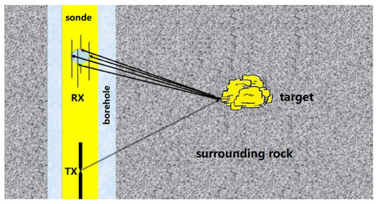
Figure 1.
Single-transmitter four-receiver borehole radar.
The MUSIC (multiple signal classification) algorithm, the traditional azimuth recognition algorithm, uses the orthogonality of signal subspace and noise subspace to construct the spatial spectrum [23]. A certain angle interval is selected to search the spectrum peak, which corresponds to the direction of the reflected wave. Therefore, the accuracy of the MUSIC algorithm is limited by the angle interval. This paper proposes and implements a three-dimensional imaging algorithm of directional borehole radar based on the Root-MUSIC algorithm. The Root-MUSIC algorithm is a kind of spatial spectrum algorithm that uses the process of calculating the roots of polynomials to replace the spectral peak search in the MUSIC algorithm. The accuracy of operation is not limited by the angle interval, so it is greatly improved.
2. Materials and Methods
2.1. Materials
In this paper, the FDTD (Finite Difference-Time Domain) algorithm is used to synthesize data. We use a two-dimensional model and a three-dimensional model for numerical simulation.
2.1.1. Two-Dimensional Model
The transmitting and receiving antennas used in this paper are both point antennas. As is shown in Figure 2, the size of the model on the x-axis and y-axis is 20 m × 20 m. The number of models in X and Y directions is 2000 × 2000. The size of the unit grid in the X and Y directions is 0.01 m × 0.01 m. In the process of the simulation, granite is selected as the surrounding rock, and its relative dielectric constant is 7; the fluid in the borehole is borehole water and the relative permittivity of it is 81; the relative permittivity of the sonde is 3; borehole radius is 5 cm; sonde radius is 4 cm; and, the array radius of the receiving antenna is 3 cm. When the receiving antenna array is placed between the borehole and the sonde, we change the azimuth of the transmitting antenna and calculate the azimuth of the transmitting antenna with the received signal. The transmitting antenna is 10 m away from the receiving antenna, so the incident wave can be regarded as a parallel wave. The following azimuth angles are used in this simulation: 24°, 166°, 196°, and 329°.
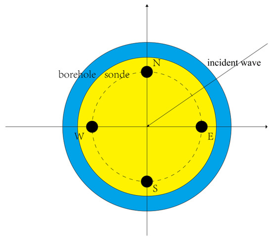
Figure 2.
Two-dimensional simulation model.
2.1.2. Three-Dimensional Model
The three-dimensional model is shown in Figure 3. The size of the model is 20 m × 20 m × 10 m. The number of cells in the main grid is 800 × 800 × 200, the grid size of the main grid is 0.025 m × 0.025 m × 0.05 m, and the sub-grid is from the 396th grid to the 405th grid in both the X- and Y-directions and from the 10th grid to the 190th grid in the Z-direction. The size ratio of the main grid to the sub-grid is 5:1.
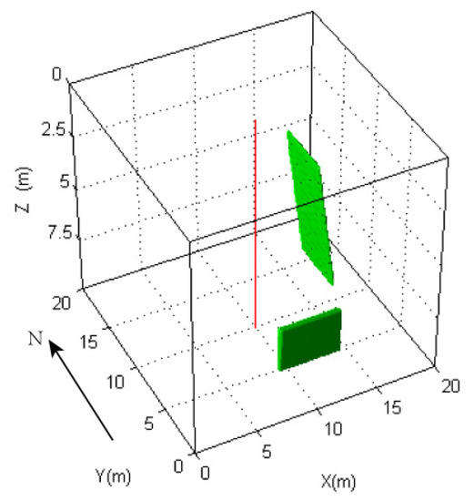
Figure 3.
Synthetic data model.
The model includes inclined fractures to the east of the borehole and vertical fractures to the south of the borehole. In the east direction, the top of the inclined fracture is 4.1 m away from the borehole with a depth of 2 m, and the bottom is 5.3 m away from the borehole with a depth of 8 m. The fracture is 5 m wide and 0.5 m thick. The diameter of the borehole is 10 cm, the diameter of the sonde is 8 cm, the receiving antennas are linear antennas of length 0.8 m, and the receiving and transmitting distance is 1.5 m. The fluid in the borehole is water. The sonde is made of PVC pipe. The surrounding rock is granite, and the fracture is filled with water. The physical parameters of the surrounding granite are as follows: the relative permittivity is 7, and the conductivity is 0.0007. The parameters of the water are as follows: the relative permittivity is 80, and the conductivity is 0.7. The parameters of the PVC pipe are as follows: the relative permittivity is 3, and the conductivity is 0.
2.2. Methods
2.2.1. Numerical Simulation Algorithm
The numerical simulation in this paper is essentially an electromagnetic phenomenon. The analysis of the electromagnetic problems is to solve the Maxwell equations under specific boundary conditions. Maxwell equations can be written in integral form and differential form. The time-domain finite difference method (FDTD) was first proposed by Kane. S. Yee [24]. It is based on the Maxwell curl equation in differential form, which can separate the differences between space and time. Previous studies have shown that FDTD is one of the most simple and effective numerical methods to calculate Maxwell equations, and it is a common calculation method for Directional Borehole Radar [25].
In this paper, the FDTD algorithm is used for numerical simulation. The FDTD algorithm transforms the Maxwell curl equation with the time variable into a different form and advances the solution of the space electromagnetic field in turn on the time axis. Each electric field (or magnetic field) component is surrounded by four magnetic fields (or electric fields) components. It is the simplest of all electromagnetic field calculation methods. It directly solves the problem from the Maxwell equation without complicated mathematical derivation and is quite intuitive and effective [26,27].
The traditional FDTD algorithm has the following problems. The first is the two-scale problem. When the scatterer is very small, it will lead to a two-scale problem. In order to simulate the geometry or internal structure of scatterers in detail, the size of the grid must be small enough, and the number of grids in the whole calculation area needs to be increased. When the model space is relatively large, the number of grids needed to solve this problem in the uniform grid space will be very large, which requires considerable memory consumption for the computer. The stability of FDTD is directly related to the time step, and the memory problem also makes the convergence slow. The second is that FDTD is difficult to work for curve boundary. In fact, FDTD only makes tensor product mesh, which can only get the surface target by ladder approximation [28].
To solve this kind of problem is to use a smaller mesh in the part that needs detailed simulation first and use the allowed coarse mesh for the rest. It can not only meet the calculation accuracy but also save memory and running time. This method is called sub-grid technology, also known as local fine grid technology, which is widely used in various problems. Intuitively, the whole region is calculated with the main grid, and then the sub-region is calculated with a smaller grid, and then the results of the two are combined [29,30].
The above is the numerical simulation method used in this paper. The following discusses the azimuth recognition and three-dimensional imaging algorithm used in this paper. Because the Root-MUSIC algorithm and the MUSIC algorithm involved in this paper are based on a uniform linear array, the general theory of uniform county is discussed first [31].
2.2.2. General Theory of Uniform Linear Array
We first discuss the relationship between an incident wave and a uniform linear array. The uniform linear array is a simple linear array, as shown in Figure 4. M elements are aligned along a line, and the element spacing is d. The DOA (Direction of Arrival) is defined as the angle between the wave direction and the array normal direction and is expressed as θ characterized by rotational symmetry around the array. The uniform linear array analysis is based on the following assumptions.
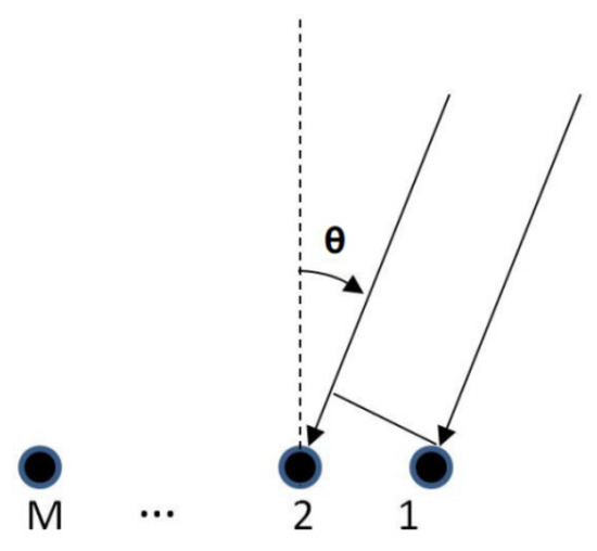
Figure 4.
Uniform linear array.
- (1)
- The number of sources cannot be greater than the number of receiving antennas;
- (2)
- The noise is uniform random noise, and the signal is not correlated with the noise;
- (3)
- The signal sources are usually narrow-band far-field signals;
- (4)
- The receiving antenna is omnidirectional and the mutual coupling between antennas is not considered [32,33].
If there are N(N < M) targets, the signal of the ith target is as follows:
where zi(t) is the complex envelope of the ith signal, which contains signal information; exp(jω0t) is the carrier of the spatial signal; ω0 is the angular frequency; and j is the imaginary unit. Then, the signal received by the whole antenna array is calculated as follows:
where is the array manifold, is the direction vector of the signal, is the time delay relative to the reference array element, is the signal matrix, is the additive noise matrix, and [•]T is the matrix transpose.
The time delay of the Mth element relative to the first element is shown below.
The direction vector of equidistant linear array is obtained as follows:
When the wavelength and the geometric structure of the array are determined, the direction vector is only related to the azimuth angle θ, so the direction vector of the equidistant linear array is denoted as , which is independent of the position of the reference point. If there are signal sources, the direction of arrival is , respectively.
The expression of the direction vector of an equidistant linear array is given above. The output of the antenna array is as follows:
The vector form is as follows:
where, is the weight vector.
2.2.3. Root-MUSIC Algorithm
The MUSIC algorithm uses the orthogonality of signal subspace and noise subspace to construct a spatial spectrum function. Through a spectrum peak search, the DOA of the signal is detected, and the peak corresponds to the target azimuth [34].
The MUSIC algorithm is based on the following assumptions:
- (1)
- The array element spacing is not less than half of the wavelength of the highest frequency signal;
- (2)
- The noise of the processor is additive Gaussian distribution;
- (3)
- The number of signal sources is less than the number of array elements, and the number of signal samples is greater than the number of array elements;
- (4)
- The source must be a random number with uniform distribution.
The Root-MUSIC algorithm first needs to define the following polynomial.
where is the eigenvectors corresponding to the small eigenvalues in the data covariance matrix, where
where . When the root of the polynomial is exactly on the unit circle, is a steering vector with spatial frequency ω. According to the eigenstructure algorithm, is the steering vector of the signal, so it is orthogonal to the noise subspace. Therefore, the definition of the polynomial can be modified as follows:
If roots of Equation (10) are obtained, the information about the angle of arrival of the signal sources can be obtained. At the same time, we find that there is a z* term in the polynomial, which makes the process of finding zero more complicated. If , then .
To simplify, Equation (10) is modified as follows:
To solve the problem conveniently, we continue to modify Equation (11) to obtain the modified Root-MUSIC algorithm expression.
Note that the order of the polynomial is , and the matrix has the property that there are pairs of complex roots mirrored symmetrical about the unit circle, and each pair of roots is conjugated with each other. Of these pairs of roots, there are N roots z1, ..., zN that are also exactly uniformly distributed on the unit circle, and
The above consideration is that the data covariance matrix can be known accurately. In practical applications, when there are errors in the data matrix, we only need to find the N roots of Equation (13) close to the unit circle.
A summary of the Root-MUSIC algorithm steps is as follows:
- (1)
- The covariance matrix is calculated according to the received data ;
- (2)
- The covariance matrix is eigen-decomposed to determine the noise subspace and the signal subspace ;
- (3)
- According to Equation (12), the root polynomial is constructed and the roots of the polynomial are found;
- (4)
- The roots near the unit circle are found, and the signal DOA is solved according to Equation (14).
2.2.4. 3D Imaging Algorithm of Directional Borehole Radar Based on Root-MUSIC
The Root-MUSIC algorithm is only suitable for a uniform linear array, but not for a uniform circular array. The detection range of a uniform linear array is from −90° to 90° and has symmetry ambiguity. Therefore, we need to transform the uniform circular array into a uniform linear array by setting a virtual antenna and then identify the azimuth.
DOA Method Based on a Uniform Circular Array
Because the receiving antenna of a directional borehole radar array is a uniform circular array, it can be divided into two uniform linear arrays, one in the East–West direction and one in the North–South direction. Then, the problem can be solved by adding virtual antennas as shown in Figure 5.
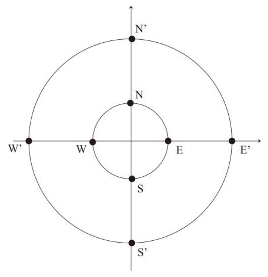
Figure 5.
Schematic diagram of the two groups of the uniform linear array.
The array in the East–West direction includes receiving antennas W, W′, E, E′, where W′ and E′ are virtual antennas and E′E = EW = WW′. The uniform linear array in the North–South direction is the same. Since the four virtual antennas on each uniform linear array are equidistant, the time delay of the received signal of the virtual antenna is easy to obtain. We use the azimuth recognition algorithm to calculate the azimuth of the uniform linear array in the east-west and north-south direction, and then synthesize the two results to get the target azimuth.
Borehole Effect and Correction
The Root-MUSIC algorithm and MUSIC algorithm are only suitable for orientation recognition in homogeneous media. Both borehole and sonde can cause interference to the directional borehole radar azimuth recognition. Therefore, we need to eliminate the borehole effect through the design of the algorithm. We assume that the reflected wave is incident at a certain true azimuth, calculate the time difference between the reflected wave and each receiving antenna, and then calculate the time delay. According to the time delay, we can obtain the apparent azimuth by using the azimuth recognition algorithm in a uniform medium to calculate the azimuth. We can change the true azimuth from 1° to 360°. We can obtain the correspondence between the azimuth and the apparent azimuth, and we can eliminate the borehole effect.
3D Imaging Algorithm
Based on the correction relationship of the non-uniformity around the borehole, we propose and implement the azimuth recognition and 3D imaging algorithm of directional borehole radar under the condition of non-uniformity around the borehole. The algorithm is as follows.
- (1)
- We input relevant parameters, including the receiving and transmitting distances, central frequency of the antenna, relative permittivity of the surrounding rock, relative permittivity of the borehole fluid, relative permittivity of the sonde, time sampling interval, channel spacing, and received signals of the four receiving antennas.
- (2)
- The original data are processed by direct wave.
- (3)
- For each depth, we choose an appropriate window to ensure that the signal of a certain direction in the window is dominant. At the same time, a threshold is selected. When the average value of the four signals in the window is lower than the threshold, the data in the window will be regarded as noise and will not be processed. If it is larger than the threshold, the apparent azimuth is calculated according to the azimuth recognition algorithm in the uniform medium. Move the window, point by point, until all points of the trace are corresponding to this depth point. The above treatment is applied to traces of all depths.
- (4)
- We filter the apparent azimuth to eliminate the burr.
- (5)
- Eliminate borehole effects by using the correspondence between the apparent azimuth and the true azimuth.
- (6)
- For the data of each depth, we use the true azimuth and the original signal to calculate the transverse slice of the depth. The longitudinal slice is obtained by drawing the depth signals of each azimuth in the three-dimensional array.
- (7)
- For each longitudinal slice, migration imaging processing is performed to solve the elevation problem.
- (8)
- Vertical and horizontal slices after migration are used to construct three-dimensional arrays. The first dimension of the three-dimensional array is the number of traces; the second dimension is the azimuth from 0° to 360°. The angle interval is 10°. The third dimension is the number of sampling points. Then, we image the three-dimensional arrays.
3. Results
In this simulation, one transmitting antenna and four receiving antennas are used. Four receiving antennas are located in the South, East, North, and West directions. The main frequency of the antenna is 100 MHz.
3.1. Calculation Results of Two-Dimensional Numerical Simulation
The original waveform of the binary numerical simulation results is shown in Figure 6. We choose the North direction as 0° and the clockwise direction as the positive direction. The azimuth is 24° as shown in Figure 6a. The azimuth is 166° as shown in Figure 6b. The azimuth is 196° as shown in Figure 6c. The azimuth is 329° as shown in Figure 6d. We use the Root-MUSIC algorithm and the MUSIC algorithm to recognize the above waveforms. The angle interval of the MUSIC algorithm is 0.05 degree. We use the corresponding relationship between the apparent azimuth and the true azimuth to remove the influence of the borehole and sonde. The process used a 64-bit computer processor: Intel(R) Core(TM) i5-3230M CPU@ 2.60 GHz, memory 8.0 GB.
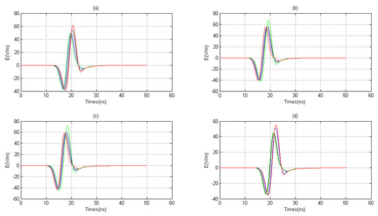
Figure 6.
The received signal waveforms of each azimuth (blue for East-receiving antenna, black for West-receiving antenna, red for North-receiving antenna, green for South-receiving antenna), (a) received signal waveforms of 24° azimuth, (b) received signal waveforms of 166° azimuth, (c) received signal waveforms of 196° azimuth, (d) The received signal waveform is 329° azimuth.
After the calculations, we can obtain the following results:
When the incident wave azimuth of the model is 24 degrees, the azimuth calculated by the Root-MUSIC algorithm is 23.8336 degrees, and the azimuth calculated by the MUSIC algorithm is 23.7159 degrees. The error of the Root-MUSIC algorithm is 0.1664, and the error of the MUSIC algorithm is 0.2841.
When the incident wave azimuth of the model is 166 degrees, the azimuth calculated by the Root-MUSIC algorithm is 166.1731 degrees, and the azimuth calculated by MUSIC algorithm is 166.2133 degrees. The error of the Root-MUSIC algorithm is 0.1731, and the error of the MUSIC algorithm is 0.2133.
When the incident wave azimuth of the model is 196 degrees, the azimuth calculated by the Root-MUSIC algorithm is 196.1932 degrees, and the azimuth calculated by the MUSIC algorithm is 196.2373 degrees. The error of the Root-MUSIC algorithm is 0.1932, and the error of the MUSIC algorithm is 0.2373.
When the incident wave azimuth of the model is 329 degrees, the azimuth calculated by the Root-MUSIC algorithm is 328.8578 degrees, and the azimuth calculated by the MUSIC algorithm is 328.8439 degrees. The error of the Root-MUSIC algorithm is 1422, and the error of the MUSIC algorithm is 0.1561.
Through the above results, we can confirm that the accuracy of the Root-MUSIC algorithm is better than the MUSIC algorithm. This is because the operation error of the Root-MUSIC algorithm mainly comes from the error generated by numerical simulation and the operation error of the MUSIC algorithm not only contains the error generated by numerical simulation, but also contains the error caused by the angle interval in the process of spectrum peak search in the computational space. Therefore, the performance of the Root-MUSIC algorithm is significantly better than that of the MUSIC algorithm.
3.2. Calculation Results of Three-Dimensional Numerical Simulation
For the three-dimensional model, we simulate as follows: the transmitting antenna and the receiving antenna move up from the bottom to the top simultaneously, with the moving step being 0.1 m, with 66 movement increments. The initial depth of the directional borehole radar movement is 8.2 m, and the end depth of the directional borehole radar movement is 1.6 m.
The corresponding synthetic data waveform is shown in Figure 7; this waveform is displayed once every three traces so that the waveform can be seen clearly. It is obvious from the waveform data that the direct wave and the reflected wave came from two targets, and the arrival time of the reflected wave from each antenna is slightly different, which makes directional detection possible.
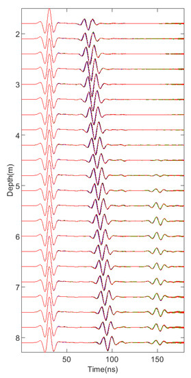
Figure 7.
Signals of four antennas (black: West, green: East, blue: South, red: North).
For the data collected by the borehole radar, the interference components such as the direct wave should be removed first. Then, the MUSIC algorithm and the Root-MUSIC algorithm are used for processing. The angle interval of the MUSIC algorithm is 1 degree. The relationship between the apparent azimuth and the true azimuth is used to remove the borehole effect. Finally, the filtering result is used to filter out the burr caused by the calculation error.
We use the data at the depth of 1.6 m to display. The original waveform data is shown in Figure 8. As seen from Figure 6, the East-receiving antenna receives the signal first, the North-South-receiving antenna receives the signal at the same time, and the West-receiving antenna receives the signal last, which is consistent with the model.
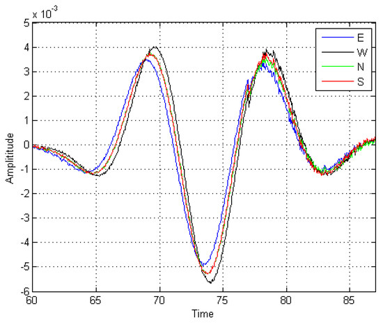
Figure 8.
Raw data of the single-channel waveform at a 1.6 m depth.
We show the spatial spectrum of the MUSIC algorithm at the depth of 1.6 m. The position is at the centre of the window is 68 ns, and the length of the window is 100 sampling points. The spatial spectrum of the MUSIC algorithm is shown in Figure 9, in which the uniform linear array in the East-West direction is 0 in the North-South direction and positive in the East-West direction. As shown in Figure 9a, the azimuth corresponding to the spatial spectrum peak is close to 90°, i.e., due East. The uniform linear array in the North-South direction is 0 in the East-West direction and positive in the South. From Figure 9b, the azimuth corresponding to the peak value of the spatial spectrum is close to 0° in the East-West direction. The azimuth is due East, which is consistent with the model.
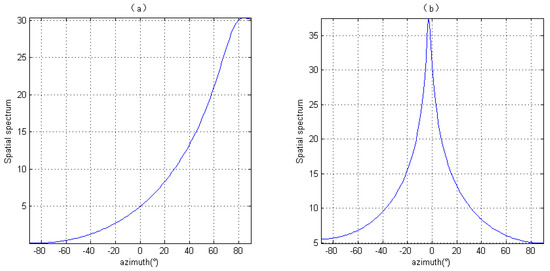
Figure 9.
Spatial spectrum of the MUSIC algorithm, (a) spatial spectrum of the MUSIC algorithm for the East-West uniform linear array, (b) spatial spectrum of the MUSIC algorithm for the North-South uniform linear array.
We calculate the correction relationship between the apparent azimuth and the true azimuth. Because the results of the Root-MUSIC algorithm and the MUSIC algorithm are similar, we choose the results of the Root-MUSIC algorithm to display, as is shown in Figure 10. We use this relationship to remove the influence of the borehole non-uniformity. The result of the orientation recognition is shown in Figure 11. Figure 11a,b are, respectively, the azimuths calculated by the Root-MUSIC algorithm and the MUSIC algorithm. The abscissa of the graph represents the travel time, and the ordinate represents the azimuth. Compared with the model, when the depth is 1.6 m, there is only an inclined crack in the East direction. A signal can be clearly seen in the figure, and the azimuth is approximately 90°, which is in good agreement with the model. As seen from the figure, the accuracy of Figure 11a is significantly higher than that of Figure 11b. The absolute value of the average error of the Root-MUSIC algorithm is 1.6069° and that of the MUSIC algorithm is 2.4711° after calculation.
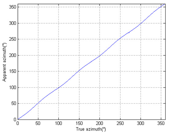
Figure 10.
Correction relationship between the apparent azimuth and the true azimuth.
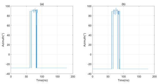
Figure 11.
Orientation recognition results of the first data at 1.6 m depth. (a) Result of the Root-MUSIC algorithm; (b) Result of the MUSIC algorithm.
Using the orientation recognition results, the transverse slice data are synthesized, the 55th trace is selected, and the data are displayed with a depth of 7.1 m, as shown in Figure 12. Figure 12a is the horizontal slice synthesized by the orientation recognition result of the Root-MUSIC algorithm, and Figure 12b is the horizontal slice synthesized by the orientation recognition result of the MUSIC algorithm. According to the model, there is an inclined fracture in the East and a vertical fracture in the South of the borehole. It can be seen from the profile that a signal can be observed in the East and South directions in Figure 12a,b, which is in good agreement with the model. At the same time, the signals in Figure 12a are mainly concentrated in the due South and due East directions, with smaller burrs in other directions, and the effect is stronger than that in Figure 12b. Therefore, the result of the Root-MUSIC algorithm is better than that of the MUSIC algorithm.
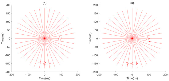
Figure 12.
Orientation recognition results of the first data at 1.6 m depth. (a) Result of the Root-MUSIC algorithm; (b) Result of the MUSIC algorithm.
Based on the orientation recognition results, the longitudinal slice data is synthesized, and the angle interval is selected as 10 degrees. Since the results of the longitudinal slice of the two algorithms have little difference, the longitudinal slice display of the Root-MUSIC algorithm is selected, as shown in Figure 13. From the figure, it can be clearly seen that there is an inclined fracture signal at 90° and a vertical fracture signal at 180° which are in good agreement with the model.
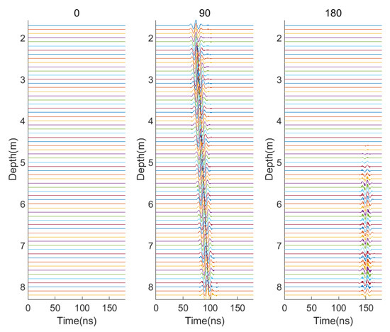
Figure 13.
Longitudinal slices of the Root-MUSIC algorithm.
To solve the problem of the elevation angle, the longitudinal slices in each direction are migrated. The longitudinal slice and the original signal are used to synthesize the three-dimensional array, and the three-dimensional array is filtered and imaged. Because the results of the two algorithms are almost the same, we choose the Root-MUSIC algorithm to display the results, as shown in Figure 14.
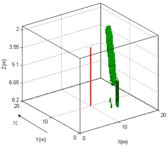
Figure 14.
Three-dimensional imaging of the Root-MUSIC algorithm.
It can be seen from the figure that there is an inclined fracture signal at the depth of 2 m to 8 m in the East direction of the borehole. The top of the inclined fracture signal is approximately 4 m away from the borehole, and the bottom is approximately 5 m away from the borehole. There is a vertical fracture signal at the depth of 6 m to 8 m in the South direction of the borehole, which is approximately 8 m away from the borehole.
4. Discussion
This paper presents and implements a three-dimensional imaging algorithm of the directional borehole radar, based on the Root-MUSIC algorithm. Calculating the roots of polynomials is used to replace the spectral peak search of the MUSIC algorithm so that the accuracy of azimuth recognition is no longer limited by the angle interval of the spectral peak search, which greatly improves the accuracy of azimuth recognition. The results were verified by synthetic data.
The FDTD algorithm is used to synthesize the data. It is verified that the Root-MUSIC algorithm has a significant improvement on the accuracy of the MUSIC algorithm.
For the results of the two-dimensional numerical simulation, we change the position of the transmitting antenna to simulate the performance of the Root-MUSIC algorithm and the MUSIC algorithm in different azimuths. From the results, it can be seen that the azimuth recognition results of the Root-MUSIC algorithm and the MUSIC algorithm are close to the real azimuth, and both methods can carry out effective azimuth recognition. However, the orientation recognition accuracy of the Root-MUSIC algorithm is significantly higher than that of the MUSIC algorithm.
For the results of the three-dimensional numerical simulation, we have the following situation:
For the single-channel waveform at a depth of 1.6 m, the azimuth recognition result is obtained. Both the Root-MUSIC algorithm and the MUSIC algorithm can be used for bearing recognition effectively. Because of avoiding the process of spectral peak searching, the accuracy of the Root-MUSIC algorithm is significantly higher than that of the MUSIC algorithm.
For the horizontal slice, the Root-MUSIC algorithm and the MUSIC algorithm can recognize the azimuth effectively. In the Figure 12, the two algorithms can see obvious signals in the East and South directions. However, the Root-MUSIC algorithm is more focused on energy, and its effect is better than the MUSIC algorithm.
For the longitudinal slice, the azimuth interval is 10°, both the Root-MUSIC algorithm and the MUSIC algorithm can be used for bearing recognition effectively. Both are in good agreement with the model in the display of the longitudinal section. The problem of the elevation angle can be solved by migration imaging. In addition, the three-dimensional imaging results of the two algorithms can see clear targets.
5. Conclusions
The directional borehole radar includes one transmitting antenna and four receiving antennas. Through the arrival sequence of the received waveforms, the accurate azimuth of the target can be determined effectively. In this paper, a target orientation determination algorithm based on the Root-MUSIC algorithm is proposed and implemented. On this basis, a 3D imaging algorithm of the borehole radar is realized. Using the FDTD algorithm synthetic data, the results of the MUSIC algorithm and the Root-MUSIC algorithm are compared. Both can effectively judge the precise orientation of the target, and both have achieved very good results in 3D imaging. At the same time, we find that the Root-MUSIC algorithm is superior to the MUSIC algorithm in its operation accuracy, which is very suitable for directional borehole 3D imaging.
Author Contributions
Conceptualization, methodology, investigation and writing, W.W.; supervision, S.L.; funding support, X.S. and W.Z. All authors have read and agreed to the published version of the manuscript.
Funding
This research was supported by the National key Research and Development Program of China (2017YFC1500103), the Second Tibetan Plateau Scientific Expedition and Research Program (STEP) (2019QZKK0901), National Natural Science Foundation of China (Grant 41874052, 41730212, U1701641 and 41704057), Guangdong Collaborative Innovation Center for Earthquake Prevention and Mitigation (2018B020207011), Guangdong Province Introduced Innovative R&D Team of Deep earth exploration and resource environment (2017ZT07Z066), Guangdong Province Introduced Innovative R&D Team of Geological Processes and Natural Disasters around the South China Sea (2016ZT06N331).
Acknowledgments
The authors thank the school of Geosciences and engineering of Sun Yat sen University for its financial support, the school of earth exploration science and technology of Jilin University for its software support, and the editors and reviewers of remote sensing for their criticism and suggestions on this study.
Conflicts of Interest
The authors declare no conflict of interest.
References
- Jia, Z.; Liu, S.; Zhang, L.; Hu, B.; Zhang, J. Weak Signal Extraction from Lunar Penetrating Radar Channel 1 Data Based on Local Correlation. Electronics 2019, 8, 573. [Google Scholar] [CrossRef]
- Bristow, C.S.; Jol, H.M. Ground Penetrating Radar in Sediments; The Geological Society Publishing House: London, UK, 2003. [Google Scholar]
- Daniels, D.J. Ground Penetrating Radar, 2nd ed.; The Institution of Electrical Engineers: London, UK, 2004. [Google Scholar]
- Jol, H.M. Ground Penetrating Radar: Theory and Applications; Elsevier Science: London, UK, 2009. [Google Scholar]
- Peters, L.; Daniels, J.J. Ground penetrating radar as a subsurface environmental sensing tool. Proc. IEEE 1994, 82, 1802–1822. [Google Scholar] [CrossRef]
- Zhang, L.; Hu, B.; Jia, Z.; Xu, Y. The Subsurface Structure on the CE-3 Landing Site: LPR CH-1 Data Processing by Shearlet Transform. Pure Appl. Geophys. 2020, 177, 3459–3474. [Google Scholar] [CrossRef]
- Sandberg, E.V.; Olsson, O.L.; Falk, L.R. Combined Interpretation of Fracture Zones in Crystalline Rock Using Single-hole, Crosshole Tomography and Directional Borehole-radar Data. Log Anal. Soc. Petrophys. Well-Log Anal. 1991, 32, 108–119. [Google Scholar]
- Liu, S.; Sato, M. Subsurface water-filled fracture detection by borehole radar: A case history. Prog. Geophys. 2004. [Google Scholar] [CrossRef]
- Olsson, O.; Falk, L.; Forslund, O.; Lundmark, L.; Sandberg, E. Borehole radar applied to the characterization of hydraulically conductive fracture zones in crystalline rock. Geophys. Prospect. 1992, 40, 109–142. [Google Scholar] [CrossRef]
- Takayama, T.; Sato, M. A Novel Direction-Finding Algorithm for Directional Borehole Radar. IEEE Trans. Geosci. Remote Sens. 2007, 45, 2520–2528. [Google Scholar] [CrossRef]
- Jang, H.; Kuroda, S.; Kim, H.J. SVD Inversion of Zero-Offset Profiling Data Obtained in the Vadose Zone Using Cross-Borehole Radar. IEEE Trans. Geosci. Remote Sens. 2011, 49, 3849–3855. [Google Scholar] [CrossRef]
- Liu, S.; Sato, M.; Takahashi, K. Application of borehole radar for subsurface physical measurement. J. Geophys. Eng. 2004, 1, 221–227. [Google Scholar] [CrossRef]
- van Dongen, K.W.; van Waard, R.; van der Baan, S.; van den Berg, P.M.; Fokkema, J.T. A Directional Borehole Radar System. Subsurf. Sens. Technol. Appl. 2002, 3, 327–346. [Google Scholar] [CrossRef]
- Ebihara, S.; Wada, K.; Karasawa, S.; Kawata, K. Probe rotation effects on direction of arrival estimation in array-type directional borehole radar. Near Surf. Geophys. 2017, 15, 286–297. [Google Scholar] [CrossRef]
- Liu, L. Fracture Characterization Using Borehole Radar: Numerical Modeling. Water Air Soil Pollut. Focus 2006, 6, 17–34. [Google Scholar] [CrossRef]
- Sato, M.; Tanimoto, T. A shielded loop array antenna for a directional borehole radar. In Proceedings of the Fourth International Conference on Ground Penetrating Radar, Rovaniemi, Finland, 8–13 June 1992. [Google Scholar]
- Lytle, R.J.; Laine, E.F. Design of a Miniature Directional Antenna for Geophysical Probing from Boreholes. IEEE Trans. Geosci. Electron. 1978, 16, 304–307. [Google Scholar] [CrossRef]
- Bradley, J.A.; Wright, D.L. Microprocessor-based data-acquisition system for a borehole radar. IEEE Trans. Geosci. Remote Sens. 1987, 4, 441–447. [Google Scholar] [CrossRef]
- Ebihara, S.; Kimura, Y.; Shimomura, T.; Uchimura, R.; Choshi, H. Coaxial-Fed Circular Dipole Array Antenna with Ferrite Loading for Thin Directional Borehole Radar Sonde. IEEE Trans. Geosci. Remote Sens. 2014, 53, 1842–1854. [Google Scholar] [CrossRef]
- Ebihara, S. Directional borehole radar with dipole antenna array using optical modulators. IEEE Trans. Geosci. Remote Sens. 2004, 42, 45–58. [Google Scholar] [CrossRef]
- Wright, D.L.; Watts, R.D.; Bramsoe, E. A short-pulse electromagnetic transponder for hole-to-hole use. IEEE Trans. Geosci. Remote Sens. 1984, 6, 720–725. [Google Scholar] [CrossRef]
- Ellefsen, K.J.; Wright, D.L. Radiation pattern of a borehole radar antenna. Geophysics 2005, 70, K1–K11. [Google Scholar] [CrossRef]
- Yamada, H.; Ohmiya, M. Superresolution techniques for time-domain measurements with a network analyzer. IEEE Trans. Antennas Propag. 1991, 39, 177–183. [Google Scholar] [CrossRef]
- Yee, K.S. Numerical solution of initial boundary value problems involving maxwell’s equations in isotropic media. IEEE Trans. Antennas Propag. 1966, 14, 302–307. [Google Scholar]
- Abe, T.; Sato, M. A cavity measurement by polarimetric borehole radar and a verification by FDTD. Tech. Rep. Ieice Sane 2001, 101, 57–64. [Google Scholar]
- Zivanovic, S.S.; Yee, K.S. A subgridding method for the time-domain finite-difference method to solve Maxwell’s equations. IEEE Trans. Microw. Theory Tech. 1991, 39, 471–479. [Google Scholar] [CrossRef]
- Chevalier, M.W.; Luebbers, R.J.; Cable, V.P. FDTD local grid with material traverse. IEEE Trans. Antennas Propag. 1997, 45, 411–421. [Google Scholar] [CrossRef]
- Sun, S.H.; Choi, C. A new subgridding scheme for two-dimensional FDTD and FDTD (2,4) methods. IEEE Trans. Magn. 2004, 40, 1041–1044. [Google Scholar] [CrossRef]
- Monk, P. Sub-gridding FDTD schemes. Appl. Comput. Electromagn. Soc. J. 1996, 11, 37–46. [Google Scholar]
- Chen, J.; Zhang, A. A Subgridding Scheme Based on the FDTD Method and HIE-FDTD Method. Appl. Comput. Electromagn. Soc. J. 2011, 26, 1. [Google Scholar]
- Huang, Y.J.; Wang, Y.W.; Meng, F.J.; Wang, G.L. A spatial spectrum estimation algorithm based on adaptive beamforming nulling. In Proceedings of the 2013 Fourth International Conference on Intelligent Control and Information Processing (ICICIP), Beijing, China, 9–11 June 2013. [Google Scholar]
- Schmidt, R.; Schmidt, R.O. Multiple emitter location and signal parameter estimation. IEEE Trans. Antennas Propag. 1986, 34, 276–280. [Google Scholar] [CrossRef]
- Krim, B.H.; Viberg, M. Two decades of array signal processing research. IEEE Signal Process. Mag. 1996, 13, 67–94. [Google Scholar] [CrossRef]
- Ebihara, S.; Sato, M.; Niitsuma, H. Super-resolution of coherent targets by a directional borehole radar. IEEE Trans. Geosci. Remote Sens. 2000, 38, 1725–1732. [Google Scholar] [CrossRef][Green Version]
Publisher’s Note: MDPI stays neutral with regard to jurisdictional claims in published maps and institutional affiliations. |
© 2021 by the authors. Licensee MDPI, Basel, Switzerland. This article is an open access article distributed under the terms and conditions of the Creative Commons Attribution (CC BY) license (https://creativecommons.org/licenses/by/4.0/).