Sinkhole Scanner: A New Method to Detect Sinkhole-Related Spatio-Temporal Patterns in InSAR Deformation Time Series

Abstract

Sinkholes are sudden disasters that are usually small in size and occur at unexpected locations. They may cause serious damage to life and property. Sinkhole-prone areas can be monitored using Interferometric Synthetic Aperture Radar (InSAR) time series. Defining a pattern using InSAR-derived spatio-temporal deformations, this study presents a sinkhole pattern detector, called the Sinkhole Scanner. The Sinkhole Scanner includes a spatio-temporal mathematical model such as a 2-dimensional time evolving Gaussian function as a kernel, which moves over the study area using a sliding window approach. The scanner attempts to fit the model over deformation time series of Constantly Coherent Scatterers (CCS) intersected by the window and returns the posterior variance as a measure of goodness of fit. In this way, the scanner searches for subsiding regions resembling sinkhole shapes over a sinkhole prone area. It is designed to detect large sinkholes with a high efficiency, and small sinkholes with a lower efficiency. It is tested at four different spatial scales, and on a simulated and real set of deformation data. Real data were obtained from Sentinel-1A SLC data in IW mode, over Ireland where a large sinkhole occurred on 24 September 2018. The Sinkhole Scanner was able to identify a pattern of low posterior variance zones consistent with the simulated set. In case of the real data, it is able to identify significantly low posterior variance zones near the sinkhole area with the lowest value being 51.1% of the maximum value. The results from Sinkhole Scanner over the real sinkhole site were compared with Multiple Hypothesis Testing (MHT), which identifies Breakpoint and Heaviside temporal anomalies in the deformation time series of CCS. MHT was able to identify high likelihood for Heaviside anomalies in deformation time series of CCS near the sinkhole site about 10 epochs before the sinkhole occurrence. We show that the Sinkhole Scanner is efficient in monitoring a large area and search for sinkholes and that MHT can be used successively to identify temporal anomalies in the vicinity of areas detected by the Sinkhole Scanner. Future research may address other Sinkhole shapes whereas the underlying stochastic model may be adjusted. We conclude that the Sinkhole Scanner is important to be applied at different levels of scale to converge on potential sinkhole centers.

1. Introduction

The surface of the Earth is in a state of dynamic equilibrium due to a range of geophysical and geochemical phenomena. A particular phenomenon that we study in this paper concerns cavities that are formed due to the dissolution of subsurface bedrock, see Figure 1a. They result in unbalanced gravitational forces due to the Earth mass present above the cavity [1]. The burden of mass gradually sinks into the cavity and thereby leads to subsidence. Regularly, this gradual subsidence manifests itself on the ground surface [2]. This phenomenon is defined as a sinkhole. Sinkholes commonly but not exclusively occur in karst terrains [3]. Subsidence of the top surface varies in shape and size depending upon the soil type and nature of cavity formed underneath [4].

Sinkholes may exhibit precursory subsidence, indicating their formation. Early detection of precursory deformation patterns is important for early warning and sinkhole monitoring [2]. Sinkholes can be monitored using both in situ and remote sensing methods. For instance, leveling [5], extensometers [6] are helpful to monitor micrometer scale deformations in mining galleries, and micro-seismics are used to monitor activity in salt mining caverns [7]. Passive optical [8] and thermal remote sensing using UAVs [9] is used to monitor sinkhole prone regions. However, these methods have limited coverage and are expensive when monitoring large areas. Radar remote sensing using instruments such as Synthetic Aperture Radar (SAR) [10], can be useful to do so at a relatively lower cost. SAR images have a large spatial coverage, a high spatio-temporal resolution, and data from few sensors can be freely accessed like for Sentinel-1 SAR [11]. In the past three decades, conventional InSAR (Interferometric SAR) and time series InSAR (TSInSAR) techniques have been successfully applied to land subsidence monitoring [12,13,14,15,16,17]. TSInSAR is particularly well established in monitoring post-hazard surface deformation patterns [14], but it is only partially developed for observing small spatial scale hazards such as sinkholes [2,18,19]. Moreover, there is a lack of generic methods to detect sinkholes, although attempts have been made to model TSInSAR derived deformations as Gaussian shaped sinkholes [20].

Detection of sinkhole-related precursory deformation patterns can be conducted by either modeling the deformation patterns using known deformation models, e.g., Gaussian subsidence bowl, or by identifying anomalies in InSAR deformation time series. Modeling deformation patterns works well in detecting subsidence in a region of a high Constantly Coherent Scatterer (CCS) density, while identifying anomalies in InSAR deformation time series is recommended if the CCS spatial density is relatively low. Application and efficacy of the methods depend upon the CCS density in the sinkhole area of interest. The CCS density is commonly limited by the spatial and temporal decorrelation and atmosphere heterogeneity, especially in rural areas. Simulation of synthetic sinkholes can thus help in further developing models to detect sinkholes, based upon contextual information. Sinkhole simulations have been conducted by simulating subsurface bedrock and interaction between bedrock particles [1] during the occurrence of a cavity. When the cavity migrates upwards, surface deformation manifests itself on the surface, which could be modeled as a spherical Gaussian function. Modeling of surface deformation due to sinkholes has been done as well using viscoelastic modeling [21]. Currently, SAR-based sinkhole monitoring methods vary with respect to the spatial and temporal resolution of the images. Various SAR satellites provide data at different spatio-temporal resolutions and in different modes. The spatial resolution of currently available SAR products ranges between high (e.g., TerraSAR-X Stripmap mode) to medium (e.g., Sentinel-1 IW mode). High-resolution images allow us to identify the formation of sinkhole-related patterns using interferograms [19]. They are based on Gaussian-shaped patterns that, however, are unlikely to appear on medium resolution images. Sentinel-1A&B [11] offer medium spatial resolution SAR data with resolution equal to 20 m × 5 m in azimuth and slant range directions and a relatively high temporal resolution of up to six days. To study sinkholes, medium resolution Sentinel-1 data [22], unwrapped interferograms, and time series InSAR methods [18,23] have been used. Sinkholes have mainly been studied by analyzing deformation trends over constantly coherent scatterers (CCS) such as persistent scatterers (PS), detecting anomalous behaviour in InSAR deformation time series. Sinkhole-related subsidence can also be studied by searching for instantaneous acceleration or non-steady-state deformation behavior. Such behavior can manifest as a Heaviside anomaly [24] in a deformation time series. Moreover, deformation behaviour can also manifest itself as a change in the linear deformation velocity model, where the deformation velocity increases a few epochs before the sinkhole occurrence [18]. This is termed as a Breakpoint anomaly. Such anomalies have been modeled using the Multiple Hypothesis Testing (MHT) [25].

The main objective of this study is to design and test a sinkhole detection method called the Sinkhole Scanner. It is based upon modeling the deformation time series, derived from InSAR, as spatio-temporal deformation patterns, using the inverted Gaussian function. The Sinkhole Scanner is designed on the basis of a spatio-temporal deformation model and using a moving window, inside which the deformation time series is modeled. The Sinkhole Scanner is mainly tested by detecting sinkhole related spatio-temporal deformation patterns over simulated and real sinkholes. Furthermore, the test results from this Sinkhole Scanner method are compared with the results from the Multiple Hypothesis Testing.

The remainder of the paper is arranged as follows. Section 2 presents a brief background on various sinkhole shapes and relates them to bedrock properties. Section 3 introduces the method for TSInSAR, sinkhole simulation, Sinkhole Scanner, moving window operation, and MHT. Section 4 presents the details of the study area and Sentinel-1 data used. Section 5 states the results followed by a discussion in Section 6. Finally, Section 7 draws conclusions and also gives future recommendations.

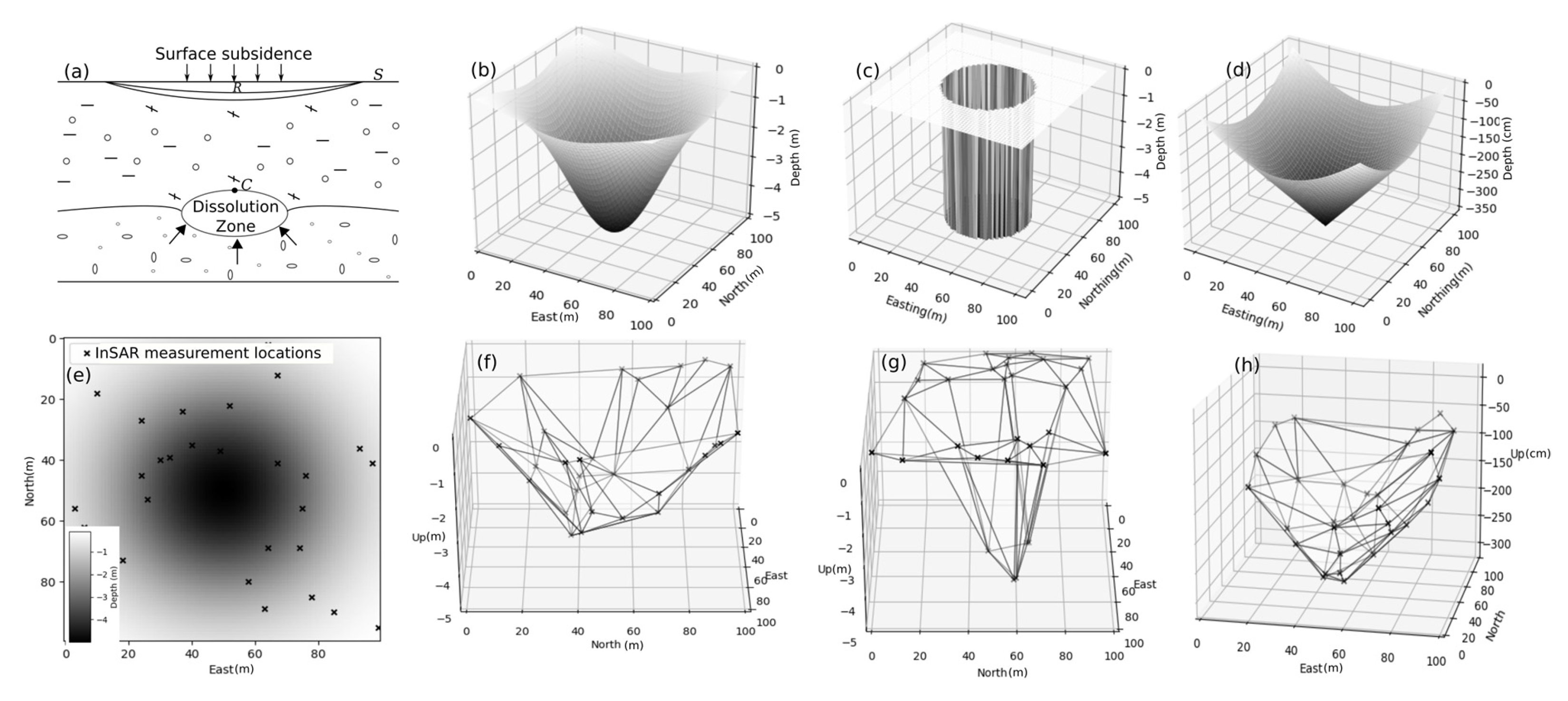
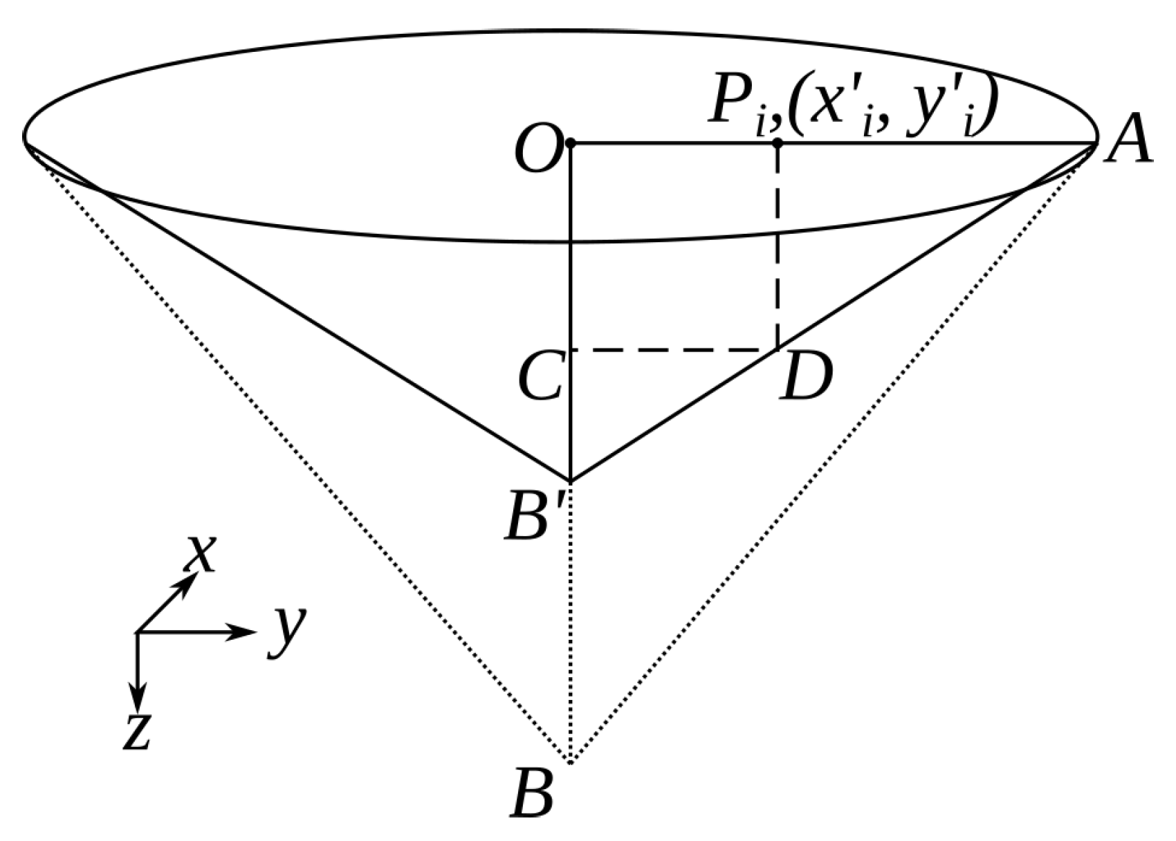
2. Background on Sinkhole Types and Shapes

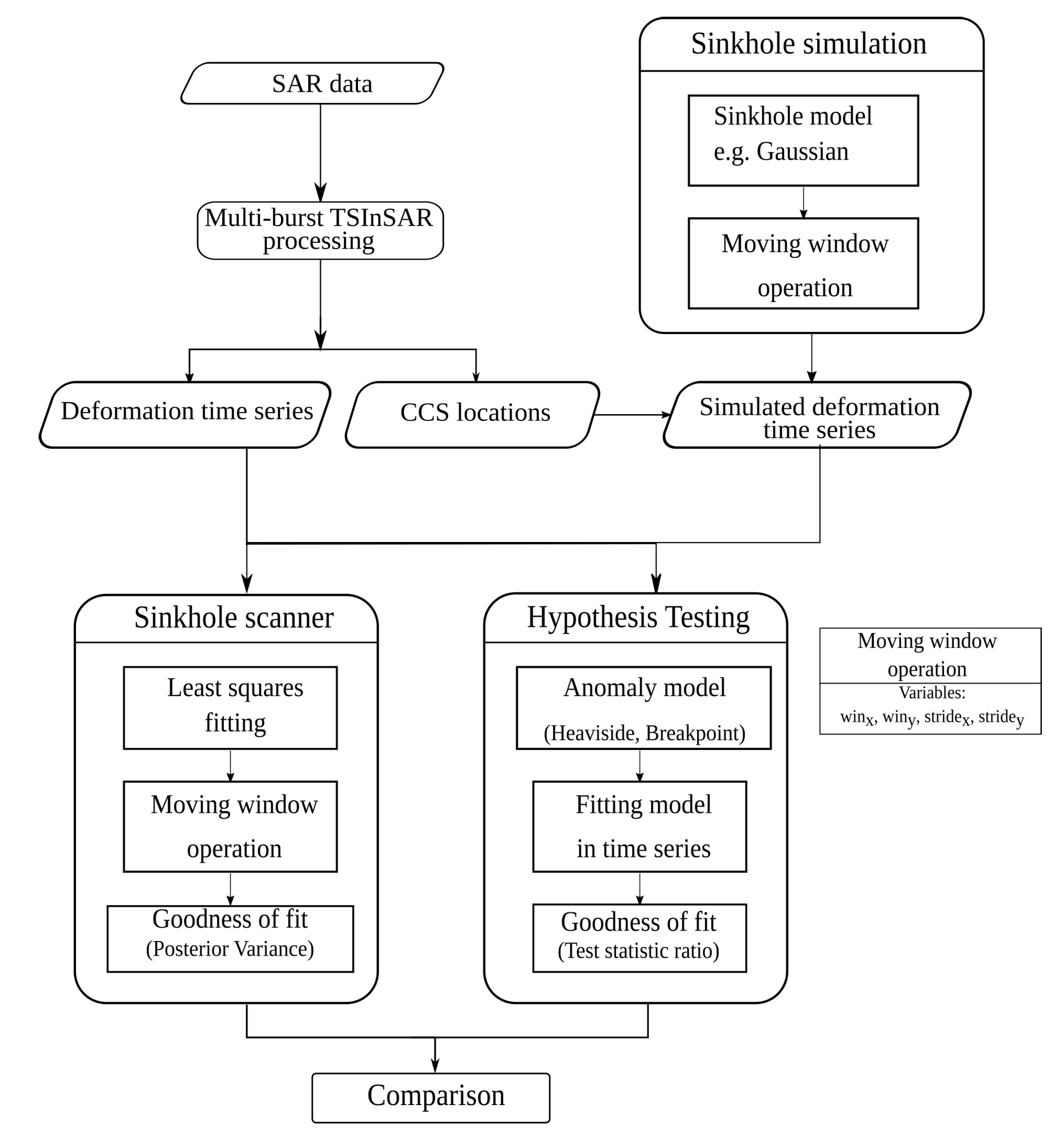
The diameter of sinkholes commonly ranges between 1 and 300 m [4], while their evolution depends upon the nature of the terrain and the mechanism of material loss in the region. Usually, sinkholes have a low depth to diameter ratio if they occur over materials which have weaker cohesion, while they have a high depth to diameter ratio if the material has high cohesion [1]. Following the authors of [4], we distinguish four major categories of sinkholes or dolines: Dissolution, Collapse, Dropout, and Suffosion dolines. Dissolution dolines occur by water penetration through a large number of small fissures, followed by dissolving the rocks solutes. This is followed by a collapse caused by weathering of the overburden material [26]. Their shape is often Gaussian, see an example shown in Figure 1b, and the subsidence on the surface is gradual and evident. Collapse dolines occur when the above ground suddenly collapses into the cavity created below. This generally results in a cylindrical or steep sided conical shape. These types of sinkholes occur generally in karst and volcanic regions [27]. An example is shown in Figure 1c. Dropout or subsidence dolines occur majorly in urban areas and are relatively small in size, such as $10\mathrm{m}$ in diameter. These sinkholes are quite dangerous because they cause sudden failure of the ground. Suffosion dolines are caused through constant loss of underground material through a channel. This results in a funnel-shaped structure. An example is shown in Figure 1d. From the above, we note that the most common shapes of sinkholes are inverted Gaussian, cylinders, and cones.

Figure 1e shows an example of a random distribution of 30 CCS which can be used to reconstruct the formation of a sinkhole shapes, as shown in Figure 1f–h for cylindrical, cylindrical, and conical shapes, respectively. In this study, we will use this way of reconstructing sinkhole shapes from TSInSAR-derived CCS location and their corresponding deformation time series.

3. Methods

This part first reviews the method for CCS location and associated deformation time series extraction using multi-burst SAR data in Section 3.1. It next describes the sinkhole simulation method and its use in extracting simulated sinkhole-related deformation time series in Section 3.2. It then presents the sinkhole scanner method in Section 3.3, and the method for moving window operation in Section 3.4. The MHT method [25] used for detecting temporal anomalies in individual deformation time series of CCS points is discussed in Section 3.5.

3.1. Multi-Burst TSInSAR Processing

An overview of the used methods can be seen in Figure 2. Given a stack of SAR images (usually $\ge 20$), a standard TSInSAR processing can be applied to obtain the location of the CCS and their corresponding deformation time series in the line of sight (LOS) direction. Every Sentinel-1 SAR image in Interferometric Wide (IW) swath mode contains three sub-swath images, and each sub-swath image consists of nine bursts with sufficient overlap between adjacent bursts [28]. When the study area covers multiple bursts/swaths, multi-burst TSInSAR processing is required.

Here, we take two-burst TSInSAR processing as an example and employ the Delft implementation of Persistent Scatterer InSAR (DePSI) as one of the tool packages for PSI processing [29,30,31]. For single-master interferogram stack generation, we first deramp all Sentinel-1A SAR images for each burst to improve the coregistration [28] and next coregister all slave images with the master image using Sentinel-1 precise orbit data and Digital Elevation Model (DEM)-Assisted Coregistration (DAC). Then, we reramp all images and create the interferogram stack by multiplying the complex conjugates of all slave images with the master image [32]. To concatenate bursts in a same swath, we use the deburst method presented in [33]. In this method, the bursts are concatenated using the average burst scan time in azimuth direction and scan time per azimuth line [34]. Specifically, the merging time $t_{\mathrm{merg}}$ of two adjacent bursts can be calculated by $t_{\mathrm{merg}}=(t_{zd,be}^{\mathrm{last}}+t_{zd,bl}^{\mathrm{first}})/2$. Here, $t_{zd,be}^{\mathrm{last}}$ and $t_{zd,bl}^{\mathrm{first}}$ represent the zero Doppler time ($zd$) for the last line of the earlier burst ($be$), and first line of the latter burst ($bl$), respectively. After debursting, PSI processing with, e.g., DePSI can be conducted as DePSI tool is customized to spatially divide debursted interferograms into small patches for efficient PSI processing in a large area.

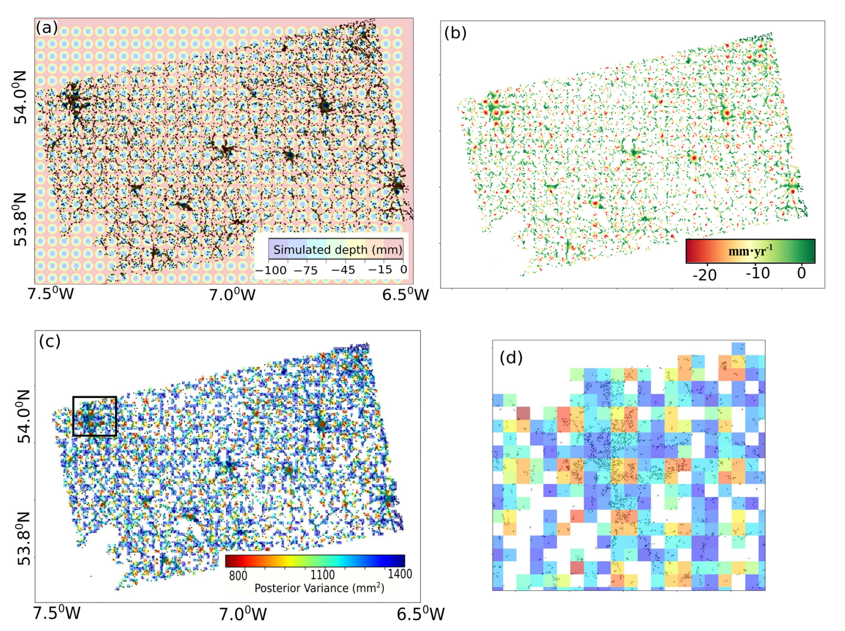
3.2. Sinkhole Simulation

As discussed in Section 2, three sinkhole models are used in sinkhole simulation and later in modeling the data. The definitions of the sinkholes shapes are described in

Table 1. Sinkhole inventory: mathematical model of shapes used for sinkhole modeling.

	Inverted Gaussian Model	Cylindrical Model	Conical Model
Model equation	$F(x,y,t)=$$I\left(t\right)·e^{-\left(\frac{x^2+y^2}{2·{\zeta }^2}\right)}$	$F\left(t\right)=I\left(t\right)$, $\forall P_i\mid {x_i^{\prime }}^2+{y_i^{\prime }}^2\le r^2$	$F(x,y,t)=I\left(t\right)\left(1-\frac{\sqrt{(x^2+y^2)}}{r}\right)$$\forall P_i\mid {x_i^{\prime }}^2+{y_i^{\prime }}^2\le r^2$
Model parameters	$\zeta ,v$	$v,c$	$v,c$

r: radius of extent for the cylindrical and conical function on the top surface, $P_i$: $i^{th}$ CCS with coordinates ($x_i^{\prime },y_i^{\prime }$), relative to the center of the sinkhole ($x_0,y_0$), $I\left(t\right)=v·t+c$, t: time step, v: linear velocity rate, c: constant term, and $\zeta$ signifies the extent of the Gaussian function.

. The deformation function F is defined as a function of the two-dimensional coordinates ($x,y$) over the ground surface, and time t. Therefore, each function has a spatial and a temporal component. In time, the sinkhole shape can be assumed to evolve linearly, and is defined as $I\left(t\right)=v·t+c$, where v is the linear deformation velocity of the center of sinkhole model located at ($x_0,y_0$), and c is the constant term. In space, the sinkholes are defined on the 2-D horizontal surface using the functions described in Table 1. The deformation functions F for Gaussian and Conical models are dependent upon spatial coordinates ($x,y$), whereas the deformation function for the Cylindrical model is independent of the spatial coordinates, and models the subsidence of points using the temporal model only. For the Cylindrical and Conical functions, there is a constraint placed on the points: $\forall P_i\mid {x_i^{\prime }}^2+{y_i^{\prime }}^2\le r^2$, where $P_i$ represents CCS points with $i\in [1,b]$, ($x_i^{\prime },y_i^{\prime }$) represents the CCS coordinates relative to the center of the sinkhole, r is the radius of extent for the cylindrical and conical function on the top surface, and b is the total number of CCS intersected in the simulation window. Therefore, this means that only the points located within the circle with radius r and sinkhole center ($x_0,y_0$) are influenced by the simulated deformation function F, and later, participate in the inverse modeling of sinkholes, see Section 3.3.

The assumptions behind these simulations are that the sinkhole evolves in the shape of one of the sinkhole models defined in the sinkhole inventory, and that the radar signal is able to capture the movement of surface at the location of CCS, albeit in the LOS direction. Synthetic deformation time series is simulated over the estimated CCS locations. The deformation time series of the CCS locations, modulated with artificial Gaussian noise is obtained by

$${\underline{d}}_{P_i}\left(t\right)=F(x_{P_i},y_{P_i},t)+d_e;d_e\sim \mathcal{N}(0,{\sigma }^2),$$

(1)

where ${\underline{d}}_{P_i}\left(t\right)$ is the deformation at the CCS locations $\forall P_i,i\in [1,b]$, which is extracted from the simulated deformation function F; b is the total number of CCS; and $\mathcal{N}(0,{\sigma }^2)$ signifies a normally distributed noise with zero expectation and $\sigma$ standard deviation introduced to simulate the error $d_e$ in the deformation. The sinkhole is then positioned over a location in the study area using the moving window operation.

3.3. Sinkhole Scanner

The Sinkhole Scanner is defined as a two-dimensional testing space shaped by its window size in the $x-y$ plane and the scanning operator. The scanner moves in either directions over the observation space with a predefined stride in the x and y directions. The testing window searches for sinkhole shapes defined in the sinkhole inventory that show an evolving pattern. For instance, for the Gaussian shape this is obtained by solving the mathematical model of the sinkhole shape, e.g., Equation (4) for Inverted Gaussian shape. The following text describes the mathematical models for the three sinkhole models derived using the deformation functions F, defined in Table 1.

Inverted Gaussian shape solution:

As the inverted Gaussian model is described as a nonlinear equation in Table 1, the least squares estimation cannot be employed in a straightforward way. Therefore, we linearize this nonlinear equation to have its linear form, by using the logarithmic transformation,

$$log(F(x,y,t)/t)=-\left(\frac{x^2+y^2}{2·{\zeta }^2}\right)+log\left(v\right).$$

(2)

Upon this, we can define the corresponding functional and stochastic model, expressed as [35]

$$E\left\{\underline{\mathit{d}}\right\}=\mathbf{A}·\mathbf{x};D\left\{\underline{\mathit{d}}\right\}=Q_{\mathit{dd}},$$

(3)

where $E\left\{\right\}$ and $D\left\{\right\}$ are the expectation operator and dispersion operator. The matrix A is the design matrix and x is the vector of unknowns. The stochastic model $Q_{\mathit{dd}}$ is designed to describe the observation errors. By relating the functional model in Equation (3) with Equation (2), we specify the functional model of the inverted Gaussian model as

$$E\left\{\underline{\mathit{d}}\right\}=E\{\underset{\underline{\mathit{d}}}{\underbrace{\left[\begin{array}{c}log(\underline{\mathit{d}}(x_1,y_1,t_1+\delta )/t_1)\\ log(\underline{\mathit{d}}(x_1,y_1,t_2+\delta )/t_2)\\ ⋮\\ log(\underline{\mathit{d}}(x_1,y_1,t_m+\delta )/t_m)\\ log(\underline{\mathit{d}}(x_2,y_2,t_1+\delta )/t_1)\\ ⋮\\ log(\underline{\mathit{d}}(x_b,y_b,t_{m-1}+\delta )/t_{m-1})\\ log(\underline{\mathit{d}}(x_b,y_b,t_m+\delta )/t_m)\end{array}\right]}}\}=\underset{\mathbf{A}}{\underbrace{\left[\begin{array}{cc}-(x_1^2+y_1^2)/2& 1\\ -(x_1^2+y_1^2)/2& 1\\ ⋮\\ -(x_1^2+y_1^2)/2& 1\\ -(x_2^2+y_2^2)/2& 1\\ ⋮\\ -(x_b^2+y_b^2)/2& 1\\ -(x_b^2+y_b^2)/2& 1\end{array}\right]}}\underset{\mathbf{x}}{\underbrace{\left[\begin{array}{c}{\zeta }^{-2}\\ log\left(v\right)\end{array}\right]}}.$$

(4)

The vector $\underset{bm\times 1}{\underline{\mathit{d}}}$ comprises of the logarithmic transform of deformation obtained over b points that are overlapped by the testing window, with m epochs. The b points are CCS located at $(x_i,y_i),\forall i\in [1,b]$. The deformation in the observation space are given an offset by a common factor $\delta =\min \left(\underline{\mathit{d}}(x_i,y_i,t_j)\right);i\in [1,b],j\in [1,m]$, so as to avoid negative values in the argument of the log function. This factor is chosen to be the deepest deformation estimate with the addition of a small positive real number such that all deformation values are non-zero and positive real numbers. The design matrix A and the unknown parameters x have the size of $bm\times 2$ and $2\times 1$, respectively. The estimates of the extent of the Gaussian function $\widehat{\zeta }$ and the linear velocity $\widehat{v}$ can be determined once $\widehat{\mathbf{x}}$ is estimated. The corresponding stochastic model $\underset{bm\times bm}{Q_{\mathit{dd}}}$ describes the deformation errors in logarithmic form. To simplify the simulation, one can use a scaled identity matrix, i.e., $Q_{\mathit{dd}}={\sigma }^2·R_{bm\times bm}={\sigma }^2·{\mathbb{I}}_{bm\times bm}$, which implies deformation of the b points are uncorrelated in time and space and the deformation variance is invariant over time. Here, ${\sigma }^2$ is the variance of unit weight, $R_{bm\times bm}$ is the cofactor matrix, and ${\mathbb{I}}_{bm\times bm}$ is the identity matrix.

Cylinder shape solution:

The cylindrical and conical function are dependent upon the user defined parameter for the extent of the sinkhole r. The default value for this variable is chosen to be half of the scanner window size. The solution for the cylindrical sinkholes is performed by firstly applying the constraint $\forall P_i\mid {x_i^{\prime }}^2+{y_i^{\prime }}^2<r^2$. The CCS inside the circle centered at the center of the scanning window and with radius r are modeled using a common linear deformation velocity, expressed as (see in Table 1 as well)

$$F\left(t\right)=I\left(t\right)=v·t+c,$$

(5)

where v and c represent the linear deformation velocity and the constant term in the model fitting, respectively. The CCS outside the circle, but inside the scanning window, are assumed to be in a steady state. Assuming $b^{\prime }$ points are intersected due to the constraint, the functional model and stochastic model shown in Equation (3), with b replaced by $b^{\prime }$, can be used to solve for the cylinder shape. Specifically, in this case the functional model can be expressed as

$$E\left\{\underline{\mathit{d}}\right\}=E\{\underset{\underline{\mathit{d}}}{\underbrace{\left[\begin{array}{c}\underline{\mathit{d}}(x_1,y_1,t_1)\\ \underline{\mathit{d}}(x_1,y_1,t_2)\\ ⋮\\ \underline{\mathit{d}}(x_1,y_1,t_m)\\ \underline{\mathit{d}}(x_2,y_2,t_1)\\ ⋮\\ \underline{\mathit{d}}(x_{b^{\prime }},y_{b^{\prime }},t_{m-1})\\ \underline{\mathit{d}}(x_{b^{\prime }},y_{b^{\prime }},t_m)\end{array}\right]}}\}=\underset{\mathbf{A}}{\underbrace{\left[\begin{array}{cc}{t}_1& 1\\ t_2& 1\\ ⋮\\ t_m& 1\\ t_1& 1\\ ⋮\\ t_{m-1}& 1\\ t_m& 1\end{array}\right]}}\underset{\mathbf{x}}{\underbrace{\left[\begin{array}{c}v\\ c\end{array}\right]}},$$

(6)

where $\underset{b^{\prime }m\times 1}{\underline{\mathit{d}}}$ represents the deformation observation vector. The matrix A, with size $b^{\prime }m\times 2$ is the design matrix and x, with size $2\times 1$ is the vector of unknowns.

Conical shape definition:

Similar to the solution for cylindrical shape, the points satisfying $\forall P_i\mid {x_i^{\prime }}^2+{y_i^{\prime }}^2<r^2$, are used for solving the model equation. The functional model is derived using Figure 3, where $▵B^{\prime }CD\sim ▵B^{\prime }OA,\therefore CD/OA=B^{\prime }C/B^{\prime }O$. $CD=O{P}_i=\sqrt{{x_i^{\prime }}^2+{y_i^{\prime }}^2},OA=r,B^{\prime }O=v·t^{\prime }+c$, see Figure 3. Therefore, the observation function of any point $P_i$ can be written as

$${\underline{\mathit{d}}}_{P_i}^{t^{\prime }}=t^{\prime }\left(1-\frac{\sqrt{{x_i^{\prime }}^2+{y_i^{\prime }}^2}}{r}\right)·v+\left(1-\frac{\sqrt{{x_i^{\prime }}^2+{y_i^{\prime }}^2}}{r}\right)·c.$$

(7)

Here, the unknown parameters are the velocity of sinkhole center is denoted by v and the constant term associated to the model is denoted by c. The corresponding functional model is described as

$$E\left\{\underline{\mathit{d}}\right\}=E\{\underset{\underline{\mathit{d}}}{\underbrace{\left[\begin{array}{c}\underline{\mathit{d}}(x_1,y_1,t_1)\\ \underline{\mathit{d}}(x_1,y_1,t_2)\\ ⋮\\ \underline{\mathit{d}}(x_1,y_1,t_m)\\ \underline{\mathit{d}}(x_2,y_2,t_1)\\ ⋮\\ \underline{\mathit{d}}(x_{b^{\prime }},y_{b^{\prime }},t_{m-1})\\ \underline{\mathit{d}}(x_{b^{\prime }},y_{b^{\prime }},t_m)\end{array}\right]}}\}=\underset{\mathbf{A}}{\underbrace{\left(1-\frac{\sqrt{{x_i^{\prime }}^2+{y_i^{\prime }}^2}}{r}\right)\left[\begin{array}{cc}{t}_1& 1\\ t_2& 1\\ ⋮\\ t_m& 1\\ t_1& 1\\ ⋮\\ t_{m-1}& 1\\ t_m& 1\end{array}\right]}}\underset{\mathbf{x}}{\underbrace{\left[\begin{array}{c}v\\ c\end{array}\right]}}.$$

(8)

Here, $\underline{\mathit{d}}$ has the size of $b^{\prime }m\times 1$, where $b^{\prime }$ signifies the number of points intersected by the constraint circle. The symbols have the same meaning as in the case of Cylindrical model. Moreover, the shapes of A and x are the same as in the previous Cylinder shape case as well.

According to the least squares estimation method, the unknown parameters of the mathematical models shown in Equation (3), are estimated by

$$\widehat{\mathbf{x}}={\left({\mathbf{A}}^T{Q}_{\mathit{dd}}^{-1}\mathbf{A}\right)}^{-1}{\mathbf{A}}^T{Q}_{\mathit{dd}}^{-1}\underline{\mathit{d}}.$$

(9)

The error after the parameter estimation is obtained as $\widehat{\underline{\mathit{e}}}=\underline{\mathit{d}}-A·\widehat{\mathbf{x}}$. The precision of the least-squares estimations can be estimated by $Q_{\widehat{e}\widehat{e}}=Q_{\mathit{dd}}-A{\left(A^T{Q}_{\mathit{dd}}^{-1}A\right)}^{-1}{A}^T$.

The detectability of the model is assessed using root mean square error RMSE = $\sqrt{E[{\widehat{e}}^2]}$, and posterior variance ${\widehat{e}}^T{(Q_{\mathit{dd}}/{\sigma }^2)}^{-1}\widehat{e}/(bm-n)$ for inverted Gaussian shape, ${\widehat{e}}^T{(Q_{\mathit{dd}}/{\sigma }^2)}^{-1}\widehat{e}/(b^{\prime }m-n)$ for conical and cylindrical shapes, after fitting the model to the data. Here, n is the number of unknown parameters, i.e., 2, and ${\sigma }^2$ is the variance of unit weight.

3.4. Moving Window Operation

Instead of moving the scanner over the whole study area, and intersecting points with the moving window, we suggest to efficiently identify sinkhole scanning locations based upon the locations of CCS points. We identify the lower-left coordinate of the box encompassing the CCS points in the area by

$${\mathrm{Box}}^{ax,0}=⌊\frac{P_i^{ax}-\min \left(P_i^{ax}\right)}{{\mathrm{win}}^{ax}}⌋·{\mathrm{win}}^{ax}+\min \left(P_i^{ax}\right),$$

(10)

where ${\mathrm{Box}}^{ax,0}$ represents the initial position of the window or box on axis $ax,ax\in \{x,y\}$, and the superscript 0 identifies the bottom left index of the window. The parameter $P_i^{ax}$ represents the component of the positional vector of $P_i$ of the $i^{th}$ CCS point with $i\in [1,b]$ on the axis $ax$, and ${\mathrm{win}}^{ax}$ represents the window size on the corresponding axis. The notation $\lfloor .\rfloor$ represents the greatest integer function and $\min \left(\right)$ is the minimum operator.

Unique windows are identified using Equation (10). The corresponding CCS point locations and deformation estimates are grouped with the boxes, as attributes of the box. The Scanner then performs an iteration over the boxes and their grouped attributes by performing a least squares estimation. This one-dimensional iteration method largely enhances the performance of the Scanner as compared to two-dimensional iterations with successive intersection of CCS points with the moving windows.

3.5. Hypothesis Testing Method

The pointwise hypothesis testing is used to identify anomalies in time. The Breakpoint [18] and Heaviside anomalies [24] are chosen to be two temporal anomalies which can resemble sinkhole-related deformation behaviour. Hypothesis testing is used to identify the best epochs in the deformation time series where either a Heaviside model, or a Breakpoint model, with one jump, or break, would fit. The functions for Heaviside ($M_H\left(\right)$) and Breakpoint anomalies $M_{Br}\left(\right)$ are defined as [25]

$$M_H\left({\Delta }_i\left(P_k\right)\right)={\Delta }_i\left(P_k\right)\mathcal{H}(t-{\tau }_i\left(P_k\right)),i\in [1,m],k\in [1,b];$$

(11)

$$\begin{array}{cc}\hfill M_{Br}^k\left(v_k\right)& =t_k·v_k;k\in [1,m].\hfill \end{array}$$

(12)

Here, $\mathcal{H}(t-{\tau }_i\left(P_k\right))$, for $i\in [1,m-1]$ is the Heaviside step function, centered at ${\tau }_i\left(P_k\right)$, ${\Delta }_i\left(P_k\right)$ is the Heaviside step size, $v_k$ is the deformation velocity at time $t_k$. For instance, for a single Breakpoint model, the deformation time series is divided into two parts with two different linear velocity parameters, i.e., $v_1$ and $v_2$, at the breakpoint epoch l. The corresponding single Breakpoint model can be written as $M_{Br}^i\left(v_1\right)=t_i·v_1,i\in [1,l],M_{Br}^i\left(v_2\right)=t_i·v_2,i\in [l+1,m]$.

This anomaly detection is done by calculating the test statistic and test statistic ratios for a null hypothesis and other alternative hypotheses (details in Section II in [25]). The null hypothesis $H_0$ and alternative hypotheses $H_j$, for instance, for the inverted Gaussian shaped sinkhole case, can be expressed as [25]

$$\begin{array}{cc}\hfill H_0& :E\underset{bm\times 1}{\left\{\underline{\mathit{d}}\right\}}=\underset{bm\times n}{\mathbf{A}}\underset{n\times 1}{\mathbf{x}};D\left\{\underline{\mathit{d}}\right\}=\underset{bm\times bm}{Q_{\mathit{dd}}}\hfill \\ \hfill H_j& :E\underset{bm\times 1}{\left\{\underline{\mathit{d}}\right\}}=\underset{bm\times n}{\mathbf{A}}\underset{n\times 1}{\mathbf{x}}+\underset{bm\times q}{{\mathbf{C}}_j}\underset{q\times 1}{{\nabla }_j};D\left\{\underline{\mathit{d}}\right\}=\underset{bm\times bm}{Q_{\mathit{dd}}},\hfill \end{array}$$

(13)

where ${\mathbf{C}}_j{\nabla }_j$ in the $j^{th}$ alternate hypothesis is used to capture the incidental shifts in the observations. $C_j$ is the specification matrix and ${\nabla }_j$ is the vector of additional unknowns with dimension q, and $q\in [1,bm-n]$, where n is the total number of unknowns in the model. For cylinder and conical shaped sinkhole case, b is replaced by $b^{\prime }$ for Equations (11)–(13).

The test statistic ratio results from MHT are then compared with the results from the Sinkhole Scanner step. The performance, effectiveness and use of the results is also compared.

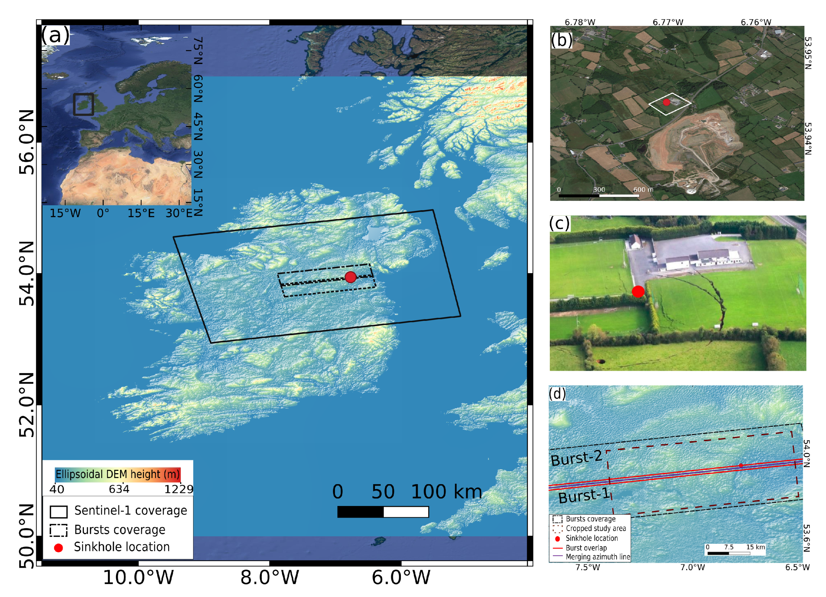
4. SAR Data and Test Site Description

A total of 75 Sentinel-1A SAR images with track number 1 and frame numbers varying between 170 and 175, acquired between 15 April 2015 and 31 December 2018 with a 12-day repeat cycle, were used in this study. All SAR images were obtained in ascending orbital direction, IW mode, and VV polarization channel, see

Table 2. Dataset description.

Data	Date Range	Source	Description
Sentinel-1 SLC SAR	April 2015–December 2018	Alaska Satellite Facility (ASF)	Polarization: VV, Nr. images: 75
			Acquisition mode: IW, Track nr.: 1
Sentinel-1 Orbit data	April 2015–December 2018	Copernicus Sentinels POD Data Hub	Orbit type: Precise

. Figure 4a shows the study area located in North Eastern Ireland, while Figure 4b shows the zoomed-in area. It is in this area that a sinkhole occurred, see Figure 4c. Figure 4a also depicts the Sentinel-1A image boundary at the first acquisition date, as well as the two adjacent bursts in the black dashed line. Figure 4d shows the cropped region from the merged bursts used for this study using a brown dashed line, with the earlier and latter bursts labeled as Burst-1 and Burst-2 respectively.

This sinkhole, shown as the red dot in Figure 4a–c, occurred on 25 September 2018 and its size was reported to be in the order of 100 m [36]. Figure 4c shows an areal picture taken immediately after the sinkhole had occurred. This sinkhole had been attributed to underground activities in a Gypsum mine which can be observed at the bottom of the sinkhole spot Figure 4b [37]. Historically, this is not a sinkhole-prone area. However, the area is situated in a karst region and is rich in gypsum and limestone [38]. For these reasons, the type of sinkhole resembles a combination of a dropout and collapse doline.

5. Results

This section presents the results of the study, in response to the subsections in Section 3.

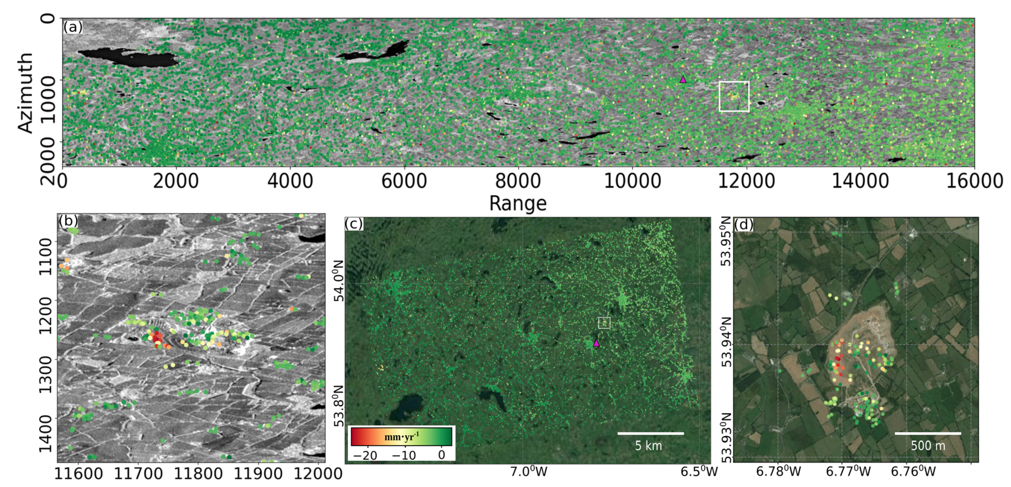
5.1. TSInSAR Results

A total number of 294,519 CCS (i.e., PS) were identified in the cropped study area with size 63.73 km × 43.84 km in east and north direction, respectively, using standard PSI approach with DePSI. Shuttle Radar Topography Mission (SRTM) 1 arc second resolution DEM data [39] was used to remove the reference DEM phase from the interferograms. The CCS locations were obtained in radar coordinate system, see Figure 5a, and in World Geodetic System WGS-84 coordinate reference system (CRS) see Figure 5c. The coordinates in WGS84 CRS were projected onto the local Universal Transverse Mercator (UTM) coordinate system (EPSG code: 2157) and thus used in sinkhole simulation and scanning steps. However, all the results are presented in the WGS84 CRS to ensure consistency. The pink triangle in Figure 5a,c shows the location of the reference point relative to which the deformations are estimated.

During the postprocessing of the PSI results, additional filtering was performed by applying thresholds on ensemble coherence (>0.2), deformation velocity (<5 mm yr${}^{-1}$ and >−25 mm yr${}^{-1}$), and spatio-temporal consistency (STC > 0.008) [40]. The threshold on the ensemble coherence was applied in order to reduce noisy CCS, i.e., CCS with noise in the deformation time series. Moreover, the thresholds on deformation velocities removed CCS with unrealistic deformation velocities, e.g., unusual uplift of points by velocity >5 mm yr${}^{-1}$. This filtering step resulted in a large reduction of noisy CCS, as the total number of CCS reduced to 46,611. A general stable trend was visualized over the cropped study area, see Figure 5a,c. Interestingly, there were a few points in the center of Figure 5b,d with high deformation velocities ($\sim -20$ mm yr${}^{-1}$). These points are located in the mine area that is $\sim 100$ m away from the rim of the sinkhole.

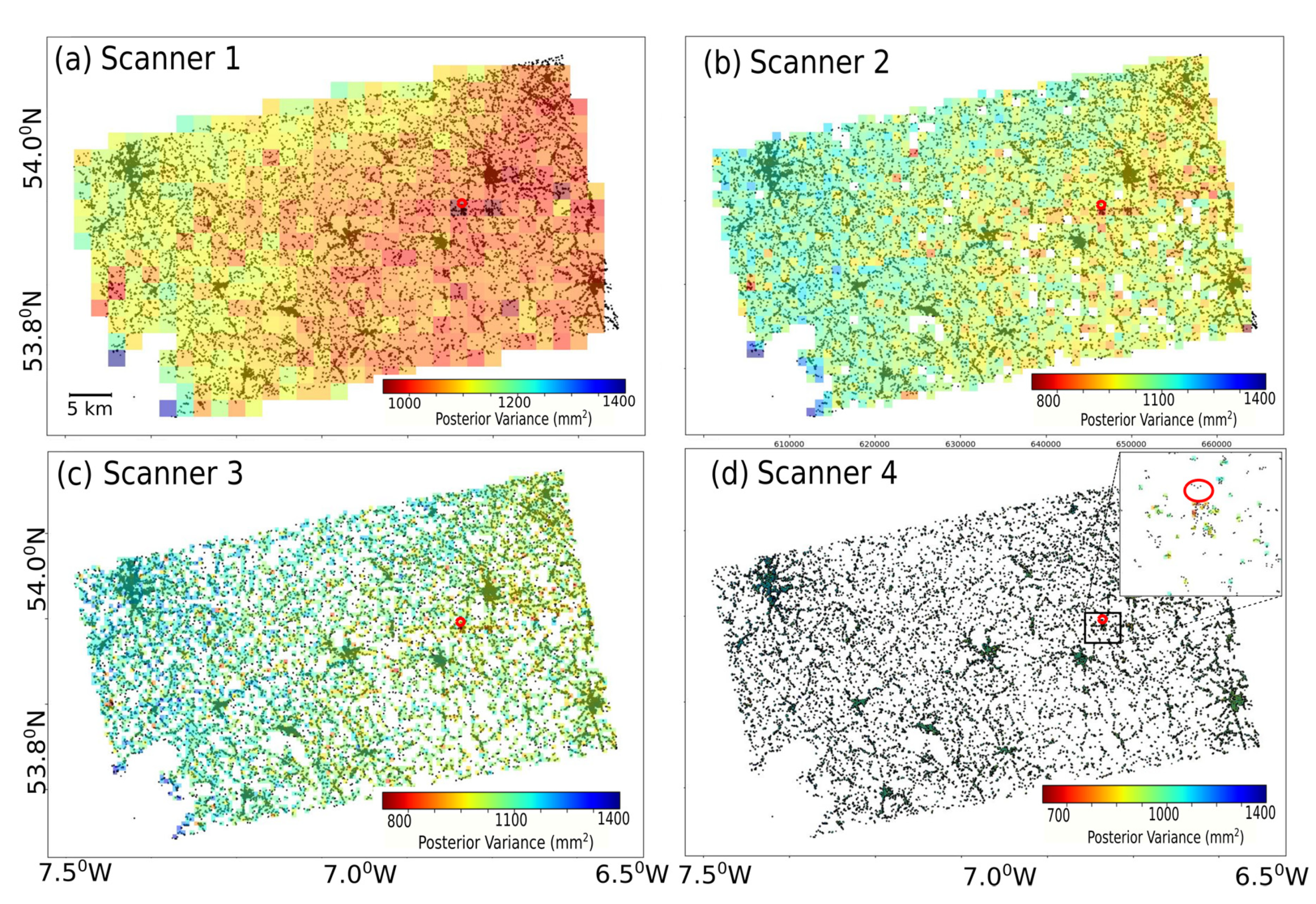
5.2. Sinkhole Scanner Results

We now describe the results from the Sinkhole Scanner step.

Case: Simulation

The two-dimensional horizontal space was divided into grids of $10\times 10$ m, which became the minimum mapping unit for the simulation and for scanning of sinkholes. The common deformation time series of sinkhole centers was defined between $-0.5$ and $-100$ mm varying linearly over the temporal baseline between 0 and $3.65$ years, with a discretization of 10 intervals or epochs. This temporal model was used along with spatial simulation models described in Table 1. The spatial models were defined over the grid defined above. These simulation parameters are summarized in

Table 3. Sinkhole simulation common parameters used for simulating sinkholes.

Parameter	Value
Simulation grid size (m)	10 × 10
Extent of grid ($x,y$) (km)	63.73 ×43.84
Starting depth of sinkhole (mm)	0.5
Maximum depth of center (mm)	100
Temporal baseline (min, max) (year)	(0, 3.65)
Epochs	10
Uncertainty (e) (mm)	10
Velocity of center (mm · yr${}^{-1}$)	25

.

The experiments were designed to simulate and scan sinkholes with sizes ranging from large $\sim 200$ m, to small <∼10 m. Therefore, simulations were conducted with two different sets of values for window size and stride parameters, i.e., a common size of 2000 m and 100 m in both directions. These simulated sinkholes as well as real deformation data were scanned using the Sinkhole Scanner with common window-size and stride values of 2 km, 1 km, 500 m, and 100 m. Window-sizes and stride parameters were chosen to be $\sim 10$ times the size of the sinkhole which is being looked for. This factor was chosen to ensure the intersection of enough CCS to solve the mathematical model. The least number of CCS required to attempt the mathematical model solution was 3, because the number of unknown parameters were 2 in all sinkhole shapes. With this setup, the aim is to find the optimal parameters to model the simulated sinkholes, and sinkhole-shaped patterns in the real data, using the Sinkhole Scanner. The stochastic model was designed as a scaled identity matrix in which ${\sigma }^2=5{\mathrm{mm}}^2$ based on experimental test. We assume that the spatial correlation of CCS which are further away from each other was assumed to be marginal for this study.

Table 4. The parameters for the sinkhole simulation and scanning.

Simulation Space
	Scenario S	Scenario L
Window size (m)	100 × 100	2000 × 2000
Stride (m)	100 × 100	2000 × 2000
${\zeta }_x$, ${\zeta }_y$	(5,5)	(50, 50)
Scanning Space
	Scanner 1	Scanner 2	Scanner 3	Scanner 4
Window size (m)	2000 × 2000	1000 × 1000	500 × 500	100 × 100
Stride (m)	2000 × 2000	1000 × 1000	500 × 500	100 × 100

illustrates the choices for the window sizes and stride parameters in the simulation and scanning space.

Case: Scanning Simulated Data

Figure 6 shows the simulation and scanning results using the Gaussian model. Figure 6a shows the contour plot of the simulated sinkholes which were simulated using Scenario-L, draped over CCS locations shown as black dots. Figure 6b shows the corresponding simulated deformation velocity map over CCS locations. High deformation velocity circular zones can be observed at regular intervals over CCS locations. Finally, Figure 6c shows the application of Scanner 3 (window-size = 500 m) on the simulated data. The map shows goodness of fit of the Gaussian mathematical model for each 500 m × 500 m scanning window. The quality statistic for goodness of fit is the posterior variance. The scattered white patches in the map show regions with insufficient number of CCS to solve the mathematical model. A regular pattern of low posterior variance zones was observed, as expected over low subsidence zones. This can be seen better in the zoomed in image in Figure 6d, corresponding to the black box in Figure 6c. However, low posterior variance zones were observed in windows where the CCS density was sufficient to recreate the sinkhole shape. This regular pattern shows that this scanning method can highlight low subsidence zones with respect to relatively stable regions. We show the results from Scanner 3, which provided the best results of all the four scanners. Note that the best performing window size in this case was ∼10 times the $\zeta$ parameter chosen for the simulated sinkholes. However, limited success was observed while scanning for sinkhole simulation Scenario-S using any of the scanners. This may have been due to either too many sinkholes in case of a large window size (e.g., Scanner 1) or too few CCS intersected in case of a small window size (Scanner 4). In addition, we observed that the model was able to correctly estimate the v parameter with an error of under 5%, whereas the parameter $\zeta$ was overestimated which may be due to the finite value of the parameter $\delta$.

Case: Scanning Real Data

Figure 7 shows the result of scanning real deformation data using all four Sinkhole Scanners, i.e., Scanner 1–4, using the Gaussian shape in Figure 7a–d, respectively. In the case of Scanner 1 (Figure 7a), a trend of better fitting grids was observed when moving from west to east. This is also slightly evident in the case of smaller window sizes as well, see Figure 7b,c. As the window size decreases, this trend is observed to converge near the actual sinkhole location.

We also observed that the range for posterior variance values widens as we decrease the window size. This is because the lower bound of the values decreases, but the upper bound remains almost the same. The absolute values of posterior variance are high. This is likely due to the finite value of the $\delta$ parameter used in the functional model to elevate the deformation values above zero. This causes a Gaussian to be modeled considerably above the zero deformation value, and causes a bias between the modeled and original observations. However, as the $\delta$ is constant and chosen to the smallest deformation value in the observation space, its effect in space is consistent. This, however, leads to a higher dynamic range in the posterior variance values and therefore a higher contrast in the goodness of fit map, which helps in identifying vulnerable areas much better. This offset can be reduced by employing more flexible models, or by using Taylor expansions. Furthermore, we observed that reducing the window size of the scanner resulted in a finer resolution sinkhole scanning map, however at the cost of a reduced scanned area due to the nonuniform CCS distribution.

Table 5. Scanned grids and area by Sinkhole Scanner.

Scanner	Total Grids	Nr. of Scanned Grids	Scanned Area (km${}^2$)
Scanner 1	651	499	1996
Scanner 2	2709	1142	1142
Scanner 3	10,922	2819	704.75
Scanner 4	274,320	1964	19.64

shows the variation of scanned area with reducing window size.

Contrasting results were observed for the Cylindrical and Conical sinkholes where the trend of fitting was opposite to the Gaussian model. High posterior variance values were observed for sinkhole zones as compared to stable areas. This suggests that the Gaussian model is best suited for modeling sinkholes in this area. The values of posterior variance were much lower than in the Gaussian case, most likely due to the absence of the offset parameter $\delta$ in the observation vector. However, the contrast between fitting zones was less pronounced than in the Gaussian case.

The estimated velocities for the windows also showed high deformation rate near the sinkhole area, see Figure 8b. On comparison with the window-wise (Scanner 4) spatially averaged InSAR derived deformation velocities of CCS, see Figure 8a, we notice that the model overestimates the deformation velocities Figure 8c. This is likely due to spatial averaging of the deformation velocities.

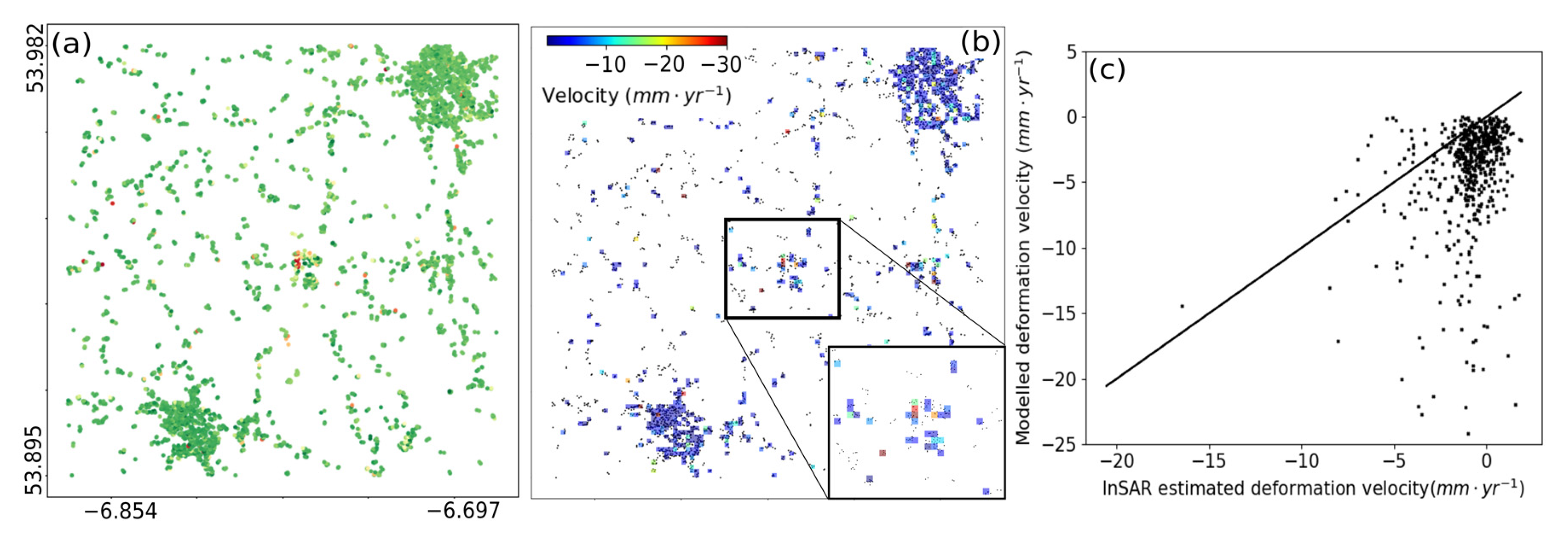
5.3. Hypothesis Testing Results

Figure 9 shows the deformation velocity map and deformation time series of CCS located near the sinkhole site. The results show a large deformation velocity near the sinkhole site, as shown in Figure 9a. The points are annotated and their corresponding deformation time series over 75 epochs is shown in Figure 9b. We observed that a few epochs before the sinkhole event, there was a sudden change in the behaviour of the deformation time series of CCS lying over the mining region, close to the sinkhole site. The change is in the form of sudden deformation velocity change approximately 10 epochs before the sinkhole.

In order to validate any such anomalies, we use multiple hypothesis testing (MHT), to automatically detect any such behaviour. The level of significance was initially defined as $\alpha =1/\left(2m\right)=1/(2\times 74)\approx 0.68\%$ and the power of the test $\gamma$ was chosen to be $50\%$. The horizontal axis of Figure 10 shows the temporal baseline, and each colored time series shows the test ratio statistic for the Heaviside and Breakpoint model in Figure 10a,b, respectively, for each CCS. For instance, we can notice a sudden drop in the deformation for PS2 (time series in orange) at the 24th epoch, (temporal baseline = 1.085 yr), in Figure 9b. Corresponding to the 24th epoch, we can observe spikes in the corresponding test ratio statistic time series for both Heaviside and Breakpoint anomaly (also shown in orange). This way, MHT is able to detect the best deformation model from a set of deformation functions.

Figure 10 shows that the highest value of test ratio statistic was for PS1, which indicates that these anomalies are more apparent in the deformation time series of PS1 as compared to other CCS. Furthermore, Figure 10a shows that there are high indications of Heaviside jumps for CCS above PS8 and PS9, at the epoch corresponding to the sinkhole event. Moreover, Breakpoint test ratio increases for PS6 just before the sinkhole occurrence. PS6, PS8, and PS9 are situated directly above the sinkhole site.

The results from the Sinkhole Scanner were compared with the results from the Hypothesis testing method. Both the methods give relative information about only temporal anomalies with MHT, and both spatial and temporal anomalies with Sinkhole Scanner. The Sinkhole Scanner gives a map of sinkhole similarity for a large area because of its grid-wise operation, and is not limited to give information only over the CCS point locations. The MHT method gives results only in time, which can be projected onto the CCS point location in space, as done in [41], but cannot extend to give information of a spatial trend in the result. However, MHT is not limited to the CCS number threshold required to deliver a result as in the case of Sinkhole Scanner.

6. Discussion

One of the most interesting observations in this work was the identification of large deformations near the sinkhole site in Ireland. This was observed in the deformation velocity map in Ireland. These observations were valuable and fortunate because of the orientation of mining terraces to the radar line of sight which acted as double bounce scatterers. This would otherwise not have been possible because of the large number of vegetation scatterers. The advantage of using CCS was a higher accuracy in geolocation and deformation estimates, although at the expense of lesser number of measurement locations. The subsidence over the sinkhole area was attributed to a mine collapse [42]. The collapse of the mine was approximately 50 m away from the periphery of the sinkhole. This information, along with the InSAR subsidence data, were sufficiently convincing that the deformation was related to the unstable ground over the mining area, and that its collapse led to the sinkhole. Validation using in situ reference data could not be performed because of their unavailability near the sinkhole spot. As soon as reference data, e.g., from GPS or extensometers are available, the InSAR signals can be validated [43] and thus used to verify actual anomalous activities in space and time. Further ancillary information, e.g., groundwater table can help in identifying signals due to sinkholes from other geo-processes.

The major contribution of this study was the Sinkhole Scanner which was defined to model the LOS deformation time series over CCS. It was assumed that that the LOS direction was sensitive to the sinkhole-related deformation in the vertical direction. The scanner was defined using a 4-dimensional moving window-based method in space and time, where a 3-dimensional sinkhole model, like an inverted Gaussian function evolving in time, is fitted to the CCS deformation time series overlapped by the moving window using least-squares estimation. The Gaussian function was simplified such that there were only two unknown parameters: the extent of the Gaussian function $\zeta$ of the circular shaped Gaussian, and the linear deformation velocity v of the center of the Gaussian function. The stochastic model used for estimating the unknown vector was an identity matrix scaled to a common variance.

The results from the Sinkhole Scanner show its effectiveness in detecting sinkhole-like evolving spatio-temporal deformation patterns. The four Sinkhole Scanners, designed to detect sinkholes at different resolutions were all able to detect Gaussian shaped sinkhole subsidence patterns. This was validated using the sinkhole simulation experiment and was especially evident in the area around the real sinkhole location. However, it is not easily observed in the deformation velocity map. Therefore, the Sinkhole Scanner is well applicable when using spatio-temporal deformation data in modeling such subsidence patterns. Furthermore, Scanners 1–3 highlight the grid containing the sinkhole area to be the most sinkhole-like deforming region. This establishes that the Sinkhole Scanner is useful in detecting sinkhole-like features. The Gaussian shape model, in contrast to Cylinder and Conical shape model, showed the best results in terms of fitting better to sinkhole zones as compared to stable areas. This fits well with the Karst geology of the terrain where Gaussian shaped sinkholes are more likely to occur [4].

From Scanners 1–4, the lower-bound of the posterior variance range reduces which may indicate improved Gaussian shaped patterns at a fine spatial scale. Unfortunately, the coarse CCS density does not allow us to investigate this further, but this can be done with higher spatial resolution datasets, e.g., Spanish PAZ SAR data [44].

The mathematical model for the Gaussian shape was defined to identify sinkhole-shaped patterns with the center of the sinkhole lying at the center of the search window. It may happen that the sinkhole is located at the peripheries of the search window. In that case, the stride parameter can be reduced to ensure that the center of the search window aligns with the potential sinkhole center. It may also happen that there may be more than one sinkholes in the same search window. In that case, the window size of the scanner can be further reduced. The scanning results were dependent upon the CCS point density. When the scanning window size decreased, the number of CCS points overlapped by the scanning window also decreased and thus reducing the scanned area. For instance, the scanned area reduced by almost 100 times by reducing the window size from 2 km to 100 m. However, the fine-resolution map made with Scanner 4 helped in highlighting the location of sinkhole and also identified the best fitting locations with lower posterior variance values than the other three scanners. Furthermore, the spatial resolution of the radar is important when choosing a window size. A finer resolution image would give a higher density of CCS, which can be worked upon by even smaller Sinkhole Scanner window sizes.

The results also showed that the MHT is able to identify Heaviside anomalies in two CCS a few epochs before the sinkhole occurrence. MHT method can be used as another tool to identify temporal anomalies which can indicate vulnerable areas. The Sinkhole Scanner, in conjunction with MHT can be useful in detecting sinkhole related subsidence. The Sinkhole Scanner can thus be used for performing a global search over a sinkhole affected area, followed by Hypothesis testing to further investigate sinkhole-related anomalies.

In this research, we extended the research in [20]. We used more robust models, better model fitting methods, worked on a coarser resolution data and worked on a larger study area in a non-sinkhole prone region. However, several limitations still exist to the work. The major one is that we have used a general stochastic model for the Sinkhole Scanner. A more detailed stochastic model can be used to take the uncertainty in the deformation estimation into account [45]. Furthermore, a simplified Gaussian function was used to detect sinkholes, whereas the deformation behaviour can be more complex.

7. Conclusions

This study presents the Sinkhole Scanner, which includes methods to identify spatio-temporal changes in CCS behavior. The method is robust in the sense that different sinkhole shaped models can be used in place of the Gaussian function, e.g., a cylinder, a cone, or even a more flexible Gaussian function. Four different variants of the Sinkhole Scanners with different window sizes were used to identify sinkholes in simulated and real deformation time series. The scanner showed ∼30% lower posterior variance values over the sinkhole areas for both simulated and real datasets. Moreover, it showed a high contrast in the posterior variance values for windows near the sinkhole area. This was not visible from the deformation velocity map. Therefore, the Sinkhole Scanner provides additional information about sinkhole shaped spatio-temporal patterns, as compared to the deformation velocity map. Furthermore, Gaussian shaped sinkhole performed best in highlighting correct contrast between sinkholes and stable zones.

A trade-off was identified between the model’s ability to detect smaller sinkholes and the number of windows with no solution to the least squares model. In this study area, there was 100 times reduction in the area returning successful model fitting from a larger Scanner 1 to a finer Scanner 4. The deformation velocity map over Ireland showed high deformation velocity near the mining area. This deformation trend suggested precursory deformation patterns in both space and time around the mining area. Sinkhole Scanners 1–3 were able to identify Gaussian-shaped patterns over the real sinkhole area. In the case study, Scanner 3 performs best role of providing high coverage area, and also highlighting the sinkhole location. In addition to real deformation data, deformation data were extracted from a simulated sinkhole field. The simulated data gave sufficient evidence of providing contrast between sinkhole and non-sinkhole areas. In the simulation case, the window size of 500 × 500 m also provided the best results. The study suggests that multiple window sizes should be tested to get an idea of the spatial trend of posterior variance in the area. Smaller window size can be further tested in areas with relatively lower values of posterior variance. This would also considerably reduce the scanning time.

Future studies may consider learning-based algorithms [46] to identify anomaly types, while convolution filters [47] with successive lowering of the window size can be explored to encode information at various scales and then decode it to identify sinkhole shaped deformation patterns. Furthermore, a more complex stochastic model in InSAR processing can be used, see, e.g., in [45]. The addition of DS-InSAR would also be useful in increasing the InSAR measurement point density. Distributed Scatterers [48], and Temporary Coherent Scatterers [49] would help in increasing the number of measurement locations. Their precise role should be explored in future studies. A priori contextual information about the size and shape of the brewing sinkholes can be used for choosing the window size of the scanner and sinkhole shape, respectively. Finally, in the MHT step, more and physically realistic number of the breaks or jumps could be added to the models.

References

1. Al-Halbouni, D.; P Holohan, E.; Taheri, A.; Schöpfer, M.P.; Emam, S.; Dahm, T. Geomechanical modelling of sinkhole development using distinct elements: Model verification for a single void space and application to the Dead Sea area. Solid Earth 2018, 9, 1341–1373. [Google Scholar] [CrossRef] [Green Version]
2. Theron, A.; Engelbrecht, J. The Role of Earth Observation, with a Focus on SAR Interferometry, for Sinkhole Hazard Assessment. Remote Sens. 2018, 10, 1506. [Google Scholar] [CrossRef] [Green Version]
3. Jain, S. Fundamentals of Physical Geology; Springer: New Delhi, India, 2014; pp. 227–238. [Google Scholar] [CrossRef]
4. Williams, P. Encyclopedia of Caves and Karst Science; Chapter Dolines; Fitzroy Dearborn: New York, NY, USA, 2004; pp. 304–310. [Google Scholar] [CrossRef]
5. Desir, G.; Merino, J.; Carbonel, D.; Benito Calvo, A.; Guerrero, J.; Fabregat, I. Rapid subsidence in damaging sinkholes: Measurement by high-precision leveling and the role of salt dissolution. Geomorphology 2018, 303, 393–409. [Google Scholar] [CrossRef]
6. Maheshwari, M.; Yang, Y.; Upadrashta, D.; Huang, E.S.; Goh, K.H. Fiber Bragg Grating (FBG) based magnetic extensometer for ground settlement monitoring. Sens. Actuators A Phys. 2019, 296, 132–144. [Google Scholar] [CrossRef]
7. Wust-Bloch, G.H.; Joswig, M. Pre-collapse identification of sinkholes in unconsolidated media at Dead Sea area by ‘nanoseismic monitoring’ (graphical jackknife location of weak sources by few, low-SNR records). Geophys. J. Int. 2006, 167, 1220–1232. [Google Scholar] [CrossRef] [Green Version]
8. Suh, J.; Choi, Y. Mapping hazardous mining-induced sinkhole subsidence using unmanned aerial vehicle (drone) photogrammetry. Environ. Earth Sci. 2017, 76. [Google Scholar] [CrossRef]
9. Lee, E.J.; Shin, S.Y.; Ko, B.C.; Chang, C. Early sinkhole detection using a drone-based thermal camera and image processing. Infrared Phys. Technol. 2016, 78, 223–232. [Google Scholar] [CrossRef]
10. Love, A. In Memory of Carl A. Wiley. IEEE Antennas Propag. Soc. Newsl. 1985, 27, 17–18. [Google Scholar] [CrossRef]
11. Torres, R.; Snoeij, P.; Geudtner, D.; Bibby, D.; Davidson, M.; Attema, E.; Potin, P.; Rommen, B.Ö.; Floury, N.; Brown, M.; et al. GMES Sentinel-1 mission. Remote Sens. Environ. 2012, 120, 9–24. [Google Scholar] [CrossRef]
12. Yaseen, M.; Hamm, N.; Woldai, T.; Tolpekin, V.; Stein, A. Local interpolation of coseismic displacements measured by InSAR. Int. J. Appl. Earth Obs. Geoinf. 2013, 23, 1–17. [Google Scholar] [CrossRef]
13. Amelung, F.; Galloway, D.L.; Bell, J.W.; Zebker, H.A.; Laczniak, R.J. Sensing the ups and downs of Las Vegas: InSAR reveals structural control of land subsidence and aquifer-system deformation. Geology 1999, 27, 483–486. [Google Scholar] [CrossRef]
14. Markušić, S.; Stanko, D.; Penava, D.; Ivančić, I.; Bjelotomić Oršulić, O.; Korbar, T.; Sarhosis, V. Destructive M6.2 Petrinja Earthquake (Croatia) in 2020—Preliminary Multidisciplinary Research. Remote Sens. 2021, 13, 1095. [Google Scholar] [CrossRef]
15. Ferretti, A.; Prati, C.; Rocca, F. Permanent Scatters in SAR Interferometry. IEEE Trans. Geosci. Remote Sens. 2001, 39, 8–20. [Google Scholar] [CrossRef]
16. Hooper, A.; Zebker, H.; Segall, P.; Kampes, B. A new method for measuring deformation on volcanoes and other natural terrains using InSAR persistent scatterers. Geophys. Res. Lett. 2004, 31, 1–5. [Google Scholar] [CrossRef]
17. Lanari, R.; Mora, O.; Manunta, M.; Mallorquí, J.J.; Berardino, P.; Sansosti, E. A small-baseline approach for investigating deformations on full-resolution differential SAR interferograms. IEEE Trans. Geosci. Remote Sens. 2004, 42, 1377–1386. [Google Scholar] [CrossRef]
18. Chang, L.; Hanssen, R.F. Detection of cavity migration and sinkhole risk using radar interferometric time series. Remote Sens. Environ. 2014, 147, 56–64. [Google Scholar] [CrossRef]
19. Nof, R.N.; Abelson, M.; Raz, E.; Magen, Y.; Atzori, S.; Salvi, S.; Baer, G. SAR interferometry for sinkhole early warning and susceptibility assessment along the Dead Sea, Israel. Remote Sens. 2019, 11, 89. [Google Scholar] [CrossRef] [Green Version]
20. Vaccari, A.; Stuecheli, M.; Bruckno, B.; Hoppe, E.; Acton, S.T. Detection of geophysical features in InSAR point cloud data sets using spatiotemporal models. Int. J. Remote Sens. 2013, 34, 8215–8234. [Google Scholar] [CrossRef]
21. Baer, G.; Magen, Y.; Nof, R.N.; Raz, E.; Lyakhovsky, V.; Shalev, E. InSAR Measurements and Viscoelastic Modeling of Sinkhole Precursory Subsidence: Implications for Sinkhole Formation, Early Warning, and Sediment Properties. J. Geophys. Res. Earth Surf. 2018, 123, 678–693. [Google Scholar] [CrossRef]
22. Kim, J.W.; Lu, Z.; Degrandpre, K.; Kim, J.W.; Lu, Z.; Degrandpre, K. Ongoing Deformation of Sinkholes in Wink, Texas, Observed by Time-Series Sentinel-1A SAR Interferometry (Preliminary Results). Remote Sens. 2016, 8, 313. [Google Scholar] [CrossRef] [Green Version]
23. Malinowska, A.A.; Witkowski, W.T.; Hejmanowski, R.; Chang, L.; van Leijen, F.J.; Hanssen, R.F. Sinkhole occurrence monitoring over shallow abandoned coal mines with satellite-based persistent scatterer interferometry. Eng. Geol. 2019, 262, 105336. [Google Scholar] [CrossRef]
24. Martinotti, M.E.; Pisano, L.; Marchesini, I.; Rossi, M.; Peruccacci, S.; Brunetti, M.T.; Melillo, M.; Amoruso, G.; Loiacono, P.; Vennari, C.; et al. Landslides, floods and sinkholes in a karst environment: The 1–6 September 2014 Gargano event, southern Italy. Nat. Hazards Earth Syst. Sci. 2017, 17, 467–480. [Google Scholar] [CrossRef] [Green Version]
25. Chang, L.; Hanssen, R.F. A Probabilistic Approach for InSAR Time-Series Postprocessing. IEEE Trans. Geosci. Remote Sens. 2016, 54, 421–430. [Google Scholar] [CrossRef] [Green Version]
26. Jones, C.E.; Blom, R.G. Bayou Corne, Louisiana, sinkhole: Precursory deformation measured by radar interferometry. Geology 2014, 42, 111–114. [Google Scholar] [CrossRef]
27. Hermosilla, R.G. The Guatemala City sinkhole collapses. Carbonates Evaporites 2012, 27, 103–107. [Google Scholar] [CrossRef]
28. Yague-Martinez, N.; Prats-Iraola, P.; Gonzalez, F.R.; Brcic, R.; Shau, R.; Geudtner, D.; Eineder, M.; Bamler, R. Interferometric Processing of Sentinel-1 TOPS data. IEEE Trans. Geosci. Remote Sens. 2016, 54, 2220–2234. [Google Scholar] [CrossRef] [Green Version]
29. Hanssen, R.F. Radar Interferometry: Data Interpretation and Error Analysis; Springer: Dordrecht, The Netherlands, 2001. [Google Scholar] [CrossRef] [Green Version]
30. Kampes, B.M. Radar Interferometry: Persistent Scatterer Technique (Remote Sensing and Digital Image Processing); Springer: Dordrecht, The Netherlands, 2006; pp. 1–383. [Google Scholar]
31. van Leijen, F. Persistent Scatterer Interferometry Based on Geodetic Estimation Theory. Ph.D. Thesis, Delft University of Technology, Delft, The Netherlands, 2014. [Google Scholar]
32. Kampes, B.M.; Hanssen, R.F. Delft Object-Oriented Radar Interferometric Software: Users Manual and Technical Documentation; Technical Report; Delft University of Technology: Delft, The Netherlands, 2008. [Google Scholar]
33. Miranda, N.; Small, D.; Schubert, A.; Meadows, P.; Hajduch, G. Guide to Sentinel-1 Geocoding; Technical Report; University of Zurich: Zurich, Switzerland, 2019. [Google Scholar]
34. Piantanida, R. Sentinel-1 Level-1 Detailed Algorithm Definition; Technical Report; ESA: Paris, France, 2019. [Google Scholar]
35. Teunissen, P.J.G.; Simons, D.G.; Tiberius, C.C.J.M. Probability and Observation Theory; Delft University of Technology: Delft, The Netherlands, 2005. [Google Scholar]
36. Sinkhole-Hit GAA Club in County Monaghan Plans New Pitches. Available online: https://www.bbc.com/news/world-europe-46748729 (accessed on 3 January 2019).
37. Bowers, S. Large Hole Reappears on Lands Near Mining Network in Co Monaghan. Available online: https://bit.ly/3p4ZPoh (accessed on 20 January 2020).
38. Geological Survey-Geohazards. Geological Survey of Ireland. Available online: https://www.gsi.ie/en-ie/data-and-maps/Pages/Geohazards.aspx (accessed on 29 December 2020).
39. van Zyl, J.J. The Shuttle Radar Topography Mission (SRTM): A breakthrough in remote sensing of topography. Acta Astronaut. 2001, 48, 559–565. [Google Scholar] [CrossRef]
40. Cuenca, M.C. Improving Radar Interferometry for Monitoring Fault-Related Surface Deformation. Ph.D. Thesis, Delft University of Technology, Delft, The Netherlands, 2013. [Google Scholar]
41. Van De Kerkhof, B.; Pankratius, V.; Chang, L.; Van Swol, R.; Hanssen, R.F. Individual Scatterer Model Learning for Satellite Interferometry. IEEE Trans. Geosci. Remote Sens. 2020, 58, 1273–1280. [Google Scholar] [CrossRef]
42. Geoengineer. Huge Sinkhole Caused by Mine Collapse in Ireland. Available online: https://www.geoengineer.org/news/huge-sinkhole-caused-by-mine-collapse-in-ireland (accessed on 12 October 2018).
43. Qu, F.; Lu, Z.; Zhang, Q.; Bawden, G.W.; Kim, J.W.; Zhao, C.; Qu, W. Mapping ground deformation over Houston–Galveston, Texas using multi-temporal InSAR. Remote Sens. Environ. 2015, 169, 290–306. [Google Scholar] [CrossRef]
44. Chang, L.; Stein, A. Exploring PAZ co-polarimetric SAR data for surface movement mapping and scattering characterization. Int. J. Appl. Earth Obs. Geoinf. 2021, 96, 102280. [Google Scholar] [CrossRef]
45. Ketelaar, G.; Bähr, H.; Liu, S.; Piening, H.; Van Der Veen, W.; Hanssen, R.; Van Leijen, F.; Van Der Marel, H.; Samiei-Esfahany, S. Integrated monitoring of subsidence due to hydrocarbon production: Consolidating the foundation. Proc. Int. Assoc. Hydrol. Sci. 2020, 382, 117–123. [Google Scholar] [CrossRef] [Green Version]
46. Gers, F.A.; Schmidhuber, J.; Cummins, F. Learning to Forget: Continual Prediction with LSTM. Neural Comput. 1999, 12, 2451–2471. [Google Scholar] [CrossRef] [PubMed]
47. Zhu, X.X.; Montazeri, S.; Ali, M.; Hua, Y.; Wang, Y.; Mou, L.; Shi, Y.; Xu, F.; Bamler, R. Deep Learning Meets SAR. IEEE Geosci. Remote Sens. Mag. 2020, 1–23. [Google Scholar] [CrossRef]
48. Samiei-Esfahany, S.; Martins, J.E.; Van Leijen, F.; Hanssen, R.F. Phase Estimation for Distributed Scatterers in InSAR Stacks Using Integer Least Squares Estimation. IEEE Trans. Geosci. Remote Sens. 2016, 54, 5671–5687. [Google Scholar] [CrossRef] [Green Version]
49. Hu, F.; Wu, J.; Chang, L.; Hanssen, R.F. Incorporating Temporary Coherent Scatterers in Multi-Temporal InSAR Using Adaptive Temporal Subsets. IEEE Trans. Geosci. Remote Sens. 2019, 57, 7658–7670. [Google Scholar] [CrossRef] [Green Version]
50. ESA. Copernicus Open Access Hub; ESA: Paris, France, 2021. [Google Scholar]
Figure 1. (a) A sinkhole at an early development stage [1]. The surface S subsides due to the presence of a dissolution zone C underneath the surface. Side views of (b) Gaussian, (c) Cylindrical, and (d) Conical simulated sinkholes. (e) Top view of the sinkhole spot with 30 randomly distributed InSAR CCS, and rendered structure of sinkholes with these 30 CCS for (f) Gaussian, (g) Cylindrical, and (h) Conical shape.
Remotesensing 13 02906 g001
Figure 2. Methodological flow diagram.
Remotesensing 13 02906 g002
Figure 3. Conical shaped sinkhole geometry. The sinkhole has the center at O and subsides by time t to point B , a surface measurement point P i located at ( x i , y i ) subsides to point D at time t .
Remotesensing 13 02906 g003
Figure 4. (a) Sentinel-1A spatial coverage and test site location superimposed on an ellipsoidal height DEM map, (b) zoomed-in optical image, and (c) areal image taken after the sinkhole occurred, covering the area shown by the white quadrilateral in subfigure (b), (d) overlapped burst area (red rectangle), azimuth merge line, and cropped area used for the study.
Remotesensing 13 02906 g004
Figure 5. CCS distribution and deformation velocity map over (a) the cropped study area and (b) the subset corresponding to the white box in subfigure (a), in radar coordinates. Deformation trend in WGS84 coordinate system (c), and zoomed in over the sinkhole area (d) corresponding to the white box in subfigure (c). Note that the cluster of red CCS over the mining site is near the sinkhole site. The pink triangle shows the reference point location.
Remotesensing 13 02906 g005
Figure 6. Sinkhole simulation and scanning with Gaussian shape. (a) CCS distribution and contour plot for simulated sinkhole depth at the last simulation epoch, simulation Scenario L, (b) the equivalent simulated sinkhole deformation velocity map, (c) Posterior variance after scanning using Scanner 1 for Gaussian sinkholes over the simulated data, (d) zoomed in image corresponding to the black box in (c).
Remotesensing 13 02906 g006
Figure 7. Sinkhole scanning using Gaussian shape for real sinkholes using 4 window sizes: (a) 2 km, (b) 1 km, (c) 500 m, and (d) 100 m, with a zoomed-in image as inset on the top-right of (d). The red ellipse represents the sinkhole rim.
Remotesensing 13 02906 g007
Figure 8. Original InSAR estimated velocities (a) and modelled velocities (b) using Sinkhole scanning with Gaussian shape for real sinkholes for window size 100 m, and a scatter-plot plotted between the two (c).
Remotesensing 13 02906 g008
Figure 9. Anomalous deformation behaviour near the sinkhole site. Deformation velocity map (a) and associated deformation time series (b). Significant deformation velocity and deep deformation values can be observed for areas near the sinkhole site.
Remotesensing 13 02906 g009
Figure 10. Test ratio statistic for Heaviside (a) and Breakpoint (b) anomaly models for deformation time series of PS points in Figure 9.
Remotesensing 13 02906 g010