3D Pedestrian Detection in Farmland by Monocular RGB Image and Far-Infrared Sensing

Abstract

The automated driving of agricultural machinery is of great significance for the agricultural production efficiency, yet is still challenging due to the significantly varied environmental conditions through day and night. To address operation safety for pedestrians in farmland, this paper proposes a 3D person sensing approach based on monocular RGB and Far-Infrared (FIR) images. Since public available datasets for agricultural 3D pedestrian detection are scarce, a new dataset is proposed, named as “FieldSafePedestrian”, which includes field images in both day and night. The implemented data augmentations of night images and semi-automatic labeling approach are also elaborated to facilitate the 3D annotation of pedestrians. To fuse heterogeneous images of sensors with non-parallel optical axis, the Dual-Input Depth-Guided Dynamic-Depthwise-Dilated Fusion network (D5F) is proposed, which assists the pixel alignment between FIR and RGB images with estimated depth information and deploys a dynamic filtering to guide the heterogeneous information fusion. Experiments on field images in both daytime and nighttime demonstrate that compared with the state-of-the-arts, the dynamic aligned image fusion achieves an accuracy gain of 3.9% and 4.5% in terms of center distance and BEV-IOU, respectively, without affecting the run-time efficiency.

1. Introduction

In recent years, the widespread application of artificial intelligence in traditional agriculture has drawn increased attention in researches. As one of the representatives, the intelligent farm is conducive to improving the safety and efficiency in agricultural operations. Especially in the process of human-machine cooperation, machines attempt to install sensors for environment perception to avoid accidents with working staff. With progress in computer vision, visual sensors are prioritized for installation on agricultural machinery to perceive surrounding objects like pedestrians.

Existing research such as [1,2] presented approaches for classifying pedestrians using LiDAR point clouds and localizing them with high accuracy. However, their used sensors are relatively expensive which will hinder their commercial application. RGB cameras, with a relative low cost, can also provide rich environmental semantic information. Moreover, monocular camera images have been leveraged by deep learning approaches to detect both 2D and 3D objects. For example, [3,4] proposed perception systems to extract the semantic information from a front-view RGB image in the agricultural field and to warn the driver before a possible pedestrian collision. However, normal cameras can be easily affected by illumination changes or occlusions, which make them less appropriate in dealing with different environmental surroundings through day and night. On the contrary, FIR cameras have a strong response to the thermal radiator and therefore can be implemented as a night vision sensor for pedestrian detection. However, the off-the-shelf resolutions of FIR cameras are strongly limited, and thus the captured object information is not meticulous enough. Moreover, to the best of our knowledge, there are neither public datasets available that address the detection of 3D pedestrians in varied agricultural environments, which has further slowed down the related research.

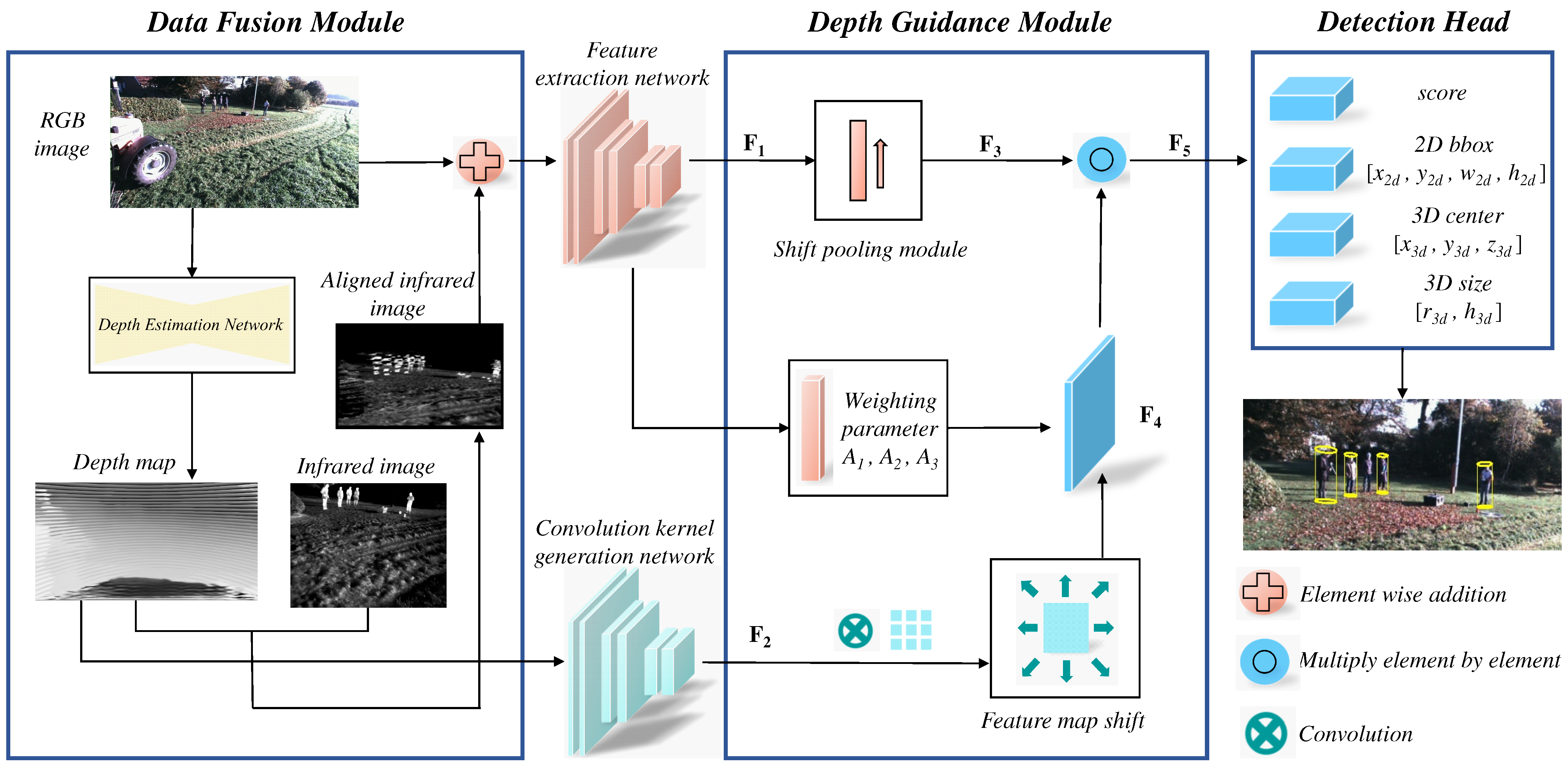
Considering the above issues, this paper strives to build an RGB and FIR image-based approach to detect 3D pedestrians in a low-light agricultural environment. As shown in Figure 1, this paper mainly includes two parts: Dataset generation and 3D pedestrian detection. On the one hand, based on the prior work [5], a new pedestrian detection dataset “FieldSafePedestrian” is proposed with carefully annotated 3D labels and extra augmented nighttime images. The whole labeled dataset is generated by mixing manual and automatic annotation, and utilizing Cycle-GAN [6] and variant illumination channel to expand the nighttime data. On the other hand, the Dual-Input Depth-guided Dynamic-Depthwise-Dilated Fusion network (D5F) is proposed for 3D pedestrian detection in farmland. The architecture deploys estimated depth information to guide the alignment between color and FIR images, and further optimizes their fusion by dynamic filtering and dilation convolutions.

The entire paper is organized as follows. In Section 2, related works are reviewed in aspects of depth estimation, object detection, and the proposed pervasive dateset. Then Section 3 presents the detailed procedure of dataset generation. The proposed pedestrian detection method is described in Section 4. To verify the effectiveness of the proposed method, experiments are presented in Section 5. The paper concludes in Section 6.

2. Related Works

Although a large number of enterprises and universities have carried out research on the unmanned operation of agricultural machinery, there are few studies on 3D pedestrian detection [7] in farmland based on heterogeneous cameras, and related datasets are also scarce. Thus, in this section, we mainly summarize research from aspects of depth estimation, 3D object detection, and datasets related to agriculture and 3D object detection.

2.1. Depth Estimation Based on Monocular and FIR Images

The depth estimation of monocular images is currently based on deep neural networks with the learned parameters to estimate the depth value of each pixel in a camera coordinate system. These researches can mostly be summarized in two aspects, supervised learning and unsupervised learning, according to the availability of groundtruth. Supervised learning-based approaches request the real depth value of each pixel as groundtruth and then estimate depth by regression losses. The prior work for depth estimation based on monocular images was proposed by Eigen et al. [8] and it integrated surface normal estimation and semantic segmentation in a coarse-to-fine manner. Liu et al. [9] and Li et al. [10] combined deep learning and conditional random fields through an energy function to assist depth estimation in both pixel and super-pixel levels. Iro et al. [11] designed a specialized fully convolutional network to establish a fuzzy mapping relationship between the color image and its depth. Unlike previous works, the DORN [12] regarded the depth regression as a classification problem, which makes the network learning much more easier. The work of BTS [13] was proposed to link feature maps from different decoding stages, and geometric plane constraints were added during the network training process. Hereby, the supervised learning strongly relies on depth labels, which are achieved by expensive LiDAR measurement or by stereo vision estimation. However, the LiDAR measurement is sparse and the accuracy of stereo estimation decreases at a far distance. Thus, there are still difficulties in obtaining accurate and dense depth values in traffic scenarios, which increases the difficulty of implementation.

On the other hand, unsupervised learning-based approaches attempt to estimate the depth according to the movement of each pixel in consecutive frames along with the motion state of camera. Zhou et al. [14] designed networks to respectively predict the depth of each pixel and the camera pose. The network was trained by comparing the reconstructed adjacent frame with the real frame, thus no groundtruth for depth value is required. The GeoNet [15] integrated an optical flow estimation module into the previous work, forming a multi-task learning approach for the joint estimation of both depth and camera pose. The MonodepthV2 [16] improved the depth precision with innovative theories including the minimum luminosity reprojection error, the full-resolution multi-scale sampling, and the automatic mask loss function, and achieved state-of-the-art performance. However, depth values estimated by above approaches cannot directly yield object detection results. They are mostly used as auxiliary information to improve the accuracy of 3D pedestrian detection.

2.2. 3D Object Detection Based on Monocular and FIR Images

3D object detection can obtain the 3D pose of an object and thus supplement the depth and spatial size of 2D detection. In assumption-based methods, Mono3D [17] and Mono3D++ [18] used 3D candidate boxes or shape prior to establish the correspondence between two-dimensional and three-dimensional information. 3D information can also be extracted by key points and template matching. The Deep-MANTA [19] designed a multi-task network and compared detected 2D feature points with predefined vehicle key points, and obtain the 3D information by key point matching. The ROI-10D [20] described vehicles with a 3D model and estimated the 3D bounding box by regressing the shape information of the vehicle. The Smoke [21] defined the 3D projection center of each object as a key point and proposed two network branches respectively for the regression of 2D coordinates of an object key point and the shape and pose information. Based on the CenterNet [22], Li et al. [23] elaborated joint losses with regard to the depth, angle, and size of the object to predict key points.

Moreover, Mousavian et al. [24] modified the previous 2D detection network and proposed the 3D detection method, Deep3Dbox, for the direct regression of the space size and yaw angle of a vehicle. M3D-RPN [25] exploited the 3D cube anchor based on a 2D anchor and integrated additional network branch to effectively improve the 3D detection result. With the predicted depth information, Xu et al. [26] combined a depth estimation network with Deep3Dbox [24] to fuse the Region of Interest (ROI) and depth map, then predicted the object in 3D space. The Pseudo-LiDAR [27] employed the DORN [12] network to estimate the pixel depth, then converted the depth map to the pseudo point cloud using the corresponding geometric relationship. The 3D boxes are finally obtained by point cloud processing network FPointNET [28]. The PatchNet [29] transformed an estimated depth map of a detected 2D proposal into an image which used $(x,y,z)$ coordinates as three channels. Then the 3D detector processed the fake image to predict the 3D bounding box. The D4LCN [30] also utilized the depth estimation module to construct a depth-oriented dynamic convolution kernel to assist the feature extraction of RGB images, and achieved the best results on mono 3D detection of the KITTI benchmark [31]. Although the 3D object detection has been developed in decades, the mentioned researches could not be directly employed in an agricultural environment because of field surroundings, vegetation occlusions, or low-light conditions.

2.3. Datasets of 3D Object Detection

According to captured scenarios, existing public datasets for 3D object detection can be categorized as indoor and outdoor datasets. Typical datasets for an indoor environment are the Linemod [32] and the YCB-Video [33] which normally provided 3D boxes of household objects, such as food boxes, cans, and toys. Datasets for an outdoor environment include the benchmarks of KITTI [31], Apollocar3D [34], and NuScenes [35]. These datasets were popularly used for the development of autonomous driving algorithms in urban scenes. Nevertheless, agricultural perception datasets are relatively infrequent. The available and large-scale datasets in farmland mainly include the Marulan [36], NREC [37], and FieldSafe [5] dataset. Among them, the Marulan designed an unmanned ground vehicle with a wide variety of sensors to collect data in rural scenes. The NREC consisted of 2D labeled stereo videos of people in orange and apple orchards taken from two agricultural vehicles. The FieldSafe presented a multi-modal dataset for obstacle detection in grassland. The groundtruths of this dataset only included rough labels with object location and classes. Since data with rich spatial information and high accuracy such as LiDAR are required to provide 3D groundtruth in 3D information recognition, among above farmland datasets, only the FieldSafe dataset contains raw LiDAR data and is thus reprocessed with 3D pedestrian labels in this paper.

3. Dataset Preprocessing and Label Generation

As no existing dataset is available for 3D pedestrian detection by fusion of heterogeneous RGB and FIR images, the new dataset of the FieldSafePedestrian is proposed, which is established based on the data of FieldSafe [5]. The FieldSafe dataset comprises approximately 2 h of data sequences of LiDAR, RGB camera, FIR camera, and GPS recorded with the Robot Operating System (ROS). These sensors are mounted at external positions of a tractor driving in a grass mowing scenario. During driving, the tractor changes its direction multiple times. Thus, there are images captured in different perspectives in this dataset. Moreover, the dataset also includes images with varied backgrounds such as different vegetation and houses, with changed distances to the tractor during driving. Additionally, scenarios with moving objects, especially the pedestrians with different sizes, poses, locations, and occlusion degrees are captured in this dataset. This dataset considers pedestrians and harvesters as foreground objects but does not provide 3D object labels. To build the novel 3D subdataset, i.e., the FieldSafePedestrian, monocular RGB images, FIR images, and LiDAR points are extracted from the raw data. There are in total 48,638 monocular images with a resolution of $1024\times 544$, 167,409 FIR images with a resolution of $640\times 512$, and 110,084 frames of LiDAR point clouds. All extracted data are synchronized by the timestamp recorded with ROS. The spatial alignment is based on the intrinsic parameters of cameras and the extrinsic parameters among different sensors provided by the FieldSafe.

The original FieldSafe unfortunately did not provide 3D pedestrian labels which has further reduced its utilization in an agricultural perception task. In order to exploit heterogeneous information fusion, 3D cylinder labels are generated for pedestrians in each frame, forming the new dataset FieldSafePedestrian. The label generation mainly includes two steps: The semi-automatic annotation for the 2D bounding box of pedestrians and the 3D cylinder generation by separating and clustering the LiDAR point clouds. Beforehand, the invalid data is eliminated and the dataset is augmented with low-light images by deep learning-based generation methods. The details of each step are given in the following subsections.

3.1. Data Preparation and Augmentation

The 3D pedestrian labels for each image are generated with the help of LiDAR point cloud. However in the original dataset, the sensor platform moving on unstructured roads results in unaligned data pairs due to the jolt. A different sensor frame rate also increases the spatial alignment error of the multi-sensor data. Here a novel method is proposed to filter out alignment errors. Firstly, one pair of RGB image and LiDAR point frame is selected with accurate alignment as template. The template RGB image is denoted as ${\mathbf{I}}_{\mathit{t}}^{\mathit{rgb}}$, and the template point cloud is projected to the image plane to build a pseudo image ${\mathbf{I}}_{\mathit{t}}^{\mathit{lidar}}$. Secondly, for any other image ${\mathbf{I}}_{\mathit{i}}^{\mathit{rgb}}$ of the i-th frame, by using the SIFT descriptor [38], the associated feature point sets of ${\mathbf{I}}_{\mathit{t}}^{\mathit{rgb}}$ and ${\mathbf{I}}_{\mathit{i}}^{\mathit{rgb}}$ are obtained, denoted as ${\mathbf{p}}_t^{rgb}$ and ${\mathbf{p}}_i^{rgb}$. Analogously, the associated feature point sets of pseudo image ${\mathbf{I}}_{\mathit{t}}^{\mathit{lidar}}$ and ${\mathbf{I}}_{\mathit{i}}^{\mathit{lidar}}$ are denoted as ${\mathbf{p}}_t^{lidar}$ and ${\mathbf{p}}_i^{lidar}$ (shown in Figure 2). Thirdly, the perspective transform matrix ${\mathbf{H}}_i$ between RGB image ${\mathbf{I}}_{\mathit{i}}^{\mathit{rgb}}$ and pseudo image ${\mathbf{I}}_{\mathit{i}}^{\mathit{lidar}}$ is calculated according to the associated point coordinates using Equation (1).

$$\left[\begin{array}{c}{\mathbf{X}}_i^{rgb}\\ {\mathbf{Y}}_i^{rgb}\\ 1\end{array}\right]={\mathbf{H}}_i\left[\begin{array}{c}{\mathbf{X}}_i^{lidar}\\ {\mathbf{Y}}_i^{lidar}\\ 1\end{array}\right]=\left[\begin{array}{ccc}{h}_{00}^i& h_{01}^i& h_{02}^i\\ h_{10}^i& h_{11}^i& h_{12}^i\\ h_{20}^i& h_{21}^i& h_{22}^i\end{array}\right]\left[\begin{array}{c}{\mathbf{X}}_i^{lidar}\\ {\mathbf{Y}}_i^{lidar}\\ 1\end{array}\right],$$

(1)

where $({\mathbf{X}}_i^{rgb},{\mathbf{Y}}_i^{rgb})$ and $({\mathbf{X}}_i^{lidar},{\mathbf{Y}}_i^{lidar})$ denote point coordinates of ${\mathbf{p}}_i^{rgb}$ and ${\mathbf{p}}_i^{lidar}$. Analogously, the perspective transform matrix ${\mathbf{H}}_t$ between RGB image ${\mathbf{I}}_{\mathit{t}}^{\mathit{rgb}}$ and pseudo image ${\mathbf{I}}_{\mathit{t}}^{\mathit{lidar}}$ can be obtained. Fourthly, the matrix ${\mathbf{H}}_t$ and ${\mathbf{H}}_i$ are reformulated as vectors ${\mathbf{V}}_t$ and ${\mathbf{V}}_i$. By calculating the similarity $S_{im}$ of ${\mathbf{V}}_t$ and ${\mathbf{V}}_i$ with Equation (2), the alignment degree between RGB image and LiDAR points of frame i is obtained.

$$\left\{\begin{array}{cccc}\hfill & S_{im}\hfill & \hfill =& \frac{{\mathbf{V}}_i^{\top }·{\mathbf{V}}_t}{∥{\mathbf{V}}_i∥∥{\mathbf{V}}_t∥}\hfill \\ \hfill & {\mathbf{V}}_i\hfill & \hfill =& {\left[\begin{array}{ccccccccc}{h}_{00}^i& h_{01}^i& h_{02}^i& h_{10}^i& h_{11}^i& h_{12}^i& h_{20}^i& h_{21}^i& h_{22}^i\end{array}\right]}^{\top }\hfill \\ \hfill & {\mathbf{V}}_t\hfill & \hfill =& {\left[\begin{array}{ccccccccc}{h}_{00}^t& h_{01}^t& h_{02}^t& h_{10}^t& h_{11}^t& h_{12}^t& h_{20}^t& h_{21}^t& h_{22}^t\end{array}\right]}^{\top }\hfill \end{array}\right..$$

(2)

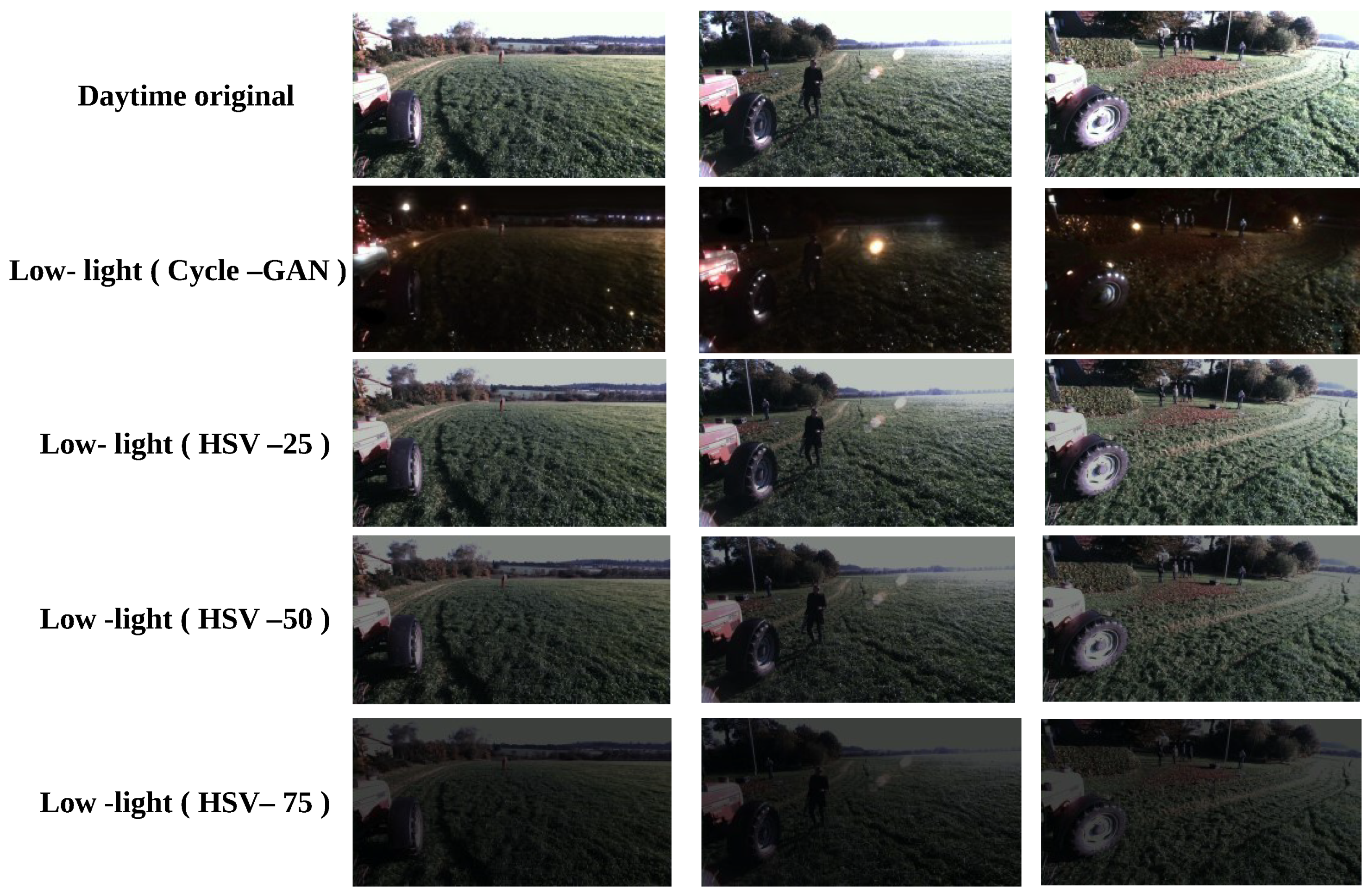
In this work, two methods are chosen to augment the dataset with low-light RGB images. The first one is the Cycle-GAN [6] which designed cyclic consistency losses to achieve style transformation with unpaired training datasets. This learning-based network is used to generate virtual nighttime images in experiments. For a better fidelity, both daytime and nighttime images from the large-scale dataset BDD100K [39] are applied to train the network, as shown in Figure 3.

Additionally, RGB images are converted into the HSV color space and adjust the brightness channel to generate dim light images. This method can avoid the problem of an unreal light spot learned by the Cycle-GAN from dataset BDD100K [39], but the images show low similarity to the real nighttime scenario. Samples of generated low-light images are shown in Figure 4, where HSV-25 means that the brightness of the image is reduced by $25\%$, and the same annotation applies to HSV-50 and HSV-75.

3.2. Generation of 3D Pedestrian Labels

Annotation for multi-sensor data is an extremely tedious task. It requires human experts with a lot of experience to accurately identify all the related LiDAR points which are corresponding to objects in the image. In this work, a semi-automatic annotation method is provided for a 3D perception task. First, a pinch of images are manually annotated with 2D bounding box labels and used to fine-tune a 2D detection network to annotate the rest images. The detection errors are only a few and revised by human experts. Second, LiDAR points are projected onto the image plane and the portion covered 2D bounding boxes is cropped. For the cropped points, the ground points are further removed and clustering based on Euclidean distance is conducted to find points on the pedestrian. Third, a 3D cylinder is generated according to the clustered LiDAR points. In comparison with a 3D bounding box, which is represented by its center, width, length, height, and yaw angle, the 3D cylinder is identified only by its center, radius, and height. Thus, the 3D cylinder label has fewer parameters than a cube which eases the regression task by the network. In the above annotation procedure, the 2D box provides a coarse lateral position for the object, which is key to the 3D label generation. By employing the semi-automation of 2D labels, the entire annotation process can be accelerated and thus the annotation work can be kept at a low labor and low time cost.

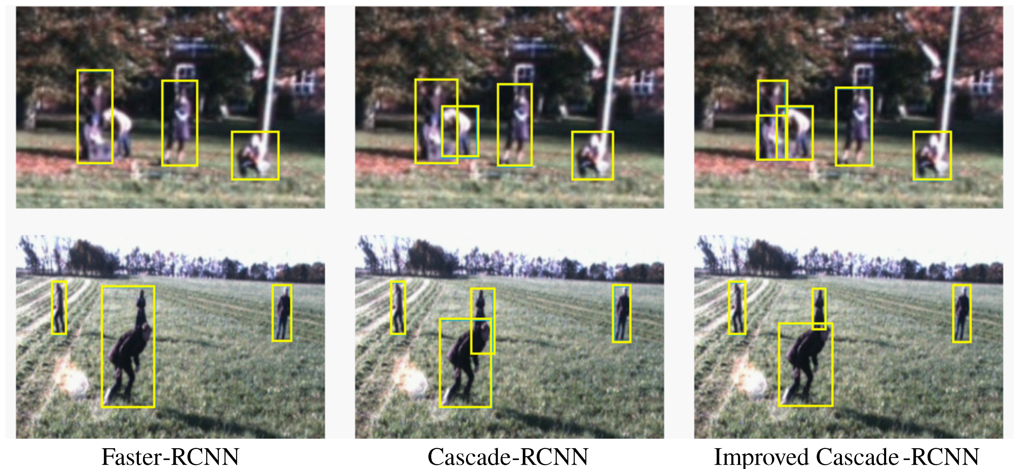
As aforementioned, a pinch of filtered images are firstly annotated by the open-source tool LabelImg [40], which is a graphical image annotation tool for labeling images with 2D bounding boxes and saving annotations files in PASCAL VOC, YOLO, or CreateML formats. The images are further divided into subsets with 2000 for training, 250 for validation, and 250 for testing. The fine-tuned network is the improved Cascade-RCNN [41] which employs the HRNet [42] as a substitute of the default backbone and modifies the anchor size by K-Means clustering [43] according to the distribution of 2D labels. The network is implemented by PyTorch. The epoch number is set to 24. Other training details are referred to Cascade-RCNN [41]. The ablation experiments on 2D detection demonstrate that the used network performs superior to both the Faster-RCNN [44] and the original Cascade-RCNN [41] on average precision (AP), as shown in

Table 1. Comparison of 2D detection results on three metrics: Mean AP (mAP), AP with a threshold of 0.5 and 0.7, respectively (AP-0.5, AP-0.7). The best values are displayed in bold.

Methods	Bbox-mAP $(\uparrow )$	Bbox-AP-0.5 $(\uparrow )$	Bbox-AP-0.75 $(\uparrow )$
Faster-RCNN [44]	0.416	0.596	0.421
Cascade-RCNN [41]	0.524	0.704	0.562
Proposed (+HRNet)	0.556	0.729	0.590
Proposed (+modified anchor)	0.528	0.708	0.569
Proposed (+HRNet+modified anchor)	0.558	0.733	0.593

and Figure 5. Thus, it is more suitable as an automatic annotation tools.

In the next step, 3D cylinder labels of each image are generated according to the LiDAR points and 2D labels are obtained. The ground points are firstly filtered by the RANSAC algorithm [45]. Thereafter, the remaining points are projected into a camera coordinate system, and those enclosed by the 2D box are kept. The enclosed point cloud is further clustered by the DBSCAN algorithm [46] to remove noise points in the background. Since LiDAR points on a pedestrian is relatively sparse in the dataset, the points may not completely cover the body surface. Therefore, the size of a corresponding point cluster may not be consistent with the the spatial size of the pedestrian.

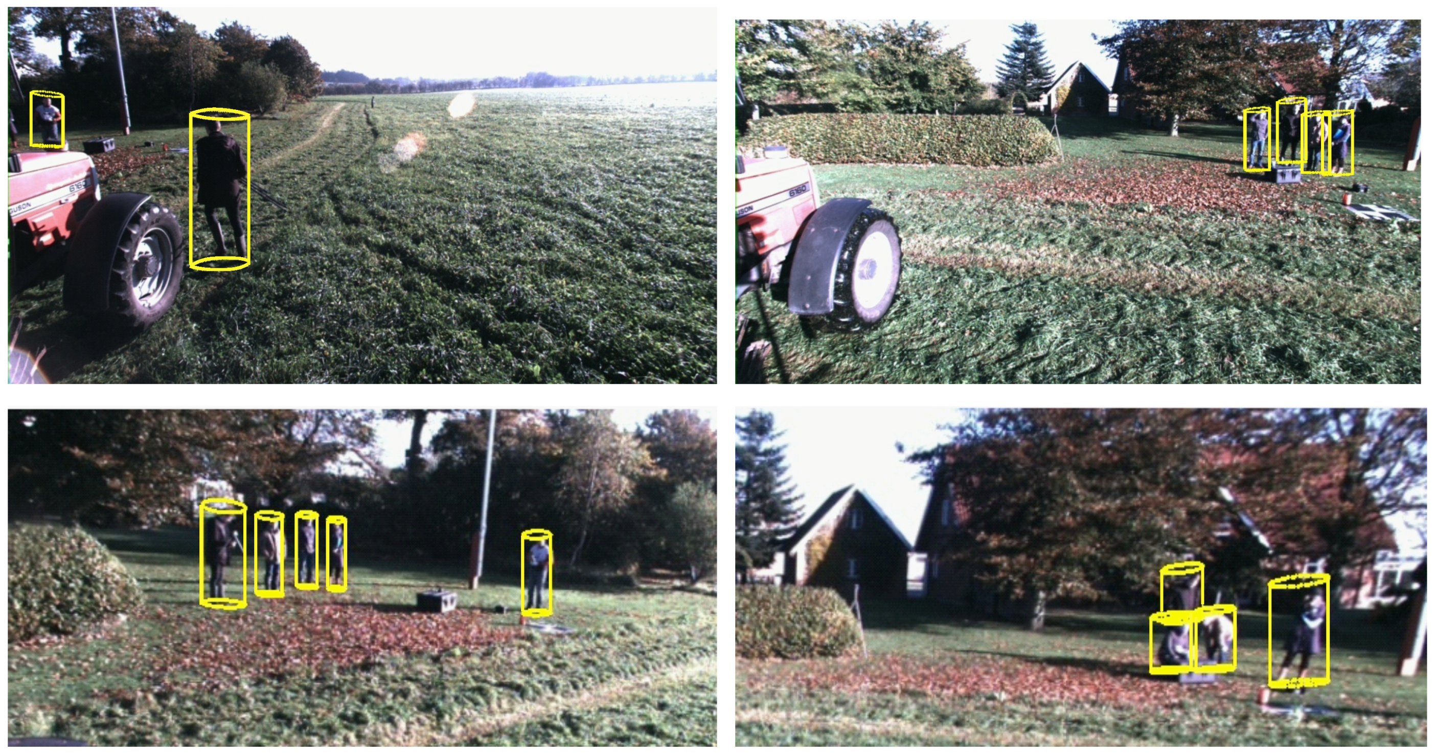
Hence, an additional size correction procedure is implemented. First, the average depth of LiDAR points and the 2D box center are used to jointly determine the location of a 3D cylinder in the camera coordinate system. The cylinder is initialized with the smallest pedestrian size (similar to a child) in the dataset. After that, the center coordinates, the height, and the radius of the cylinder are adjusted to gradually increase its size, until the projected shape of the cylinder is inscribed in the corresponding 2D bounding box. The final cylinder is the 3D label of the pedestrian, with samples shown in Figure 6.

After data preparation, the FieldSafePedestrian dataset totally consists of 48,120 data pairs of synchronized RGB image, FIR image, and LiDAR point cloud frame. Therein, 17,090 pairs contain positive images and have corresponding annotation files, and a total of 30,336 pedestrians in sitting, lying, and standing postures are marked with 3D cylinder labels. Most pedestrians occupy a 20–80 pixel height and within the range of 5–40 m from the camera. Finally, the dataset is augmented by aforementioned methods of Cycle-GAN, HSV-25, HSV-50, and HSV-72. Thus, the dataset is increased by a factor of $\times 4$ by adding the low-light images.

4. Methods

The Dual-Input Depth-Guided Dynamic-Depthwise-Dilated Fusion network (D5F) is proposed based on the prior work [30]. This new network strives to fuse the information from both FIR and RGB images to perform 3D pedestrian detection, which can lead to a more robust and accurate solution based on the advantage of rich RGB semantics and strong resistance to illumination changes by far-infrared sensing in a dark agricultural operation environment. The entire network consists of a depth estimation module, a data fusion module, a depth-guided dynamic local convolutional module, and a detection head, as shown in Figure 1. The contributions come mainly in following aspects:

• The depth map of RGB image is predicted by the depth estimation module, and assists the pixel alignment between RGB and FIR image thus building the concatenated channels for feature extraction network;
• The 3D cube is replaced by the 3D cylinder as the network output, which reduces regression parameters of the network and is conducive to its learning;
• Extensive experiments are conducted on the FieldSafePedestrian dataset for 3D cylinder detection, and demonstrates the efficacy of the improved network in comparison with other state-of-the-art methods.

4.1. Depth Estimation Module

The depth estimation module needs to output the pixel-wise depth value, which poses high requirements on the feature extractor. The depth estimation module is implemented based on the BTS network [13], which is selected according to experimental results in Section 5.1. This network includes a pyramid structure based on the dilated convolution. In each pyramid layer, a different dilated convolution rate is assigned to the convolution operation. Information from different receptive fields can be effectively fused in the network to extract multi-scale features.

The network estimates depth map of monocular images and is learned with supervision by LiDAR points. The obtained depth map is applied in two aspects in the proposed D5F. On one hand, the depth value assists the registration of FIR and monocular images, which can then be fused as heterogeneous sensing signal channels. On the other hand, the predicted depth map can provide spatial information which is useful for guiding the 3D perception task in the depth guidance module.

4.2. Data Fusion Module

The FIR camera senses far-infrared rays from the environment, and interprets the ray intensity as the pixel value of a gray image. FIR sensors are not sensitive to the sunlight and thus is suitable for detecting pedestrians in low-light environments. In order to combine advantages of both types of sensing information, alignment between the FIR and RGB image is conducted, which are merged as network input to improve the detection robustness.

Since both the perspective and field of view differ between the monocular RGB camera and FIR camera, and the depths corresponding to image pixels are variant, the fixed transform matrix such as the homography cannot be directly applied to the data registration. In this work, the depth information obtained by the depth estimation module in Section 4.1 is used to assist the alignment between the RGB and FIR image.

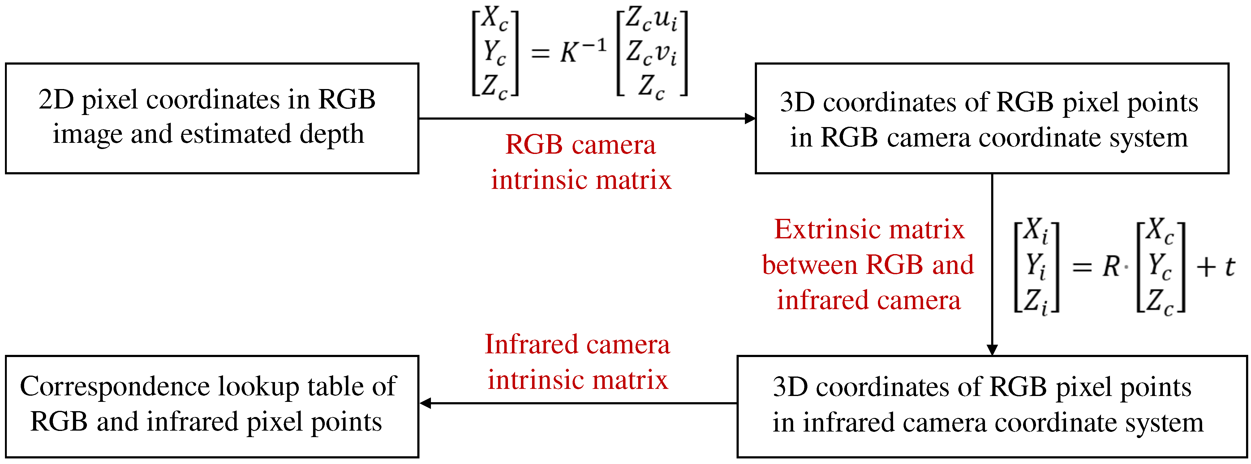
The alignment process is shown in Figure 7. According to the estimated depth map, for each RGB pixel, a 3D point in the RGB camera coordinate system can be obtained. The 3D point is further transformed into the FIR camera coordinate system based on the extrinsic parameters by the sensor setup. By projecting the 3D point in the FIR image plane, the associated pixel in the FIR image is obtained. In this way, a pixel-to-pixel association between the RGB and FIR image is established. Data registration and data fusion can be completed through the corresponding relationship.

4.3. Depth Guidance Module

The D5F network utilizes a deep guidance module to extract deep features respectively by two backbone networks, represented as the feature extraction network and the convolution kernel generation network. The first backbone uses the concatenated image channels as the network input and infers the feature map ${\mathbf{F}}_1$ and the learned weights $A_1$, $A_2$, $A_3$ for different dilated convolution rates. The feature map ${\mathbf{F}}_1$ also flows into the shift pooling module [47] which replaces the convolution process by the shift operation of feature map. Thus, the information fusion of the feature map in different spatial and channel dimensions can be obtained by a mean calculation (shown in Figure 8). The feature map of the shift pooling is denoted as ${\mathbf{F}}_3$.

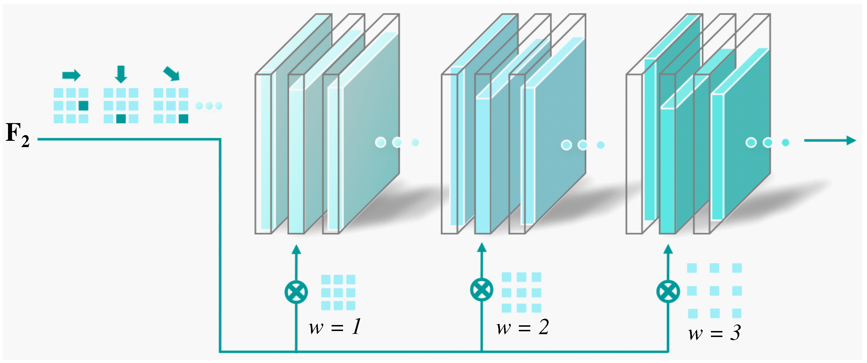
The second backbone uses the estimated depth map as input and yields the feature map ${\mathbf{F}}_2$. The feature map ${\mathbf{F}}_2$ is shifted according to the shift coordinates defined as $(g_i,g_j)$ with $g_i,g_j\in \left(int\right)[1-k/2,k/2-1]$, where $int$ is a rounding operation and k is the kernel size of feature extraction network. The shift coordinates actually determine the shift mode of the feature map. Three different modes with three dilated convolution rates are selected to shift ${\mathbf{F}}_2$, which leads to nine different shift results (Figure 9).

The shifted feature maps are further weighted by the learned parameters $A_1$, $A_2$, $A_3$, with each corresponding to one dilated convolution rate (Figure 1). Weighted features are summed as ${\mathbf{F}}_4$ Equation (3). An element-wise dot product between ${\mathbf{F}}_4$ and the output feature ${\mathbf{F}}_3$ of the shift pooling module is calculated to yield the feature map ${\mathbf{F}}_5$ Equation (4), which is fed into the classification and regression head.

$${\mathbf{F}}_4=\sum _r{A}_r·\sum _{g_i,g_j}{\mathbf{F}}_2^{\left(g_i\ast r,g_j\ast r\right)},$$

(3)

$${\mathbf{F}}_5=\frac{1}{d·k·k}·{\mathbf{F}}_3\odot {\mathbf{F}}_4,$$

(4)

where $A_r$ refers to the weight corresponding to one dilated convolution rate and learned from the feature extraction network, and d denotes the maximum dilation rate.

In the depth guidance module, since depth values depend on the observed scene, the weights of dilated convolution filters are dynamically estimated by the depth map. Filters of different dilated convolution rates also provide various perception fields. Along with the multiple shift modes, information from different spatial and channel dimensions can be effectively extracted from the depth map.

4.4. Detection Head

Similar to the framework of M3D-RPN [25], the score s of a detected pedestrian along with its 2D and 3D anchor is regressed by a series of $1\times 1$ convolutional layers. The 2D anchor is denoted by a bounding box with center $(x_{2d},y_{2d})$ and size $(w_{2d},h_{2d})$. However, for the 3D anchor, a cylinder is chosen to replace the cube used by M3D-RPN. Thus, the 3D anchor is represented by its spatial center $(x_{3d},y_{3d},z_{3d})$, the radius $r_{3d}$, and the height $h_{3d}$. Compared to cubes, the cylinder has less degrees of freedom, which is more conducive to network learning.

4.5. Multi-Task Loss

The proposed network is trained by a multi-task loss for both depth map generation and 3D cylinder detection. Respectively, the depth map generation network is trained with a loss Equation (5) as the combination of the variance and a weighted squared mean of the depth error in log space.

$$\left\{\begin{array}{cccc}\hfill & {\ell }_{depth}\hfill & \hfill =& \frac{1}{T}\sum _{i=0}^T{g}_i^2-{\left(\frac{1}{T}\sum _{i=0}^T{g}_i\right)}^2+\left(1-\lambda \right){\left(\frac{1}{T}\sum _{i=0}^T{g}_i\right)}^2\hfill \\ \hfill & g_i\hfill & \hfill =& \log \widetilde{d_i}-\log d_i\hfill \end{array}\right.,$$

(5)

where $\widetilde{d_i}$ is the predicted depth value of pixel i while $d_i$ stands for its ground truth. The hyper-parameter $\lambda$ is to balance between minimizing the variance of error and its mean, so that the network can better focus on the details of scene depth and less affected by the outlier values. In the experiment, $\lambda$ is set to 0.5. The number T denotes the total pixels with valid ground truth values.

In 3D detection, the loss is defined in Equation (6), including an entropy loss for classification and two smooth-L1 losses for parameter regression.

$$\left\{\begin{array}{cccc}\hfill & {\ell }_{total}\hfill & \hfill =& {\left(1-S_t\right)}^m\left({\ell }_{class}+{\ell }_{2d}+{\ell }_{3d}\right)\hfill \\ \hfill & {\ell }_{class}\hfill & \hfill =& -\log \left(S_t\right)\hfill \\ \hfill & {\ell }_{2d}\hfill & \hfill =& {\mathrm{SmoothL}}_1\left({\left[x_{2d},y_{2d},w_{2d},h_{2d}\right]}_{gt}^{\top },{\left[x_{2d},y_{2d},w_{2d},h_{2d}\right]}_{det}^{\top }\right)\hfill \\ \hfill & {\ell }_{3d}\hfill & \hfill =& {\mathrm{SmoothL}}_1\left({\left[x_{3d},y_{3d},z_{3d},r_{3d},h_{3d}\right]}_{gt}^{\top },{\left[x_{3d},y_{3d},z_{3d},r_{3d},h_{3d}\right]}_{det}^{\top }\right)\hfill \end{array}\right.,$$

(6)

where $S_t$ denotes the classification score and m is a hyper-parameter. Subscript ${[·]}_{det}$ indicates the predicted parameter for detection bounding box while ${[·]}_{gt}$ indicates its groundtruth.

5. Experimental Results

In the proposed framework, experiments are designed to accomplish two tasks, depth estimation and 3D pedestrian detection. All 48,120 data pairs of FieldSafePedestrian are divided into three parts, 80% for training, 10% for validation, and 10% for testing.

5.1. Experiments on Depth Estimation Module

The quality of estimated depth map is essential to both the alignment between RGB and FIR images and the generated filters in the depth guidance module. To implement the depth estimation module, here two supervised monocular depth estimation networks are compared, i.e., the BTS [13] and DORN [12]. Their performance is tested by experiments on daytime and low-light (generated by Cycle-GAN, HSV-25, HSV-50, and HSV-75) images in the FieldSafePedestrian dataset. Implementation and training details can be found in their original work [12,13].

For supervised training of depth estimation network, the groundtruth of each image is elaborated after data preparation in Section 3.1. The associated LiDAR points are projected to the RGB image plane according to the calibration parameters. The projected image (shown in Figure 10) can be considered as a sparse matrix whose size is $1024\times 544$ and equal to the RGB image. In this matrix, only pixels of projected LiDAR points are assigned with their depth values, while other pixels are considered as empty (with 0 value).

Referring to the evaluation protocol in [12], the metrics are absolute relative error (Abs_Rel) and Root Mean Squared Error (RMSE), formulated as:

$$\mathrm{Abs}\_\mathrm{Rel}=\frac{1}{T}\sum _{\tilde{d}\in T}\left(\left|\tilde{d}-d\right|d\right),$$

(7)

$$\mathrm{RMSE}=\sum _{\tilde{d}\in T}\sqrt{{∥\tilde{d}-d∥}^2},$$

(8)

where $\tilde{d}$ is the predicted depth map and d is its ground truth. T denotes the total pixel number.

The quantitative experimental results are shown in

Table 2. Results of monocular depth estimation.

Approach	Abs Rel $(\downarrow )$	RMSE $(\downarrow )$
DORN (day)	0.192	0.320
DORN (night)	0.390	0.493
BTS (day)	0.151	0.229
BTS (night)	0.306	0.395

. Compared with daytime test results, both approaches suffer from an increase of Abs_Rel and RMSE on low-light image testing, due to reduced environmental semantic information by lower illumination. However, the BTS still outperforms the DORN on various image qualities, which can be ascribed to two points. First, the BTS employs an improved feature extractor and fuses feature maps at different resolutions in the output layer of the network. Second, the BTS also utilizes a local plane guidance module to assist the depth estimation as well as to speed up the learning convergence. Qualitative results are shown in Figure 11, where the BTS shows superior performance in distinguishing the far away houses and sky areas. Based on the test results, BTS is chosen as the depth estimation module in the proposed network to conduct further experiments.

5.2. Experiments on 3D Object Detection

For detection evaluation, the protocol follows the NuScenes [35] and the BEV-IOU and the center distance are chosen as metrics, which provide complementary information to each other. For the first one, both the predicted cylinder and its groundtruth are projected on the ground plane and their intersection over the union ratio is calculated in the bird’s eye view. The second one is directly measured by the Euclidean distance between the centers of predicted 3D cylinder and its groundtruth. For quantitative evaluation, the threshold of BEV-IOU is set to 0.1. The thresholds of center distance are set to 0.5, 1, and 2 (meter), respectively, and their mean precision is also calculated, which is the same as in [35]. In addition, for all detected positive samples (within 1 m of center distance), reported results are the Mean Absolute Error (MAE) in depth direction (along the light ray from object center to the sensor) and its tangential direction and the MAE of both the radius and height of the cylinder.

Similarly to Section 5.1, experiments are conducted on the FieldSafePedestrian dataset. In this dataset, annotated pedestrians are divided into three difficulty levels according to their 2D bounding box size, denoted as hard (less then 25 pixels), moderate (25–40 pixels), and easy (more than 40 pixels). Thus, the average precision is calculated for each level. The D5F network is also implemented by the PyTorch framework and trained on an Nvidia 2080Ti GPU. The used optimizer is the Stochastic Gradient Descent (SGD), with a momentum of 0.9 and a weight decay of 0.0005. A “poly” learning rate is utilized, in which the base learning rate is set to 0.01 and the power to 0.9. The iteration number is set to 40,000. Both the annotated datasets and codes of the D5F approach will be available online (https://github.com/tjiiv-cprg/3D-Pedestrian-Detection-in-Farmland, accessed on 22 July 2021).

5.2.1. Ablation Studies

To explore the proposed network performance with multi-modal data registration as well as on various illumination conditions, ablation studies are conducted in this experiment. Here two versions of proposed approach are prepared: D5F-RF and D5F-DF. The former utilizes the dynamic data registration between RGB and FIR images by the estimated depth map proposed in this approach while the latter utilizes a fixed transform matrix (estimated by alignment at the first frame) between RGB and FIR cameras to direct fuse both image types. Test results of both versions are shown in

Table 3. Average precision in terms of center distance for three difficulty levels ($D_{easy}^c$, $D_{mod}^c$, and $D_{hard}^c$).

Approach	${\mathit{D}}_{\mathbf{easy}}^{\mathit{c}}(\uparrow )$	${\mathit{D}}_{\mathbf{mod}}^{\mathit{c}}(\uparrow )$	${\mathit{D}}_{\mathbf{hard}}^{\mathit{c}}(\uparrow )$
D5F-DF	10.97%	9.96%	8.86%
D5F-RF	15.91%	13.51%	11.95%

,

Table 4. Average precision in terms of BEV-IOU for three difficulty levels (BEV-IOU${}_{easy}$, BEV-IOU${}_{mod}$, and BEV-IOU${}_{hard}$).

Approach	BEV-IOU${}_{\mathbf{easy}}(\uparrow )$	BEV-IOU${}_{\mathbf{mod}}(\uparrow )$	BEV-IOU${}_{\mathbf{hard}}(\uparrow )$
D5F-DF	8.21%	6.48%	5.29%
D5F-RF	13.38%	11.35%	8.83%

and

Table 5. MAE of radius (R), height (H), and location in depth ($D_{dep}$) and tangential direction ($D_{tang}$) of predicted cylinder. Errors are measured in meters.

Approach	${\mathit{D}}_{\mathbf{dep}}(\downarrow )$	${\mathit{D}}_{\mathbf{tang}}(\downarrow )$	$\mathit{R}(\downarrow )$	$\mathit{H}(\downarrow )$
D5F-DF	0.763	0.445	0.074	0.079
D5F-RF	0.466	0.296	0.038	0.041

.

Obviously, by adding the data registration module, the D5F-RF significantly outperforms the D5F-DF, which demonstrates that dynamic data registration by estimated depth maps indeed improves the alignment accuracy between RGB and FIR images. Assuming that the agricultural machinery drives on bumpy field roads, the vibration and noise can lead to minor changes of extrinsic parameters of the sensor setup. However, the guided image alignment is dynamically conducted for each individual frame, which reduces the impact of data misalignment due to changes in external parameters. Thus, the proposed dynamic image alignment approach shows robustness to vibrations.

Qualitative results are shown in Figure 12. It can be seen that on both daytime and nighttime images, with the help of data registration, the D5F-RF maintains a higher detection precision than the D5F-DF, which further verifies the necessity of dynamic alignment between RGB and FIR images in the fusion-based detection approach.

5.2.2. Comparison with State-of-the-Arts

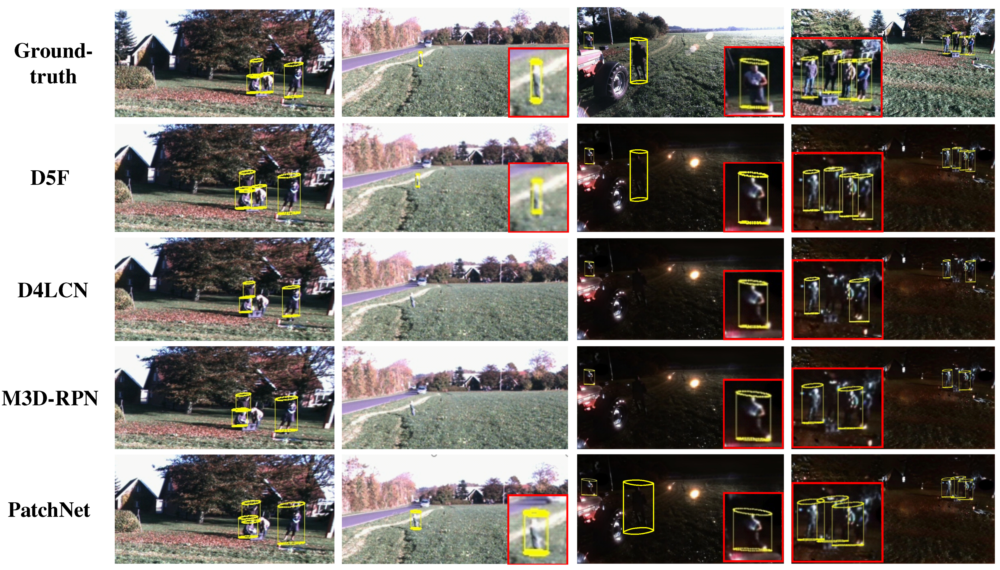
For the experiment, the proposed D5F is compared with three state-of-the-art 3D pedestrian detection approaches, the D4LCN [30], the M3D-RPN [25], and the PatchNet [29]. The D4LCN regresses object parameters based on depth estimations but only with RGB images. The M3D-RPN makes predictions directly on learned anchor priors. The PatchNet learns pseudo LiDAR points and interpret them as images. For fairness, the 3D anchor and regression parameters are modified in above networks to adapt them to the annotation setup. All compared approaches are trained on the FieldSafePedestrian dataset. To better investigate the performance of compared approaches in different working conditions, the detection results on the daytime and nighttime images are sorted. The test results for each metric are shown in

Table 6. Average precision in terms of center distance for three difficulty levels ($D_{easy}^c$, $D_{mod}^c$, and $D_{hard}^c$). The best values are displayed in bold.

Approach	${\mathit{D}}_{\mathbf{easy}}^{\mathit{c}}(\uparrow )$	${\mathit{D}}_{\mathbf{mod}}^{\mathit{c}}(\uparrow )$	${\mathit{D}}_{\mathbf{hard}}^{\mathit{c}}(\uparrow )$
PatchNet (day)	19.85%	15.84%	15.36%
M3D-RPN (day)	14.63%	11.76%	9.81%
D4LCN (day)	16.96%	13.68%	11.86%
D5F (day)	19.98%	16.32%	14.93%
PatchNet (night)	9.68%	8.47%	6.88%
M3D-RPN (night)	6.14%	5.97%	3.97%
D4LCN (night)	8.55%	7.39%	5.34%
D5F (night)	11.84%	10.69%	8.97%

,

Table 7. Average precision in terms of BEV-IOU for three difficulty levels (BEV-IOU${}_{easy}$, BEV-IOU${}_{mod}$, and BEV-IOU${}_{hard}$). The best values are displayed in bold.

Approach	BEV-IOU${}_{\mathbf{easy}}(\uparrow )$	BEV-IOU${}_{\mathbf{mod}}(\uparrow )$	BEV-IOU${}_{\mathbf{hard}}(\uparrow )$
PatchNet (day)	13.69%	11.83%	9.94%
M3D-RPN (day)	11.52%	9.98%	8.69%
D4LCN (day)	14.68%	12.74%	10.42%
D5F (day)	17.29%	14.86%	11.08%
PatchNet (night)	6.96%	5.24%	3.47%
M3D-RPN (night)	4.26%	3.62%	2.32%
D4LCN (night)	6.42%	4.29%	3.88%
D5F (night)	9.46%	7.84%	6.57%

and

Table 8. MAE of radius (R), height (H), and location in depth ($D_{dep}$) and tangential direction ($D_{tang}$) of predicted cylinder by compared approaches. Errors are measured in meters. The best values are displayed in bold.

Approach	${\mathit{D}}_{\mathbf{dep}}(\downarrow )$	${\mathit{D}}_{\mathbf{tang}}(\downarrow )$	$\mathit{R}(\downarrow )$	$\mathit{H}(\downarrow )$
PatchNet (day)	0.596	0.225	0.174	0.124
M3D-RPN (day)	0.752	0.321	0.068	0.078
D4LCN (day)	0.568	0.298	0.029	0.032
D5F (day)	0.430	0.268	0.009	0.011
PatchNet (night)	0.783	0.388	0.396	0.315
M3D-RPN (night)	0.895	0.549	0.091	0.105
D4LCN (night)	0.841	0.510	0.089	0.096
D5F (night)	0.502	0.324	0.066	0.069

.

As can be seen, all compared approaches achieve high precision on daytime images. The M3D-RPN performs inferior to other approaches on all metrics. Since the M3D-RPN is an anchor-based approach, it strongly relies on the priors learned by its anchors. Such a method is not well adapted to scenes with great variations such as the agricultural field. In comparison, the other three methods employ depth maps to assist the object detection, thus achieving an improved precision by better scene adaptability. When choosing the center distance as the criterion, the D5F performs the best on both easy and moderate levels, but with a minor gap of 0.4% to the PatchNet on the hard level. That means the PatchNet performs slightly better than the D5F network on the distance prediction for distant and small objects. It can be owed to the fact that the pseudo point cloud utilized in the PatchNet is optimally learned while the D5F network employs an off-the-shelf depth estimation module. Thus, the regressed depth map by D5F suffers from a sub-optimality in the entire architecture. However, on the BEV-IOU metric, the D5F performs the best on all difficulty levels, which implies the D5F outperforms the PatchNet on size prediction for pedestrians, as shown in the MAE results (Table 8) and proven by the qualitative results (Figure 13). Considering that the agricultural machinery commonly drive at a low speed, more attention should be given to the safety of pedestrians at a close and medium distance, making the D5F approach more applicable.

When testing on low-light images, for all compared approaches, large brightness reduction leads to a low average precision. From the results displayed in Table 6 and Table 7, the D5F yields the smallest performance degradation after illumination variation. In the D5F approach, RGB and FIR information are fused while other approaches solely rely on RGB images. This implies that the FIR image plays an important role in working conditions when target objects are difficult to distinguish from the background. With the help of FIR image, the D5F maintains a high detection rate in a low-light environment, which further proves the benefit of adding FIR information to the network.

Table 9. Inference time per frame of compared approaches.

Approach	Time per Frame (s)
PatchNet	0.42
M3D-RPN	0.16
D4LCN	0.21
D5F	0.24

reports the inference time per frame for compared approaches. Among them, the anchor-based M3D-RPN achieves the fastest speed of 160 ms per frame. By integrating depth estimation, the network is slowed down, e.g., the D4LCN takes about 50 ms. Another overhead of 30 ms is counted for data registration between RGB and FIR images. Thus, the D5F achieves 240 ms per frame, which is about 180 ms faster than the PatchNet. Note that, there is still space for accelerating the network inference, e.g., by network compression or distillation, which is planned in the future work.

Qualitative detection results on both daytime and low-light images are shown in Figure 13. It can be seen that when the target is small and far away from the camera, neither the M3D-RPN nor the D4LCN can detect the target. Only the D5F and PatchNet are able to detect small pedestrians, displayed in the third column of Figure 13. In nighttime conditions when target objects are difficult to distinguish from the background, only the PatchNet and D5F are able to maintain a high detection rate (last two columns of Figure 13). However, the predicted 3D cylinders by the PatchNet are significantly larger than the pedestrian body. Thus, the size accuracy of PatchNet is intuitively slightly worse than D5F.

6. Conclusions and Discussions

This paper addressed the driving safety of agricultural machinery in low-light working conditions by proposing the deep learning framework D5F, which significantly improved the robustness of 3D pedestrian detection in agricultural environment by fusing FIR and RGB images. Due to a lack of 3D pedestrian dataset in the agricultural environment, the new dataset “FieldSafePedestrian” is proposed with augmented nighttime images and is thus appropriate for evaluation under various illumination conditions. The annotation of this dataset was assisted by a semi-automatic approach and employed elaborately designed cylinder labels, which possessed reduced parameters to ease the model learning. Additionally, a depth-guided registration approach was proposed to address the dynamic alignment between RGB and FIR images. Its advantages over direct image fusion were validated through experiments on field images, with an accuracy increase of 3.9% and 4.5% in terms of center distance and BEV-IOU, respectively.

In future work, the potential of the proposed approach should be explored to generate more stable and accurate object detection results, e.g., by further employing attention mechanism for better feature extraction from low quality RGB images. Since the proposed dataset only consists of ordinary daytime and nighttime images, it will be augmented with more scenarios such as overexposure and adverse weathers. Current data is only captured by sensors installed on the front side of the tractor. A different sensor setup such as the on-board installation may provide an elevated view, in which the detection is supposed to improve, especially in crowded scenarios. This is also included in the future work.

References

1. Kragh, M.; Jørgensen, R.; Pedersen, H. Object Detection and Terrain Classification in Agricultural Fields Using 3D Lidar Data. In Proceedings of the International Conference on Computer Vision Systems, Copenhagen, Denmark, 6–9 July 2015; pp. 188–197. [Google Scholar]
2. Liu, H.; Zhang, L.; Shen, Y.; Zhang, J.; Wu, B. Real-time Pedestrian Detection in Orchard Based on Improved SSD. Trans. Chin. Soc. Agric. Mach. 2019, 50, 29–37. [Google Scholar]
3. Hamed, R.; Hassan, Z.; Hassan, M.; Gholamreza, A. A new DSWTS algorithm for real-time pedestrian detection in autonomous agricultural tractors as a computer vision system. Measurement 2016, 93, 126–134. [Google Scholar]
4. Mihçioğlu, M.; Alkar, A. Improving pedestrian safety using combined HOG and Haar partial detection in mobile systems. Traffic Inj. Prev. 2019, 20, 619–623. [Google Scholar] [CrossRef]
5. Kragh, M.; Christiansen, P.; Laursen, M. FieldSAFE: Dataset for obstacle detection in agriculture. Sensors 2017, 17, 2579. [Google Scholar] [CrossRef] [PubMed] [Green Version]
6. Zhu, J.; Park, T.; Isola, P.; Efros, A. Unpaired Image-To-Image Translation Using Cycle-Consistent Adversarial Networks. In Proceedings of the IEEE International Conference on Computer Vision, Venice, Italy, 22–29 October 2017; pp. 2223–2232. [Google Scholar]
7. Chen, Q.; Xie, Y.; Guo, S.; Bai, J.; Shu, Q. Sensing system of environmental perception technologies for driverless vehicle: A review of state of the art and challenges. Sensors Actuators A Phys. 2021, 319, 1–15. [Google Scholar] [CrossRef]
8. Eigen, D.; Puhrsch, C.; Fergus, R. Depth map prediction from a single image using a multi-scale deep network. In Proceedings of the International Conference on Neural Information Processing Systems, Copenhagen, Denmark, 6–9 July 2015; pp. 2366–2375. [Google Scholar]
9. Liu, F.; Shen, C.; Lin, G. Learning depth from single monocular images using deep convolutional neural fields. IEEE Trans. Pattern Anal. Mach. Intell. 2016, 38, 2024–2039. [Google Scholar] [CrossRef] [Green Version]
10. Li, B.; Shen, C.; Dai, Y. Depth and surface normal estimation from monocular images using regression on deep features and hierarchical CRFs. In Proceedings of the 2015 IEEE Conference on Computer Vision and Pattern Recognition (CVPR), Boston, MA, USA, 7–12 June 2015; pp. 1119–1127. [Google Scholar]
11. Iro, L.; Christian, R.; Vasileios, B. Deeper depth prediction with fully convolutional residual networks. In Proceedings of the 4th International Conference on 3D Vision, Stanford, CA, USA, 25–28 October 2016; pp. 239–248. [Google Scholar]
12. Fu, H.; Gong, M.; Wang, C.; Batmanghelich, K.; Tao, D. Deep ordinal regression network for monocular depth estimation. In Proceedings of the IEEE Conference on Computer Vision and Pattern Recognition (CVPR), Salt Lake City, UT, USA, 18–23 June 2018; pp. 2002–2011. [Google Scholar]
13. Lee, J.; Han, M.; Ko, D.; Suh, I. From big to small: Multi-scale local planar guidance for monocular depth estimation. arXiv 2020, arXiv:1907.10326. [Google Scholar]
14. Zhou, T.; Brown, M.; Snavely, N.; Lowe, D. Unsupervised learning of depth and egomotion from video. In Proceedings of the IEEE Conference on Computer Vision and Pattern Recognition (CVPR), Honolulu, HI, USA, 21–26 July 2017; pp. 6612–6619. [Google Scholar]
15. Yin, Z.; Shi, J. Geonet: Unsupervised learning of dense depth, optical flow and camera pose. In Proceedings of the IEEE/CVF Conference on Computer Vision and Pattern Recognition (CVPR), Salt Lake City, UT, USA, 18–23 June 2018; pp. 1983–1992. [Google Scholar]
16. Godard, C.; Aodha, O.; Firman, M.; Brostow, G. Digging into self-supervised monocular depth estimation. arXiv 2019, arXiv:1806.01260. [Google Scholar]
17. Chen, X.; Kundu, K.; Zhang, Z.; Ma, H.; Fidler, S.; Urtasun, R. Monocular 3D Object Detection for Autonomous Driving. In Proceedings of the IEEE Conference on Computer Vision and Pattern Recognition (CVPR), Las Vegas, NV, USA, 27–30 June 2016; pp. 2147–2156. [Google Scholar]
18. He, T.; Soatto, S. Mono3D++: Monocular 3D Vehicle Detection with Two-Scale 3D Hypotheses and Task Priors. In Proceedings of the AAAI Conference on Artificial Intelligence, Honolulu, HI, USA, 27 January–1 February 2019; pp. 8409–8416. [Google Scholar]
19. Chabot, F.; Chaouch, M.; Rabarisoa, J.; Teuliere, C.; Chateau, T. Deep MANTA: A Coarse-To-Fine Many-Task Network for Joint 2D and 3D Vehicle Analysis From Monocular Image. In Proceedings of the IEEE Conference on Computer Vision and Pattern Recognition (CVPR), Honolulu, HI, USA, 21–26 July 2017; pp. 2040–2049. [Google Scholar]
20. Manhardt, F.; Kehl, W.; Gaidon, A. ROI-10D: Monocular Lifting of 2D Detection to 6D Pose and Metric Shape. In Proceedings of the IEEE/CVF Conference on Computer Vision and Pattern Recognition (CVPR), Long Beach, CA, USA, 15–20 June 2019; pp. 2069–2078. [Google Scholar]
21. Liu, Z.; Wu, Z.; Toth, R. SMOKE: Single-Stage Monocular 3D Object Detection via Keypoint Estimation. In Proceedings of the IEEE/CVF Conference on Computer Vision and Pattern Recognition Workshops (CVPR), Seattle, WA, USA, 14–19 June 2020; pp. 996–997. [Google Scholar]
22. Zhou, X.; Wang, D.; Krähenbühl, P. Objects as Points. arXiv 2019, arXiv:1904.07850. [Google Scholar]
23. Li, P.; Zhao, H.; Liu, P.; Cao, F. RTM3D: Real-time monocular 3D detection from object keypoints for autonomous driving. arXiv 2020, arXiv:2001.03343. [Google Scholar]
24. Mousavian, A.; Anguelov, D.; Flynn, J.; Kosecka, J. 3D Bounding Box Estimation Using Deep Learning and Geometry. In Proceedings of the IEEE Conference on Computer Vision and Pattern Recognition (CVPR), Honolulu, HI, USA, 21–26 July 2017; pp. 7074–7082. [Google Scholar]
25. Brazil, G.; Liu, X. M3D-RPN: Monocular 3D Region Proposal Network for Object Detection. In Proceedings of the IEEE/CVF International Conference on Computer Vision, Long Beach, CA, USA, 16–20 June 2019; pp. 9287–9296. [Google Scholar]
26. Xu, B.; Chen, Z. Multi-Level Fusion Based 3D Object Detection From Monocular Images. In Proceedings of the IEEE Conference on Computer Vision and Pattern Recognition (CVPR), Salt Lake City, UT, USA, 18–23 June 2018; pp. 2345–2353. [Google Scholar]
27. Wang, Y.; Chao, W.; Garg, D.; Hariharan, B.; Campbell, M.; Weinberger, K. Pseudo-LiDAR From Visual Depth Estimation: Bridging the Gap in 3D Object Detection for Autonomous Driving. In Proceedings of the IEEE/CVF Conference on Computer Vision and Pattern Recognition (CVPR), Long Beach, CA, USA, 15–20 June 2019; pp. 8445–8453. [Google Scholar]
28. Qi, C.; Liu, W.; Wu, C.; Su, H.; Guibas, L. Frustum PointNets for 3D Object Detection From RGB-D Data. In Proceedings of the IEEE Conference on Computer Vision and Pattern Recognition (CVPR), Salt Lake City, UT, USA, 18–23 June 2018; pp. 918–927. [Google Scholar]
29. Ma, X.; Liu, S.; Xia, Z.; Zhang, H.; Zeng, X.; Ouyang, W. Rethinking pseudo-LiDAR representation. arXiv 2020, arXiv:2008.04582. [Google Scholar]
30. Ding, M.; Huo, Y.; Yi, H.; Wang, Z.; Shi, J.; Lu, Z.; Luo, P. Learning Depth-Guided Convolutions for Monocular 3D Object Detection. In Proceedings of the IEEE/CVF Conference on Computer Vision and Pattern Recognition (CVPR), Seattle, WA, USA, 13–19 June 2020; pp. 1000–1001. [Google Scholar]
31. Geiger, A.; Lenz, P.; Urtasun, R. Are we ready for autonomous driving? The KITTI vision benchmark suite. In Proceedings of the IEEE Conference on Computer Vision and Pattern Recognition (CVPR), Providence, RI, USA, 16–21 June 2012; pp. 3354–3361. [Google Scholar]
32. Hinterstoisser, S.; Lepetit, V.; Ilic, S.; Holzer, S.; Bradski, G. Model Based Training, Detection and Pose Estimation of Texture-Less 3D Objects in Heavily Cluttered Scenes. In Proceedings of the Asian Conference on Computer Vision, Daejeon, Korea, 5–9 November 2012; pp. 548–562. [Google Scholar]
33. Xiang, Y.; Schmidt, T.; Narayanan, V.; Fox, D. PoseCNN: A Convolutional Neural Network for 6D Object Pose Estimation in Cluttered Scenes. arXiv 2018, arXiv:1711.00199. [Google Scholar]
34. Song, X.; Wang, P.; Zhou, D.; Zhu, R.; Guan, C. ApolloCar3D: A Large 3D Car Instance Understanding Benchmark for Autonomous Driving. In Proceedings of the IEEE/CVF Conference on Computer Vision and Pattern Recognition (CVPR), Long Beach, CA, USA, 15–20 June 2019; pp. 5452–5462. [Google Scholar]
35. Caesar, H.; Bankiti, V.; Lang, A.H.; Vora, S.; Liong, V.E.; Xu, Q.; Krishnan, A.; Pan, Y.; Baldan, G.; Beijbom, O. nuScenes: A multimodal dataset for autonomous driving. arXiv 2019, arXiv:1903.11027. [Google Scholar]
36. Peynot, T.; Scheding, S.; Terho, S. The Marulan Data Sets: Multi-sensor Perception in a Natural Environment with Challenging Conditions. Int. J. Robot. Res. 2010, 29, 1602–1607. [Google Scholar] [CrossRef] [Green Version]
37. Pezzementi, Z.; Tabor, T.; Hu, P.; Chang, J.; Ramanan, D. Comparing Apples and Oranges: Off-Road Pedestrian Detection on the NREC Agricultural Person-Detection Dataset. arXiv 2017, arXiv:1707.07169. [Google Scholar]
38. Lowe, D. Distinctive Image Features from Scale-Invariant Keypoints. Int. J. Robot. Res. 2004, 60, 91–110. [Google Scholar] [CrossRef]
39. Yu, F.; Chen, H.; Wang, X.; Xian, W.; Chen, Y. BDD100K: A Diverse Driving Dataset for Heterogeneous Multitask Learning. In Proceedings of the IEEE/CVF Conference on Computer Vision and Pattern Recognition (CVPR), Seattle, WA, USA, 13–19 June 2020; pp. 2636–2645. [Google Scholar]
40. Tzuta, L. LabelImg. Git Code. 2015. Available online: https://github.com/tzutalin/labelImg (accessed on 22 July 2021).
41. Cai, Z.; Vasconcelos, N. Cascade R-CNN: High quality object detection and instance segmentation. IEEE Trans. Pattern Anal. Mach. Intell. 2019, 43, 1483–1498. [Google Scholar] [CrossRef] [PubMed] [Green Version]
42. Sun, R.; Zhao, Y.; Jiang, B.; Cheng, T.; Xiao, B. High-Resolution Representations for Labeling Pixels and Regions. arXiv 2019, arXiv:1904.04514. [Google Scholar]
43. MacQueen, J.B. Some methods for classification and analysis of multivariate observations. In Proceedings of the 5th Berkeley Symposium on Mathematical Statistics and Probability, Berkeley, CA, USA, 1967; pp. 281–297. Available online: https://projecteuclid.org/ebooks/berkeley-symposium-on-mathematical-statistics-and-probability/Proceedings%20of%20the%20Fifth%20Berkeley%20Symposium%20on%20Mathematical%20Statistics%20and%20Probability,%20Volume%201:%20Statistics/chapter/Some%20methods%20for%20classification%20and%20analysis%20of%20multivariate%20observations/bsmsp/1200512992 (accessed on 20 July 2021).
44. Ren, S.; He, K.; Girshick, R.; Sun, J. Faster R-CNN: Towards Real-Time Object Detection with Region Proposal Networks. arXiv 2015, arXiv:1506.01497. [Google Scholar] [CrossRef] [PubMed] [Green Version]
45. Fischler, M.A.; Bolles, R.C. Random sample consensus: A paradigm for model fitting with applications to image analysis and automated cartography. Commun. ACM 1981, 24, 381–395. [Google Scholar] [CrossRef]
46. Arlia, D.; Coppola, M. Experiments in Parallel Clustering with DBSCAN. In Proceedings of the International Euro-Par Conference, Manchester, UK, 28–31 August 2001. [Google Scholar]
47. Wu, B.; Wan, A.; Yue, X.; Jin, P.; Zhao, S.; Golmant, N.; Gholaminejad, A.; Gonzalez, J.; Keutzer, K. Shift: A Zero FLOP, Zero Parameter Alternative to Spatial Convolutions. arXiv 2020, arXiv:1711.08141. [Google Scholar]
Figure 1. The framework of 3D pedestrian detection in farmland. Dataset generation and pedestrian detection are included in this work. The FIR image pixels are aligned with RGB image pixels by the estimated depth map. Concatenated image channels and estimated depth map are respectively imported to convolution networks to extract deep semantic features, which are further fused to predict the 3D cylinder label of each pedestrian in the agricultural field.
Remotesensing 13 02896 g001
Figure 2. Matched feature points. The SIFT descriptor is utilized to conduct point matching and calculate the perspective transform matrix between the current frame and the template.
Remotesensing 13 02896 g002
Figure 3. The training and inferring phase of Cycle-GAN. The network is trained with daytime and nighttime images from BDD100K [39], and utilize the trained network to generate virtual nighttime images.
Remotesensing 13 02896 g003
Figure 4. Generation of low-light images. From top to bottom are images in daytime, generated images by Cycle-GAN, generated images by reducing brightness of 25%, 50%, and 75%, respectively.
Remotesensing 13 02896 g004
Figure 5. Examples of 2D detection results.
Remotesensing 13 02896 g005
Figure 6. 3D pedestrian labels and annotated image samples.
Remotesensing 13 02896 g006
Figure 7. Procedure of data registration between the RGB image and FIR image.
Remotesensing 13 02896 g007
Figure 8. Shift pooling module.
Remotesensing 13 02896 g008
Figure 9. Feature map shift.
Remotesensing 13 02896 g009
Figure 10. Projection of associated LiDAR points on the image plane. Projected points on the image plane are interpreted within a sparse matrix which presents the depth of each pixel value.
Remotesensing 13 02896 g010
Figure 11. Depth estimation results of monocular RGB images. The bottom area of depth maps by BTS and DORN are mostly with value 0 due to the blind area of LiDAR and label design. Areas with significant differences of depths are displayed within red boxes.
Remotesensing 13 02896 g011
Figure 12. Detection results of D5F-DF and D5F-RF on test images. Small objects are displayed in a zoomed red window.
Remotesensing 13 02896 g012
Figure 13. 3D pedestrian detection results on both daytime and nighttime images. Small objects are displayed in a zoomed red window (in the third column only the small pedestrian on the left image boundary is displayed).
Remotesensing 13 02896 g013