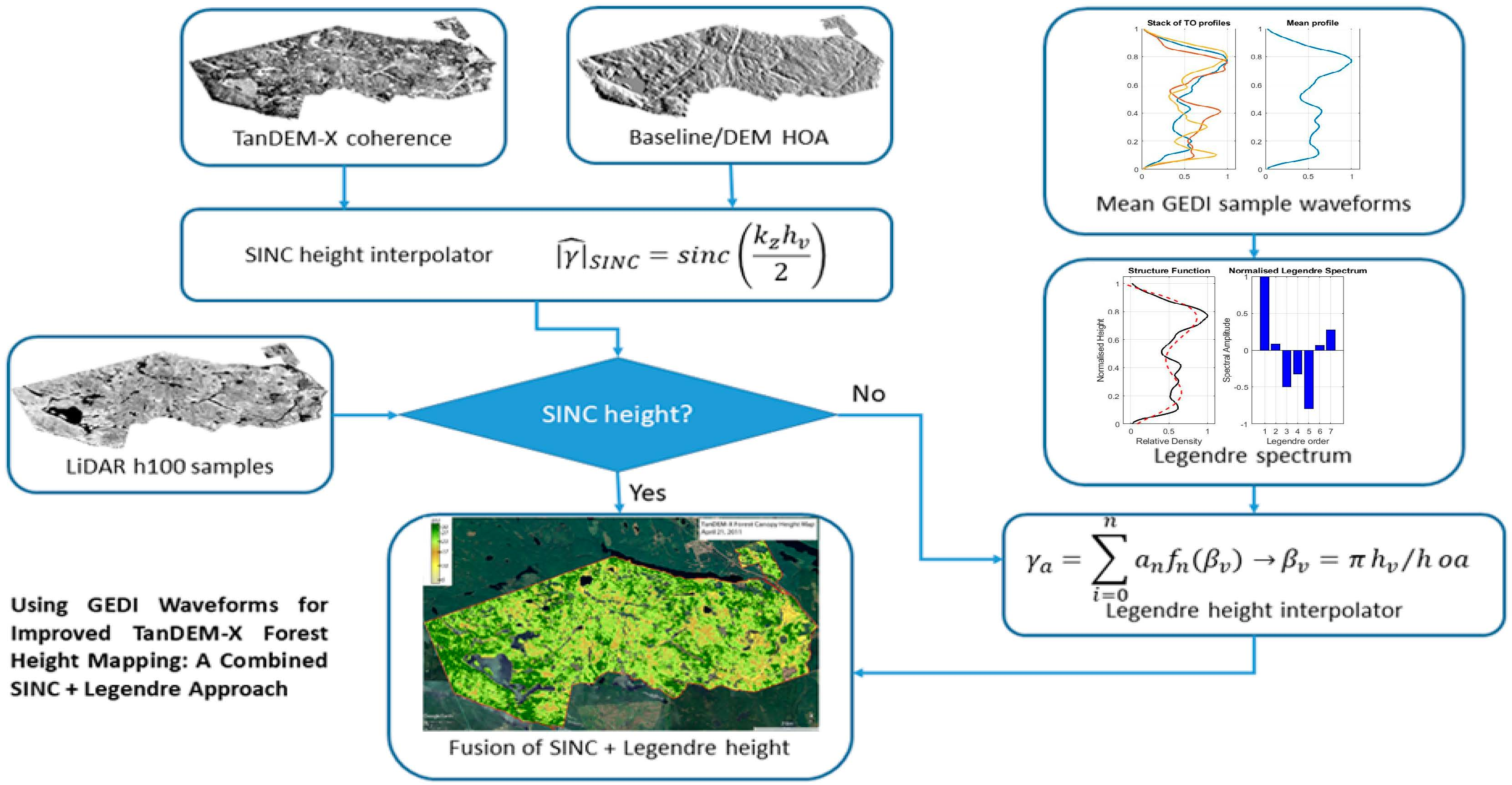
Using GEDI Waveforms for Improved TanDEM-X Forest Height Mapping: A Combined SINC + Legendre Approach

Abstract

In this paper, we consider a new method for forest canopy height estimation using TanDEM-X single-pass radar interferometry. We exploit available information from sample-based, space-borne LiDAR systems, such as the Global Ecosystem Dynamics Investigation (GEDI) sensor, which offers high-resolution vertical profiling of forest canopies. To respond to this, we have developed a new extended Fourier-Legendre series approach for fusing high-resolution (but sparsely spatially sampled) GEDI LiDAR waveforms with TanDEM-X radar interferometric data to improve wide-area and wall-to-wall estimation of forest canopy height. Our key methodological development is a fusion of the standard uniform assumption for the vertical structure function (the SINC function) with LiDAR vertical profiles using a Fourier-Legendre approach, which produces a convergent series of approximations of the LiDAR profiles matched to the interferometric baseline. Our results showed that in our test site, the Petawawa Research Forest, the SINC function is more accurate in areas with shorter canopy heights (<~27 m). In taller forests, the SINC approach underestimates forest canopy height, whereas the Legendre approach avails upon simulated GEDI forest structural vertical profiles to overcome SINC underestimation issues. Overall, the SINC + Legendre approach improved canopy height estimates (RMSE = 1.29 m) compared to the SINC approach (RMSE = 4.1 m).

1. Introduction

The capacity to derive wall-to-wall estimates of forest canopy height over large forest extents is a fundamental information need for many forest science, management, and policy applications. There is currently great interest in the capacity to improve wide-area forest canopy height estimates derived from TanDEM-X single-pass radar interferometry by focusing on forest height inversion modeling and by integrating data from the Global Ecosystem Dynamics Investigation (GEDI) full waveform LiDAR or radar tomography to estimate vertical forest profile functions [1,2,3,4,5]. Standard profile estimation functions, such as assuming a uniform vertical profile (the SINC approximation [6,7]) or exponential (as in the Random-Volume-Over-Ground (RVOG) model [8]) are often assumed to be inaccurate for complex forest environments with heterogeneous vertical structures. Whereas LiDAR provides the greatest vertical resolution, it has important differences from the radar in terms of viewing geometry [4], leading in particular to the strong influence of ground returns in open and lower biomass forests, while direct radar tomography has limitations in vertical resolution [5], but better mimics the sensing geometry of radar interferometers and so potentially provides a better balanced profile at the wavelength of the interferometer.

Key to both approaches, whether using LiDAR or radar tomography, is the question of how much vertical profile resolution is required for good height estimation from TanDEM-X? In this paper, we address this issue by proposing a novel Legendre series approach [9,10,11]. The first key point is that the requirements for vertical profile resolution do not depend solely on the profiling sensor itself (LiDAR or radar tomography). The interferometric baseline (more particularly, the product of the baseline and canopy height, or equivalently—the ratio of canopy height (h_v) to radar height-of-ambiguity (hoa)) is a key factor. For small baseline products (i.e. with a small h_v to hoa ratio), the actual vertical profile is irrelevant, regardless of how complicated the vertical structure of the canopy may be. In this scenario, the SINC model provides accurate height estimates [6]. It is only as this product of the baseline and canopy height increases that the radar interferometer becomes sensitive to changes in the vertical structure of the canopy. For sufficiently small h_v/hoa ratios, all trees appear uniform in terms of their vertical structure.

Secondly, the SINC approach has an important property as a lower bound. It provides the lowest possible estimate of canopy height for any given interferometric coherence and therefore plays an important role as a lower bound on canopy height estimates (and subsequently on derived quantities such as biomass). This is important because sometimes uncorrected coherence contributions can yield overestimated heights, even for the SINC model, in which case the use of higher resolution vertical profiles should be avoided. A SINC check of height in areas with point sampled LiDAR (i.e., GEDI) or tomographic data, where true height is known, can provide assurance that alternative approaches for applying vertical profiles are valid.

Given the aforementioned context, we posit that high-resolution vertical canopy profiles are only required for large baseline-canopy height products (i.e., with a large h_v to hoa ratio). Herein we propose a series approach to profile estimation and its use in radar interferometry. By employing a Fourier-Legendre series expansion of the vertical profile, we identify and rank those components required for a given height-baseline product. The low frequency components of the profile will always be dominant in modelling the response of the interferometer, while the higher spatial frequency components add incrementally smaller corrections, as required. Our objective is to demonstrate our approach by employing series expansions of simulated high-resolution GEDI LiDAR waveform profiles to improve canopy height estimates from TanDEM-X single-pass interferometric data.

2. Study Site and Data Preparation

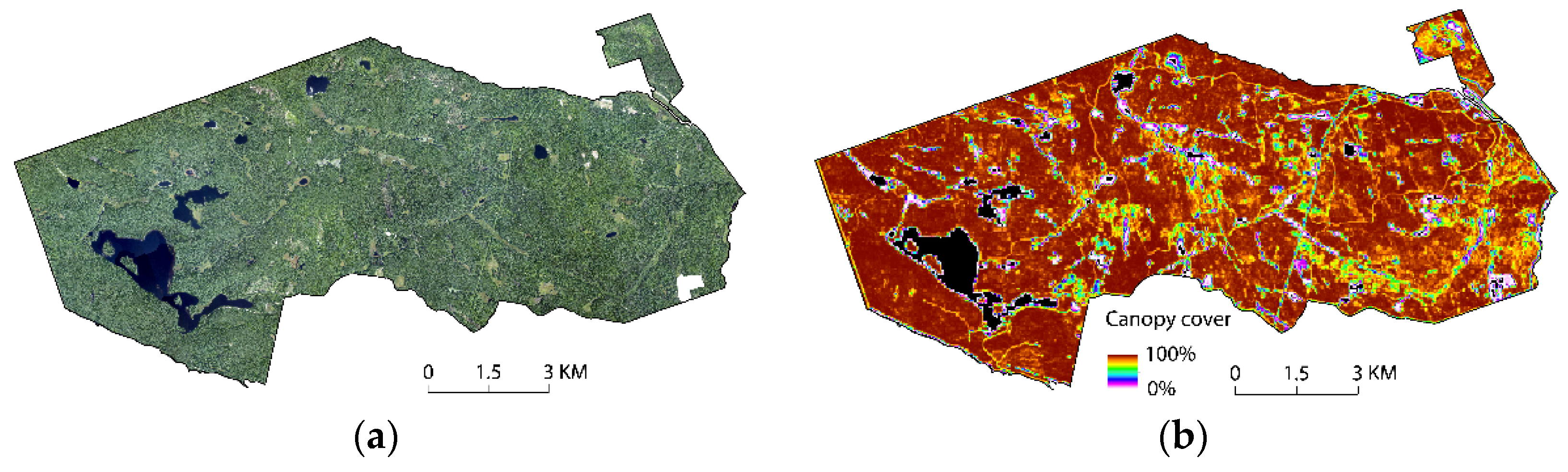
2.1. Study Site

The Petawawa Research Forest (PRF) was established in 1918 and is located approximately 160 km northwest of Ottawa, Canada, centered on 45.97°N and 77.50°W [12]. The PRF occupies approximately 100 km² of forested land and within the Great Lakes St. Lawrence Forest Region (Figure 1a). Forests in the PRF are dominated by mature temperate mixedwood stands (70% by area) with remaining stands being dominated primarily by hardwood (22%) or conifer (8%) species. Forests represent diverse forest structures as a function of their complex management histories, with a range of stand densities and canopy cover (Figure 1b). Mean canopy height is ~21 m, with maximum height ~42 m. The landscape is gently rolling with a median slope value ~4° and 90% of slopes less than 9°. The PRF has been the site of numerous operational and experimental remotely sensed data acquisitions [13] that have played a critical role in the development of enhanced forest inventories [14].

2.2. TanDEM-X Interferometric Data

A TanDEM-X Co-registered Single-look Slant-range Complex (CoSSC) image pair, collected over the PRF on 21 April 2011, was used for this study, courtesy of the German Aerospace Centre (DLR) as part of their science support program. The CoSSC data product has single polarization (HH) with a ground range resolution of 2.6 m and azimuth resolution of 3.3 m. The incidence angle at the scene centre is 42.6° and the hoa is nominally |43.9| m. The CoSSC image pair was initially processed and co-registered by the DLR to generate the interferogram in slant-range geometry. We estimated interferometric coherence with a 9 × 9 boxcar filter and performed coherence compensations to reduce the variance and bias [6]. The resulting slant-range coherence was terrain-corrected in UTM projection (Zone 18) with a pixel spacing of 25 m by using the ESA-SNAP software toolbox (https://step.esa.int/main/toolboxes/snap/, accessed on 19 January 2021).

2.3. Airborne Laser Scanning Data

Wall-to-wall discrete-return airborne laser scanning (ALS) data with an average point density of 10 points/m² (all returns), were acquired for the PRF in August 2012, using a LMS-Reigl Q680i. LAStools (http://rapidlasso.com/LAStools, accessed on 12 August 2020) was used to process ALS data to derive a Digital Elevation Model (DEM) and a Canopy Height Model (CHM) with a 2 m spatial resolution. The CHM was then used to derive an h100 raster, which is the mean of 100 tallest trees/hectare [15], determined by finding the maximum CHM height within a 5 × 5 filter window sliding across the CHM and resampling to a pixel size of 25 m. The h100 was used as an independent reference source for validating TanDEM-X forest canopy height estimates. For TanDEM-X height validation, gridcells that were < 2 m in the h100 were excluded, as the SINC model loses sensitivity at very low h_v to hoa ratios and greater errors would be expected from TanDEM-X height estimates in that range [7].

2.4. GEDI Data

GEDI data are comprised of 25 m footprints along eight ground tracks, spaced 60 m apart in the along-track direction and 600 m apart in the across-track direction. GEDI Level 1B geolocated waveform data acquired on 18 October 2019 [16] provided spatial coverage of the PRF and the majority of data passed the quality filtering standards [17]. For each valid GEDI footprint from this acquisition date, full waveform data were simulated from 2012 ALS data using the GEDI simulator [18], providing vertical profiles that were contemporaneous with the TanDEM-X data acquired in 2011.

2.5. Forest Inventory Data

An updated forest inventory was completed for the PRF circa 2018. A total of 4539 forest stands were manually delineated from aerial photography and assigned a suite of standard forest inventory attributes by a photointerpreter. Attributes included an estimate of vertical complexity, which indicates whether a forest stand is single-layer (SI), two-layer (TO, TU), multi-layer (MO, MU), or complex (CX), and which layer is the managed layer (O = overstorey, U = understorey) [19], with the majority (>85%) of stands and forest area classified as TO and CX. Our analysis was restricted to treed areas in the inventory.

3. Methods

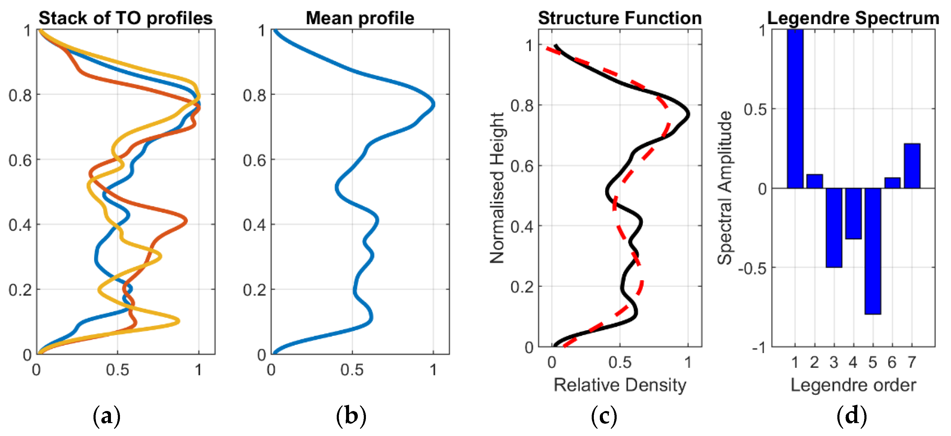
3.1. Radar Interferometry: Legendre Profiles

When an invertible model of the vegetation, such as the RVOG model [8] that contains a single attenuating layer over a surface, is employed, it gives the radar interferometric coherence some dependence on the (unknown) wave extinction in the canopy, a form of vertical structure. For a single baseline observation, the complex interferometric coherence observed for a random vertical distribution of scatterers can be written in a general form as shown in (1) [20,21,22]

$$\widehat{\gamma }=e^{i{k}_z{z}_0}\frac{{{\displaystyle \int }}_0^{h_v}f\left(z\right)e^{i{k}_{z}z}dz}{{{\displaystyle \int }}_0^{h_v}f\left(z\right)dz}=e^{i{\phi }_0}\frac{{{\displaystyle \int }}_0^{h_v}f\left(z\right)e^{i{k}_{z}z}dz}{{{\displaystyle \int }}_0^{h_v}f\left(z\right)dz},$$

(1)

where z₀ is the position of the bottom of the scattering layer, φ₀ the topographic or ground phase, f(z) the vertical structure function and k_z the vertical wavenumber of the interferometer, accounting for the local angle of incidence on sloped terrain [6]. k_z itself is defined as shown in (2)

$$k_z=\frac{2\pi sin{\theta }_0}{hoa \sin {\theta }_i},$$

(2)

where hoa is height of ambiguity for θ₀, the incidence angle at scene centre. θ_i is the variability of local incidence angle and can be estimated from an external DSM at a pixel level [6]. In our case height is to be retrieved from coherence magnitude alone, removing the need for a reference surface elevation model (and assuming no temporal decorrelation effects, e.g., TanDEM-X CoSSC data). The relationship between the vertical structure function and coherence can then be rewritten as (3):

$$\widehat{\left|\gamma \right|}=|\frac{{{\displaystyle \int }}_0^{h_v}f\left(z\right)e^{i{k}_{z}z}dz}{{{\displaystyle \int }}_0^{h_v}f\left(z\right)dz}|.$$

(3)

If a structure-free approximation is made, f(z) becomes a constant and the model is further simplified [8]. This simplest model, which yields the lowest height for a given coherence (and hence at worst would underestimate height and biomass), is the SINC or zero extinction model as shown in Equation (4):

$${\widehat{\left|\gamma \right|}}_{SINC}=\frac{\sin \left(\frac{k_z{h}_v}{2}\right)}{k_z{h}_v/2}=sinc\left(\frac{k_z{h}_v}{2}\right).$$

(4)

Vertical profiles can have any shape depending on forest structure, but are always non-negative functions in the z direction, bounded between the surface x-y plane and top height of the canopy. Such bounded functions can be efficiently used for constructing vertical structure function f(z), represented by Legendre polynomials P_n(z), as shown in (5) [9,10,11]:

$$p=f\left(z\right)={\displaystyle \sum }_n^{}{a}_n{P}_n\left(z\right)\to a_n=\frac{2n+1}{2}{{\displaystyle \int }}_{-1}^{1}f\left(z’\right)P_n\left(z’\right)dz’.$$

(5)

Here, we represent the profile p as the vertical structure function f(z) by a set of n real coefficients a_n, the Legendre spectrum, on the right-hand side of (5). The set of functions P_n(z) are polynomials of order n and the first few are shown in (6):

$$P_0\left(z\right)=1, P_1\left(z\right)=z,P_2\left(z\right)=\frac{1}{2}\left(3z^2-1\right), P_3\left(z\right)=\frac{1}{2}\left(5z^3-3z\right).$$

(6)

We use the Legendre series in (6) to generate a Fourier-Legendre expansion of the profile in (5). The Legendre spectrum represents increasing spatial frequency detail with order n, starting with a simple constant (a₀), then a linear variation (a₁), etcetera. In this way, a profile can be represented by a spectral vector a as shown in (7). We propose n = 6 to represent up to a 3-layer canopy, as an nth order polynomial has n − 1 extrema, so n = 6 has 3 peaks and 2 nulls. It is also the present limit of calculated high order coherence functions [10]:

$$\underset{\_}{a}=\left(\begin{array}{ccc}{a}_0& a_1& a_2\end{array}\cdots \begin{array}{cc}{a}_{n-1}& a_n\end{array}\right).$$

(7)

One reason for adopting this spectral approach is to find the parts of any given profile p that are important in determining the radar interferometric coherence. It is shown in [9] that as the order n increases, so its contribution to coherence decreases. In this way we have an efficient mapping of profile information from LiDAR to radar interferometric coherence via a convergent series. This coherence dependence can be established analytically, as shown in (8):

$${\gamma }_a={\displaystyle \sum }_{i=0}^n{a}_n{f}_n\left({\beta }_v\right)\to {\beta }_v=\pi h_v/hoa,$$

(8)

where a_n is derived from LiDAR (or other) vertical profiles, which is the same as in (5), and γ_a is the (complex) interferometric coherence for spectrum a as in (7). Equation (8) shows that the coherence depends just on the forest height (h_v) and the local baseline (the height of ambiguity, hoa) via the real parameter β_v. The latter is known, allowing us to find h_v if coherence and profile are provided. This can be achieved by using a best-fit between data and model, as shown in (9), where the minimum difference yields an estimate of the normalised variable β_v, from which absolute height can be obtained as shown:

$$min\Vert abs\left(\gamma \right)-abs\left({\gamma }_a\right)\Vert \to {\widehat{\beta }}_v\to h_v=hoa\frac{{\widehat{\beta }}_v}{\pi }.$$

(9)

The set of functions f_n used in (8) can be calculated from the Legendre polynomials [9] and the first few are shown in (10):

$$f_0=\frac{sin{\beta }_v}{{\beta }_v},f_1=i\left(\frac{sin{\beta }_v}{{\beta }_v^2}-\frac{cos{\beta }_v}{{\beta }_v}\right), f_2=\frac{3cos{\beta }_v}{{\beta }_v^2}-\left(\frac{6-3{\beta }_v^2}{2{\beta }_v^3}+\frac{1}{2{\beta }_v}\right)sin{\beta }_v,$$

(10)

The very first function of the Legendre coherence series is the SINC function, the most dominant single function in determining coherence (which supports the use of the SINC function approximation in several previous publications [6,7,23,24]). However, the other functions can be important (depending on the spectrum and β_v) for the correction of SINC underestimation of canopy heights for certain forest structures. We now turn to consider some example profiles and their spectra.

3.2. Mean ALS Profiles for Radar Coherence Height Estimation

Forests can have complex and heterogeneous vertical structures. GEDI profiles can therefore vary from sample to sample. The first challenge is to determine which GEDI profile to use for the determination of radar coherence in (8). One method is the covariance eigenvector approach [4]. Our solution is to determine a mean scale-normalized profile for use in forests with different forest vertical structure types. Simulated GEDI profile waveforms were generated over the PRF based on the inventory vertical complexity. The initial profiles extracted from the simulated GEDI waveforms revealed variations in profiles with topography and canopy height, as well as variation in the distribution of vegetation within the profile.

To find a mean canopy profile in the face of such variety, we scale-normalized the profile functions, which was a 2-stage process. First, the peak response location of each sample profile was found and used as a local origin in order to remove any horizontal forest heterogeneity and topography variations. We do this by forming a window around the main peak of the response with a width set by a threshold (typically 2% of peak value). All windowed waveforms are then resampled to unit height, and the resulting stack averaged to provide a mean profile p. We compared our scaling/averaging method to the classical eigenvector approach and found good agreement, although the scaling of individual profiles before averaging helps remove any smearing due to height variations of the same profile, a feature not included in the standard eigenvector method.

Figure 2 illustrates how a mean profile is generated. Three simulated GEDI waveforms, generated from GEDI footprints located in two-layer forest (TO) stands in the PRF, all of which have variability in their vertical profile (Figure 2a). The average profile is shown in Figure 2b, whereas Figure 2c shows the 6th order Legendre approximation (red-dash) on top of the mean TO profile. This red-dash curve contains most of the radar coherence dependence over a wide baseline variation. Figure 2d shows the corresponding Legendre spectral amplitude coefficients. The radar coherence depends on the smoother low-spatial frequency components of the profiles, but nonetheless the spectra have non-negligible components across the bandwidth, and these spectra vary with different profiles.

Figure 3 shows the corresponding radar coherence variation with canopy height. The y-axis is the interferometric coherence and the x-axis the ratio of h_v to hoa, which is independent of the interferometric baseline. The SINC reference (green line) is equivalent to using a spectral vector of (1,0,0,0,0,0,0). The coherence/height curves for the two-layer forest (TO) class diverged from the SINC curve for medium tree heights, demonstrating the importance of finding a best-fit profile for radar height estimation. It is important to note that the 6th order Legendre approximation (red dash line) sits on top of the black line, which is the coherence/height curve obtained from the full resolution of the two-layer forest profile using the general integral of (3). This indicates that the 6th order Legendre approximation well captures the coherence variation. For comparison, we also provided the 2nd and 4th order Legendre approximation (blue dash and cyan dash, respectively) to show how it diverges from the black line. More details on the issue of minimum order Legendre approximation are in the Discussion section and here we proceed with the 6th order for the illustration.

As noted previously, the SINC curve has the important property of yielding the lowest h_v/hoa ratio for any given coherence value. Every other profile would cause an increase in height estimate for a given coherence. Thus, we believe that a good general strategy for TanDEM-X forest height estimation is to first apply the inversion of the SINC function, which provides a basic and lower bound on canopy height. In areas where SINC underestimates true canopy height, GEDI profiles should be obtained through targeted spatial sampling and the aforementioned approach of normalizing and averaging. These profiles (via their Legendre spectra) are then used for height inversion for those underestimation regions. Finally, the SINC + Legendre estimates can be combined to secure an optimized forest canopy height product. We are currently investigating several candidate methods for identifying areas where SINC corrections are required, for example using radar polarimetry and decomposition approaches to secure forest type/structure classification. Here, we employ a more direct approach to illustrate the SINC + Legendre approach, using a priori knowledge of forest structure to direct the sampling of simulated GEDI LiDAR waveforms to represent single and multi-layer stands.

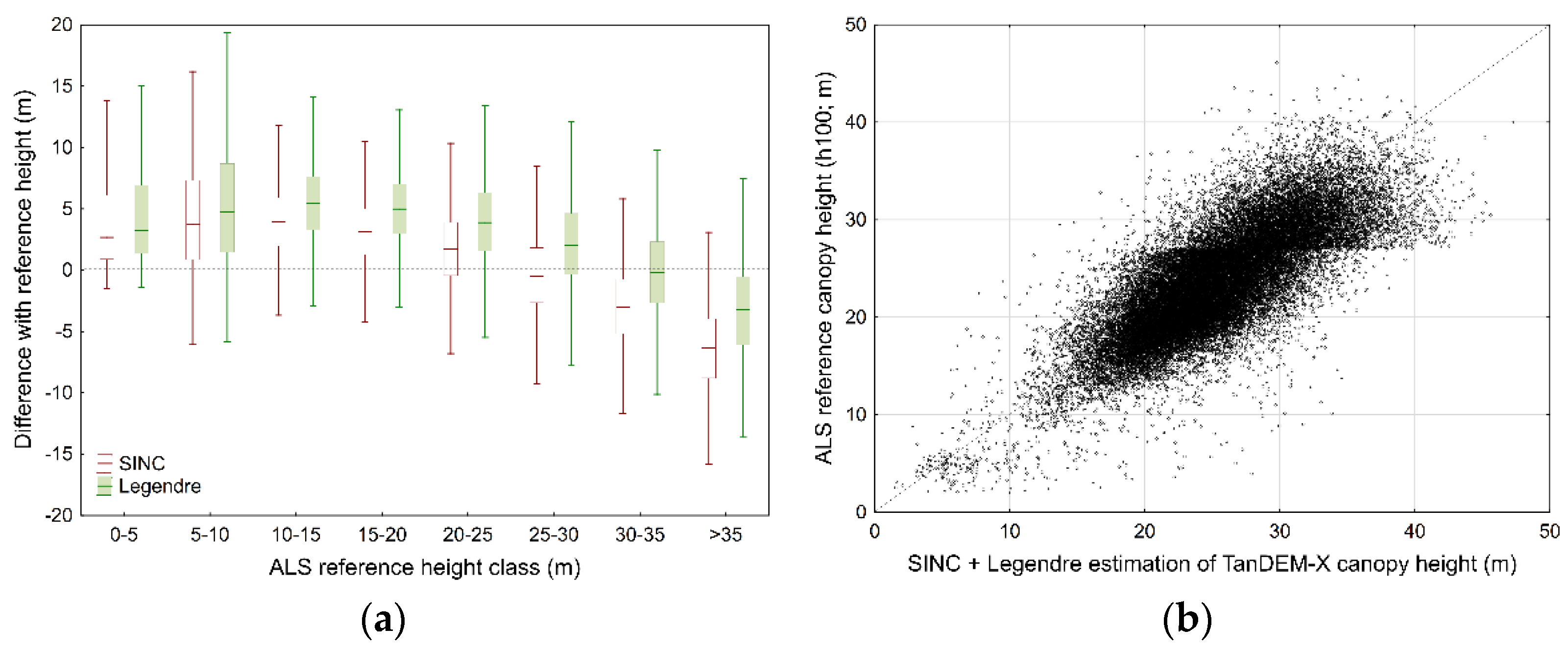
3.3. Validation of TanDEM-X Canopy Height Estimates

The ALS reference data (h100) were used to assess the derived TanDEM-X canopy height estimates. The reference canopy height estimates were subtracted from the derived SINC and Legendre estimates. Validation measures included Pearson correlation (r), and absolute and relative mean difference (MD) and root mean square error (RMSE). Relative MD and RMSE were calculated using the mean of the observed values (h100). Validation was done at the pixel level (i.e., wall-to-wall), excluding pixels where h100 was < 2 m. A Landsat-based forest change product [25] was used to also exclude from the validation any pixels that were disturbed between the time of the TanDEM-X acquisition in 2011 and the ALS acquisition in 2012, and between 2011 and the 2018 forest inventory.

4. Results

We applied the SINC function (0th order of the Legendre series) to generate a wall-to-wall map of canopy height from the 2011 Tandem-X CoSSC data at a 25 m spatial resolution and compared these to the reference ALS wall-to-wall height estimate (h100). When compared to the LiDAR h100, the SINC heights had an r value of 0.71, an MD of 0.89 m (3.77%) and an RMSE of 4.1 m (17.5%; Figure 4a).

Next, we produced a canopy height estimate from the TanDEM-X data using the 6th order Legendre approximation, where a mean GEDI vertical profile was determined for the two-layer forest structure because more than 85% of forest stands in the PRF are classified as having either two-layer (TO) or complex (CX) forest structures and the coherence/height curves for these two profiles are very similar. The Legendre height estimates had an r value of 0.71, an MD of 3.2 m (13.5%) and an RMSE of 5.2 m (22.25%; Figure 4b).

Figure 5a indicates the distribution of differences between the SINC and Legendre canopy height estimates and the reference h100, by 5 metre height class. The SINC approach generally overestimates canopy height until 25–30 m, beyond which SINC underestimates canopy height, with underestimation increasing with increasing canopy height. On the other hand, the Legendre approach had larger overestimation errors than the SINC in the lower canopy height classes and less underestimation in higher canopy height classes (i.e., >25–30 m).

We combined the SINC and Legendre approaches, using the SINC estimate for canopy heights < 27 m (i.e., mid-point of 25–30 m class), and the Legendre estimate where canopy heights ≥ 27 m (Figure 6). The resulting TanDEM-X canopy height estimate had improved agreement with the reference h100 (r = 0.78, MD = 1.68 m (7.16%), RMSE = 1.29 m (5.49%; Figure 5b)). The combined output markedly reduced SINC underestimation for areas of taller trees, whilst avoiding the Legendre overestimations in the areas of lower h_v to hoa ratios (i.e., relatively shorter trees).

5. Discussion

The SINC model provides a robust approach to canopy height estimation from TanDEM-X that has been applied across a range of forest environments [6,7,23,24]; however SINC is known to result in an underestimation of canopy heights in taller forests, a shortcoming that can have implications for estimation of forest biomass. Herein we present a solution to this challenge, which leverages samples of GEDI waveforms in a Legendre series to improve wall-to-wall canopy height estimation. The advantage of the Legendre approach is that it allows us to identify the key spatial frequencies required in a vertical profile to enable an accurate radar height estimation. This knowledge can then be used to inform on profile resolution requirements for supporting LiDAR and radar tomography in future missions. The Legendre series also helps identify those features of the forest canopy that are important for physical interpretation of the radar signal, such as number, location, and width of sub-canopy layers for example. Employing the SINC approach in lower canopy height areas, ensures we avoid overestimation of height in these shorter stature forests (which could also lead to a corresponding overestimation of biomass).

Herein we have demonstrated a novel approach for improving TanDEM-X canopy height estimation using samples of GEDI LiDAR waveforms. However, an important consideration is how to systematically identify areas where SINC underestimates canopy height without support of airborne LiDAR data and/or in situ forest inventory data. Further research is required to determine useful forest structure stratifications that can be derived from spaceborne radar or optical remotely sensed data, which would allow for the automated detection of areas where SINC is underestimating height, wherein appropriate GEDI vertical profiles can be applied in the Legendre approximation described herein.

In our demonstration of the method, we have used either the 0th order (SINC) or the full 6th order Legendre approximation (with three peaks and two nulls) to address either small baseline products (shorter stature trees) or large baseline products (taller stature trees), respectively. An outstanding question is then, how many orders are actually required for the Legendre approximation so that it sufficiently represents the vertical frequency details of a LiDAR vertical profile?

To address this question, we provide an example using profiles for single-layer (SI) forest stands, which represent less than 10% of the forest stands in the PRF. Figure 7a shows the 6th order Legendre approximation (red dash) overlaid on top of the mean SI GEDI profile (black) and the corresponding Legendre spectral amplitude. Figure 7b shows the SINC, 2nd, 4th, and 6th order Legendre approximation. Similar to the two-layer (TO) stands in Figure 3, the SINC reference (green) provides a lower bound on canopy height estimates for any given coherence. The other curves diverged from the SINC with increasing hv/hoa ratio. The Legendre approximation varies with different profiles, such as SI and TO, but whatever its spectrum, the Legendre will provide an increased height estimate for a given coherence, relative to the SINC. For a best-fit profile, the 6th order Legendre approximation (red dash) in both cases apparently sits very well on top of the black curve from the full resolution of a vertical profile. However, the 4th order (cyan dash) also converges well on the black curve for both the SI (Figure 7b) and TO profiles (Figure 3), indicating that the 4th order Legendre approximation may be sufficient for Legendre canopy height estimation in some forest environments; however further investigation is required. The examples shown in Figure 3 and Figure 7b can aid in finalizing how many orders of Legendre approximation are needed and thereby set the spatial frequency requirements for useful profile estimation.

6. Conclusions

In this study, we developed and assessed a novel combined SINC + Legendre approach for fusing high-resolution but sparsely spatially sampled GEDI LiDAR waveforms with TanDEM-X single pass radar interferometry to improve radar wall-to-wall forest canopy height estimation. Herein we used GEDI waveforms simulated at actual GEDI footprints in order to ensure temporal concordance with our TanDEM-X data; however the approach is equally applicable to observed GEDI data. We first generalized our standard SINC forest height estimation algorithm to arbitrary vertical profile by using a Fourier-Legendre approach and then showed that the SINC approach provided a lower bound on canopy height estimates for any given interferometric coherence. Our results indicated that, for small baseline products, the uniform SINC model provided more accurate height estimates and the structure-free assumption is valid. On the other hand, the Legendre method with GEDI LiDAR waveforms was required for large baseline and height products, e.g., greater than 25–30 m in the PRF, where SINC underestimations normally occur. A combined TanDEM-X canopy height estimate from the SINC + Legendre approach had greater correspondence with the reference ALS data and a lower RMSE compared to estimates generated from the SINC or Legendre exclusively. Future research should focus on developing automated forest structure stratifications using spaceborne radar, LiDAR, or optical data to aid in systematically identifying those forest structures where SINC underestimation is more likely to occur. In these areas, the SINC + Legendre approach can be used for optimized forest canopy height mapping over large areas.

References

1. Guliaev, R.; Cazcarra-Bes, V.; Pardini, M.; Papathanassiou, K. Forest Height Estimation by Means of TanDEM-X InSAR and Waveform Lidar Data. IEEE J. Sel. Top. Appl. Earth Obs. Remote Sens. 2021, 14, 3084–3094. [Google Scholar] [CrossRef]
2. Qi, W.; Lee, S.-K.; Hancock, S.; Luttcke, S. Improved forest height estimation by fusion of simulated GEDI Lidar data and TanDEM-X InSAR data. Remote Sens. Environ. 2019, 221, 621–634. [Google Scholar] [CrossRef] [Green Version]
3. Zhao, L.; Chen, E.; Li, Z.; Zhang, W.; Fan, Y. A New Approach for Forest Height Inversion Using X-Band Single-Pass InSAR Coherence Data. IEEE Trans. Geosci. Remote Sens. 2021, 1–18. [Google Scholar] [CrossRef]
4. Cazcarra-Bes, V.; Albrecht, L.; Guliaev, R.; Choi, C.; Pardini, M.; Papathanassiou, K. Mapping global forest canopy height through integration of GEDI and Landsat data. In Proceedings of the Polinsar 2021, Online Event. 30 April 2021. Available online: https://next.brella.io/events/P2021oe/home (accessed on 30 November 2020).
5. Pardini, M.; Cazcarra-Bes, V.; Papathanassiou, K. Forest Height and Structure Estimation by Means of InSAR Data—Using P-band profiles to estimate forest height. In Proceedings of the Polinsar 2021, Online Event. 29 April 2021. Available online: https://next.brella.io/events/P2021oe/home (accessed on 30 November 2020).
6. Chen, H.; Cloude, S.R.; Goodenough, D.G. Forest Canopy Height Estimation Using Tandem-X Coherence Data. IEEE J. Sel. Top. Appl. Earth Obs. Remote Sens. 2016, 9, 3177–3188. [Google Scholar] [CrossRef]
7. Chen, H.; Cloude, S.R.; Goodenough, D.G.; Hill, D.A.; Nesdoly, A. Radar forest height estimation in mountainous terrain using tandem-X coherence data. IEEE J. Sel. Top. Appl. Earth Obs. Remote Sens. 2018, 11, 3443–3452. [Google Scholar] [CrossRef]
8. Cloude, S.R. Polarisation: Applications in Remote Sensing, 2nd ed.; Oxford University Press: Oxford, UK, 2009; ISBN 13: 978-0-19-956973-1. [Google Scholar] [CrossRef]
9. Cloude, S.R. Polarization Coherence Tomography. Radio Sci. 2006, 41, RS4017. [Google Scholar] [CrossRef]
10. Cloude, S.R. Dual Baseline Coherence Tomography. IEEE Geosci. Remote Sens. Lett. 2007, 4, 127–131. [Google Scholar] [CrossRef]
11. Cloude, S.R.; Brolly, M.; Woodhouse, I. A study of forest vertical structure estimation using coherence tomography coupled to a macro-ecological scattering model. In Proceedings of the IEEE International Symposium on Geoscience and Remote Sensing 2009, Cape Town, South Africa, 12–17 July 2009. [Google Scholar] [CrossRef]
12. White, J.C.; Chen, H.; Woods, M.E.; Low, B.; Nasonova, S. The Petawawa Research Forest: Establishment of a Remote Sensing Supersite. For. Chron. 2019, 95, 149–156. [Google Scholar] [CrossRef] [Green Version]
13. Leckie, D.G. Advances in remote sensing technologies for forest surveys and management. Can. J. For. Res. 1990, 20, 464–483. [Google Scholar] [CrossRef]
14. White, J.C.; Penner, M.; Woods, M. Assessing single photon LiDAR for operational implementation of an enhanced forest inventory in diverse mixedwood forests. For. Chron. 2021, 97, 78–96. [Google Scholar] [CrossRef]
15. Kugler, F.; Schulze, D.; Hajnsek, I.; Pretzsch, H.; Papathanassiou, K. TanDEM-X Pol-InSAR Performance for Forest Height Estimation. IEEE Trans. Geosci. Remote Sens. 2019, 52, 6404–6422. [Google Scholar] [CrossRef]
16. Dubayah, R.; Luthcke, S.; Blair, J.; Hofton, M.; Armston, J.; Tang, H. GEDI L1B Geolocated Waveform Data Global Footprint Level V001 [Data Set]; NASA EOSDIS Land Processes DAAC: Washington, DC, USA, 2020. [Google Scholar] [CrossRef]
17. Krehbiel, C. Getting Started with GEDI L1B Version 2 Data in Python. Available online: https://lpdaac.usgs.gov/resources/e-learning/getting-started-gedi-l1b-version-2-data-python/ (accessed on 21 December 2020).
18. Hancock, S.; Armston, J.; Hofton, M.; Sun, X.; Tang, H.; Duncanson, L.; Kellner, J.; Dubayah, R. The GEDI simulator: A large-footprint waveform lidar simulator for calibration and validation of spaceborne missions. Earth Space Sci. 2019, 6, 294–310. [Google Scholar] [CrossRef] [PubMed]
19. Ontario Ministry of Natural Resources and Forestry. Forest Resources Inventory Technical Specifications. 2009. Available online: https://docs.ontario.ca/documents/2837/fim-tech-spec-forest-resources-inventory.pdf (accessed on 30 November 2020).
20. Treuhaft, R.N.; Madsen, S.; Moghaddam, M.; van Zyl, J.J. Vegetation characteristics and underlying topography from interferometric data. Radio Sci. 1996, 31, 1449–1485. [Google Scholar] [CrossRef]
21. Papathanassiou, K.P.; Cloude, S.R. Single baseline polarimetric SAR interferometry. IEEE Trans. Geosci. Remote Sens. 2001, 39, 2352–2363. [Google Scholar] [CrossRef] [Green Version]
22. Cloude, S.R.; Papathanassiou, K.P. Three-stage inversion process for polarimetric SAR interferometry. IEE Proc. Radar Sonar Navig. 2003, 150, 125–134. [Google Scholar] [CrossRef] [Green Version]
23. Chen, H.; Beaudoin, A.; Hill, D.A.; Cloude, S.R.; Skakun, R.S.; Marchand, M. Mapping Forest Height from TanDEM-X Interferometric Coherence Data in Northwest Territories. Canada. Can. J. Remote Sens. 2019, 45, 290–307. [Google Scholar] [CrossRef]
24. Chen, H.; Hill, D.A.; White, J.C.; Cloude, S.R. Evaluating the Impacts of Using Different Digital Surface Models to Estimate Forest Height with TanDEM-X Interferometric Coherence Data. J. Radars 2020, 9, 386–398. [Google Scholar] [CrossRef]
25. Hermosilla, T.; Wulder, M.A.; White, J.C.; Coops, N.C.; Hobart, G.W.; Campbell, L.B. Mass data processing of time series Landsat imagery: Pixels to data products for forest monitoring. Int. J. Digit. Earth 2016, 9, 1035–1054. [Google Scholar] [CrossRef] [Green Version]
Figure 1. 2013 RGB Vexcel UltraCam image of the Petawawa Research Forest captured on 5 September 2013 (a) and an estimate of canopy cover derived from airborne LiDAR data (as percentage of LiDAR returns > 2 m) acquired in August 2012 (b).
Remotesensing 13 02882 g001
Figure 2. Normalized vertical profile stack (a), the mean profile for the TO complexity class (b), mean TO profile (black) and Legendre approximations (red dash) (c) and the corresponding 6th order Legendre spectra (d).
Remotesensing 13 02882 g002
Figure 3. TanDEM-X coherence versus the hv/hoa ratio for five profiles: the reference SINC profile (green), the coherence obtained from full resolution of the two-layer forest (TO) profile (black), the 2nd order (blue dash), the 4th order (cyan dash), and the 6th order Legendre approximation (red dash).
Remotesensing 13 02882 g003
Figure 4. SINC (a) and Legendre (b) TanDEM-x canopy height estimates plotted against ALS h100 reference estimates.
Remotesensing 13 02882 g004
Figure 5. Distribution of differences between the SINC and Legendre TanDEM-X canopy height estimates and the reference ALS-derived h100 canopy height estimates, by 5-metre height classes. Boxplots indicate the median, 25th–75th percentiles, and non-outlier range. (a) SINC + Legendre canopy height estimates plotted against ALS h100 reference estimates (b).
Remotesensing 13 02882 g005
Figure 6. TanDEM-X canopy height estimate over the PRF using the combined SINC + Legendre approach.
Remotesensing 13 02882 g006
Figure 7. 6th order Legendre approximation (red dash) on top of mean SI profile (black) with corresponding Legendre spectra (a) and TanDEM-X coherence versus the hv/hoa ratio for SI profiles: the reference SINC (green), the full profile (black), the 2nd, 4th and 6th order Legendre approximation (blue, cyan and red dash, respectively) (b).
Remotesensing 13 02882 g007
Publisher’s Note: MDPI stays neutral with regard to jurisdictional claims in published maps and institutional affiliations.