Abstract
A good understanding of the accuracy of the Global Positioning System (GPS) surface displacements provided by different processing centers plays an important role in load deformation analysis. We estimate the noise level in both vertical and horizontal directions for four representative GPS time series products, and compare GPS results with load deformation derived from the Gravity Recovery and Climate Experiment (GRACE) gravity measurements and climate models in Europe. For the extracted linear trend signals, the differences among different GPS series are small in all the three (east, north, and up) directions, while for the annual signals the differences are large. The mean standard deviations of annual amplitudes retrieved from the four GPS series are 3.54 mm in the vertical component (69% of the signal itself) and ~ 0.3 mm in the horizontal component (30% of the signal itself). The Scripps Orbit and Permanent Array Center (SOPAC) and MEaSUREs series have the lowest noise level in vertical and horizontal directions, respectively. Through consistency/discrepancy analysis among GPS, GRACE, and model vertical series, we find that the Jet Propulsion Laboratory (JPL) and Nevada Geodetic Laboratory (NGL) series show good consistency, the SOPAC series show good agreements in annual signal with the GRACE and model, and the MEaSUREs series show substantially large annual amplitude. We discuss the possible reasons for the notable differences among GPS time series products.
1. Introduction
Surface load deformations are caused by mass redistributions in the geophysical fluids system, including the atmosphere, ocean, terrestrial water, ice sheets and glaciers, etc. With gradually increasing precision of the Global Positioning System (GPS), one of the most representative Global Navigation Satellite System (GNSS), surface deformation can be fairly accurately observed. In early studies, GPS measurements were combined with data from other geodetic techniques (e.g., satellite gravimetry, altimetry) to study large scale surface loads, such as global water cycling, and polar ice melting [1,2]. With dense and continuous observation sites, GPS can be used as an effective constraint or even an independent means to quantify the magnitude and spatial distribution of surface load [3,4]. A recent study by Knappe et al. [5] showed that GPS observations can be downscaled to reflect local load changes at scales of several tens of kilometers.
For load deformation studies, most researchers prefer directly using the surface displacement time series provided by GPS data centers rather than processing GPS observation data (e.g., pseudo-ranges or -phases). In previous studies, Fu and Freymueller [6] used observations from GPS stations installed by Caltech and other organizations to analyze load deformation in Nepal Himalaya, and Wahr et al. [3] used GPS three-dimensional daily time series provided by the Plate Boundary Observatory Analysis Centers (PBOACs) to study horizontal deformation in California. Besides these products from regional GPS station networks, some global network GPS post-processing time series products using different sorts of software are also used in load deformation studies, such as the Jet Propulsion Laboratory’s (JPL’s) GNSS-Inferred Positioning System (GIPSY) solutions, the Scripps Orbit and Permanent Array Center’s (SOPAC’s) GAMIT solutions, the MEaSUREs combination solutions using the JPL analyze_tserist_filter software package [7,8,9,10], etc. Recently, some new GPS time series products are also available, such as the Nevada Geodetic Laboratory (NGL) GPS series used in Han [11], the Crustal Movement Observation Network of China (CMONOC) used in Wang et al. [12], and the EUREF Permanent Network (EPN) used in Springer et al. [13], etc.
The magnitude of surface load deformation is at the millimeter level for both seasonal and long-term signals in the vertical direction, and even smaller in the horizontal direction, and the ratio of the vertical to the horizontal is ~ 2.0 to 3.0 [3,14]. The discrepancies among the currently available GPS time series products reach as large as several millimeters at some stations, which are at the same level as the load deformation signal, and are expected to affect load deformation analyses [15,16]. Gu et al. [17] quantified the vertical load deformations from multi-institution GPS solutions at some selected global sites, and found that the post-processing error of GPS data is the main reason for the differences among different time series products. However, for horizontal and regional GPS surface displacements, which also provide important mass load constraint especially for regional or local load study, the differences and their corresponding impact on load analysis need further study.
Besides, Kenyeres et al. [18] integrated the GNSS positions and velocities of the EPN stations and analyzed the quality of their homogenization. They focused on the evaluation of data processing approaches, such as mathematical testing and assessment of the alignment with the International Terrestrial Reference Frame (ITRF) position, rather than analysis of the contained geophysical signals in the time series. Martens et al. [19] applied a total root mean square (RMS) scatter to the five GPS series and discussed their overall quality in the contiguous USA and Alaska, and further explored the impacts of the different atmospheric models.
In this study, we chose four representative public GPS time series products, and carried out a comprehensive evaluation of the consistency/discrepancy among these solutions for both the vertical and horizontal components of surface displacements in the Europe region. The GPS results were compared with load deformations derived from the Gravity Recovery and Climate Experiment (GRACE) satellite gravity measurements and surface mass loads predicted by advanced atmospheric, oceanic, and hydrological models. Relative accuracies of the six load deformation results (four GPS series, GRACE, and models) were assessed using the Three-Cornered Hat (TCH) method. In-depth assessment of GPS measurement accuracy is important for understanding and interpreting load deformation and reconciling different GPS processing strategies.
2. Materials and Methods
2.1. GPS Time Series Products
We use the four three-dimensional daily GPS time series from JPL, SOPAC, MEaSUREs combination [20], and NGL [21]. As suggested by the International Global Navigation Satellite Systems Service (IGS), the nontidal load signals (from the atmosphere, ocean, and surface hydrology) are fully retained in these products, while the tidal effects are removed. To be comparable with GRACE time series, we select the GPS time series over the period January 2007 to June 2017, which cover the GRACE mission period and has a time span of 10 years. This data length is adequate to retrieve the annual signals as well as the linear trend in recent years.
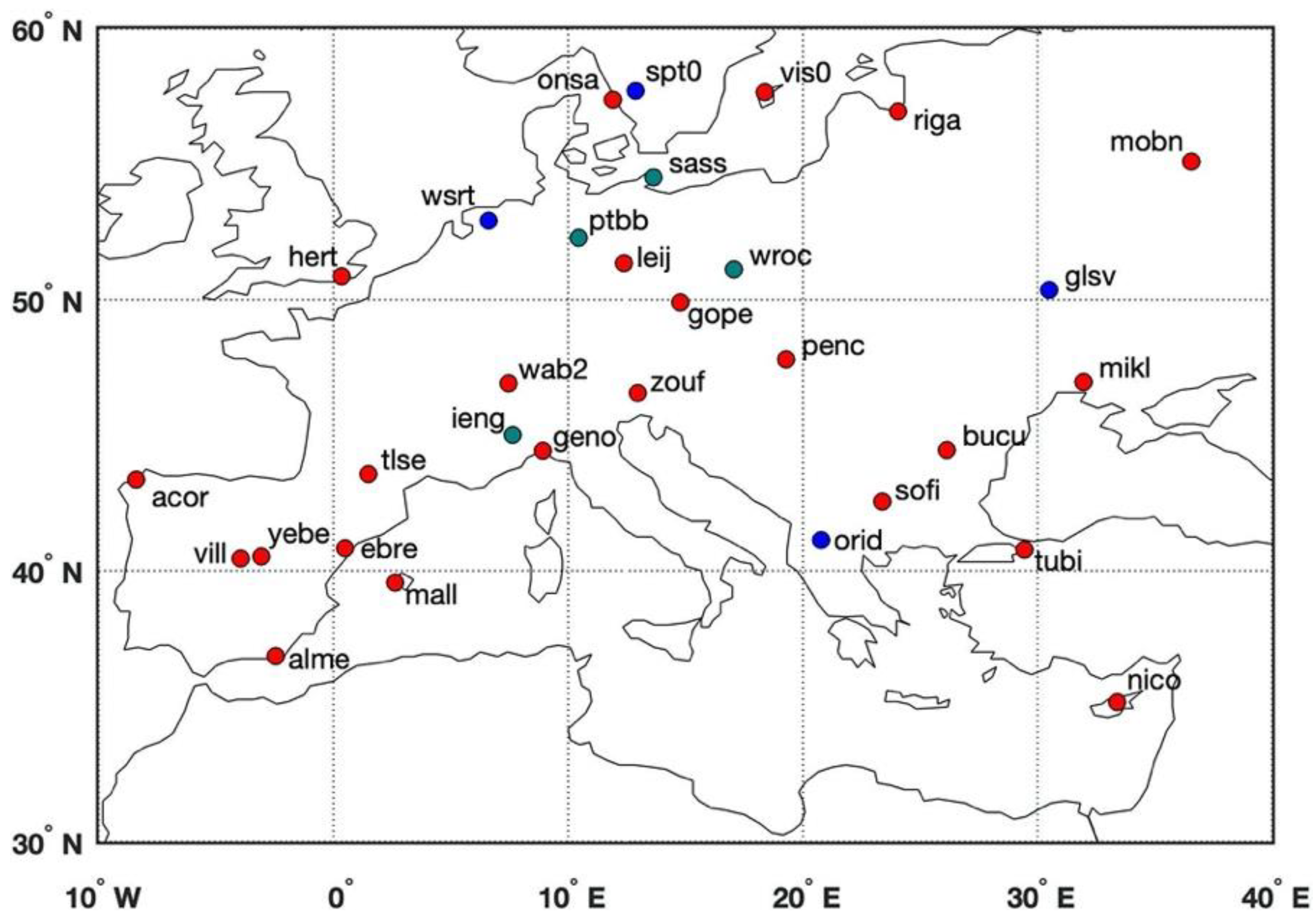
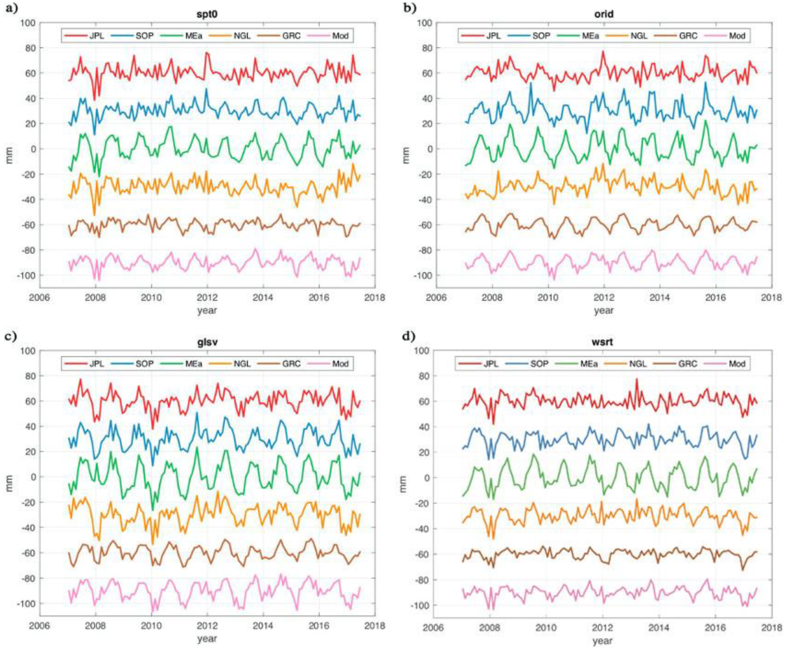
We select 31 sites in the Europe region based on the data quality (with data gaps no longer than 1 month, and without obvious “jumps” due to receiver changing or tectonic motions). Compared with the sites used in Kenyeres et al. [18], as mentioned above, the number of the selected sites in this study is far less than theirs (several hundred) due to the limited number of sites to guarantee continuous data availability of the four selected GPS post-processing time series products. Despite the relatively smaller number of selected sites, the variety of GPS data processing software (described in the websites of products) and the generally uniform spatial distribution of our site selection well satisfy the uncertainty study of load deformation. Figure 1 shows the locations of the 31 GPS sites in Europe. The daily GPS height time series at four selected sites (marked with blue dots in Figure 1) are shown in Figure 2, displaying the surface height changes from the four products, with artificial offsets added (to each series) for clarity. Substantially large discrepancies among the four GPS series clearly exist, especially at seasonal time scales. The comparison for the other sites is provided in Figures S1 and S2 for conciseness.

Figure 1.
Locations of the selected 31 GPS sites in Europe. The blue dots denote the sites whose vertical displacements are shown in Figure 2, while the green dots denote the sites whose horizontal displacements are shown in Figure 6. Note that the time series at the site glsv are shown in both vertical and horizontal directions (in Figure 2 and Figure 6).
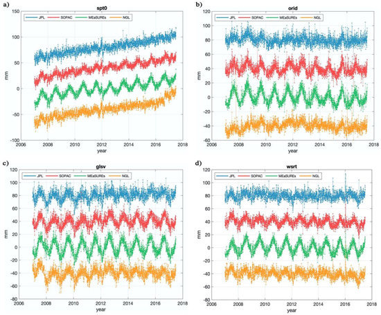
Figure 2.
Vertical displacements at (a) spt0, (b) orid, (c) glsv, (d) wsrt (marked with blue dots in Figure 1) from the four GPS time series products. Vertical offsets are added for clarity.
In order to be comparable with the GRACE and model data (described later), the GPS daily series are averaged and re-adjusted to align at monthly temporal resolution through the following steps. We first fill the gaps using the method based on Singular Spectrum Analysis (SSA) introduced by Kondrashov et al. [22], and then apply a 31-day moving average filter and interpolate into monthly intervals afterwards.
2.2. GRACE Load Deformation
We use the GRACE Release 6 (RL06) mascon solutions from January 2007 to June 2017, provided by the Center for Space Research (CSR) at the University of Texas at Austin (http://www2.csr.utexas.edu/grace/RL06_mascons.html, accessed on 18 June 2020) [23]. In the CSR RL06 mascon solutions (named as “CSR GRACE/GRACE-FO RL06 v02 Mascon Grids w/ Corrections Applied”), the C20 and C30 coefficients are replaced by Satellite Laser Ranging estimates [24], and degree-1 coefficients (C11, S11, C10) are included using the geocenter series provided in the GRACE supplementary datasets (in GRACE Technical Note 13) [25,26]. The Glacial Isostatic Adjustment (GIA) effects have been removed using the ICE-6G_D (VM5a) model [27], and the GRACE GAD fields have been restored (so over the ocean, the mascon mass change represents ocean bottom pressure change). We remove the GAD contributions and add back the GAC contributions to make the GRACE results comparable with the GPS solutions (both including atmospheric, oceanic, and hydrological load effects).
To estimate the vertical displacements using GRACE mascon products, we first convert the gridded mass distribution to fully normalized spherical harmonic (SH) Stokes coefficients up to degree and order 360, and then calculate the vertical load displacements at a given point (with the colatitude and longitude ) using the following Equations (1)–(3) [28,29].
where and are the dimensionless SH coefficients defined in Equation (9) of Wahr et al. [29], is the mean radius of the Earth, are the normalized Legendre functions of degree and order , is the area element (namely, ), is the density of water, is the average density of the Earth, and and are the elastic load Love numbers of degree for the Preliminary reference Earth model (PREM) [30] given by Han and Wahr [31]. The GRACE series are also re-aligned into monthly intervals using the same method as applied to the GPS series (described in Section 2.1).
2.3. Climate Models
The total load is estimated by the sum of atmospheric, oceanic, and hydrological models, which are monthly mass changes of the non-tidal atmosphere and ocean from the Atmosphere and Ocean Level-1B (AOD1B) De-Aliasing GAC products in degree 180 Stokes coefficients [32], and monthly terrestrial water storage (TWS) changes from the Global Land Data Assimilation System (GLDAS) Noah land surface model (V2.1) [33]. Consistent with the processing steps for GRACE data in Section 2.2, the mass distributions from climate models are converted to the load displacements using Equations (1)–(3). Noteworthily, in order to consider the global mass conservation, we set the degree 0 of GAC Stokes coefficients (representing the global total mass change of the atmosphere and ocean) to zero, and add to the ocean the negative mean value of the total GLDAS mass change over continent (assuming the total mass change of TWS is from the ocean).
3. Results
3.1. Uncertainty Assessment of GPS Height Solutions
The annual components (amplitudes and phases) and linear trends of the four GPS height time series products at the 31 selected sites are obtained using least squares fitting are listed in Table 1. The linear trend signals at most sites are small (less than 1 mm/year), except for those in Scandinavia Peninsula with strong uplift rates (apparently due to the GIA effect over this region). To quantify the dispersion of the statistical values from the four products, we estimate the mean values and standard deviations (SD) of the annual amplitudes, annual phases, and linear trends at the GPS sites, and the results are shown in Table 2. Note that for sites with large differences among the four products, the mean values of annual amplitudes and phases can hardly reflect the real deformation signals, and are only calculated as a value for joint analysis combined with the SD.

Table 1.
Annual amplitudes (ann. amp.), annual phases (ann. pha.) and trends of the four height time series products at the 31 GPS sites.

Table 2.
Mean values and standard deviations of the four statistical values in Table 1 at each site.
The mean SD of the annual amplitude is 3.54 mm, which is at the same level as that of the load signal (with an average value of 5.15 mm), while the mean SD of the annual phase is 23.9 degree, equal to ~1 month in the annual cycle. Since the weak linear trend signal (with an average value of ~0.05 mm/year) may be under the precision of the GPS observations, it would be difficult to use the mean SD (0.29 mm/year) to quantify the dispersion among multi-institution GPS products. Apparently, the large differences of GPS height displacements are expected to hinder the correct interpretation of load deformation, especially for the annual signals.
Considering the much smaller magnitudes of the trends in the studied region, and that the differences are mostly at seasonal time scales, we detrend all the time series and apply the “Three-Cornered Hat” method [34] to further assess the accuracy for each GPS series. To be consistent with subsequent experiments with the GRACE and model data, the GPS series are monthly averaged. With the assumption that the noises of the GPS products are independent from each other, it is possible to compute the SD of noise residuals in each series using least squares estimation. For a common signal (e.g., surface deformation), each observation can be expressed as a sum of true signal plus noise in Equation (4) as follows.
Computing the variance of the difference between any two of the time series by eliminating the common terms, we obtain the 6 equations with 4 variances to be determined, as shown in Equation (5).
The least squares solutions of Equation (5) are the noise variances, and the estimated SDs (square roots of variances) are shown in Table 3. The SOPAC height time series show the lowest noise level at 22 of the 31 sites among the 4 GPS products, while the NGL series yields lowest noise level at 7 sites. The mean SD of noise residuals for the JPL, SOPAC, MEaSUREs, NGL solutions are ~3.70 mm, 2.47 mm, 5.23 mm, and 2.85 mm, respectively.

Table 3.
Standard deviation (SD) of the noise in each site’s height time series, from least squares fit to obtain the variance of difference between each time series pair with the four GPS products (JPL, SOPAC, MEaSUREs, NGL). The lowest SD of noise residuals for each site are highlighted in bold font. (Unit: mm).
3.2. Uncertainty Assessment of Load Deformations from GPS, GRACE, and Models
We also estimate the SD of noise residuals using the TCH method by including load deformations at the 31 sites derived from GRACE and climate model data. Figure 3 shows the comparison among the 6 time series (4 GPS + GRACE + MODEL) at 4 selected sites (same as the sites in Figure 2). The comparison for the other sites is provided in Figures S3 and S4 for conciseness. The four GPS series are monthly averaged, and the GRACE series are resampled into monthly to be comparable with each other. The reasons why we consider the data from the observations by other technique observations are: (a) not all GPS time series products are completely independent from one another, which is the prerequisite of applying the TCH method, (b) GPS observations need independent data from other techniques to validate and interpret, and (c) we also aim to assess the noise level among different techniques.

Figure 3.
Vertical displacements at (a) spt0, (b) orid, (c) glsv, (d) wsrt (marked with blue dots in Figure 1) from the four GPS products, GRACE (GRC) and climate models (Mod). Vertical offsets are added for clarity.
When considering the 6 series, we generate 15 equations with 6 variances to be solved in the form of Equation (5). Table 4 shows the estimated SD of the noise residuals for the time series at each site and the mean values (of the 31 sites) for each technique. The SOPAC height series have the lowest noise standard deviations for 14 of the 31 sites, with the smallest mean value of 2.95 mm. The MEaSUREs shows the largest mean value of 5.42 mm, which is consistent with the conclusion drawn in Table 3 (when using 4 GPS series only).

Table 4.
Standard deviation of the noise in each site’s height time series, from least squares fit to the variance of difference between each time series pair with the six estimates (JPL, SOPAC, MEaSUREs, NGL, GRACE, MODEL). The lowest SD of noise residuals for each site are highlighted in the bold font. (Unit: mm).
Besides assessing the accuracy with noise variance, we implement three additional indicators to assess the consistency/discrepancy among the six series, which are the zero-lag correlation coefficients in Table 5, mean annual amplitude (AnnAmp) reduction in Table 6, and mean root mean squares (RMS) reduction in Table 7. The correlation coefficient reflects the closeness between two variables, which describes the consistency of time variations (phases) between two time series in this study. The annual amplitude reduction is defined as Equation (6), and represents the consistency of annual amplitudes between the two series, while the RMS reduction is defined as Equation (7) and represents the consistency of the total series (including the annual signal as well as other signals/noises).

Table 5.
Mean correlation coefficients among the 6 series.

Table 6.
Mean annual amplitude reductions of the 6 series 1.

Table 7.
Mean RMS reductions of the 6 series 1.
The largest correlation coefficient is 0.87 (Table 5), which implies a good consistency of time variations between GRACE and models. Moreover, the corresponding values of mean AnnAmp reduction (73.09 and 66.00, in Table 6) and RMS reduction (49.94 and 30.53, in Table 7) is also large, representing their good consistencies in the studied time scales. In fact, this is in line with expectations since the GRACE series are derived from the mascon and GAC data, while the model series also consist of GAC data and the GAC effect accounts for a large proportion in the time series.
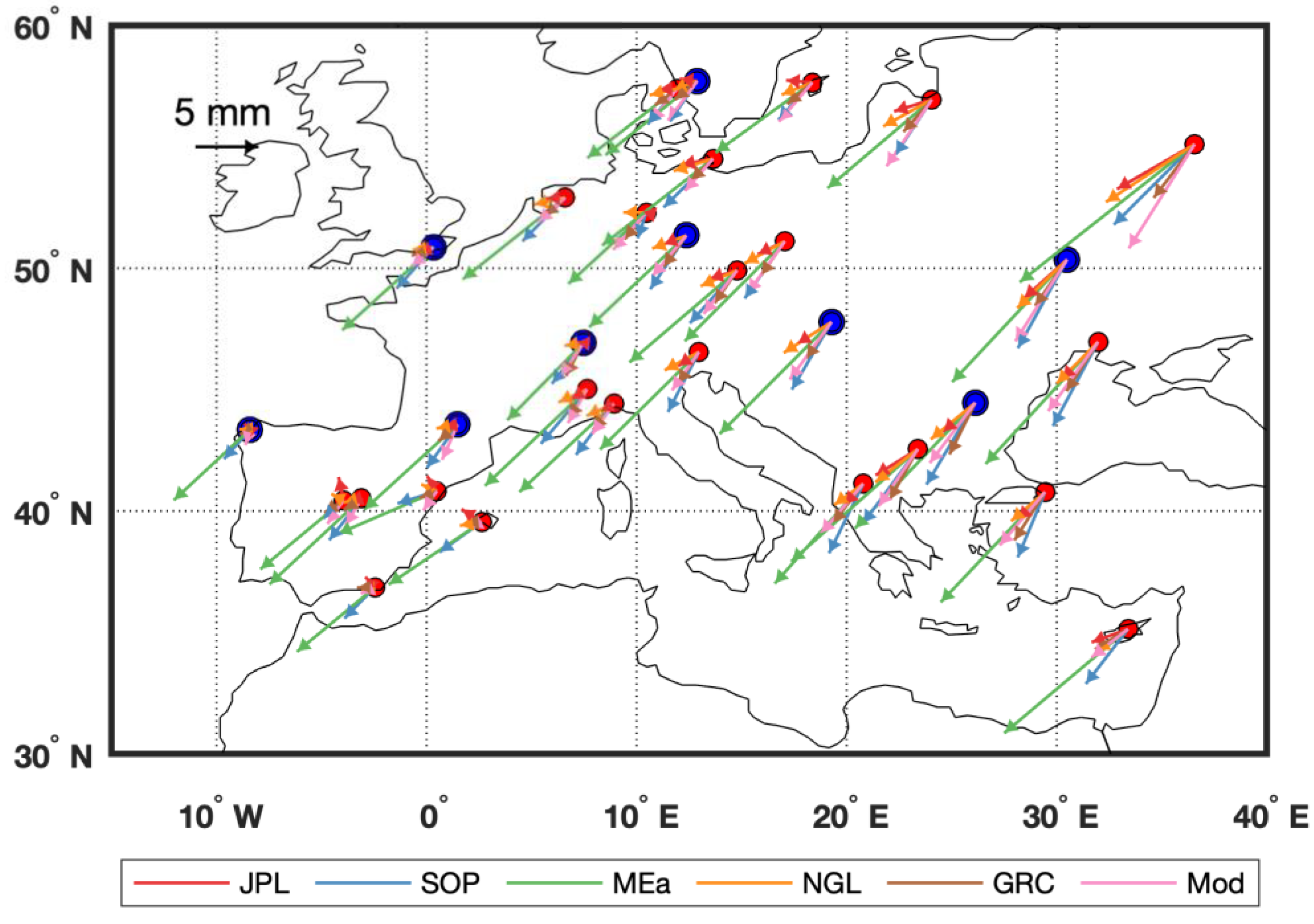
Among the four GPS series, the MEaSUREs series show apparent larger correlation coefficients with the GRACE and model (0.67 and 0.75) than the other three do (see Table 5). The MEaSUREs mean AnnAmp reduction values are all negative (see column 4 in Table 6), representing that the MEaSUREs series have specifically larger annual amplitudes, which can be further illustrated through the phasor diagram (as described subsequently) in the selected sites (see the green vectors in Figure 5). Similarly, the mean RMS reduction values of the MEaSUREs series (see column 4 in Table 7) are smaller than those of the other series, which implies that the MEaSUREs series include stronger fluctuations (or variations) than the others do. Besides, the relatively larger values of the three indicators between JPL and NGL series suggest that there is a good consistency between the two products.
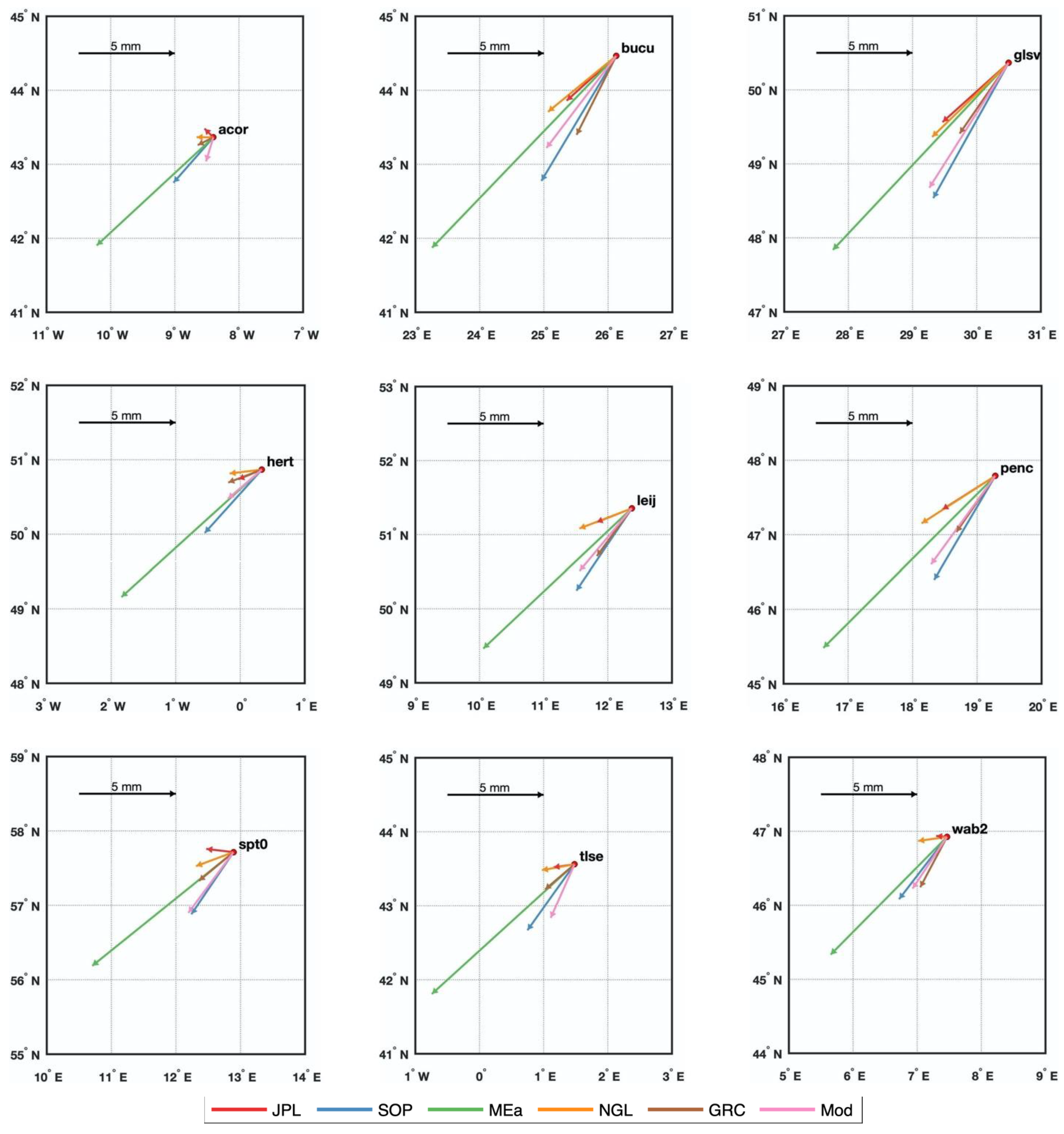
The comparison of the annual signals among the GPS, GRACE and model series using phasor diagrams for all the 31 sites is illustrated in Figure 4. To examine the detailed information of the arrows, we show in Figure 5 the zoomed-in figures of the annual amplitudes and phases at the selected 9 sites, whose annual variations are significant and representative of the study region. The MEaSUREs series exhibit substantially large annual variations, which is consistent with that revealed by Figure 2. In addition, the JPL and NGL series show a consistent pattern of variation, with relatively smaller annual amplitudes and phases, while the SOPAC series show the largest annual phase among the four GPS series at most of the selected sites. Compared with the other three GPS series, the SOPAC annual signals (blue vectors in Figure 5) are closer to the GRACE and model (brown and pink vectors in Figure 5).

Figure 4.
Phasor diagram of annual signal comparisons among GPS, GRACE, and model results at 31 sites. The length of the arrow represents the annual amplitude, and the direction of the arrow denotes the peak-value month counted counterclockwise from the east. The scale of the arrow is marked on the upper left. The blue dots denote the 9 selected sites whose zoomed-in figures are shown in Figure 5.
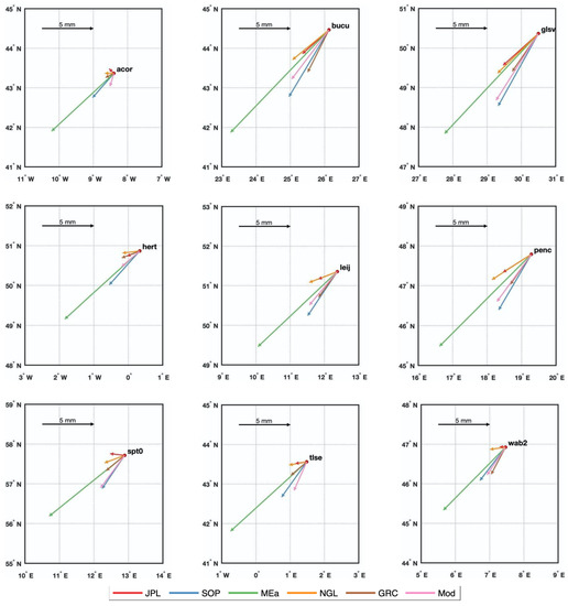
Figure 5.
Phasor diagram of annual signal comparisons among GPS, GRACE and model results at the selected 9 sites. The length of arrow represents the annual amplitude, and the direction of arrow denotes the peak-value month counted counterclockwise from the east. The scale of the arrow is marked on the upper left in each panel.
3.3. Uncertainty Assessment GPS Horizontal Time Series Solutions
In order to further evaluate the GPS load deformations, we analyze the horizontal displacements (east (E) and north (N) directions separately) in Europe using the same method. For the E-direction, Table S1 shows the annual and trend signals for each site using the four GPS time series products, and Table S2 shows the corresponding mean values and standard deviations of the four values. Similarly, Tables S3 and S4 show the same statistical values for the N-direction time series.
For the horizontal linear trend signals, which mainly reflect regional tectonic motions, the magnitudes reach tens of millimeters per year (much larger than that of the U-direction with less than 0.1 mm/year in Table 2), while the SD of the four products (E-direction mean: 0.14 mm/year, N-direction mean: 0.16 mm/y) are at the same level as the U-direction in Table 2 (0.29 mm/year). We assume that the differences in the linear trends estimated from multi-institutional GPS products are small for both vertical and horizontal directions.
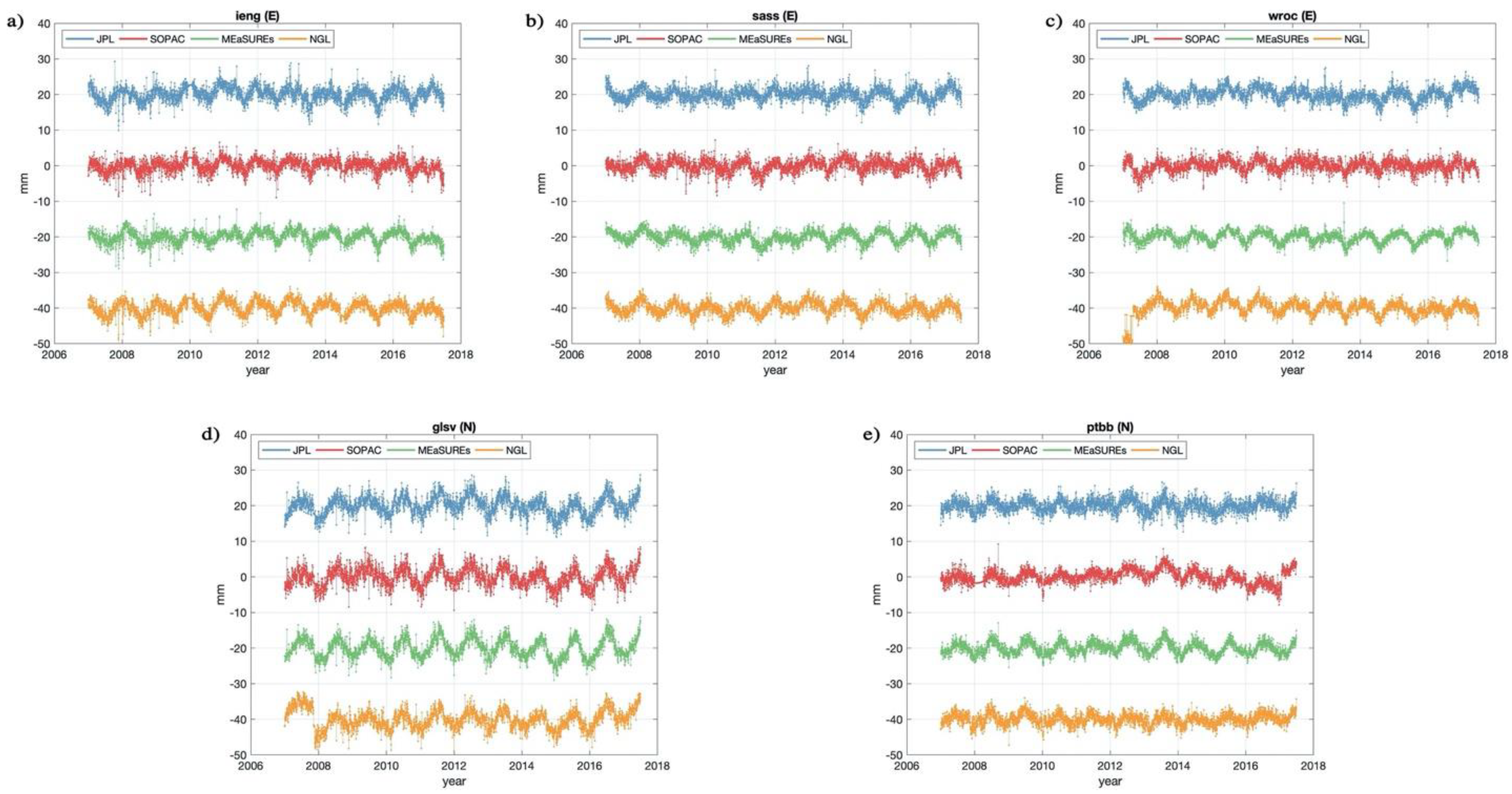
Although GPS horizontal components have been proved to have higher precision than in the vertical direction [35], the load signal in the horizontal direction is only ~30% to 50% of that in the vertical direction [3], which is more difficult to isolate and interpret. Most of the annual amplitudes are less than 1 mm (see Tables S1 and S3), which can hardly reflect the true load signals under the current precision of GPS observation. The only five sites with annual amplitudes larger than 1 mm for all the four GPS series (ieng, sass, wroc for the E direction and glsv, ptbb for the N direction) are selected (marked with green dots in Figure 1), and the SD of their annual amplitudes from the four GPS products are ~0.3 mm, which is about 30% of the observed signal.
We plot the horizontal deformation time series of the five sites in Figure 6, and show residuals of the SD of noise estimated using the TCH method in Table 8. It is interesting to note that for the horizontal components, the MEaSUREs results have the lowest SD of noise for all the five sites, which is contrary to the conclusions in the vertical components.
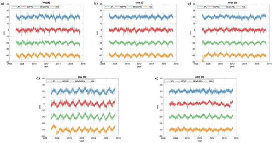
Figure 6.
E-direction displacements at (a) ieng, (b) sass, (c) wroc and N-direction displacements at (d) glsv, (e) ptbb (marked with green dots in Figure 1) with all the four GPS time series products (vertical offsets are added for clarity).

Table 8.
Standard deviation of noise in the five selected sites’ east/north-direction time series, from least squares fit to variance of the difference between each time series pair with the four estimates (JPL, SOPAC, MEaSUREs, NGL). The lowest SD of noise residuals for each site is highlighted in bold font. (Unit: mm).
4. Discussion
The GPS data processing strategy affects the accuracy of generated time series, and may cause bias in load deformation analysis. The JPL and NGL products, which use the Precise Point Positioning (PPP) strategy, show comparable SD of noise residuals (see Table 3 and Table 4) and relatively large values of the three indicators (as shown in Table 5Table 6 and Table 7). The SOPAC series are generated using a distributed sub-network analysis strategy, which pays more attention to regional overall quality and may be more appropriate for regional-scale signal analysis (e.g., load deformation). As for the MEaSUREs, which is a post-processing product based on the JPL and SOPAC data, there may be some artificial variations associated with the processing procedure that is expected to be likely responsible for the large annual amplitudes in Figure 4 and Figure 5.
Compared to vertical deformation analysis, accurate quantification of horizontal deformation is also important for load studies, especially for the inversion of mass load using GPS observations. Our estimates of noise level for the horizontal components show that the MEaSUREs series have the lowest SD of noise. However, the annual amplitudes of horizontal load displacements over most part of Europe are less than 1 mm, which is most likely under the current precision of GPS positioning, and are difficult to be verified by GPS techniques. There could be some levels of dependence among the noises of the four GPS products, which affects the compliance with the assumption of noise independence in the TCH method. In regions with large load signals, more stations are needed so as to provide adequate spatial constraint to determine the location and magnitude of the mass load source. Further analysis is needed in future study.
5. Conclusions
We carried out a detailed comparison of GPS surface displacement time series products from four institutions (namely, JPL, SOPAC, MEaSUREs, and NGL) in Europe, and analyzed their influences on load deformation study. The extracted linear trends of GPS load deformation, whether in the east, north, or vertical direction, showed good agreement among the four products, while the annual variations showed large discrepancies. The mean value of the standard deviations of the four GPS series at 31 sites was ~3.54 mm in annual amplitude of the vertical component (~69% of the signal), and ~0.3 mm for the horizontal component (~30% of the signal). We used the TCH method to estimate the noise level of each series, and found that either four or six time series (four GPS + GRACE + model) were considered, and that the SOPAC vertical series had the lowest SD of noise, revealing its relatively better accuracy. The MEaSUREs time series are likely to include some artificial variations and deviate distinctly in vertical direction from the GRACE-derived and the climate-model-predicted load deformations in Europe. The horizontal displacements are smaller than 1 mm in annual amplitudes for most of the sites in Europe, which are still challenging to be used for load analysis. However, the potential spatial constraint introduced by horizontal displacements deserves continuous attention and further study.
With the development for more than 20 years, the GNSS positioning precision reaches cm or sub-cm level, which is similar to the magnitude of load deformation signals. Due to different data processing strategies (orbit/clock solving strategies, applied correction models, etc.), the discrepancies in the three-dimensional deformation time series are still significant and affect the practical accuracy of GNSS positioning, which cannot be ignored for reliable load deformation analysis, especially for mass load inversion studies using GNSS technique. How to improve the practical accuracy of GNSS load deformation remains a major challenge and is essential to reliable load deformation interpretation as well as quantitative mass variation study of the Earth system.
Supplementary Materials
The following are available online at https://www.mdpi.com/article/10.3390/rs13142765/s1, Figure S1: Vertical displacements for all the other sites (besides the four sites shown in Figure 2) from the four GPS time series products. Vertical offsets are added for clarity. (part 1), Figure S2: Vertical displacements for all the other sites (besides the four sites shown in Figure 2) from the four GPS time series products. Vertical offsets are added for clarity. (part 2), Figure S3: Vertical displacements for all the other sites (besides the four sites shown in Figure 3) from the four GPS products, GRACE (GRC) and climate models (Mod). Vertical offsets are added for clarity. (part 1), Figure S4: Vertical displacements for all the other sites (besides the four sites shown in Figure 3) from the four GPS products, GRACE (GRC) and climate models (Mod). Vertical offsets are added for clarity. (part 2), Table S1: Annual amplitudes (ann. amp.), annual phases (ann. pha.) and trends of the four E-direction time series products at the 31 GPS sites, Table S2: Mean values and standard deviations of the four statistical values in Table S1 at each site, Table S3: Annual amplitudes (ann. amp.), annual phases (ann. pha.) and trends of the four N-direction time series products at the 31 GPS sites, Table S4: Mean values and standard deviations of the four statistical values in Table S3 at each site.
Author Contributions
Conceptualization, S.-Y.W. and J.C.; methodology, S.-Y.W. and J.C.; software, S.-Y.W.; validation, S.-Y.W. and J.L.; writing—original draft preparation, S.-Y.W.; writing—review and editing, S.-Y.W., J.L., J.C. and X.-G.H.; funding acquisition, S.-Y.W., J.L. and X.-G.H. All authors have read and agreed to the published version of the manuscript.
Funding
The research leading to these results received funding from the Natural Science Foundation of Shanghai under Grant Agreement Nos. 19ZR1466900 and 20ZR1467400, and the Natural Science Foundation of China under Grant Agreement Nos. 12003057 and 11873075. The research is supported by the Opening Project of Shanghai Key Laboratory of Space Navigation and Positioning Techniques.
Institutional Review Board Statement
Not applicable.
Informed Consent Statement
Not applicable.
Data Availability Statement
The JPL, SOPAC and MEaSUREs GPS time series datasets analyzed during the current study are available in the GPS Explorer repository, ftp://sopac-ftp.ucsd.edu/pub/timeseries/measures/ats/, accessed on 28 September 2019. The NGL GPS time series datasets analyzed during the current study are available in the Nevada Geodetic Laboratory website, http://geodesy.unr.edu/NGLStationPages/GlobalStationList, accessed on 7 November 2019. The GRACE mascon datasets analyzed during the current study are available in the Center for Space Research website, http://www2.csr.utexas.edu/grace/RL06_mascons.html, accessed on 18 June 2020. The AOD1B GAC datasets analyzed during the current study are available at ftp://rz-vm152.gfz-potsdam.de/grace/Level-2/CSR/RL06/, accessed on 18 June 2020. The GLDAS datasets analyzed during the current study are available in the Goddard Earth Sciences Data and Information Services Center (GES DISC), https://hydro1.gesdisc.eosdis.nasa.gov/opendap/GLDAS/GLDAS_NOAH025_M.2.1/contents.html, accessed on 18 March 2020.
Acknowledgments
We are grateful to the two anonymous reviewers for their insight comments and constructive suggestions. We are grateful to the Assistant Editor, Academic Editor and English Editor for their great help to improve our work. We acknowledge the GPS Explorer archive for providing the JPL, SOPAC, and MEaSUREs time series products, and the Nevada Geodetic Laboratory for providing their publicly available processed GPS data. We acknowledge the Center for Space Research (CSR) for providing the GRACE mascon data, the GeoForschungsZentrum (GFZ) for providing the AOD1B GAC data, and the Goddard Earth Sciences Data and Information Services Center (GES DISC) for providing the GLDAS data. This research was supported by the Natural Science Foundation of China (12003057, 11873075), the Natural Science Foundation of Shanghai (19ZR1466900, 20ZR1467400), and the Opening Project of Shanghai Key Laboratory of Space Navigation and Positioning Techniques. The authors SYW, JL and XGH are grateful to the membership of Laboratory of Astronomy and Space Technology Applications at Shanghai Astronomical Observatory, Chinese Academy of Sciences. This work made use of the High Performance Computing Resource in the Core Facility for Advanced Research Computing at Shanghai Astronomical Observatory, Chinese Academy of Sciences.
Conflicts of Interest
The authors declare no conflict of interest.
References
- Tregoning, P.; Watson, C.; Ramillien, G.; McQueen, H.; Zhang, J. Detecting hydrologic deformation using GRACE and GPS. Geophys. Res. Lett. 2009, 36, L15401. [Google Scholar] [CrossRef] [Green Version]
- Khan, S.A.; Wahr, J.; Stearns, L.A.; Hamilton, G.S.; van Dam, T.; Larson, K.M.; Francis, O. Elastic uplift in southeast Greenland due to rapid ice mass loss. Geophys. Res. Lett. 2007, 34, L21701. [Google Scholar] [CrossRef] [Green Version]
- Wahr, J.; Khan, S.A.; van Dam, T.; Liu, L.; van Angelen, J.H.; van den Broeke, M.R.; Meertens, C.M. The use of GPS horizontals for loading studies, with applications to northern California and southeast Greenland. J. Geophys. Res. Solid Earth 2013, 118, 1795–1806. [Google Scholar] [CrossRef] [Green Version]
- Fu, Y.; Argus, D.F.; Landerer, F.W. GPS as an independent measurement to estimate terrestrial water storage variations in Washington and Oregon. J. Geophys. Res. Solid Earth 2015, 120, 552–566. [Google Scholar] [CrossRef]
- Knappe, E.; Bendick, R.; Martens, H.R.; Argus, D.F.; Gardner, W.P. Downscaling Vertical GPS Observations to Derive Watershed-Scale Hydrologic Loading in the Northern Rockies. Water Resour. Res. 2019, 55, 391–401. [Google Scholar] [CrossRef]
- Fu, Y.; Freymueller, J.T. Seasonal and long-term vertical deformation in the Nepal Himalaya constrained by GPS and GRACE measurements. J. Geophys. Res. Solid Earth 2012, 117, B03407. [Google Scholar] [CrossRef]
- Yan, H.; Chen, W.; Yuan, L. Crustal vertical deformation response to different spatial scales of GRACE and GCMs surface loading. Geophys. J. Int. 2016, 204, 505–516. [Google Scholar] [CrossRef] [Green Version]
- Xu, C. Evaluating mass loading products by comparison to GPS array daily solutions. Geophys. J. Int. 2017, 208, 24–35. [Google Scholar] [CrossRef]
- Argus, D.F.; Landerer, F.W.; Wiese, D.N.; Martens, H.R.; Fu, Y.; Famiglietti, J.S.; Thomas, B.F.; Farr, T.G.; Moore, A.W.; Watkins, M.M. Sustained Water Loss in California’s Mountain Ranges During Severe Drought From 2012 to 2015 Inferred From GPS. J. Geophys. Res. Solid Earth 2017, 122, 10. [Google Scholar] [CrossRef] [Green Version]
- Argus, D.F.; Fu, Y.; Landerer, F.W. Seasonal variation in total water storage in California inferred from GPS observations of vertical land motion. Geophys. Res. Lett. 2014, 41, 1971–1980. [Google Scholar] [CrossRef]
- Han, S.-C. Elastic deformation of the Australian continent induced by seasonal water cycles and the 2010–2011 La Niña determined using GPS and GRACE. Geophys. Res. Lett. 2017, 44, 2763–2772. [Google Scholar] [CrossRef]
- Wang, L.; Chen, C.; Du, J.; Wang, T. Detecting seasonal and long-term vertical displacement in the North China Plain using GRACE and GPS. Hydrol. Earth Syst. Sci. 2017, 21, 2905–2922. [Google Scholar] [CrossRef] [Green Version]
- Springer, A.; Karegar, M.A.; Kusche, J.; Keune, J.; Kurtz, W.; Kollet, S. Evidence of daily hydrological loading in GPS time series over Europe. J. Geod. 2019, 93, 2145–2153. [Google Scholar] [CrossRef]
- Pinel, V.; Sigmundsson, F.; Sturkell, E.; Geirsson, H.; Einarsson, P.; Gudmundsson, M.T.; Högnadóttir, T. Discriminating volcano deformation due to magma movements and variable surface loads: Application to Katla subglacial volcano, Iceland. Geophys. J. Int. 2007, 169, 325–338. [Google Scholar] [CrossRef] [Green Version]
- Wang, S.Y.; Chen, J.L.; Wilson, C.R.; Li, J.; Hu, X. Reconciling GRACE and GPS estimates of long-term load deformation in southern Greenland. Geophys. J. Int. 2018, 212, 1302–1313. [Google Scholar] [CrossRef]
- Wang, S.Y.; Chen, J.L.; Wilson, C.R.; Li, J.; Xiao-Gong, H. Vertical motion at TEHN (Iran) from Caspian Sea and other environmental loads. J. Geodyn. 2018, 122, 17–24. [Google Scholar] [CrossRef]
- Gu, Y.; Fan, D.; You, W. Comparison of observed and modeled seasonal crustal vertical displacements derived from multi-institution GPS and GRACE solutions. Geophys. Res. Lett. 2017, 44, 7219–7227. [Google Scholar] [CrossRef]
- Kenyeres, A.; Bellet, J.G.; Bruyninx, C.; Caporali, A.; de Doncker, F.; Droscak, B.; Duret, A.; Franke, P.; Georgiev, I.; Bingley, R.; et al. Regional integration of long-term national dense GNSS network solutions. GPS Solut. 2019, 23, 1–17. [Google Scholar] [CrossRef] [Green Version]
- Martens, H.R.; Argus, D.F.; Norberg, C.; Blewitt, G.; Herring, T.A.; Moore, A.W.; Hammond, W.C.; Kreemer, C. Atmospheric pressure loading in GPS positions: Dependency on GPS processing methods and effect on assessment of seasonal deformation in the contiguous USA and Alaska. J. Geod. 2020, 94, 115–122. [Google Scholar] [CrossRef]
- Bock, Y.; Webb, F.H. MEaSUREs Solid Earth Science ESDR System. Digit. Media 2012. La Jolla, California and Pasadena, California USA. [Google Scholar]
- Blewitt, G.; Hammond, W.C.; Kreemer, C. Harnessing the GPS data explosion for interdisciplinary science. EOS 2018, 99. [Google Scholar] [CrossRef]
- Kondrashov, D.; Ghil, M. Spatio-temporal filling of missing points in geophysical data sets. Nonlinear Process. Geophys. 2006, 13, 151–159. [Google Scholar] [CrossRef] [Green Version]
- Save, H. CSR GRACE and GRACE-FO RL06 Mascon Solutions v02, 2020. Available online: https://doi.org/10.18738/T8/UN91VR (accessed on 12 June 2021).
- Loomis, B.D.; Rachlin, K.E.; Luthcke, S.B. Improved Earth Oblateness Rate Reveals Increased Ice Sheet Losses and Mass-Driven Sea Level Rise. Geophys. Res. Lett. 2019, 46, 6910–6917. [Google Scholar] [CrossRef]
- Sun, Y.; Riva, R.; Ditmar, P. Optimizing estimates of annual variations and trends in geocenter motion and J2 from a combination of GRACE data and geophysical models. J. Geophys. Res. Solid Earth 2016, 121, 8352–8370. [Google Scholar] [CrossRef] [Green Version]
- Swenson, S.C.; Chambers, D.; Wahr, J. Estimating geocenter variations from a combination of GRACE and ocean model output. J. Geophys. Res. Solid Earth 2008, 113, B08410. [Google Scholar] [CrossRef] [Green Version]
- Peltier, W.R.; Argus, D.F.; Drummond, R. Comment on “An Assessment of the ICE-6G_C (VM5a) Glacial Isostatic Adjustment Model” by Purcell et al. J. Geophys. Res. Solid Earth 2018, 123, 2019–2028. [Google Scholar] [CrossRef]
- van Dam, T.; Wahr, J.; Lavallée, D.A. A comparison of annual vertical crustal displacements from GPS and Gravity Recovery and Climate Experiment (GRACE) over Europe. J. Geophys. Res. Solid Earth 2007, 112, B03404. [Google Scholar] [CrossRef] [Green Version]
- Wahr, J.; Molenaar, M.; Bryan, F. Time variability of the Earth’s gravity field: Hydrological and oceanic effects and their possible detection using GRACE. J. Geophys. Res. 1998, 103, 30205–30230. [Google Scholar] [CrossRef]
- Dziewonski, A.M.; Anderson, D.L. Preliminary reference Earth model. Phys. Earth Planet. Inter. 1981, 25, 297–356. [Google Scholar] [CrossRef]
- Han, D.; Wahr, J. The viscoelastic relaxation of a realistically stratified earth, and a further analysis of postglacial rebound. Geophys. J. Int. 1995, 120, 287–311. [Google Scholar] [CrossRef] [Green Version]
- Dobslaw, H.; Bergmann-Wolf, I.; Dill, R.; Poropat, L.; Thomas, M.; Dahle, C.; Esselborn, S.; König, R.; Flechtner, F. A new high-resolution model of non-tidal atmosphere and ocean mass variability for de-aliasing of satellite gravity observations: AOD1B RL06. Geophys. J. Int. 2017, 211, 263–269. [Google Scholar] [CrossRef] [Green Version]
- Rodell, M.; Houser, P.R.; Jambor, U.; Gottschalck, J.; Mitchell, K.; Meng, C.-J.; Arsenault, K.; Cosgrove, B.; Radakovich, J.; Bosilovich, M.; et al. The Global Land Data Assimilation System. Bull. Am. Meteorol. Soc. 2004, 85, 381–394. [Google Scholar] [CrossRef] [Green Version]
- Premoli, A.; Tavella, P. A revisited three-cornered hat method for estimating frequency standard instability. IEEE Trans. Instrum. Meas. 1993, 42, 7–13. [Google Scholar] [CrossRef]
- Ray, J.; Altamimi, Z.; Collilieux, X.; van Dam, T. Anomalous harmonics in the spectra of GPS position estimates. GPS Solut. 2007, 12, 55–64. [Google Scholar] [CrossRef]
Publisher’s Note: MDPI stays neutral with regard to jurisdictional claims in published maps and institutional affiliations. |
© 2021 by the authors. Licensee MDPI, Basel, Switzerland. This article is an open access article distributed under the terms and conditions of the Creative Commons Attribution (CC BY) license (https://creativecommons.org/licenses/by/4.0/).

