Article

A Framework of Filtering Rules over Ground Truth Samples to Achieve Higher Accuracy in Land Cover Maps

1
Grumets Research Group, Departament de Geografia, Edifici B. Universitat Autònoma de Barcelona, 08193 Bellaterra, Catalonia, Spain
2
Departament de Biologia Animal, Biologia Vegetal i Ecologia, Edifici C. Universitat Autònoma de Barcelona, 08193 Bellaterra, Catalonia, Spain
*
Author to whom correspondence should be addressed.
Remote Sens. 2021, 13(14), 2662; https://doi.org/10.3390/rs13142662
Submission received: 21 May 2021 / Revised: 21 June 2021 / Accepted: 3 July 2021 / Published: 6 July 2021

Abstract

:
Remote Sensing (RS) digital classification techniques require sufficient, accurate and ubiquitously distributed ground truth (GT) samples. GT is usually considered “true” per se; however, human errors, or differences in criteria when defining classes, among other reasons, often undermine this veracity. Trusting the GT is so crucial that protocols should be defined for making additional quality checks before passing to the classification stage. Fortunately, the nature of RS imagery allows setting a framework of quality controls to improve the confidence in the GT areas by proposing a set of filtering rules based on data from the images themselves. In our experiment, two pre-existing reference datasets (rDS) were used to obtain GT candidate pixels, over which inconsistencies were identified. This served as a basis for inferring five key filtering rules based on NDVI data, a product available from almost all RS instruments. We evaluated the performance of the rules in four temporal study cases (under backdating and updating scenarios) and two study areas. In each case, a set of GT samples was extracted from the rDS and the set was used both unfiltered (original) and filtered according to the rules. Our proposal shows that the filtered GT samples made it possible to solve usual problems in wilderness and agricultural categories. Indeed, the confusion matrices revealed, on average, an increase in the overall accuracy of 10.9, a decrease in the omission error of 16.8, and a decrease in the commission error of 14.0, all values in percent points. Filtering rules corrected inconsistencies in the GT samples extracted from the rDS by considering inter-annual and intra-annual differences, scale issues, multiple behaviours over time and labelling misassignments. Therefore, although some intrinsic limitations have been detected (as in mixed forests), the protocol allows a much better Land Cover mapping thanks to using more robust GT samples, something particularly important in a multitemporal context in which accounting for phenology is essential.

Graphical Abstract

1. Introduction

Historically, land cover mapping (LCM) has provided specific information for monitoring environmental impacts related, for instance, to soil degradation, deforestation, water quality and biodiversity loss [1,2,3,4,5]. It also plays a decisive role in local, national and international management policies [6,7,8]. Aerial photography [9] was key for the start of a new era of LCM, a field nowadays strongly related to remote sensing (RS) in the task of providing land cover information for human needs [10,11]. In 1994, the “Land Use and Cover Change” project was launched to address how biophysical and anthropogenic factors impact land dynamics that produce environmental and social impacts [12]. Since then, LCM has substantially expanded due to the increasing demand for land cover information due to concern about global change and sustainability management, which are currently hot research topics within the scientific community. Studies based on LCM have been carried out practically all over the world (e.g., in Australia [13], Canada [14], China [15], India [16], Iran [17], Kenya [18], Madagascar [19], Thailand [20], Uganda [21] or the United States of America [22,23,24], to cite only a few) and also in the global context [25,26,27]. Thus, RS provides data that improve our environmental understanding by making it possible to analyse time series of land cover change and the drivers involved in this. It contributes decisively to the definition of management strategies with a time perspective.
Current LCM focuses mainly on using RS data and machine learning classification algorithms [28]. The most relevant stages usually include: (1) the definition of the mapping approach, which includes establishing the purpose of the map, its thematic resolution (level of categorical detail), the geographic extent (local, regional or global scale), as well as the data and the processing algorithms to be used; (2) the data acquisition and pre-processing, including geometric and radiometric corrections; (3) the collection of a reliable dataset of ground truth (GT) samples to be used as training and test areas (TTA) in the classification stage; (4) the classification processing; (5) the post-classification phase, comprising generalisation or editing strategies to ensure consistency across the mapped area, re-examination of unclassified areas, etc.; and (6) a final stage of map accuracy assessment.
RS imagery has increased its availability since 2008 when the United States Geological Survey (USGS) adopted a free and open Landsat data policy [29], which has been highly beneficial to many segments of society, leading to new science applications and approaches within the scientific and technical community [30,31]. Since then, similar policies have been adopted worldwide, such as the joint European Commission and European Space Agency Copernicus programme [32], with Sentinel instruments that, from 2014 on, provide temporal continuity and systems compatibility with the Landsat and other satellite series [33]. Furthermore, the release of the Landsat Multispectral Scanner System (MSS) ESA archive adds a new collection of level 1 products acquired over European and North African countries as far back as 1975, enlarging Landsat and Copernicus Sentinel-2 satellite series [34].
During the last decades, technical advances have improved LCM production. For instance, satellite imagery has increased, especially in spatial, temporal and radiometric resolution capacities, and classification algorithms have led to more robust results, which frequently require larger datasets for training and validation purposes [35,36]. Furthermore, image processing systems supporting RS applications have increased in number and capabilities [37,38]. For instance, the Continuous Change Detection and Classification (CCDC) algorithm provides an efficient model capable of detecting land cover change continuously, using all the incorporated Landsat images and providing LCM at any time [39]. However, despite technological improvements, there are still some issues about deriving thematically precise and reliable GT samples for LCM production, mainly for large areas such as the ones covered by the above cited programmes [28] and when GT are not “perfect”.
GT samples are a requisite for deriving LCM using most classification strategies. Several approaches are used to provide GT samples [40,41]: fieldwork campaigns [42], digitising polygons based on expert image photointerpretation of aerial photography and/or of the satellite imagery itself [43,44,45], crowdsourcing campaigns or citizen science initiatives [46], and data extraction from pre-existing reference datasets (rDS), including forest inventory data [47,48], or even a combination of them [49]. Recently, efforts have been made to analyse the influence of the quality of the GT samples during the classification processes used for LCM. For instance, in [50] the authors provide an overview of the repercussions of the training data error in machine learning algorithms. The research describes the main sources of error and the derived impacts. It also provides guidelines for accounting for and minimising errors. The sources of training data error are failure to adequately represent the spatial-temporal-spectral domains of the features of interest, including class balance, labelling accuracy, and class comprehensiveness; temporal unrepresentativeness; spatial co-registration problems; spatial resolution and scaling issues; and the lack of spatial representativeness due to uneven geographic contributions. These errors mainly come from image misinterpretation, labelling mistakes, semantic ambiguity, intrinsic problems when pixels are labelled in transitional areas and geolocation inaccuracies.
In traditional Earth observation research, the uncertainty associated with TTA is generally unreported and it is often considered 100% accurate [50,51,52]. However, in the strategies for deriving GT samples, the map producer has to evaluate, among other aspects, the temporal consistency between the mapping classification imagery and the sources of rDS used. If an imperfect temporal consistency is assumed (which is usually the case), the map producer should define strategies to detect and exclude errors in GT samples, especially in highly dynamic categories such as those related to the wilderness and agriculture. In a classification context, the existence of errors in TTA is extremely relevant during the training phase of the classification stage and affects the resulting map accuracy. Moreover, thematic inconsistencies can produce error propagations towards products derived from LCM and subsequently have large repercussions in map-based decision making [53].
In LCM production, it is very common to derive GT samples using pre-existing rDS [54,55]. Examples of rDS are the CORINE land cover map at the European scale, and at country level, the Sistema de Información sobre Ocupación del Suelo de España (SIOSE), the Land cover map for Great Britain and the Carte d’occupation des sols du France (Table S1 provides other rDS examples and their characteristics). These rDS cartographies were generated at a certain scale (spatial resolution in raster format), thematic resolution (legend) and temporal reference. The scale establishes a minimum mapping unit (MMU for land cover objects with cartographic representation [56]. Therefore, real objects that do not reach the MMU have no cartographic representation and are dissolved with dominant objects. For instance, traditional CORINE land cover maps were generated with a MMU of 25 ha (5 ha for change products) and a minimum mapping width (MMW) of 100 m, providing land cover information across Europe at a 1:100,000 scale [57]. Another example is SIOSE with a MMU of 0.5, 1 or 2 ha (depending on the cover type) and 15 m of MMW for linear features. As a consequence of an established scale in the rDS, real phenomena with no cartographic representation coexist with others in the same cartographic object, and this is a potential source of error.
The thematic resolution refers to the level of detail of the geospatial information obtained in a particular cartographic representation [58,59]. It is a property of the rules defining the hierarchy of categories (when this hierarchy exists), the criteria used to describe them and the relationships between categories [60]. Historically, the RS community has produced several legend classification schemes [61,62,63,64]. For instance, in a hierarchical framework scheme [65], son-father-dependent relationships are established between classes. The more detail in the resolution in the source information, the more detail in the features (spatially and thematically) that can be interpreted. Classification schemes contain a discrete number of thematic levels (e.g., the CORINE land cover map distinguishes five classes at the first level, which are disaggregated into 15 classes at the second level and 44 detailed classes at the third level [66]). The rDS with hierarchical classification schemes can lead to potential sources of error, which are larger in the most extensive class levels.
Finally, rDS usually define the temporal reference of the product. For instance, during the first version of the SIOSE project, high-resolution 2005 SPOT-5 images (at a 10 × 10 m2 resolution), together with auxiliary data were produced from photointerpretation tasks. Ideally, the cartographic production is updated periodically, providing a temporal pseudo-continuity. Depending on the availability of an rDS that is temporally close to the imagery to be used for classification purposes, there will be time differences to a lesser or greater extent. The lack of temporal consistency between images and rDS can lead to phenological inconsistencies between the real spectral signatures and the rDS associated labelling. A previous study detected thematic inconsistencies and errors during the classification process when reliable GT samples were derived, both at the training and validation stages, considering older images with respect to a rDS (namely a backdating effect) [54]. This work proposed a strategy consisting of finding spectrally invariant pixels for the legend categories between the rDS date and the imagery date. The same strategy can be used when images in the future are used with respect to a former rDS date (being an updating effect in this case).
In a time series analysis, the lack of temporal continuity in the rDS, due to a budget reduction or even to no interest in updating, restricts the information to specific dates. This leads to temporal lags between the imagery and rDS dates, besides the labelling errors intrinsic to almost any dataset. Moreover, similarly to producing a land cover map for a certain year, imagery from several months is used (due to phenology properties, and to avoid cloud or snow problems, etc), and it is intra-annually impossible to have GT samples that perfectly match a set of images that is multitemporal in nature. Consequently, TTA candidates derived from rDS should be tested and temporally updated to reduce the errors also caused by these inconsistencies.
With this perspective, we hypothesise that the application of some filtering rules may help to exclude issues from the TTA candidates. Therefore, this research proposes applying some filtering strategies to identify and exclude errors from the GT samples derived from an rDS (the SIOSE dataset in this case). In our experimental phase, we identified errors in GT samples associated with various issues: the inter-annual time difference between imagery for mapping and the rDS used for GT extraction; the intra-annual time variability within the mapping imagery; the scale problem related to the rDS scale and imagery resolution compatibility; the existence of multiple behaviours within selector polygons; and, finally, polygon labelling misassignments. We researched the design and application of a set of filtering rules using the most used vegetation index, the NDVI. We chose this index due to its simplicity, because only two bands are involved, and its availability, because red and near-infrared bands are very widespread in almost all Earth Observation instruments that are used for LCM. Therefore, our main aim is to define this framework of filtering rules that can be used to solve real and recurrent problems in GT samples and demonstrate that they enhance the thematic quality of the final maps. To accomplish these objectives, we explore the performance of rules in the context of four full Landsat scenes (from 200-030 to 200-033) in the Iberian Peninsula at four temporal moments (1987, 2002, 2012 and 2017 maps) and using rDS with different time differences between the rDS and the year of the classification imagery. This diverse test bed is aimed at providing information about the robustness of the proposed filtering rules.

2. Study Area

The study area is located in the Iberian Peninsula (Figure 1) and is defined by the Landsat scenes with path 200 and rows 030 to 033 of the Landsat Worldwide Reference System-2 (WRS-2), located between −4°0′W and 0°1′E and 38°0′N and 44°6′N and covering about 126,000 km2. The area comprises large part of the Spanish Autonomous Communities (NUTS 2) of Andalucía, Aragón, Castilla-La Mancha, Castilla y León, Euskadi, Navarra, La Rioja, some part of Madrid, Comunitat Valenciana and Murcia, and part of the French Pyrénées-Atlantiques department located in the southwest of France and the Nouvelle-Aquitaine region. The scenes cover a large sector of the Ebro hydrographic basin and the head of the Tagus, Jucar, Guadiana and Guadalquivir hydrographic systems.
Spatial heterogeneity characterises the geographical context in terms of its climatology, topography, geology and land cover. The Pyrenees mark its influence, extending between the Atlantic Ocean and the Mediterranean Sea, with an elevation that gradually increases from the Basque mountains near the Bay of Biscay to the central sector, where the highest elevations are reached. The Iberian System and the north of the Baetic System mark the limits of extensive valleys where agriculture activities have been developed historically.
The context is characterised by different rainfall and temperature regimes along longitudinal and latitudinal gradients. The total annual-accumulated precipitation varies from 450 to 1200 mm, a variation that determines a heterogeneous vegetation distribution in this context. The north-western extreme is under the oceanic influence, with high accumulated annual precipitations and relatively small differences between winter and summer temperatures. The humid conditions gradually diminish eastward and southward, where semi-arid Mediterranean conditions prevail, while the central Pyrenees and Iberian System mainly have continental conditions [67]. The foreland Ebro Basin occupies around 85,000 km2, where agricultural irrigation and industrial activities have historically taken place due to the water availability and soil fertility provided by the Ebro River [68].

3. Materials

3.1. Remote Sensing Images

In this study, three temporal classification cases were generated in the context of a land cover time-series change analysis occupying the north scenes 200-030 and 200-031. The classification dates corresponded to 1987, 2002 and 2017 (LCM-1987, LCM-2002, LCM-2017), being the GT samples derived from the SIOSE 2005. Two additional classifications were developed to evaluate the sensitivity of the filtering rules. The first one considering another version of the SIOSE dataset (SIOSE 2011), deriving the LCM-2012 for the scenes 200-030 and 200-031. The second classification considering a new spatial context comprising the southern scenes 200-032 and 200-033. For this case, the SIOSE 2005 rDS was used together with imagery temporally close generating the LCM-2002 in these southern scenes.
Each classification was performed considering images temporally close to the reference date and distributed throughout the growing season. This temporal variability is required for gathering most of the phenological variation of crops and natural land covers (intra-annual phenological variability) in a multi-temporal perspective [69]. Therefore, images from the reference year were preferentially selected. However, in their absence (because of clouds), other images that were as temporally close as possible were selected. This decreased the disparities with the phenology of the vegetated land cover categories, a requirement that cannot always be assured in more dynamic categories, such as those with crop rotation. Nevertheless, if inconsistency does occur, it should be managed through filtering rules, as described in the following sections.
Level 1 terrain-corrected Landsat images, courtesy of the U.S. Geological Survey (USGS), were acquired throughout the USGS website portal (https://earthexplorer.usgs.gov/, accessed on 8 June 2021) [70] for the four temporal moments (1987, 2002, 2012 and 2017) and the path-rows 200-030 to 200-033. Table S2 in the Supplementary Materials describes the set of images selected. Imagery corresponds to the Landsat 4–5 Thematic Mapper (TM), Landsat 7 Enhanced Thematic Mapper Plus (ETM+) and Landsat 8 Operational Land Imager (OLI).

3.2. Ancillary Data

Topography is a determinant factor that controls the total amount of energy incident on the Earth’s surface [71]. This affects biophysical processes, water/energy balances, and acts as a driver in numerous ecological, physiological, and life processes [72]. Ancillary data, such as digital elevation and related models (slope, aspect, solar radiation), have been proven to enhance land cover type discrimination and increase the final accuracy of the digital data in RS classification [73,74,75,76,77]. In the study area, a 30 m spatial resolution Digital Elevation Model (DEM) was obtained through a 1:5000 lidar dataset from the Spanish National Plan for Aerial Orthophotography 2010 (PNOA, https://pnoa.ign.es/el-proyecto-pnoa-lidar, accessed on 5 July 2021) [78]. Two auxiliary variables were generated from the DEM of the area, using the free MiraMon GIS & RS software [79]:
(1)
A summer solar radiation surface (10 kJ/(m2 × day × µm)), following the procedure described in Pons and Ninyerola [80] and implemented in the InsolDia module of MiraMon.
(2)
A slope surface (in degrees), using the Pendent module.
Summer solar radiation and slope were used as independent variables in the classification process as they were useful in previous LCM [81].

3.3. Ground Truth from a Reference Dataset (rDS)

The Land Occupation Information System of Spain (SIOSE) dataset was considered to derive reasonably robust GT samples, divided into training and test area (TTA) subsets. The SIOSE dataset is produced by photointerpretation at a reference scale of 1:25,000, with 5 m of planimetric accuracy, following the INSPIRE principles and techniques. During the first version of the SIOSE project, high-resolution 2005 SPOT-5 images (10 × 10 m2 resolution), auxiliary Landsat 5 TM (thematic mapper) images (30 × 30 m2) and orthophotographs (0.25 × 0.25 m2 resolution) of the PNOA were collected for photointerpretation tasks. Other auxiliary datasets, such as cadastral information, helped to characterise land-use regimes (dry/irrigated) in agriculture plots. SIOSE is updated periodically, and there are versions available at the time of this paper for reference dates: 2005, 2009, 2011, and 2014. High-resolution 2014 and 2017 products are under production.
The SIOSE project adopted an object-oriented data model [82] where the polygon is the spatial unit that stores every present and displayable land cover enclosed in it, occupying at least 5% of the total area of the polygon. Every defined land cover type is a continuous and homogeneous spatial region characterised by its attributes. It can be described as “simple”, or “composite” in the case of a combination of two or more simple units. Simple land covers are bare soils (SDN), pastures/grasslands (PST), shrublands (MTR), broadleaf deciduous forest (FDC), broadleaf evergreen forest (FDP), coniferous (CNF), rice/not rice herbaceous crops (CHA/CHL), and vineyard/olive groves/citrus fruit trees (LVI/LOL/LFC). Furthermore, the land covers can be characterised by “attributes” that confer additional information (i.e., sc (rainfed; CHLsc), rr (irrigated; CHLrr), pl (plantation forest; CNFpl)).
The SIOSE_CODE database field describes the polygon composition according to the type of land cover, the cover fraction (percentage of areal occupation within a polygon), and the spatial distribution/aggregation form (association (A), irregular mosaic (I) and regular mosaic (R)) in the case of composite land cover polygons. For instance, the SIOSE_CODE (A(70CNF_20PST_10MTR)) denotes an association of 70% coniferous, 20% grasslands and 10% shrublands, adding up to 100% all together. Thereby SIOSE_CODE served to extract polygons based on the desired characteristics. Table 1 provides examples of the polygon labelling definition and its visual correspondence over high-resolution orthophotography, denoting multiple land cover types coexisting in the composite land cover polygons, being the more problematic ones to be served as GT for RS imagery classification.
Due to the scarceness of simple land cover polygons and the dominance of composite land cover polygons, there is a strong need to define filtering rules to select locations agreeing with target category phenology and to exclude other behaviours, besides serving as updating/backdating information for other temporal moments. The proposed filtering rules should be applied to composite land cover polygons and are extendible to simple land cover polygons as an error protection measure (human errors, etc.). The filtering strategies are assessed in Section 4.2.

4. Methods

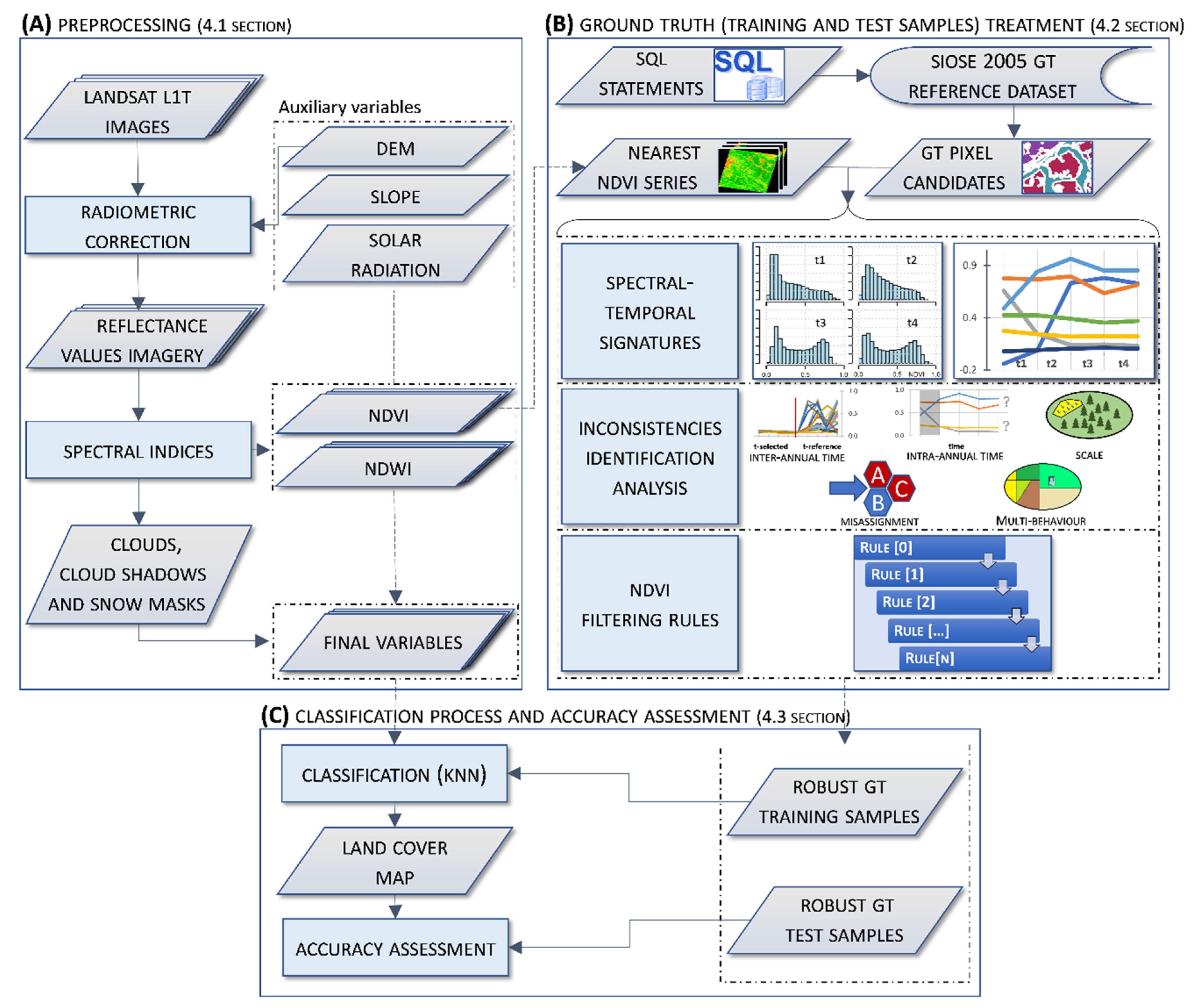
This study develops a framework to enhance land cover classification accuracy through quality control of GT areas based on a set of filtering rules. However, for these rules to be general and to fulfil the goal that other RS users achieve similar enhancement effects, it is important to explain the pre-processing of the imagery. The proposed filtering rules are based on analysing the NDVI time series. Choosing NDVI solves the usual GT reliability problems that occur in both the wilderness and crop categories, ensuring a likely phenological behaviour. This allows our method to be widely usable because the NDVI can be computed from almost all RS instruments. We evaluated the performance of the filtering rules through classification of study cases. The framework depicted in Figure 2 is divided into three main stages developed in the following subsections: (Section 4.1) image pre-processing and preparation of other auxiliary variables, (Section 4.2) ground truth (training and test samples) treatment, and (Section 4.3) classification process and accuracy assessment.

4.1. Image Pre-Processing

Satellite imagery was kept in the Universal Transverse Mercator 31 N zone, WGS84, spatial reference system in order to avoid introducing additional resampling problems. To generate a unified classification context, images captured on the same day (equal path/orbit) were mosaicked previously to any other process, using the Mosaic module of MiraMon. In other cases, a mosaic of neighbour dates was applied after radiometric correction to derive a coherent surface reflectance composition (see next point).

4.1.1. Geometric and Radiometric Correction

The satellite imagery had an L1TP level of processing (https://www.usgs.gov/core-science-systems/nli/landsat/landsat-levels-processing, accessed on 5 July 2021) based on ground control points and a DEM for topographic displacement correction. The average geometric Root Mean Square Error (RMSE) model was 5.55 m (median 5.26 m), 3.56 m for minimum and 10.39 m for maximum, for all images considered. Note that these figures mean an accuracy level clearly lower than half of a 30 m pixel.
Images were radiometrically corrected using pseudo-invariant areas following [83,84] the methods implemented in the CorRad module of MiraMon. The procedure obtains reflectance values from digital numbers through atmospheric and topographic corrections using, among other parameters, pseudo-invariant areas (PIA) derived from a long time-series of MODIS reference locations, sensor calibration parameters, solar illumination and cast-shadow models for each pixel and date.

4.1.2. Spectral Indices

Spectral indices are based on the properties of the spectral signatures that characterise the interaction of electromagnetic radiation with a specific surface. Combining several multispectral bands makes it possible to emphasise land cover characteristics, and identify where they dominate spatially. In this research, the legend was established based on previous studies [54], and describes thirteen categories: coniferous forest (CoF), broadleaf deciduous forest (BDF), broadleaf evergreen forest (BEF) shrublands (Shl), grasslands (Grl), bare soils (BrS), water bodies (WaB), urban areas and infrastructures (Urb), irrigated herbaceous crops (IHC), dry herbaceous crops (DHC), irrigated woody crops (IWC), dry woody crops (DWC) and, finally, rice crops (RiC). According to previous studies in the same geographical context, indices such as the Normalised Difference Vegetation Index (NDVI), the Normalised Difference Water Index (NDWI) or the Normalised Difference Snow Index (NDSI) have proven appropriate for emphasising vegetation phenological patterns, bare soils or water bodies, and also for excluding snow and cloud covers [54,81,85].
The NDVI [86] is the most widely used index for monitoring vegetation activity and its dynamics, and enables easy spatial and temporal comparisons. The index is derived as the difference values measured in red and near-infrared (NIR) bands, divided by their sum. The NDWI (NDWI3 in [87]) is used for identifying water bodies in classification processing. It is computed as the difference values measured in shortwave-infrared (SWIR) and NIR bands, divided by the sum of them. For all the dates considered, the NDVI and NDWI were used to better characterise many of the land cover classes in the classification process. Furthermore, the NDVI series were used to derive the filtering strategies carried out in Section 4.2.
Cloud-cover and cloud-shadow masking are a time cost, but they are a necessary pre-processing task. These areas were identified using the Fmask algorithm [88]. However, a visual review and manual corrections over the automatic procedure were required, mainly when masking thin clouds, contrails and anomalous sensor behaviours, the last of these being more common in earlier images.
The Normalised Difference Snow Index (NDSI) has a long history in the context of snow classification and uses the combination of SWIR and visible wavelengths [89,90]. It is assessed as the difference values measured in Green and SWIR bands, divided by their sum. We defined a threshold of NDSI > 0.15, lower than the usual 0.40 value [90], to discriminate snow-covered areas in line with other authors [91,92,93]. Decreasing the threshold gave better results when snow cover was discriminated in the Pyrenees, which has a rugged/irregular terrain and snow with a patchy distribution or mixed with vegetation. Once cloud or snow masks were derived, they were applied to exclude these areas from the spectral bands.

4.2. Ground Truth (Training and Test Samples) Treatment

In this study, GT (training and test) samples were extracted considering the SIOSE 2005 and 2011 datasets (SIOSE, https://www.siose.es/, accessed on 5 July 2021) [94] as a GT reference dataset source. We established and applied a set of Structured Query Language (SQL) statements to the SIOSE_CODE database field. The purest and high-cover-fraction polygons were identified, avoiding those that mix certain types of land covers (see Table S3 in the Supplementary Materials). Polygons were eroded, applying a 30 m buffering corresponding to Landsat pixel size, diminishing the influence of mixed pixels (heterogeneous) and the planimetric error associated with imagery/vectors at the boundaries [95]. Furthermore, polygons with an area ≤ 1.0 ha were discarded because of their low representativeness. The remaining polygons masked the initial set of GT candidate pixels evaluated for each category.
Given the extensive study area (four full Landsat scenes), some empirical tests were performed with different tile sizes (3 × 3, 5 × 5, 7 × 7 and 9 × 9) to define the best unit size of analysis, considering the trade-off between computation time and a better polygons subdivision. The selected option was partitioning polygons into tiles of 7 × 7 pixels (210 m wide) co-registered with the spatial pattern of the imagery. The Fishnet tool from the ArcGIS® 10.7 software (ESRI, Redlands, CA, USA) was used for tilling. This GIS technique makes it possible to partition large polygons into homogeneous square-shaped sub-polygons for sampling purposes, reducing the spatial autocorrelation and increasing the homogeneity in the spatial distribution of the TTA subset used for modelling. For each category, we randomly selected 70% of the total area for training and preserved the remaining 30% for validation purposes, ensuring category representativeness in both subsets. Tiles were also helpful for estimating statistics locally (central tendency and statistical dispersion measures) to define filtering rules. Final polygon masks defined the initial GT candidate pixels for each category.
In the exploratory phase, the LCM-2002 imagery was selected because of its temporal proximity to SIOSE 2005 rDS. The classification imagery should describe the intra-annual phenology during the growing season of natural and agricultural land covers. Dates spanning from Spring to Autumn enhance the phenological contrasts of categories (Table S2). Images were pre-processed, cloud masked, and the radiometric correction performed before deriving the NDVI series.
As a form of sensitivity analysis, we evaluated the performance of the rules by using the SIOSE 2011, as a new rDS, and contemporary imagery, deriving the LCM-2012. Complementarily, rules performance was evaluated in a new spatial context, the scenes 200-032 and 200-033 considering SIOSE 2005 as rDS.

4.2.1. Spectral-Temporal Signatures

The training set of polygons (70% of the GT total area) were masked with the NDVI series, and their temporal dynamics were evaluated. The objective was to analyse phenological patterns of each category in order to identify abnormal behaviours. Furthermore, analysing the temporal patterns served to formulate filtering rules and approximate the parametrisation of the rules.
Inconsistencies were identified through the temporal frequency distribution as in the plots in Figure 3. For instance, low NDVI values were observed in coniferous, broadleaf evergreen, and deciduous forest because of the associations among several categories within polygons.
Furthermore, bimodal distributions were identified in the case of broadleaf evergreen forest and irrigated herbaceous crop categories. The inconsistencies were analysed, and filtering rules applied to exclude them. Histograms of the rest of the categories are detailed in Figure S1 in the Supplementary Materials.

4.2.2. Identification and Analysis of Inconsistencies

Historical PNOA orthophotography (dates between 1998–2003) and the imagery spectral bands supported phenological interpretation during the analysis. Furthermore, the National Forest Inventory (NFI) (version 2 (1986–1995) and version 3 (1997–2007)) provided robust information about forest species composition in the inventory plot locations over time [97]. SIOSE datasets provide particularly valuable and useful cartographic information for the Spanish territory; however, the complexity of the territory and land cover dynamics makes it necessary to have an appropriate set of filtering measures to avoid inconsistencies in the TTA. Some of the sources of the identified inconsistencies were:
(a)
The inter-annual time difference between the rDS and imagery dates. There is a temporal lag between rDS and LCM-2002 imagery. Figure 4 depicts the NDVI temporal activity of several irrigated herbaceous crop patches (tiles) where no photosynthetic signal is detected during the summer dates of the years previous to 2005. Dry herbaceous crops or fallow practices were predominant in this area before irrigation plans were implemented in this geographic context. The set of patches occupies 787 ha, resulting in a significant error source that affects the identification of irrigated and dry herbaceous crop classes.
(b)
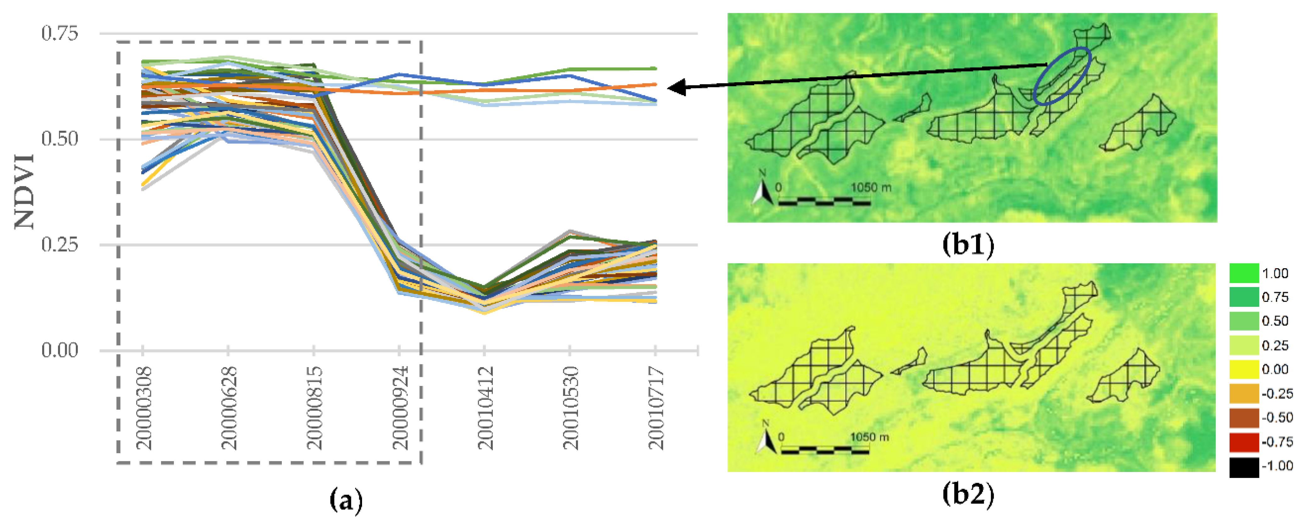
The intra-annual time series collect annual phenology, which is constrained by the availability of the imagery. Some intra-annual events (forestry clear-cutting practices and fire disturbances) causes abrupt phenology changes at an intra-annual time scale. These events should be managed (selected/excluded/reclassified) in GT candidate samples. In Figure 5, a forestry clear-cutting practice in a coniferous plantation is shown; the coniferous phenological activity drops on 24 September 2000, affecting an area of 176 ha. The polygons that are not affected show a steady temporal profile.
(c)
Scale errors are associated with the conflict between the rDS minimum mapping unit (SIOSE with values of 0.5, 1 or 2 ha, depending on the cover type) and the Landsat spatial resolution (30 m). SIOSE composite land cover polygons circumscribed different phenological responses in the imagery resolution, as shown in Table 1. Figure 6 shows a composite land cover polygon with an association of 70% coniferous, 20% pasture and 10% shrublands. Coniferous forest and sparsely vegetated plots can be identified in the orthophotography on 28 April, 2001, NDVI, where the lower values are pastures/grasslands.
(d)
Labelling errors in rDS feature labels can be due to the subjectivity of photointerpretation or human errors when the polygons label are assigned. Figure 7 shows an almost pure polygon defined as an association of 95% broadleaf evergreen forest and 5% shrublands. Despite its definition, the observed phenology conforms to deciduous patterns. In (a), a dense forest structure can be recognised, which corresponds with dominant deciduous species (Fagus sylvatica, Quercus pyrenaica) inventoried in the NFI plots. In (b) and (c), 28 April 2001, and 25 July 2001, NDVI showed a clear increase in NDVI values between the dates. The polygon occupies 198 ha, which can become a source of characterisation errors between evergreen and deciduous forest classes.
(e)
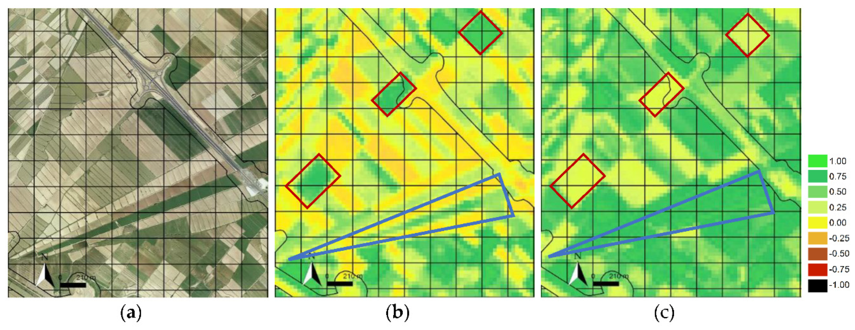
Multiple (phenological) behaviours are mainly associated with agriculture categories. Crop phenology is complex, and there is a large chance that two neighbouring crop fields within a polygon can be in very different phenological stages (active crops, fallow patterns), as well as belong to different categories (winter crops, summer crops or woody crops). Examples of multiple behaviours were detected in dry and irrigated herbaceous crop polygons. The latter is exemplified in Figure 8. Only part of the entire polygon is displayed due to the large area occupied by the irrigated crops in this area. In (a), the orthophotography depicts the spatial variability, different sizes and phenological states of crop fields. In (b), 28 April 2001, NDVI denotes active winter (red rectangles), perennial crops and other inactive fields. In contrast, on 25 July 2001, NDVI denotes that (c) active summer crops (blue triangle) and inactive fields dominate the area. The contrasting phenological behaviours in large irrigated crop polygons become a source of error and confusion between winter/summer crop categories.

4.2.3. NDVI Filtering Rules

Filtering rules aim to minimise the impact of errors in GT samples used for classification. The rules were generated to deal with issues observed during the exploratory phase and were constructed based on the previous analysis of spectral-temporal signatures, which serve to identify the phenological patterns of each category. The phenological patterns were analysed considering NDVI, but other vegetation indices could be used if their usage suggests an even better behaviour. We considered the LCM-2002 imagery in the examples of the rules below.
Rule 1: Maximum NDVI temporal response
This rule serves to select pixel locations with the maximum NDVI temporal response, dynamically and in each tiled polygon. The rule is defined as:
NDVImax ≥ | ≤ (Max r1_μ_tile ± Max r1_σ_tile), r1_μ ∈ [−1,1], r1_σ ∈ [0,1]
where NDVImax is the maximum value per each pixel in the imagery series and is taken as a reference value in a per-pixel evaluation form. Individual pixels are evaluated regarding two statistics calculated at a tile-polygon level; (1) the r1_μ_tile is a central tendency measure (e.g., median (MED)) evaluated for each tile-polygon and date; the maximum of the central tendency of the series determines the Max r1_μ_tile value; (2) the r1_σ_tile is a dispersion measure (e.g., the standard deviation (SDV) on the means of the absolute differences from the median) calculated for each tile-polygon and date; the maximum dispersion of the series determines the Max r1_σ_tile value. Therefore, each tile-polygon is characterised by the maximum central tendency value, the median, and the maximum dispersion measure, the dispersion measure for all the dates. Pure SIOSE simple land cover polygons are expected to be characterised by a median and a relatively low dispersion measure. However, in composite land cover polygons with a mixture of categories, the dispersion measure varies according to the tile composition variability. For a dispersion measure, the cut-off value defined by the Max r1_μ_tile ± Max r1_σ_tile can be displaced towards lower or upper NDVI values to determine the acceptable variability for the category.
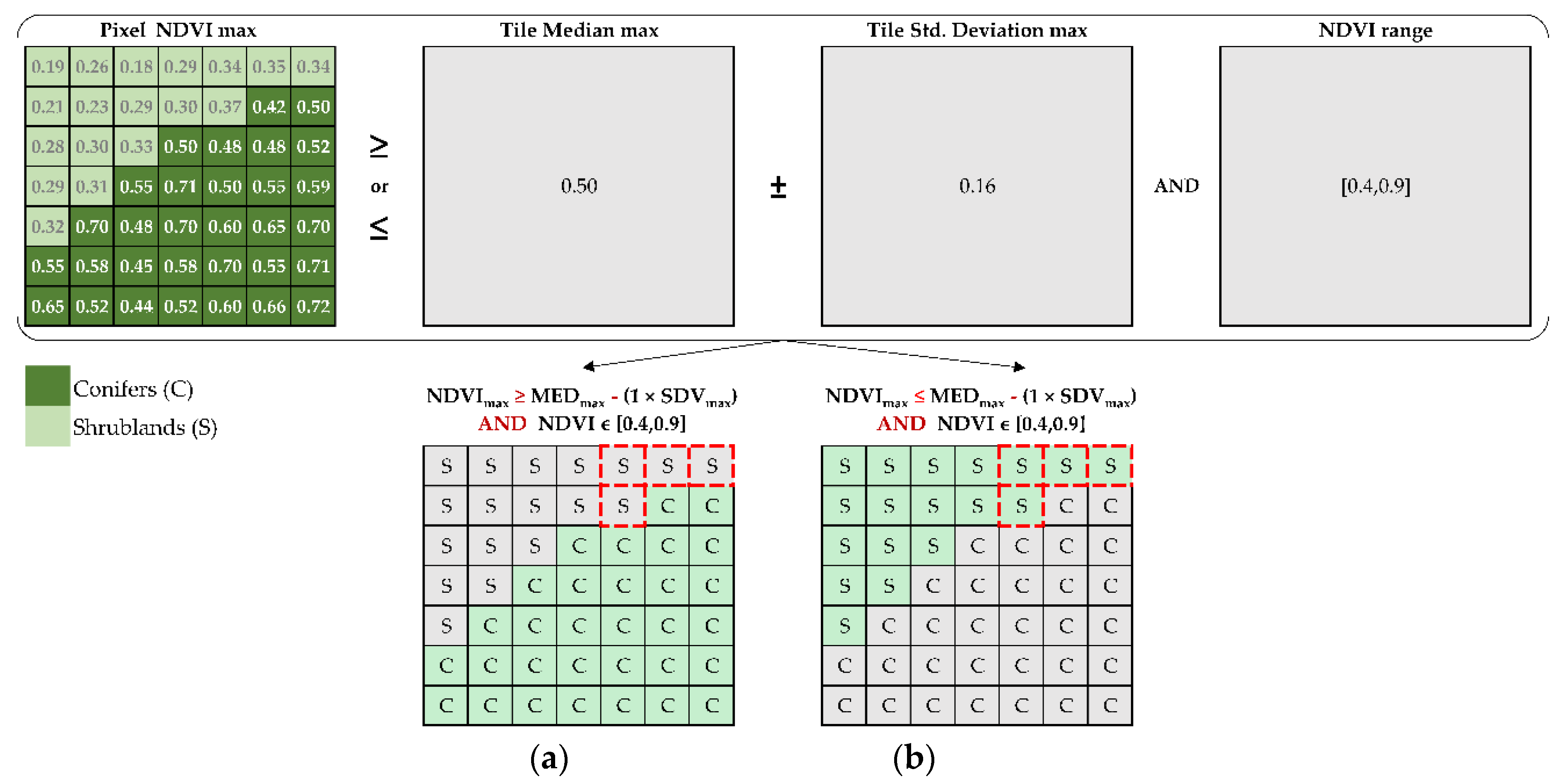
For instance, we focus on a composite land cover polygon tile (e.g., A(65CNF_35MTR)), defined as an association of 65% coniferous and 35% shrubland in Figure 9. In this tile, coniferous pixels can be discriminated by selecting pixels with an (NDVImax ≥ MEDmax − (1 × SDVmax)). Complementarily, pixels with an (NDVImax ≤ MEDmax − (1 × SDVmax)) characterised low NDVI values associated with shrublands. In both statements, transitional values (red squares) would be incorrectly managed if they were not filtered out.
This rule is appropriate for wilderness land cover categories but is also extendable to agriculture categories. The rule makes it possible to discriminate forest categories (e.g., coniferous) from non-forest vegetation categories (e.g., shrublands), and also differentiate between the non-forest vegetation categories in the natural succession, especially in composite land cover polygons. Used together with Rule 2, it has the benefit of defining the range of NDVI values over which a category varies. Thus, this rule is useful for avoiding scale errors and intra-annual errors, specifically in composite land cover polygons where several categories and transitional NDVI values coexist. Some categories require selecting the lower NDVI response, such as bare soils, considering an NDVImax ≤ MEDmax + (1 × SDVmax).
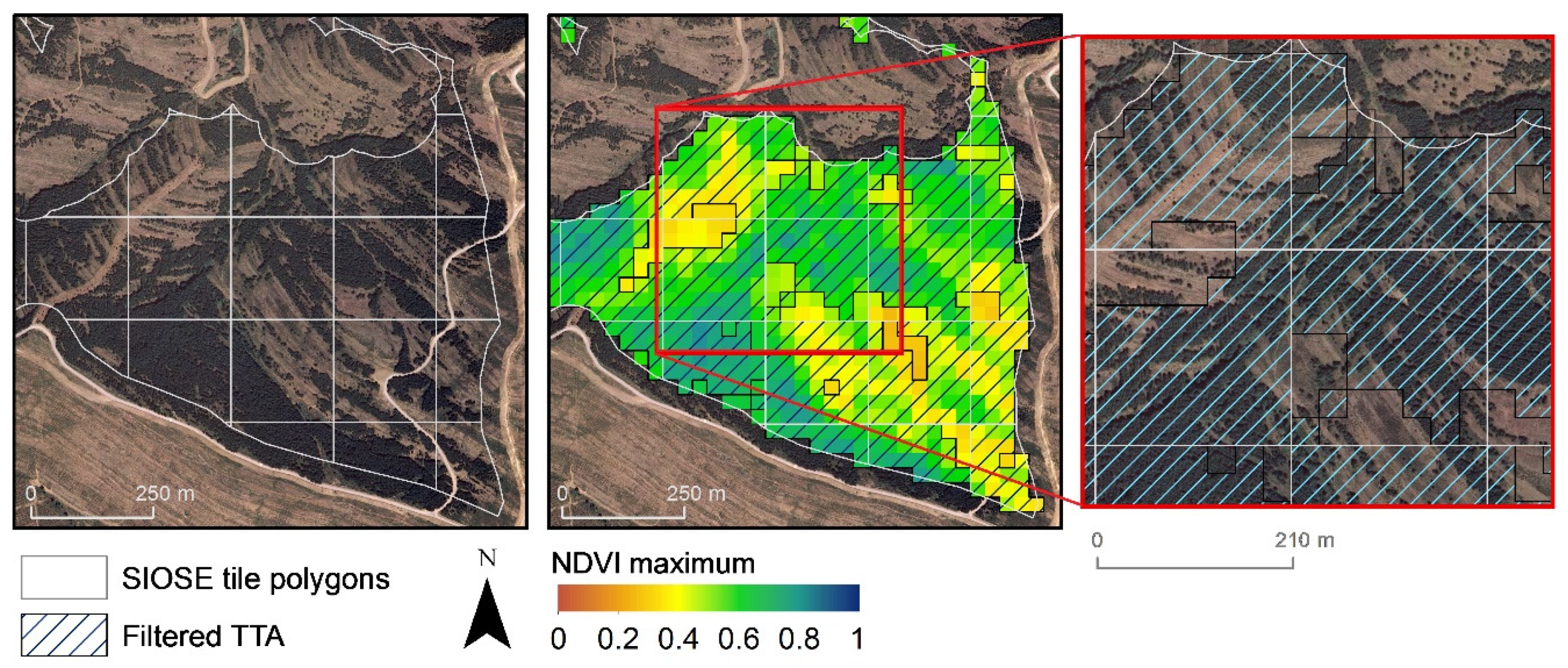
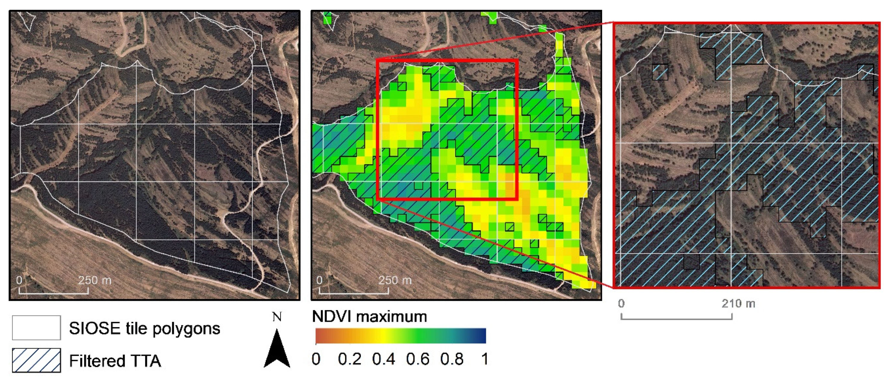
Rule 1 is applied over a composite land cover polygon defined as an association of 70% coniferous and 30% shrubland depicted in Figure 10. The rule statement is defined as (NDVImax ≥ MEDmax − (1 × SDVmax)) to select the more densely forested areas. The orthophotography allows us to differentiate compact and densely forested plots from sparsely vegetated areas. Tile polygons are depicted with white outlines. The highest NDVI maximum values are shown from green to blue, whereas the values under ~0.40 are associated with scarce vegetation. The zoom details pixel exclusion in these areas. It is worth noting that for the tiles where lower NDVI maximum values predominate (e.g., tiles mixing coniferous and shrubland or those affected by a forest fire), it is essential to consider a complementary condition statement to exclude lower NDVI responses, the minimum NDVI threshold detailed in Rule 2.
Rule 2: NDVI range along with the ‘n’ dates
This rule determines the range of NDVI values over which a category varies along the ‘n’ dates considered. The rule is defined as:
∀ NDVI ∈ [r2_a,r2_b]; r2_a,r2_b ∈ [−1,1]
where r2_a, r2_b are the NDVI minimum and maximum values, respectively, which define the NDVI range of variation of a category. Considering the conceptual example shown previously in Figure 9, Rule 2 was added to manage transitional behaviours, which is exemplified in Figure 11. The sentence is defined as: (NDVImax ≥ | ≤ MEDmax − (1 × SDVmax) AND (∀ NDVI ∈ [0.40,0.90])), where values outside the limit are excluded.
This rule complements Rule 1 but can also be used independently. Since the series of NDVImax is assumed as a reference value, a minimum NDVI threshold is necessary. The aim is to isolate positions that do not fit the category NDVI characteristic range in the initial set of GT candidate pixels, especially in composite land cover polygons. Moreover, intra-annual disturbance events (forestry clear-cuttings or fire events) in forested areas cause NDVI drops, for which pixels can also be isolated. Rule 2 used independently can be helpful to extract crop categories characterised with a specific NDVI range of values (e.g., rice crops NDVI range approximately between [−0.30,0.80]).
Locations in Figure 10 with low NDVI values were not adequately filtered. Rules 1 and 2 were applied in the exact location, and the results are displayed in Figure 12. Excluding non-forested locations and anomalous minimum values requires defining a threshold (NDVI minimum) in accordance with the category variability. The filtering statement is defined as (NDVImax ≥ MEDmax − (1 × SDVmax) AND (∀ NDVI ∈ [0.40,0.90])). Those pixels under the NDVI < 0.40 are discarded (any disturbance events causing NDVI drops, sparsely vegetated or low-density forested areas, shrublands, pastures, bare soils or even water bodies), so that only densely forested plots remain.
Rule 3: Photosynthetic activity for ‘n’ dates
This rule is a proxy of the total photosynthetic activity for a category considering the range of values over which the sum of ‘n’ dates NDVI variates. The rule is defined as:
i=(1,n) NDVIi ∈ [r3_a,r3_b]; r3_a,r3_b ∈ [−n,n]
where r3_a and r3_b are the minimum and maximum values between which the total sum (NDVIsum) of ‘n’ NDVI varies for a category. It works at the individual pixel level.
The rule makes it possible to discriminate between active and non-active agriculture crop fields in herbaceous and woody crop categories. Since the rule amplifies the NDVI total signal, it enables better recognition between active/non-active crops within dry or irrigated crop categories in the SIOSE dataset. Defining thresholds to discriminate irrigation regimes favours deriving consistent TTA sets for LCM time series production, and hence, more reliable land cover change analysis in these categories, mainly in irrigated woody crops, where there is also a mixture with dry crops. For the forest categories, the rule is useful for distinguishing the most active broadleaf deciduous species, especially those located close to rivers.
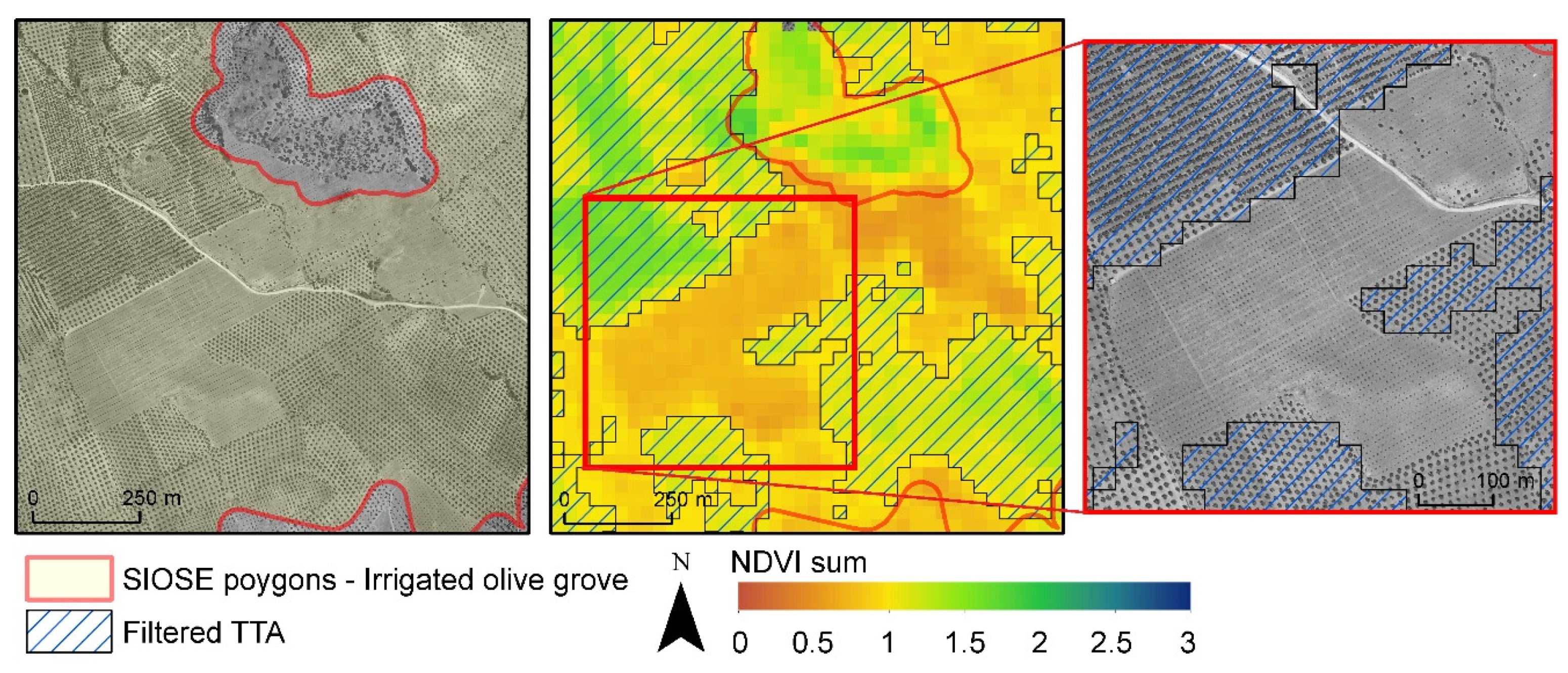
We applied this rule in irrigated olive grove plantation polygons, shown in Figure 13. Orthophotography with a 2001 date can be used to identify consolidated and productive parcels close to recent plantation fields, besides their total photosynthetic activity correspondence values. Through visual interpretation, we defined the NDVI sum ∈ [1.0, 2.0] to capture dense plantations, discarding the lower photosynthetic response associated with recent plantations and non-cultivated areas.
Rule 4: Contrast between NDVImax values of a group of dates
The intra-annual phenology variability is characteristic for each category. The rule is based on the NDVI maximum difference between the initial and final growing season, typically the summer and spring dates, but is adaptable to other dates or groups of dates. The rule is defined as:
NDVIdifference (NDVImax Summer dates − NDVImax Spring dates)
∈ [r4_a,r4_b]; r4_a,r4_b ∈ [−2,2]
where r4_a, r4_b are the minimum and maximum values derived from the absolute difference between the NDVImax reached on the summer and spring dates. The NDVI difference can also be interpreted as the NDVI temporal gradient between two temporal moments.
The rule makes it possible to control more dynamic agronomic classes and forest behaviours. Considering the summer and spring NDVI maximum differences, it is well known that there is a strong positive temporal gradient during the growing season, characteristic of summer crops (herbaceous or rice crops), deciduous forest species (Fagus sylvatica and sclerophyllous deciduous and pseudo-deciduous species) and some woody crops (vineyards). In contrast, the strong negative gradients are typically associated with winter crops or low-altitude pastures. Other categories (e.g., coniferous, broadleaf evergreen forest, shrublands or urbanised areas) depict a temporal response with no trend in the NDVI temporal profiles, which means close to zero NDVI temporal gradients. This rule distinguishes polarised phenological patterns as winter and summer crops or deciduous and evergreen forest patterns and allows each category to be characterised with the NDVI temporal gradient. However, the rule is limited when less contrasting patterns are discriminated (between bare soils and fallow lands or between coniferous and evergreen forest categories). Furthermore, the rule helps to define the NDVI temporal gradient patterns. This avoids labelling misassignment or other errors related to rDS and inter-annual time differences in imagery when rapid transformations occur (e.g., dry to irrigated regimes and forest conversion from evergreen to deciduous species, or vice-versa). The rule can also be used to discriminate mixed forest in regular pattern associations when deciduous with evergreen patterns coexist.
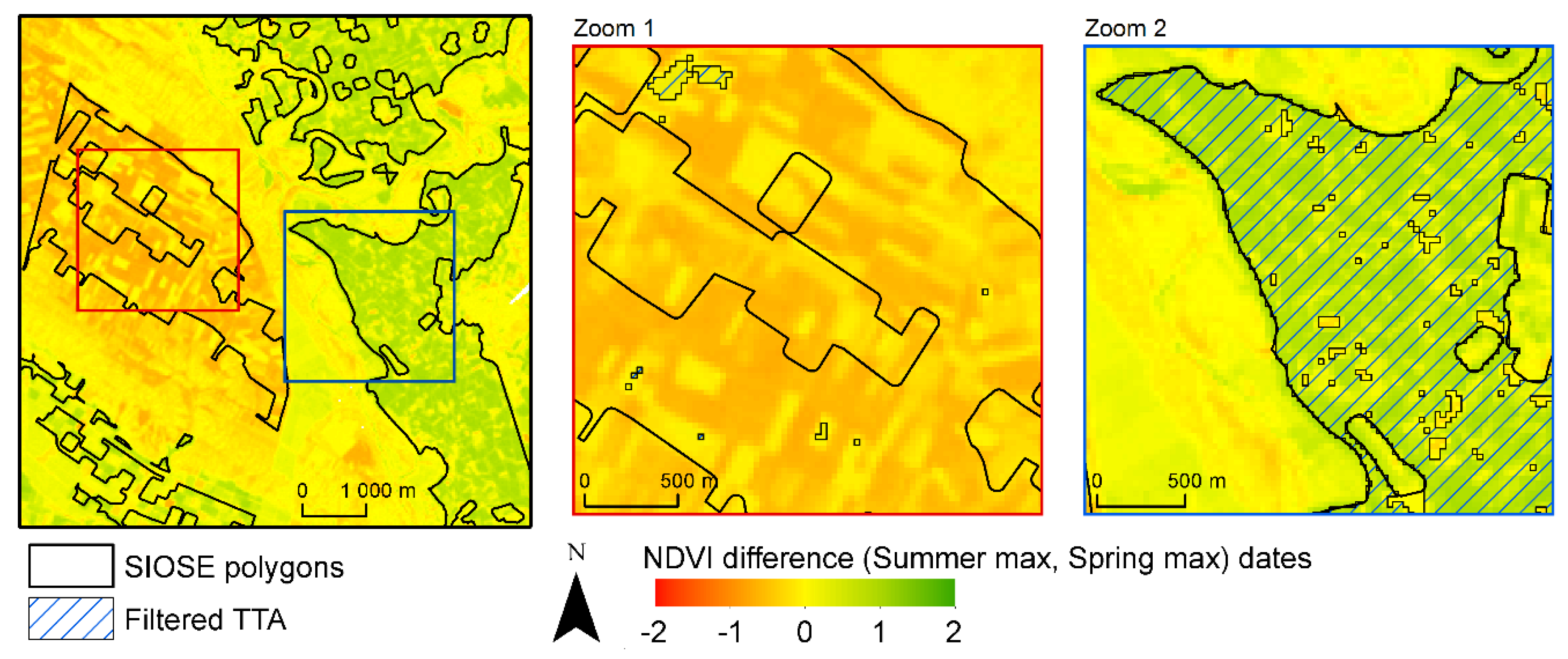
The example in Figure 14 illustrates a labelling inconsistency associated with the rDS and the inter-annual difference of the imagery. The polygon label is defined as irrigated herbaceous crops, while the real phenology revealed winter crops or fallow patterns related to agriculture practices of dry herbaceous crops. Rule 4 was established and applied to exclude the negative temporal patterns in the initial candidate pixels of irrigated herbaceous crops. We approximate the NDVI absolute difference range values between [0.05, 2] based on the local analysis of the pixels involved. Limits should not be restrictive since the aim is to only exclude the negative NDVI temporal gradients.
Rule 5: Phenological moment
Establishing NDVI thresholds on specific dates or a group of dates or direct comparisons between dates or a group of dates may be required. Some casuistics are:
NDVI Spring date or, NDVI max|min Spring dates ≥ | ≤ r5_a
NDVI Summer date or, NDVI max|min Summer dates ≥ | ≤ r5_b
NDVI Autumn date or, NDVI max|min Autumn dates ≥ | ≤ r5_c
NDVI max|min Spring dates ≥ | ≤ NDVI max|min Summer dates
NDVI max|min Summer dates ≥ | ≤ NDVI max|min Autumn dates
NDVI max|min Spring dates ≥ | ≤ NDVI max|min Autumn dates,
r5_a,r5_b,r5_c ∈ [−1,1]
where r5_a, r5_b, r5_c are specific NDVI thresholds in phenological moments defined for a particular date or group of dates. For instance, to detect rice fields, we can establish a threshold in NDVI spring dates ≤ 0.0 together with high activity during the NDVI summer dates ≥ 0.60. Direct comparisons (NDVImax spring dates ≥ NDVImax summer dates, useful for winter crop characterisation) between dates or a group of dates can also be used for better phenological control. It is a flexible rule that makes it possible to compare a free combination of NDVI thresholds between dates.
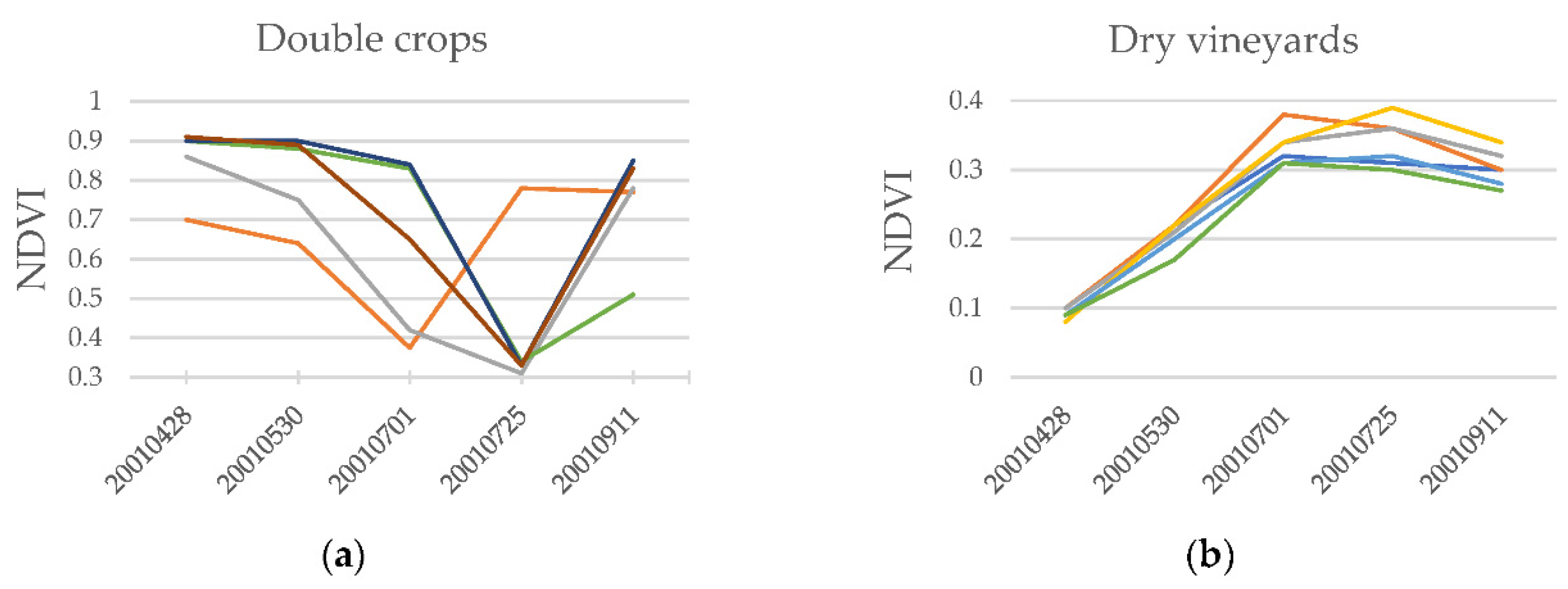
Specific situations require NDVI thresholds to analyse particularly tricky phenological patterns. For instance, when there are two relative minimum (or two maximum) NDVI values in an NDVI temporal profile. The rule helps establish specific NDVI thresholds to reproduce temporal profiles in specific categories on which the map producer focuses their interest. For instance, detecting the temporal pattern of double crops requires establishing an NDVI minimum at the moment of harvesting and two maximum values on early spring and later summer dates. Furthermore, this rule is helpful for managing vegetation senescence in temporal profiles.
Figure 15 represents examples where double crops and dry vineyard patterns were extracted from irrigated herbaceous crops and dry vineyard woody crop polygons. Rule 5 in double-crop patterns was defined as [NDVI20010428 ≥ 0.50] AND [NDVImin summer ≤ 0.40] AND [NDVImax summer ≥ 0.50], which makes it possible to capture the variability of the crop in the summer dates. For characterising active dry vineyard plantation fields, Rule 5 was defined as [NDVI20010428 ≤ 0.15] AND [NDVImax summer ≥ 0.30] AND [NDVI20010701 > NDVI20010911], adapting the rule to capture the characteristic senescence period of the crop.
We defined the statements of the filtering rules and proposed a parametrisation for each category, adapted to the geographical context, detailed in Table S4 in the Supplementary Materials. The initial set of candidate pixels was filtered based on the rules, deriving a robust set of TTA, which were randomly selected to be used in the classification stage.

4.3. Classification Process and Accuracy Assessment

We used the k-nearest neighbour (kNN) classifier implemented in MiraMon, parallelised for better performance, to derive LCM over which we evaluated the performance of the filtering rules. kNN is a supervised classification approach that relies on labelled input samples to learn and produce an output in the new given unlabelled data. The process is developed in two steps for each pixel in the image: (1) the algorithm determines the nearest neighbours by calculating a distance metric (e.g., the Euclidean distance) between the target pixel and each training area provided; then (2) the target pixel label is determined by selecting the kNN candidates (defined by the map producer), over which the modal category is calculated. The kNN parameter was fixed to 15, based on a previous work analysis and considering better robustness when the number of training samples is large [54], as it is in the context of two Landsat scenes.
The variables used in the classification process were Landsat TM and ETM+ bands 3, 4, 5 and 7, OLI bands 4, 5, 6 and 7 for each date, as well as two indices (NDVI, NDWI) and three topo-climatic variables (altitude, slope and summer potential solar radiation). Thermal bands were excluded, and Blue and Green bands were discarded because of their high correlation and the strong influence of atmospheric aerosols. The spectral bands, spectral indices, slope, altitude and summer potential solar radiation were all scaled to 0–100 so that values were all unified in the same range. In total, the classification dataset in all study cases was composed by thirty tree variables.
The map accuracy was assessed by evaluating the agreement between the map produced and the test areas, summarising the discrepancies by means of the confusion matrix [40,98,99]. The confusion matrix is essential for quantifying the impact of the TTA error on the map accuracy and the performance of the filtering rules. The unequal presence of classes in our map obliges us to adapt some computations. For instance, if the commission errors of dry herbaceous crops are associated with the bare soils category, but the number of herbaceous crop test samples is considerably larger than the bare soils test samples (e.g., one order of magnitude as the first ones are much more frequent in the area), then the interpretation of the user’s accuracy is incorrect. This could be balanced before the confusion matrix calculations; however, this implies losing test samples and deciding where to remove them. Alternatively, it can be corrected by a factor computed as follows:
Factor   i   = ( Map   pixels   i / Map   total   pixels ) / ( Test   pixels   i / Test   total   pixels )
where, ‘i’ denotes each category. The factor computed for each category allows us to obtain a confusion matrix free from these imbalances.

5. Results

The LCM generated for the four temporal cases (LCM-1987, LCM-2002, LCM-2012 and LCM-2017) and the additional spatial case are shown in Figure S2, and their confusion matrices are detailed in Tables S5–S14 in the Supplementary Materials. For simplicity, only LCM-2002 results are detailed due to the coherence with the rest of the maps generated. The performance of the rules is detailed through visual examples, and their confusion matrices are interpreted in the following subsections.

5.1. The Performance of the Rules in Visual Examples

The visual examples in Figure 16 and Figure 17 illustrate the performance of the rules in specific locations. The LCM-2002 classifications were compared before and after the rules were applied.
Example A in Figure 16 represents Rules 1 and 2 applied to coniferous polygons to prevent the scale and intra-annual time errors. Rule 1 selected all the most active positions in the period according to the (NDVImax ≥ MEDmax − 1SDVmax) evaluated in tiles, avoiding the lowest NDVI responses (shrublands, grasslands, bare soils) typically associated with SIOSE composite polygons. Rule 2 ensured that NDVI values varied within the range of variation allowed for the category (e.g., ∀ NDVI ∈ [0.40, 0.90] for coniferous forest) on all dates. The clear-cutting event was misclassified as coniferous forest using unfiltered TTA, but correctly classified as shrublands when the filtering rule was applied.
Example B in Figure 16 exemplifies a misassignment error, where pixels on a broadleaf evergreen forest polygon depict a clear deciduous pattern. Rule 4 served to exclude pixels with deciduous temporal patterns in the evergreen category. The statement rule concatenates three terms: (NDVImax ≥ MEDmax − 1SDVmax) AND (∀ NDVI ∈ [0.40, 0.90]) AND (NDVI difference ∈ [−0.15, 0.05]), which allow us to extract the most active forested areas (Rules 1 and 2), and avoid deciduous (positive NDVI gradients) patterns (Rule 4). The classification results showed a mixture of evergreen and deciduous forest classified pixels when unfiltered TTA was used, while the filtered set provided pixels correctly classified as deciduous forest.
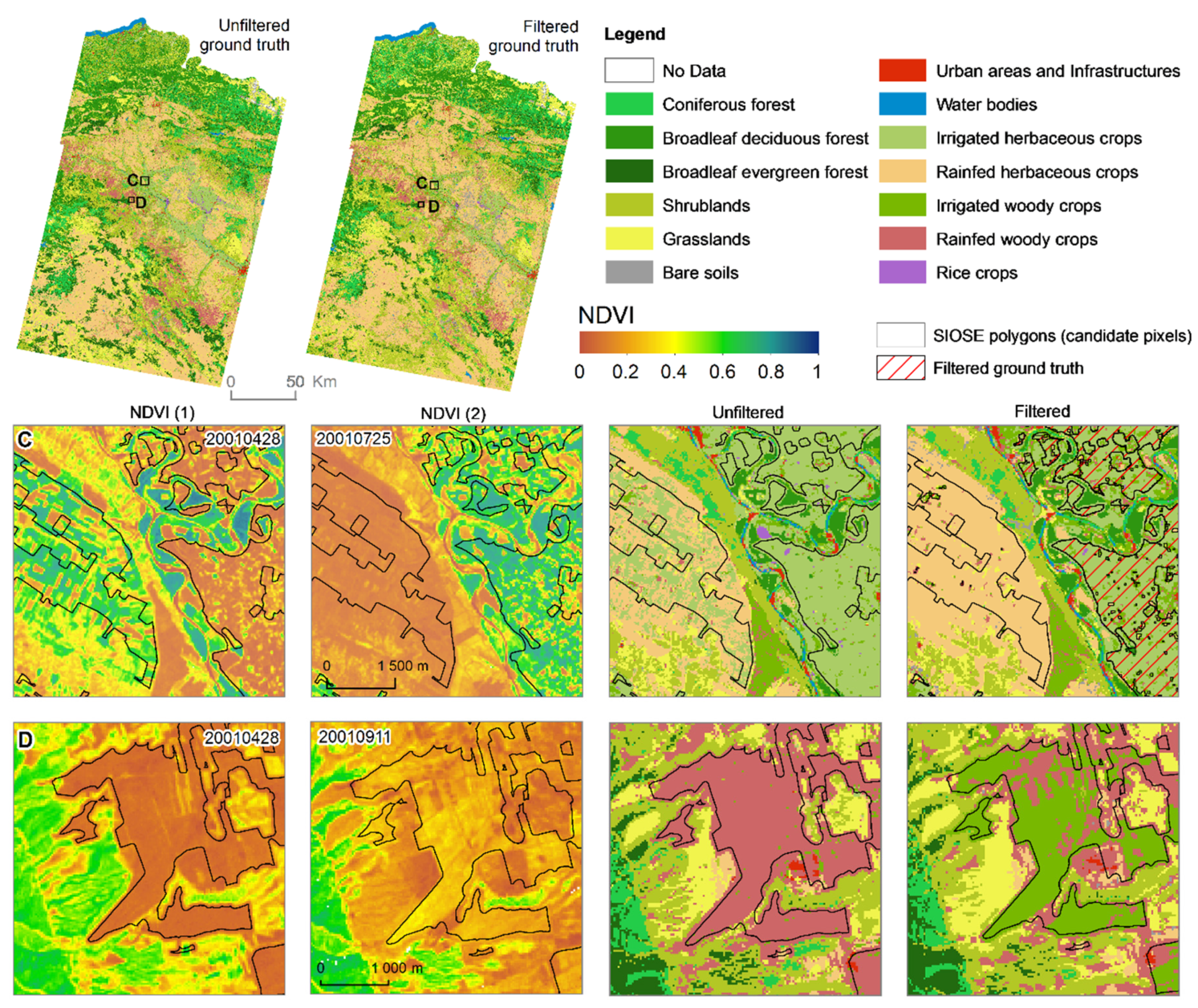
Example C in Figure 17 illustrates an inter-annual time error. Several irrigated herbaceous crop polygons depicted phenological patterns associated with dry herbaceous crops. Rule 4 was used to characterise the irrigated crops: a positive NDVI gradient during the growing season, excluding any negative NDVI gradient associated with the dry crops. The rule statement was defined as (∀ NDVI ∈ [0.05, 0.90]) AND (NDVI difference ∈ [0.05, 2.00]), capturing the irrigated crops with a positive NDVI temporal gradient. The results showed the area misclassified as irrigated herbaceous crops when unfiltered TTA was used, while the filtered set correctly classified the area as dry herbaceous crops.
Example D in Figure 17 describes the existence of multiple behaviours in woody crop categories. In the example, dry vineyard woody crop polygons depict anomalously high photosynthetic activity (related to irrigated woody crops) with irrigation ponds located in parcels.
The rule statement defined for dry woody crops was (∀ NDVI ∈ [0.05, 0.60]) AND (NDVIsum ∈ [0.30, 0.75]) AND (NDVIdifference ∈ [0.15, 1.00]) AND ([NDVI max Spring] < [NDVI max Summer]). The first term made it possible to capture the NDVI range of variation; the second term, made it possible to determine the minimum total photosynthetic activity as a dry woody crop; and the third and fourth terms characterised the positive NDVI difference during the growing season. This made it possible to exclude any pixel contamination with herbaceous crops or pastures, which generally have negative NDVI difference patterns. Unfiltered TTA resulted in misclassifying the area as dry woody crops. Using filtered TTA, the level of NDVI total activity reached in these locations allowed us to classify them as irrigated woody crops.

5.2. The Performance of the Rules in Confusion Matrices

The results of the confusion matrices, comparing unfiltered and filtered TTA for LCM-2002, are detailed in Table 2 and Table 3. The LCM-2002 overall accuracy (OA) using unfiltered TTA was 83.8% and 88.6% when it was weighted by the ground truth area considering only classified pixels (OAw). For the filtered TTA, the OA reached 93.0%, and OAw obtained 96.0%. Therefore, matrices corroborated a better identification of categories when the filtering rules were applied, decreasing the confusion between classes and avoiding error inconsistencies. This pattern could also be seen in the rest of the LCM.
Figure 18 compares the omission error and the commission error resulting from the evaluation of the maps with and without applying the filtering rules. There is a clear reduction in OE and CE in all categories.
Wilderness land cover categories (coniferous forest, broadleaf evergreen forest, broadleaf deciduous forest, shrublands, grasslands and bare soils) showed a clear reduction in both OE and CE. This pattern was expected due to the more stable phenological patterns in wilderness categories and the effect of minor inter-annual time problems. The coniferous forest showed errors associated mainly with broadleaf evergreen forest, shrublands, and, to a lesser extent, broadleaf deciduous forest. The application of Rules 1 and 2 reduced the scale errors (the association of forest with the shrubland, grassland, and bare soil categories) and intra-annual errors (disturbance events), while Rule 4 served to exclude labelling misassignments (coniferous polygons mislabelled as deciduous forest). This led to a reduction in OE from 18.0% to 12.9% and in CE from 7.3% to 2.7%. However, the OE for coniferous forest and broadleaf evergreen forest remained, which shows that a mixture of the two categories in filtered TTA remains to a certain extent.
Broadleaf deciduous forest errors were associated with broadleaf evergreen forest and shrublands. Rules 1 and 2 were helpful for reducing the scale errors, and Rule 4 made it possible to exclude temporal responses without trend NDVI temporal patterns. This reduced the OE from 7.3% to 2.5% and the CE from 8.0% to 2.1%. Broadleaf evergreen forest errors were mainly related to shrublands and broadleaf deciduous forest. Rules 1 and 2 served to reduce the scale errors, and Rule 4 helped exclude deciduous patterns. When the filtering rules were applied, the confusion matrices reported that the OE dropped from 9.1% to 5.0% and the CE from 20.7% to 15.2%.
Shrublands were confused mainly with grasslands and broadleaf evergreen forest, dry herbaceous and dry woody crops. Confusion matrices revealed a decline in the OE from 20.1% to 7.7% and in the CE from 17.2% to 9.7%. Shrublands are characterized by high intraclass variability in the study context. The rules aim to capture the intraclass variability with Rules 1 and 2 and limit the NDVI temporal gradient with Rule 4, excluding deciduous patterns associated with grasslands or deciduous forest species. Once the rules have been applied, there is still confusions with dry woody crops. Grasslands were confused mainly with shrublands, dry herbaceous crops, and dry woody crops. The confusion matrices revealed a reduction in the OE from 16.0% to 10.8% and in CE from 23.7% to 10.6%. Rules applied to grasslands were defined to capture humid and dry phenological patterns separately, where Rules 1 and 2 capture a wide range of variation and Rules 4 and 5 serve to define NDVI gradients and restrictions of phenological moments. Nevertheless, after the rules have been applied, there are still some confusions with the dry woody crop category.
The bare soils category was confused mainly with grasslands, dry herbaceous crops and dry woody crops. Rules 1 and 2 were applied to capture low NDVI responses, and Rule 4 to restrict the steady NDVI gradient. Confusion matrices showed a significant drop in the OE from 49.9% to 12.0% and in the CE from 43.4% to 18.2%. Urban areas and infrastructures were confused with bare soils and dry herbaceous crops. Confusion matrices showed a drop in the OE from 32.5% to 18.9% and in the CE from 20.1% to 7.2%. The water bodies category was confused with several categories, but due to their characteristic shortwave infrared absorption and negative NDVI values, Rule 2 was sufficient for filtering this category correctly. The OE dropped from 18.1% to 0.0% and the CE from 3.5% to 0.0%.
Irrigated herbaceous crops were confused mainly with dry herbaceous crops and irrigated woody crops. Error related to dry crops was associated with the inter-annual time difference between the rDS and the imagery date, so that the phenological patterns of the winter crops and summer crops are mixed in the polygons. Once pixels with the dry patterns were decreased using Rule 4, the OE dropped from 24.3% to 6.9% and the CE from 21.2% to 3.2%. Resolving this inconsistency in irrigated herbaceous crops also had an effect on the accuracy of classifying dry herbaceous crops. Dry herbaceous crops were confused with irrigated herbaceous crops and grasslands and to a lesser extent with dry woody crops. Once the inconsistencies with irrigated crops were decreased by using Rule 4, the OE dropped from 10.8% to 5.8% and the CE from 7.9% to 1.9%. Rice crop confusion errors were related to irrigated herbaceous crops, which share common phenological patterns (positive NDVI gradient and high photosynthetic activity). The OE dropped from 20.3% to 0.5%, while the CE decreased from 34.1% to 17.3%.
Irrigated woody crops and dry woody crops are characterised by mixtures of different photosynthetic activities and soil contributions in crop fields. Based on the proxy of the photosynthetic activity, Rule 3 aimed to bring order to the greenness level achieved in different types of woody crops. This strategy excluded new plantations or even cases of irrigation plans not established on the imagery date. The OE associated with irrigated woody crops dropped from 38.6% to 3.8%, and dry woody crops did the same from 27.8% to 5.9%. The CE dropped from 45.3% to 9.8% for irrigated woody crops and from 24.8% to 10.8% for dry woody crops. The figures show a reduction in confusion with categories other than woody crops but an increase in the commission error with shrublands and grasslands, which to a certain extent share common patterns with the spectral variability of dry woody crops.
The LCM-1987 and LCM-2017 were derived considering GT samples generated from the SIOSE 2005 rDS. The results in the confusion matrices depicted a similar reduction in OE and CE in the categories, and more significantly in crop categories. The LCM-1987 overall accuracy (OA) using unfiltered TTA was 77.5% and it was 92.5% when filtered TTA was considered. For LCM-2017, the overall accuracy (OA) using unfiltered TTA was 78.7% and 93.4% using filtered TTA. When unfiltered TTA was used, the OA in both classifications was lower than that obtained in LCM-2002, which is related to the temporal lag between the imagery and rDS. However, all three classifications depicted a similar OA, of around 93.0%, when filtered TTA was used.
In the additional temporal test, we evaluated the performance of the rules by using the SIOSE 2011 as a new rDS. A new set of unfiltered and filtered TTA was used with imagery contemporary to SIOSE 2011 to generate LCM-2012. The results showed an OA of 85.6% considering unfiltered TTA and 94.2% when filtered TTA was used. A reduction in OE and CE was observed in all categories, and was more significant in agriculture categories in accordance with the previously observed pattern. The OA in LCM-2012 was higher than the OA obtained in LCM-2002. This could be related to the imagery dates selected with respect to the rDS reference date. For LCM-2012, the selected images were contemporaneous or later than those of the SIOSE 2011 reference date, while for LCM-2002, they were all previous to the SIOSE 2005. The results showed a lower temporal repercussion of filtering when imagery dates were contemporaneous or as near to the rDS selected as possible. In the case of the spatial test, rules were evaluated in the southern scenes comparing LCM-2002 confusion matrices without and with rules application. The results showed an OA of 85.1% considering unfiltered TTA and 92.3% when were filtered. Again, crops categories denoted a higher reduction in OE and CE in accordance with previous results.

6. Discussion

Collecting precise GT samples is a prerequisite for performing accurate supervised classifications. Insufficient and unrepresentative reference samples were recognised as the primary source of errors [50,100]. Despite the substantial progress in LCM production, the lack of an accurate and representative number of GT samples is still a challenge [101]. On most occasions, the origin and quality of the GT used during the classification process are not explained or are only mentioned briefly [52,102]. Usually, to derive robust GT samples, pre-existing reference datasets (rDS) are used as a source of information instead of field work [54]. However, from an extended multitemporal analysis, the lack of temporal continuity (due to budget or investment reductions or even a decrease in interest in updates) limits the rDS to specific dates, leading to temporal lags between the rDS and imagery dates. Furthermore, error always exists in rDS, and the repercussions are intensified as the temporal extent increases.
In this study, a large number of GT samples were extracted from the SIOSE dataset, over which filtering rules were applied to update pixel labelling to the imagery date, diminishing error inconsistencies during the classification. The concatenation of the rules adjusted for each thematic category allowed us to control quality and the updating of the original pixel assignation to the target imagery date. The filtering rules were helpful for reducing inter-annual (time lags), intra-annual (disturbances), scale (associations of several land covers in polygons), and labelling (misassignments) inconsistencies in filtered GT samples.
There was a significant decrease in errors in wilderness categories, but there was a greater decrease in agricultural categories (Figure 18). These results were expected due to the inner dynamics of crop categories, which are more affected by the inter-annual time problem that impacts large areas (i.e., a higher number of pixels involved), and the more stable temporal behaviour of wilderness categories. Crop phenology complexity implies that two neighbouring crop fields can be in very different phenological stages (active crops or fallow) or belong to different categories (fallow land or winter crop patterns within dry or irrigated herbaceous crops). Considering the four temporal cases and the spatial case analysed, the wilderness categories showed an error reduction, on average, of over 15.1 percentage points in OE and over 11.6 percentage points in the CE, whereas the reduction in agricultural categories was over 19.4 percentage points and 21.3 percentage points, respectively (Table 4).
From the rDS, GT candidate pixels of forest categories were initially associated erroneously with shrublands, grasslands, or bare soils due to the scale error problem and the scarceness of pure polygons. Rules 1 and 2 showed their effectiveness for selecting the most active positions (forests) in tiles on all the dates considered, excluding low NDVI responses associated with shrublands, grasslands and bare soils, and any disturbance event affecting the candidate pixels within the intra-annual period considered (Figure 16A).
In addition, these two rules used together provide interesting utilities when forested areas have a discontinuous or sparse distribution (e.g., in open woodlands, such as dehesa). The map producer can establish an NDVI minimum threshold (using Rule 2) over which a forest category can be defined, considering the lower values as previous successional stages (shrublands or grasslands) towards the forest categories. This approach has a crucial significance during LCM production and its related time-series change analysis because the classified categories (and the land cover dynamics) have been coherently derived. Rule 4 was also helpful for reducing the labelling misassignment errors in categories with contrasting phenological patterns (e.g., between evergreen and deciduous forest categories) (Figure 16B). It is worth noting that this rule applied to evergreen forest polygons led to better discrimination between sclerophyllous deciduous species (e.g., Quercus faginea, Q. pyrenaica) and sclerophyllous evergreen species (e.g., Quercus ilex) in the study area. Errors in polygon labelling were detected in rDS, which is understandable due to difficulties in differentiating between the textures of sclerophyllous species during photointerpretation tasks. It could be of interest to discriminate between deciduous and evergreen sclerophyllous species when species transitions, adaptation and plasticity are evaluated in a context of global change.
Grasslands and shrublands are categories closely related in the study area and coexist in very different bioclimatic regions. Broad climatic conditions lead to high intraclass variability, spanning from the humid North-Atlantic to the dry Mediterranean bioclimatic regions. The high-class variability could lead to a coexistence of categories under climatic conditions and other dynamics related to ecological succession processes (e.g., new forest plantation areas, the tree line afforestation and field abandonment), enhanced by the inter-annual time problem. The rules applied to shrublands aim to capture this intraclass variability by considering a wide range of variation in thresholds with Rules 1 and 2 as well as limiting the NDVI temporal gradient with Rule 4, excluding deciduous patterns associated with grasslands and deciduous forest species. However, these rules cannot differentiate successional transitions at the limit towards the evergreen forest. In grasslands, the rules were defined to capture humid North-Atlantic and dry Mediterranean phenological patterns separately, where Rule 1 and 2 captured a wide range of variation and Rule 4 and 5 served to define NDVI gradients and phenological time restrictions.
Bare soils represent the lower NDVI responses in wilderness categories but were typically confused with urban areas and infrastructures or crop categories, with a high soil contribution in the NDVI signal. Rules 1 and 2 were used to extract the lower NDVI responses, and Rule 4 to limit contrasting phenological patterns (mainly exclusion of grasslands). Confusion errors between dry herbaceous crops and dry woody crops remained after the filtering rules were applied, explained by the soil spectral influence during crop harvesting or fallow periods in dry conditions. In the case of urban areas and infrastructures, errors remained in association with bare soils and dry herbaceous crops because of their spectral similarity and soil influence in crop categories. Rule 2 and Rule 4 were applied to restrict the NDVI values and phenological contrast, respectively, which made it possible to exclude vegetated areas in urban areas or even industrial polygons defined in rDS but not built at the imagery date (urban expansion).
Irrigated herbaceous crops are a heterogeneous category with multiple phenological behaviours (e.g., fallows, winter crops, perennial crops, double crops and summer crops) coexisting within polygons. The main errors were related to inter-annual time issues as irrigation plan transformations that have occurred periodically, mixing irrigated and dry crop patterns in the same polygon (Figure 17C). The irrigation conversion identified in SIOSE 2005 rDS was consolidated in LCM-2017 but not in LCM-2002 and LCM-1987. In this sense, rule 4 was crucial for discriminating between irrigated (positive NDVI gradient) and dry (negative NDVI gradient) herbaceous crops in the LCM and could contribute also to examining agricultural land fragmentation, identifying the number of parcels per holding and evaluating land consolidation policies over time. The application of rules also contributed to better identifying the boundaries of land parcels, more significantly in irrigated areas, where the multiplicity of phenological behaviours predominates.
Rice crops were mainly confused with irrigated herbaceous crops. Due to their characteristic phenological evolution during the growing season, the rules (mainly 2, 4 and 5) allowed us to capture rice crop phenology, reducing almost any confusion with other categories. On the other hand, dry herbaceous crops showed a lower variety of phenological responses (e.g., winter crops, fallows) being the main errors related to irrigated herbaceous crops, grasslands and, to a lesser extent, to dry woody crops. Rule 4 was crucial for characterising its negative temporal gradient in active crops or almost steady temporal pattern in fallows.
Irrigated woody crops and dry woody crops showed inconsistencies related to the labelling misassignments in polygons. Since the SIOSE rDS uses complementary cadastral information to define woody crop categories, the two regimes can coexist within polygons. Visual inspection of orthophotography made it possible to identify different crop stages. Thus, new plantation fields coexisted with older and consolidated fields, besides the variety in plantation frames (traditional, intensive or superintensive, in most cases accompanied by irrigation ponds) in irrigated olive or vineyard crop fields. Rule 3 was used to discriminate between areas (Figure 17D) with a total photosynthetic activity for ‘n’ dates over or under a threshold, which is a value adjusted to the woody crop type. The additive effect of the sum of NDVI responses allowed a better threshold definition and avoided selecting a specific date in the growing season to establish the limit. Rule 2 was used to define the woody crop range of variation allowed, especially to establish the minimum NDVI whereas Rule 5 was used as an auxiliary rule when NDVI thresholds were defined in phenological moments. Therefore, the initial confusion between dry woody crops and irrigated woody crops was considerably decreased after the rules were applied. However, there remained CE with dry herbaceous crops, shrublands and grasslands, which shows that some mixtures with these categories were produced, and rules should be adjusted thoroughly, if possible. Nevertheless, there was a large reduction in confusion between categories, ensuring category consistency in land-cover time-series change analyses.

7. Limitations and Future Research

The SIOSE dataset provides high-quality information for the Spanish territory. Thus, it is a source of a large number of candidate pixels that can be updated by applying filtering rules to the imagery date. However, filtering rules in a context of high intraclass variability can eliminate some part of the class variability. In this sense, some studies suggest the possibility of dividing the territory into more homogenous bioclimatic regions or spatial stratification based on bioclimatic characteristics [103]. Dividing the territory into homogeneous eco-climatic regions would make it possible to adjust filtering rules more accurately and improve the final map accuracy since intraclass variability would be reduced. This approach is attractive in the context of a large-area classification but requires reference data for each region (stratum). In this context, filtering rules can be used to derive robust stratum GT based on expert knowledge of established biogeographic regions.
After applying the filtering rules, shrublands and grasslands showed a general decrease in confusion with other categories, but there were still errors between them, which can be explained by their high intraclass variability. However, CE increased with dry woody crops, which can be related to the phenological and the spectral similarity between them and shrublands/pastures with high intraclass variability. The filtering rules had also some limitations when coniferous and sclerophyllous forest categories were discriminated. New strategies for researching evergreen mixed forest associations are necessary when there is a lack of phenological contrast. When the OE of coniferous and evergreen forest in LCM-2002 was examined, error locations were detected within coniferous plantation polygons. Clear-cutting practices are carried out periodically in forest plantations. Therefore, depending on the time lag between the clear-cutting and the imagery date, coniferous GT pixels were in a successional stage between shrublands and coniferous forest, with an NDVI signal that was classified as broadleaf evergreen forest. At the same time, the application of the rules reduced the confusion of dry herbaceous crops with irrigated herbaceous crops but the mix up remained with grasslands, whereas errors with bare soils and dry woody crops increased slightly in relation to the soil contribution during harvesting or fallow periods.
Through the temporal and spatial sensitivity analysis performed, we have obtained robust results, clearly showing the goodness to apply a set of filtering rules to improve the GT samples quality. This methodology could be broadly extended and applied using other remote sensing images (at coarse, medium or high-resolution) providing vegetation indices. As a future research, we will investigate the application of this framework of filtering rules using other vegetation indices such as SAVI or EVI, among others.

8. Conclusions

The research objective in this paper was to propose and demonstrate the applicability of a set of filtering rules to control the quality of GT samples derived from an rDS, the SIOSE dataset in this study. We firstly identified errors in the GT samples associated with various issues: the inter-annual time difference between imagery and the rDS dates; the intra-annual time variability within the imagery dates; the scale problem related to the rDS scale and imagery resolution compatibility; the existence of multiple behaviours in rDS polygons; and, finally, labelling misassignments. Secondly, to deal with the error sources, we designed and applied a framework of filtering rules using the NDVI to reduce inconsistencies, adapting GT samples to the target imagery date. Thirdly, unfiltered and filtered sets of GT samples were used to derive LCM classifications for evaluating the performance of the filtering rules in four temporal study cases: LCM-1987, LCM-2002 and LCM-2017 considering SIOSE 2005, and LCM-2012 considering the SIOSE 2011 as an additional rDS. An additional spatial case was evaluated for LCM-2002 located in the southern scenes considering SIOSE 2005 as rDS.
There are several main conclusions: (i) the results of the confusion matrices in the five study cases yielded, on average, an increase in the overall accuracy of 10.9 percentage points, with a reduction in the omission error of 16.8 percent points and in the commission error of 14.0 percent points. Filtered GT samples depicted a clear reduction in the commission and omission errors. The thirteen categories showed a decrease in error, which was more remarkable in agriculture categories due to their spatial heterogeneity and higher temporal sensitivity to the time lag between rDS and imagery dates compared to wilderness categories. Only a slight increase in the commission error of dry woody crops with first stages of the natural succession categories was detected. (ii) Filtering rules can be formulated to characterise the phenology of the categories, which is the basis for reducing the confusion between classes. Rule 1 together with Rule 2 effectively prevented scale and intra-annual time errors in wilderness categories. These rules made it possible to extract pixels in tiles with the maximum NDVI response and also restrict minimum NDVI values in the series. These two rules together are a decisive strategy for filtering candidate pixels and avoiding intra-annual time events (e.g., fire disturbances, forestry management practices) affecting wilderness categories in the target time. Rule 2 was useful for defining the NDVI range of variation values over which the categories vary. Rule 3 effectively avoided labelling misassignments in woody crop categories. This rule is helpful for discriminating multiple behaviours in irrigated woody crops, keeping pixels with the higher photosynthetic activity in the same class while reassigning samples with lower values to the dry woody crop category. Rule 4 allowed the temporal NDVI gradient to be characterised, avoiding mixtures of categories with contrasting temporal gradients (evergreen and deciduous forests, summer and winter crops). This rule prevented labelling misassignments in herbaceous crops where dry and irrigated phenological patterns coexist, and even more so in areas where irrigation planning changed over time. The rule also allowed distinguishing between deciduous and evergreen patterns in forest categories. Finally, Rule 5 served as an auxiliary rule when the phenology made it necessary to establish specific thresholds at certain phenological moments. This rule enables binary comparisons between dates and establishing a threshold value for specific moments.
In short, ideally, a good design of the classes would avoid or reduce the need of their quality control, but in most cases, reliable GT samples are not available, and some control of the quality should be applied. rDS availability is restricted and limited to specific reference dates. In cases of no temporal continuity or the lack of availability of an rDS on the map producer’s date of interest, it is necessary to filter the samples extracted from the rDS, which is always discontinuous in time, from a past or future target time. Otherwise, erroneous GT samples will be included in the classification procedure and, as a consequence, LCM production for each date and also the derived time-series products will be much more unreliable.

Supplementary Materials

The following are available online at https://www.mdpi.com/article/10.3390/rs13142662/s1, Table S1: rDS examples in different geographic ambits, and at different thematic, spatial and temporal resolutions; Table S2: Details of the imagery considered for each LCM; Table S3: Examples of SQL queries for forest category polygon extraction of forest categories; Table S4: Parametrisation of rule statements defined for each category and geographical context; Table S5: Confusion matrix without the application of filtering rules. SIOSE 2005 rDS ground truth samples and LCM-1987 imagery; Table S6: Confusion matrix with the application of filtering rules. SIOSE 2005 rDS ground truth samples and LCM-1987 imagery; Table S7: Confusion matrix without the application of filtering rules. SIOSE 2005 rDS ground truth samples and LCM-2002 imagery; Table S8: Confusion matrix with the application of filtering rules. SIOSE 2005 rDS ground truth samples and LCM-2002 imagery; Table S9: Confusion matrix without the application of filtering rules. SIOSE 2005 rDS ground truth samples and LCM-2017 imagery; Table S10: Confusion matrix with the application of filtering rules. SIOSE 2005 rDS ground truth samples and LCM-2017 imagery; Table S11: Confusion matrix without the application of filtering rules. SIOSE 2011 rDS ground truth samples and LCM-2012 imagery; Table S12: Confusion matrix with the application of filtering rules. SIOSE 2011 rDS ground truth samples and LCM-2012 imagery; Table S13: Confusion matrix without the application of filtering rules. SIOSE 2005 rDS ground truth samples and LCM-2002 imagery (scenes 200-032–200-033); Table S14: Confusion matrix with the application of filtering rules. SIOSE 2005 rDS ground truth samples and LCM-2002 imagery (scenes 200-032–200-033); Figure S1: The temporal relative frequency distribution of the NDVI evaluated for each category; Figure S2: Classification results considering unfiltered and filtered GT samples from SIOSE 2005 (LCM-1987, LCM-2002 and 2017), and SIOSE 2011 (LCM-2012).

Author Contributions

Conceptualisation, M.P.-I., P.S., X.P., M.N.; writing—preparation of original draft, M.P.-I. and P.S.; writing—review and editing, M.P.-I., P.S., M.N., X.P. All authors have read and agreed to the published version of the manuscript.

Funding

This work was supported by the Spanish Ministry of Science and Innovation and Universities (MCIU) [grant number BES-2016-078262]. This work has been partially funded by the Spanish MCIU Ministry through the NEWFORLAND research project (RTI2018-099397-B-C21 MCIU/AEI/ERDF, EU). Xavier Pons is the recipient of an ICREA Academia Excellence in Research Grant.

Acknowledgments

Some of our colleagues at the Grumets Research Group gave useful insights for this research.

Conflicts of Interest

The authors declare no conflict of interest.

References

  1. Peraza-Castro, M.; Ruiz-Romera, E.; Meaurio, M.; Sauvage, S.; Sánchez-Pérez, J.M. Modelling the impact of climate and land cover change on hydrology and water quality in a forest watershed in the Basque Country (Northern Spain). Ecol. Eng. 2018, 122, 315–326. [Google Scholar] [CrossRef]
  2. Rogger, M.; Agnoletti, M.; Alaoui, A.; Bathurst, J.C.; Bodner, G.; Borga, M.; Chaplot, V.; Gallart, F.; Glatzel, G.; Hall, J.; et al. Land use change impacts on floods at the catchment scale: Challenges and opportunities for future research. Water Resour. Res. 2017, 53, 5209–5219. [Google Scholar] [CrossRef] [PubMed] [Green Version]
  3. Biro, K.; Pradhan, B.; Buchroithner, M.; Makeschin, F. Land Use/Land Cover Change Analysis And Its Impact On Soil Properties In The Northern Part Of Gadarif Region, Sudan. Land Degrad. Dev. 2013, 24, 90–102. [Google Scholar] [CrossRef]
  4. Abd El-Kawy, O.R.; Rød, J.K.; Ismail, H.A.; Suliman, A.S. Land use and land cover change detection in the western Nile delta of Egypt using remote sensing data. Appl. Geogr. 2011, 31, 483–494. [Google Scholar] [CrossRef]
  5. Rodríguez-Rodríguez, D.; Martínez-Vega, J.; Echavarría, P. A twenty year GIS-based assessment of environmental sustainability of land use changes in and around protected areas of a fast developing country: Spain. Int. J. Appl. Earth Obs. Geoinf. 2019, 74, 169–179. [Google Scholar] [CrossRef]
  6. Heidrich, O.; Reckien, D.; Olazabal, M.; Foley, A.; Salvia, M.; de Gregorio Hurtado, S.; Orru, H.; Flacke, J.; Geneletti, D.; Pietrapertosa, F.; et al. National climate policies across Europe and their impacts on cities strategies. J. Environ. Manag. 2016, 168, 36–45. [Google Scholar] [CrossRef] [PubMed] [Green Version]
  7. Reckien, D.; Salvia, M.; Heidrich, O.; Church, J.M.; Pietrapertosa, F.; De Gregorio-Hurtado, S.; D’Alonzo, V.; Foley, A.; Simoes, S.G.; Krkoška Lorencová, E.; et al. How are cities planning to respond to climate change? Assessment of local climate plans from 885 cities in the EU-28. J. Clean. Prod. 2018, 191, 207–219. [Google Scholar] [CrossRef]
  8. Estrela, T.; Sancho, T.A. Drought management policies in Spain and the european union: From traditional emergency actions to drought management plans. Water Policy 2016, 18, 153–176. [Google Scholar] [CrossRef]
  9. Colwell, R.N. (Ed.) Manual for Photographic Interpretation; The American Society of Photogrammetry: Washington, DC, USA, 1960. [Google Scholar]
  10. Cihlar, J. Land cover mapping of large areas from satellites: Status and research priorities. Int. J. Remote Sens. 2000, 21, 1093–1114. [Google Scholar] [CrossRef]
  11. Aplin, P. Remote sensing: Land cover. Prog. Phys. Geogr. 2004, 28, 283–293. [Google Scholar] [CrossRef]
  12. Lambin, E.F.; Helmut, G. Land-Use and Land-Cover Change: Local Processes and Global Impacts; Springer: Berlin, Germany; New York, NY, USA, 2006; ISBN 978-3-540-32201-6. [Google Scholar]
  13. Calderón-Loor, M.; Hadjikakou, M.; Bryan, B.A. High-resolution wall-to-wall land-cover mapping and land change assessment for Australia from 1985 to 2015. Remote Sens. Environ. 2021, 252, 112148. [Google Scholar] [CrossRef]
  14. Pan, D.; Domon, G.; De Blois, S.; Bouchard, A. Temporal (1958–1993) and spatial patterns of land use changes in Haut-Saint-Laurent (Quebec, Canada) and their relation to landscape physical attributes. Landsc. Ecol. 1999, 14, 35–52. [Google Scholar] [CrossRef]
  15. Chen, Y.; Zhang, X.; Fang, G.; Li, Z.; Wang, F.; Qin, J.; Sun, F. Potential risks and challenges of climate change in the arid region of northwestern China. Reg. Sustain. 2020, 1, 20–30. [Google Scholar] [CrossRef]
  16. Mishra, P.K.; Rai, A.; Rai, S.C. Land use and land cover change detection using geospatial techniques in the Sikkim Himalaya, India. Egypt. J. Remote Sens. Space Sci. 2020, 23, 133–143. [Google Scholar] [CrossRef]
  17. Azimi Sardari, M.R.; Bazrafshan, O.; Panagopoulos, T.; Sardooi, E.R. Modeling the Impact of Climate Change and Land Use Change Scenarios on Soil Erosion at the Minab Dam Watershed. Sustainability 2019, 11, 3353. [Google Scholar] [CrossRef] [Green Version]
  18. Serneels, S.; Lambin, E.F. Impact of land-use changes on the wildebeest migration in the northern part of the Serengeti-Mara ecosystem. J. Biogeogr. 2001, 28, 391–407. [Google Scholar] [CrossRef]
  19. Laney, R.M. A process-led approach to modeling land change in agricultural landscapes: A case study from Madagascar. Agric. Ecosyst. Environ. 2004, 101, 135–153. [Google Scholar] [CrossRef]
  20. Crews-Meyer, K.A. Agricultural landscape change and stability in northeast Thailand: Historical patch-level analysis. Agric. Ecosyst. Environ. 2004, 101, 155–169. [Google Scholar] [CrossRef]
  21. Gabiri, G.; Diekkrüger, B.; Näschen, K.; Leemhuis, C.; van der Linden, R.; Mwanjalolo Majaliwa, J.G.; Obando, J.A. Impact of climate and land use/land cover change on thewater resources of a tropical inland valley catchment in Uganda, East Africa. Climate 2020, 8, 83. [Google Scholar] [CrossRef]
  22. Rogan, J.; Miller, J.; Stow, D.; Franklin, J.; Levien, L.; Fischer, C. Land-cover change monitoring with classification trees using Landsat TM and ancillary data. Photogramm. Eng. Remote Sens. 2003, 69, 793–804. [Google Scholar] [CrossRef] [Green Version]
  23. MacDonald, G.M. Water, climate change, and sustainability in the southwest. Proc. Natl. Acad. Sci. USA 2010, 107, 21256–21262. [Google Scholar] [CrossRef] [Green Version]
  24. Homer, C.G.; Huang, C.; Yang, L.; Wylie, B.K.; Coan, M. Development of a 2001 National Land Cover Database for the United States. Photogramm. Eng. Remote Sens. 2004, 70, 829–840. [Google Scholar] [CrossRef] [Green Version]
  25. Gong, P.; Wang, J.; Yu, L.; Zhao, Y.; Zhao, Y.; Liang, L.; Niu, Z.; Huang, X.; Fu, H.; Liu, S.; et al. Finer resolution observation and monitoring of global land cover: First mapping results with Landsat TM and ETM + data. Int. J. Remote Sens. 2013, 34, 2607–2654. [Google Scholar] [CrossRef] [Green Version]
  26. Song, X.-P.; Hansen, M.C.; Stehman, S.V.; Potapov, P.V.; Tyukavina, A.; Vermote, E.F.; Townshend, J.R. Global land change from 1982 to 2016. Nature 2018, 560, 639–643. [Google Scholar] [CrossRef] [PubMed]
  27. Hansen, M.C.; Potapov, P.V.; Moore, R.; Hancher, M.; Turubanova, S.A.; Tyukavina, A.; Thau, D.; Stehman, S.V.; Goetz, S.J.; Loveland, T.R.; et al. High-Resolution Global Maps of 21st-Century Forest Cover Change. Science 2013, 342, 850–853. [Google Scholar] [CrossRef] [PubMed] [Green Version]
  28. Gómez, C.; White, J.C.; Wulder, M.A. Optical remotely sensed time series data for land cover classification: A review. ISPRS J. Photogramm. Remote Sens. 2016, 116, 55–72. [Google Scholar] [CrossRef] [Green Version]
  29. Woodcock, C.; Allen, R.; Anderson, M.; Belward, A.; Bindschadler, R.; Cohen, W.; Gao, F.; Goward, S.; Helder, D.; Helmer, E.; et al. Free Access to Landsat Imagery. Science 2008, 320, 1011. [Google Scholar] [CrossRef]
  30. Zhu, Z.; Wulder, M.A.; Roy, D.P.; Woodcock, C.E.; Hansen, M.C.; Radeloff, V.C.; Healey, S.P.; Schaaf, C.; Hostert, P.; Strobl, P.; et al. Benefits of the free and open Landsat data policy. Remote Sens. Environ. 2019, 224, 382–385. [Google Scholar] [CrossRef]
  31. Wulder, M.A.; Masek, J.G.; Cohen, W.B.; Loveland, T.R.; Woodcock, C.E. Opening the archive: How free data has enabled the science and monitoring promise of Landsat. Remote Sens. Environ. 2012, 122, 2–10. [Google Scholar] [CrossRef]
  32. Jutz, S.; Milagro-Pérez, M.P. Copernicus program. In Comprehensive Remote Sensing; Elsevier: Oxford, UK, 2017; Volume 1, ISBN 9780128032206. [Google Scholar]
  33. Wulder, M.A.; Coops, N.C.; Roy, D.P.; White, J.C.; Hermosilla, T. Land cover 2.0. Int. J. Remote Sens. 2018, 39, 4254–4284. [Google Scholar] [CrossRef] [Green Version]
  34. Saunier, S.; Beaton, A.; Lavender, S.; Galli, L.; Ferrara, R.; Mica, S.; Biasutti, R.; Goryl, P.; Gascon, F.; Meloni, M. Bulk processing of the Landsat MSS/TM/ETM+ archive of the European Space Agency: An insight into the Level 1 MSS processing. In Proceedings of the Image and Signal Processing for Remote Sensing XXIII, Warsaw, Poland, 11–14 September 2017; Bruzzone, L., Ed.; 2017; Volume 10427, pp. 1–16. [Google Scholar] [CrossRef]
  35. Lary, D.J.; Alavi, A.H.; Gandomi, A.H.; Walker, A.L. Machine learning in geosciences and remote sensing. Geosci. Front. 2016, 7, 3–10. [Google Scholar] [CrossRef] [Green Version]
  36. Sishodia, R.P.; Ray, R.L.; Singh, S.K. Applications of Remote Sensing in Precision Agriculture: A Review. Remote Sens. 2020, 12, 3136. [Google Scholar] [CrossRef]
  37. Tuia, D.; Camps-Valls, G. Recent advances in remote sensing image processing. Proc. Int. Conf. Image Process. ICIP 2009, 3705–3708. [Google Scholar] [CrossRef]
  38. Gómez, C.; Alejandro, P.; Hermosilla, T.; Montes, F.; Pascual, C.; Ruiz, L.A.; Álvarez-Taboada, F.; Tanase, M.; Valbuena, R. Remote sensing for the Spanish forests in the 21st century: A review of advances, needs, and opportunities. For. Syst. 2019, 28, eR001. [Google Scholar] [CrossRef]
  39. Zhu, Z.; Woodcock, C.E. Continuous change detection and classification of land cover using all available Landsat data. Remote Sens. Environ. 2014, 144, 152–171. [Google Scholar] [CrossRef] [Green Version]
  40. Olofsson, P.; Foody, G.M.; Herold, M.; Stehman, S.V.; Woodcock, C.E.; Wulder, M.A. Good practices for estimating area and assessing accuracy of land change. Remote Sens. Environ. 2014, 148, 42–57. [Google Scholar] [CrossRef]
  41. Stehman, S.V.; Foody, G.M. Key issues in rigorous accuracy assessment of land cover products. Remote Sens. Environ. 2019, 231. [Google Scholar] [CrossRef]
  42. Millard, K.; Richardson, M. On the Importance of Training Data Sample Selection in Random Forest Image Classification: A Case Study in Peatland Ecosystem Mapping. Remote Sens. 2015, 7, 8489–8515. [Google Scholar] [CrossRef] [Green Version]
  43. Rozenstein, O.; Karnieli, A. Comparison of methods for land-use classification incorporating remote sensing and GIS inputs. Appl. Geogr. 2011, 31, 533–544. [Google Scholar] [CrossRef]
  44. Gašparović, M.; Zrinjski, M.; Gudelj, M. Automatic cost-effective method for land cover classification (ALCC). Comput. Environ. Urban Syst. 2019, 76, 1–10. [Google Scholar] [CrossRef]
  45. Mellor, A.; Boukir, S.; Haywood, A.; Jones, S. Exploring issues of training data imbalance and mislabelling on random forest performance for large area land cover classification using the ensemble margin. ISPRS J. Photogramm. Remote Sens. 2015, 105, 155–168. [Google Scholar] [CrossRef]
  46. Fritz, S.; McCallum, I.; Schill, C.; Perger, C.; See, L.; Schepaschenko, D.; van der Velde, M.; Kraxner, F.; Obersteiner, M. Geo-Wiki: An online platform for improving global land cover. Environ. Model. Softw. 2012, 31, 110–123. [Google Scholar] [CrossRef]
  47. Rodriguez-Galiano, V.F.; Ghimire, B.; Rogan, J.; Chica-Olmo, M.; Rigol-Sanchez, J.P. An assessment of the effectiveness of a random forest classifier for land-cover classification. ISPRS J. Photogramm. Remote Sens. 2012, 67, 93–104. [Google Scholar] [CrossRef]
  48. Shao, Y.; Lunetta, R.S. Comparison of support vector machine, neural network, and CART algorithms for the land-cover classification using limited training data points. ISPRS J. Photogramm. Remote Sens. 2012, 70, 78–87. [Google Scholar] [CrossRef]
  49. Griffiths, P.; Kuemmerle, T.; Baumann, M.; Radeloff, V.C.; Abrudan, I.V.; Lieskovsky, J.; Munteanu, C.; Ostapowicz, K.; Hostert, P. Forest disturbances, forest recovery, and changes in forest types across the carpathian ecoregion from 1985 to 2010 based on landsat image composites. Remote Sens. Environ. 2014, 151, 72–88. [Google Scholar] [CrossRef]
  50. Elmes, A.; Alemohammad, H.; Avery, R.; Caylor, K.; Eastman, J.R.; Fishgold, L.; Friedl, M.A.; Jain, M.; Kohli, D.; Bayas, J.C.L.; et al. Accounting for training data error in machine learning applied to earth observations. Remote Sens. 2020, 12, 1034. [Google Scholar] [CrossRef] [Green Version]
  51. Ye, S.; Pontius, R.G.; Rakshit, R. A review of accuracy assessment for object-based image analysis: From per-pixel to per-polygon approaches. ISPRS J. Photogramm. Remote Sens. 2018, 141, 137–147. [Google Scholar] [CrossRef]
  52. Foody, G.M. Assessing the accuracy of land cover change with imperfect ground reference data. Remote Sens. Environ. 2010, 114, 2271–2285. [Google Scholar] [CrossRef] [Green Version]
  53. Fuller, R.M.; Smith, G.M.; Devereux, B.J. The characterisation and measurement of land cover change through remote sensing: Problems in operational applications? Int. J. Appl. Earth Obs. Geoinf. 2003, 4, 243–253. [Google Scholar] [CrossRef]
  54. Vidal-Macua, J.J.; Zabala, A.; Ninyerola, M.; Pons, X. Developing spatially and thematically detailed backdated maps for land cover studies. Int. J. Digit. Earth 2017, 8947, 1–32. [Google Scholar] [CrossRef] [Green Version]
  55. Ghorbanian, A.; Kakooei, M.; Amani, M.; Mahdavi, S.; Mohammadzadeh, A.; Hasanlou, M. Improved land cover map of Iran using Sentinel imagery within Google Earth Engine and a novel automatic workflow for land cover classification using migrated training samples. ISPRS J. Photogramm. Remote Sens. 2020, 167, 276–288. [Google Scholar] [CrossRef]
  56. Sankey, T.T. Scale, Effects. In Encyclopedia of GIS; Shekhar, S., Xiong, H., Eds.; Springer US: Boston, MA, USA, 2008; pp. 1021–1026. ISBN 978-0-387-35973-1. [Google Scholar]
  57. Bossard, M.; Feranec, J.; Otahel, J. CORINE Land Cover Technical Guide: Addendum 2000. In CORINE Land Cover Technical Guide; European Environment Agency: Copenhagen, Denmark, 2000; ISBN 9282625788. [Google Scholar]
  58. Buyantuyev, A.; Wu, J. Effects of thematic resolution on landscape pattern analysis. Landsc. Ecol. 2007, 22, 7–13. [Google Scholar] [CrossRef]
  59. Lechner, A.M.; Rhodes, J.R. Recent Progress on Spatial and Thematic Resolution in Landscape Ecology. Curr. Landsc. Ecol. Rep. 2016, 1, 98–105. [Google Scholar] [CrossRef] [Green Version]
  60. De Fries, R.S.; Hansen, M.; Townshend, J.R.G.; Sohlberg, R. Global land cover classifications at 8 km spatial resolution: The use of training data derived from Landsat imagery in decision tree classifiers. Int. J. Remote Sens. 1998, 19, 3141–3168. [Google Scholar] [CrossRef]
  61. Anderson, J.R.; Hardy, E.E.; Roach, J.T.; Witmer, R.E. A Land Use and Land Cover Classification System for Use with Remote Sensor Data; U.S. Geological Survey Professional Paper 964; U.S. Geological Survey: Reston, VA, USA, 1976; 28p.
  62. Federal Geographic Data Committee National Vegetation Classification Standard. Available online: https://www.fgdc.gov/standards/projects/vegetation/standards/projects/vegetation/vegclass.pdf (accessed on 11 January 2021).
  63. Scott, J.M.; Jennings, M.D. Large-Area Mapping of Biodiversity. Ann. Mo. Bot. Gard. 1998, 85, 34–47. [Google Scholar] [CrossRef]
  64. Gregorio, A.D.; Jansen, L.J.M. Land Cover Classification System (LCCS): Classification Concepts and User Manual. FAO 2000, 53, 179. [Google Scholar]
  65. Silla, C.N.; Freitas, A.A. A survey of hierarchical classification across different application domains. Data Min. Knowl. Discov. 2011, 22, 31–72. [Google Scholar] [CrossRef]
  66. European Environment Agency Corine Land Cover Update 2000-Technical Guidelines. Available online: https://land.copernicus.eu/user-corner/technical-library/techrep89.pdf (accessed on 5 July 2021).
  67. Del Barrio, G.; Creus, J.; Puigdefabregas, J. Thermal seasonality of the high mountain belts of the Pyrenees. Mt. Res. Dev. 1990, 10, 227–233. [Google Scholar] [CrossRef]
  68. Comín, F.A. Management of the Ebro River Basin: Past, present and future. Water Sci. Technol. 1999, 40. [Google Scholar] [CrossRef]
  69. Sangüesa-Barreda, G.; Camarero, J.J.; García-Martín, A.; Hernández, R.; De la Riva, J. Remote-sensing and tree-ring based characterization of forest defoliation and growth loss due to the Mediterranean pine processionary moth. For. Ecol. Manag. 2014, 320, 171–181. [Google Scholar] [CrossRef] [Green Version]
  70. USA Geological Survey EarthExplorer. Available online: https://earthexplorer.usgs.gov/ (accessed on 8 June 2021).
  71. Dubayah, R.; Rich, P.M. Topographic solar radiation models for GIS. Int. J. Geogr. Inf. Syst. 1995, 9, 405–419. [Google Scholar] [CrossRef]
  72. Olpenda, A.S.; Stereńczak, K.; Będkowski, K. Modeling Solar Radiation in the Forest Using Remote Sensing Data: A Review of Approaches and Opportunities. Remote Sens. 2018, 10, 694. [Google Scholar] [CrossRef] [Green Version]
  73. Eiumnoh, A.; Shrestha, R.P. Application of DEM data to Landsat image classification: Evaluation in a tropical wet-dry landscape of Thailand. Photogramm. Eng. Remote Sens. 2000, 66, 297–304. [Google Scholar]
  74. Hutchinson, C.F. Techniques for combining Landsat and ancillary data for digital classification improvement. Photogramm. Eng. Remote Sens. 1982, 48, 123–130. [Google Scholar]
  75. Jones, A.R.; Settle, J.J.; Wyatt, B.K. Use of digital terrain data in the interpretation of SPOT-1 HRV multispectral imagery. Int. J. Remote Sens. 1988, 9, 669–682. [Google Scholar] [CrossRef]
  76. Palacio-Prieto, J.L.; Luna-González, L. Improving spectral results in a GTS context. Int. J. Remote Sens. 1996, 17, 2201–2209. [Google Scholar] [CrossRef]
  77. Bahadur, K.C.K. Improving Landsat and IRS Image Classification: Evaluation of Unsupervised and Supervised Classification through Band Ratios and DEM in a Mountainous Landscape in Nepal. Remote Sens. 2009, 1, 1257–1272. [Google Scholar] [CrossRef] [Green Version]
  78. Aerial Orthophotography National Plan (PNOA). Available online: https://pnoa.ign.es/el-proyecto-pnoa-lidar (accessed on 10 February 2021).
  79. Pons, X. 2004. MiraMon. Geographic Information System and Remote Sensing Software. Centre de Recerca Ecològica i Aplicacions Forestals, CREAF. Bellaterra. Available online: https://www.miramon.cat/Index_usa.htm (accessed on 5 July 2021).
  80. Pons, X.; Ninyerola, M. Mapping a topographic global solar radiation model implemented in a GIS and refined with ground data. Int. J. Climatol. 2008, 28, 1821–1834. [Google Scholar] [CrossRef]
  81. González-Guerrero, O.; Pons, X. The 2017 Land Use/Land Cover Map of Catalonia based on Sentinel-2 images and auxiliary data. Rev. Teledetec. 2020, 55, 81–92. [Google Scholar] [CrossRef]
  82. Egenhofer, M.; Frank, A. Object-Oriented Modeling for GIS. URISA J. 2001, 4, 3–19. [Google Scholar]
  83. Pons, X.; Pesquer, L.; Cristóbal, J.; González-Guerrero, O. Automatic and improved radiometric correction of landsat imagery using reference values from MODIS surface reflectance images. Int. J. Appl. Earth Obs. Geoinf. 2014, 33, 243–254. [Google Scholar] [CrossRef] [Green Version]
  84. Padró, J.-C.; Pons, X.; Aragonés, D.; Díaz-Delgado, R.; García, D.; Bustamante, J.; Pesquer, L.; Domingo-Marimon, C.; González-Guerrero, Ò.; Cristóbal, J.; et al. Radiometric Correction of Simultaneously Acquired Landsat-7/Landsat-8 and Sentinel-2A Imagery Using Pseudoinvariant Areas (PIA): Contributing to the Landsat Time Series Legacy. Remote Sens. 2017, 9, 1319. [Google Scholar] [CrossRef] [Green Version]
  85. Griffiths, P.; van der Linden, S.; Kuemmerle, T.; Hostert, P. A Pixel-Based Landsat Compositing Algorithm for Large Area Land Cover Mapping. IEEE J. Sel. Top. Appl. Earth Obs. Remote Sens. 2013, 6, 2088–2101. [Google Scholar] [CrossRef]
  86. Tucker, C.J. Red and photographic infrared linear combinations for monitoring vegetation. Remote Sens. Environ. 1979, 8, 127–150. [Google Scholar] [CrossRef] [Green Version]
  87. Ouma, Y.; Tateishi, R. A water index for rapid mapping of shoreline changes of five East African Rift Valley lakes: An empirical analysis using Landsat TM and ETM + data. Int. J. Remote Sens. 2006, 27, 3153–3181. [Google Scholar] [CrossRef]
  88. Zhu, Z.; Wang, S.; Woodcock, C.E. Improvement and expansion of the Fmask algorithm: Cloud, cloud shadow, and snow detection for Landsats 4–7, 8, and Sentinel 2 images. Remote Sens. Environ. 2015, 159, 269–277. [Google Scholar] [CrossRef]
  89. Kyle, H.L.; Curran, R.J.; Barnes, W.L.; Escoe, D. A cloud physics radiometer. In Proceedings of the Third Conference on Atmospheric Radiation, Davis, CA, USA, 28–30 June 1978; pp. 107–109. [Google Scholar]
  90. Dozier, J. Spectral signature of alpine snow cover from the landsat thematic mapper. Remote Sens. Environ. 1989, 28, 9–22. [Google Scholar] [CrossRef]
  91. Herrero, J.; Polo, M.J.; Losada, M. Snow evolution in Sierra Nevada (Spain) from an energy balance model validated with Landsat TM data. Proc. SPIE Int. Soc. Opt. Eng. 2011, 8174. [Google Scholar] [CrossRef]
  92. Klein, A.G.; Hall, D.K.; Riggs, G.A. Improving snow cover mapping in forests through the use of a canopy reflectance model. Hydrol. Process. 1998, 12, 1723–1744. [Google Scholar] [CrossRef]
  93. Negi, H.S.; Kulkarni, A.V.; Semwal, B.S. Estimation of snow cover distribution in Beas basin, Indian Himalaya using satellite data and ground measurements. J. Earth Syst. Sci. 2009, 118, 525–538. [Google Scholar] [CrossRef]
  94. Land Occupation Information System of Spain (SIOSE). Available online: https://www.siose.es/ (accessed on 5 July 2021).
  95. Serra, P.; Pons, X.; Saurí, D. Post-classification change detection with data from different sensors: Some accuracy considerations. Int. J. Remote Sens. 2003, 24, 3311–3340. [Google Scholar] [CrossRef]
  96. Ameijeiras-Alonso, J.; Crujeiras, R.M.; Rodríguez-Casal, A. Multimode: An R Package for Mode Assessment. arXiv 2018, arXiv:1803.00472. [Google Scholar]
  97. Nunes, L.; Moreno, M.; Alberdi, I.; Álvarez-González, J.G.; Godinho-Ferreira, P.; Mazzoleni, S.; Castro Rego, F. Harmonized Classification of Forest Types in the Iberian Peninsula Based on National Forest Inventories. Forests 2020, 11, 1170. [Google Scholar] [CrossRef]
  98. Pontius, R.G.; Millones, M. Death to Kappa: Birth of quantity disagreement and allocation disagreement for accuracy assessment. Int. J. Remote Sens. 2011, 32, 4407–4429. [Google Scholar] [CrossRef]
  99. Congalton, R.G. A review of assessing the accuracy of classifications of remotely sensed data. Remote Sens. Environ. 1991, 37, 35–46. [Google Scholar] [CrossRef]
  100. Amani, M.; Brisco, B.; Afshar, M.; Mirmazloumi, S.M.; Mahdavi, S.; Mirzadeh, S.M.J.; Huang, W.; Granger, J. A generalized supervised classification scheme to produce provincial wetland inventory maps: An application of Google Earth Engine for big geo data processing. Big Earth Data 2019, 3, 378–394. [Google Scholar] [CrossRef]
  101. Friedl, M.A.; Sulla-Menashe, D.; Tan, B.; Schneider, A.; Ramankutty, N.; Sibley, A.; Huang, X. MODIS Collection 5 global land cover: Algorithm refinements and characterization of new datasets. Remote Sens. Environ. 2010, 114, 168–182. [Google Scholar] [CrossRef]
  102. Xie, Z.; Chen, Y.; Lu, D.; Li, G.; Chen, E. Classification of land cover, forest, and tree species classes with Ziyuan-3 multispectral and stereo data. Remote Sens. 2019, 11, 164. [Google Scholar] [CrossRef] [Green Version]
  103. Inglada, J.; Vincent, A.; Arias, M.; Tardy, B.; Morin, D.; Rodes, I. Operational High Resolution Land Cover Map Production at the Country Scale Using Satellite Image Time Series. Remote Sens. 2017, 9, 95. [Google Scholar] [CrossRef] [Green Version]
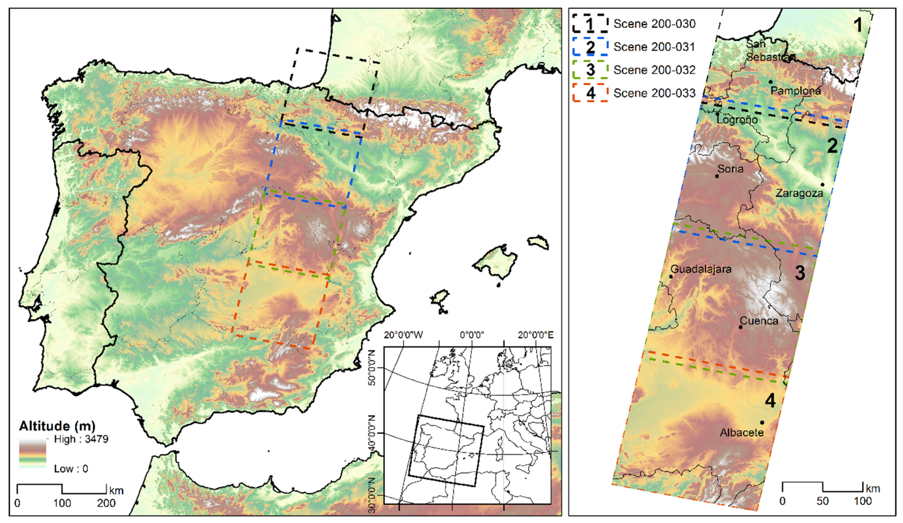
Figure 1. The spatial location of the Landsat scenes in the context of the Iberian Peninsula.
Remotesensing 13 02662 g001
Figure 2. Methodology flowchart. Image pre-processing (A) provided the final variables used in the classification process and NDVI series to characterise the spectral-temporal signatures of the different classes. (B) Structured Query Language (SQL) statements applied to SIOSE 2005 rDS provided a set of polygon selectors which determined the initial GT candidate pixels. (C) The rules applied to GT candidate pixels provided a final set of robust GT samples, segregated into training and test area (TTA) subsets.
Remotesensing 13 02662 g002
Figure 3. The temporal relative frequency distribution of the NDVI is displayed for (a) irrigated herbaceous crops and (b) broadleaf evergreen forest categories. Percentage values are shown in the vertical axis, while the NDVI range of values is presented in the horizontal axis. The red and blue vertical lines define modes (Mo) and antimodes (AMo), respectively; modelled locations are useful when multimodality is assessed [96]. Dates are in year-month-day format.
Remotesensing 13 02662 g003
Figure 4. The NDVI summer multiannual profile of irrigated herbaceous crops is shown. Colour lines in (a) represent the median value of the pixels within polygon tiles. For the sake of simplicity, a random third of the tiles are represented. The red, grey, green and blue dotted lines over date figures denote the imagery (summer months), including 20 July 2005, as a date that is contemporary to the rDS. In (b,c), the polygon is represented in black over two summer dates NDVI (25 July 2001, and 20 July 2005). Note that during the first time period, the pattern is highly stable.
Remotesensing 13 02662 g004
Figure 5. Intra-annual NDVI temporal profile over a coniferous plantation area. Colour lines in (a) represent the median values of the pixels in tile polygons displayed in (b1,b2), and the grey dotted rectangle denotes the intra-annual imagery dates. In (b1,b2), tile polygons are represented with black outlines over 15 August 2000, and 24 September 2000, NDVI.
Remotesensing 13 02662 g005
Figure 6. Composite land cover polygon tiles are shown with a yellow outline. Arrows in (a,b) identify the sparsely vegetated plots.
Remotesensing 13 02662 g006
Figure 7. An example of a mislabelled polygon, depicted in yellow over the orthophotography (a), 28 April 2001 NDVI (b) and 25 July 2001 NDVI (c).
Remotesensing 13 02662 g007
Figure 8. A simple land cover polygon defined as irrigated herbaceous crops is shown in a black tile outline. Multiple phenological behaviours can be identified between spring and summer NDVI responses (ac).
Remotesensing 13 02662 g008
Figure 9. Rule 1 application in a tile polygon. Transitional locations (red squares) with anomalous NDVImax values were selected (green colour) in the left selection (a) but unselected in the right (b). Establishing additional NDVI thresholds (detailed in rule 2) makes it possible to better control the transitional values in composite land cover polygons.
Remotesensing 13 02662 g009
Figure 10. Rule 1 filtering applied over a polygon association.
Remotesensing 13 02662 g010
Figure 11. Rule 1 and 2 applied to a tile polygon. Transitional locations (red squares) in (a,b) with anomalous NDVImax values are correctly selected using Rule 2 restrictions.
Remotesensing 13 02662 g011
Figure 12. Rules 1 and 2 applied over a composite land cover polygon.
Remotesensing 13 02662 g012
Figure 13. Rule 3 applied to irrigated olive grove polygons. Brown NDVI colours depict more recent plantations or low-density plantation schemes. The red square zoom details new plantation fields. The white line in the zoom is a road.
Remotesensing 13 02662 g013
Figure 14. Rule 4 applied to irrigated herbaceous crop polygons. Brown NDVI depict negative NDVI temporal gradients; yellow is related to low contrasting patterns (fallows); green depicts positive NDVI temporal gradients. Positive and negative gradient domains are detailed in zooms 1 and 2.
Remotesensing 13 02662 g014
Figure 15. Rule 5 applied to irrigated herbaceous crops and vineyard crop polygons. Coloured lines depict the pixels selected as NDVI median values in polygons for (a) double crop filtered samples, and (b) dry vineyard woody crop field filtered samples.
Remotesensing 13 02662 g015
Figure 16. Examples of applying the filtering rules. In (A), coniferous polygons affected by clear-cutting forestry practices are shown (outlined in black). An intra-annual NDVI drop is produced. Unfiltered TTA misclassified the area as coniferous forest, while filtered TTA classified the area correctly as shrublands and grasslands. In (B), a mislabelled broadleaf evergreen forest (in white) polygon and a correctly labelled broadleaf polygon.
Remotesensing 13 02662 g016
Figure 17. Examples of the application of filtering rules. In (C), irrigated and dry herbaceous crop patterns coexist within irrigated herbaceous crop polygons (outlined in black). Unfiltered TTA misclassified dry patterns as irrigated crops, while filtered TTA correctly discriminated between categories. In (D), an irregular, high NDVI activity is located in dry vineyard woody crop polygons (in black). Unfiltered TTA misclassified the crop fields as dry woody crops, while the filtered TTA correctly classified them as irrigated woody crops.
Remotesensing 13 02662 g017
Figure 18. Comparison of the omission (a) error (OE) and commission (b) error (CE) regarding unfiltered (uf.) and filtered (f.) ground truth areas. Figures refer to SIOSE 2005 and LCM-2002 imagery.
Remotesensing 13 02662 g018
Table 1. Land cover composition and spatial distribution labelling within SIOSE polygons.
Land Cover CompositionSIOSE_CODE Database FieldVisual Example
SimpleCHLsc 1 Remotesensing 13 02662 i001
Composite in Regular MosaicR(55FDP_45CHLsc) 2 Remotesensing 13 02662 i002
Composite in Irregular MosaicI(50CHLsc_35FDP_15PST) 2 Remotesensing 13 02662 i003
Composite in AssociationA(40CNF_40PST_20MTR) 2 Remotesensing 13 02662 i004
A figure to define the percentage occupation is not required in 1 simple land cover polygons since the land cover occupies 100% of the total area. Any form of 2 composite land cover polygons is characterised by a mixture of land covers (potentially different phenological responses), which could derive into error-prone GT areas.
Table 2. Confusion matrix results derived from unfiltered ground truth samples from SIOSE 2005 rDS and imagery for LCM-2002.
Classified MapUnfiltered Ground Truth SamplesTotalCE (%)UA (%)
CoFBDFBEFShlGrlBrSUrbWaBIHCDHCIWCDWCRiC
(CoF) Coniferous forest50,9078231058161229534312511551529154,8957.392.7
(BDF) Broadleaf deciduous forest104467,72814031884107791011163173590073,6348.092.0
(BEF) Broadleaf evergreen forest5640164460,658739878510952641197527076,53420.779.3
(Shl) Shrublands371515873007115,6889356938160105301245018021547139,64917.282.8
(Grl) Grasslands50467842913,54486,142113539188248148224125211112,94823.776.3
(BrS) Bare soils645452488121435457805862523670626843.456.6
(Urb) Urban areas and Infrastructures1306653572802748300571121350720.179.9
(WaB) Water bodies11005920148812204015433.596.5
(IHC) Irrigated herbaceous crops1718434248681551451337,1145524152682530447,10021.278.8
(DHC) Dry herbaceous crops55514316471853636293826709175,596984276417190,7297.992.1
(IWC) Irrigated woody crops2614612274231101226122154921984140112717,98245.354.7
(DWC) Dry woody crops9911221614545124368269672748309829,2321238,86624.875.2
(RiC) Rice crops51102012164667341021494226734.165.9
NoData3112051841111490000000547
Total62,11073,04966,739144,748102,55270774153181749,057196,79316,02140,4791875766,469OA = 83.8%
OE (%)18.07.39.120.116.049.932.518.124.310.838.627.820.3 OAw = 88.6%
PA (%)82.092.790.979.984.050.167.581.975.789.261.472.279.7 k = 0.7
OE: omission error, CE: commission error, PA: producer’s accuracy, UA: user’s accuracy, k: kappa index of agreement, OA: overall accuracy, OAw: overall accuracy weighted by the ground truth area considering only classified pixels (unclassified pixels are not considered errors and are solved by spatial proximity). Figures in bold represent positions where the predicted label is equal to the true label.
Table 3. Confusion matrix results derived from filtered ground truth samples from SIOSE 2005 rDS and imagery for LCM-2002.
Classified MapFiltered Ground Truth SamplesTotalCE (%)UA (%)
CoFBDFBEFShlGrlBrSUrbWaBIHCDHCIWCDWCRiC
(CoF) Coniferous forest46,9592265253112220003440048,2542.797.3
(BDF) Broadleaf deciduous forest38883,49933055906000940330085,3062.197.9
(BEF) Broadleaf evergreen forest489193452,7183278300000717130062,15715.284.8
(Shl) Shrublands16343111889115,2916468973901541033711780127,6709.790.3
(Grl) Grasslands4834218428184,01232130663616141481093,92410.689.4
(BrS) Bare soils000163310,379494001711060012,69218.281.8
(Urb) Urban areas and Infrastructures00041795678002201133061177.292.8
(WaB) Water bodies000000015780000015780.0100.0
(IHC) Irrigated herbaceous crops28401513400027,6761815070528,6033.296.8
(DHC) Dry herbaceous crops00057624874759023189,4971313440193,1911.998.1
(IWC) Irrigated woody crops16277182322960180164018325,47490028,2449.890.2
(DWC) Dry woody crops1001422120833300952669668,756077,09010.889.2
(RiC) Rice crops00000000201000958115917.382.7
NoData00000000000000
Total53,93985,67255,499124,96394,20411,7947002157829,735201,10526,49273,042963765,986OA = 93.0%
OE (%)12.92.55.07.710.812.018.90.06.95.83.85.90.5 OAw = 95.9%
PA (%)87.197.595.092.389.288.081.1100.093.194.296.294.199.5 k = 0.9
OE: omission error, CE: commission error, PA: producer’s accuracy, UA: user’s accuracy, k: kappa index of agreement, OA: overall accuracy, OAw: overall accuracy weighted by the ground truth area considering only classified pixels (unclassified pixels are not considered errors and are solved by spatial proximity). Figures in bold represent positions where the predicted label is equal to the true label.
Table 4. Summary statistics of the confusion matrices considering unfiltered and filtered GT samples derived from SIOSE 2005 and 2011 in three temporal cases and one spatial case.
LCM-1987 LCM-2012LCM-2017LCM-2002 *
OE (%)CE (%)OE (%)CE (%)OE (%)CE (%)OE (%)CE (%)
uf.f.uf.f.uf.f.uf.f.uf.f.uf.f.uf.f.uf.f.
CoF22.916.818.88.712.010.05.32.117.911.511.13.513.57.415.26.1
BDF25.03.821.22.85.22.67.11.421.12.614.23.322.26.926.115.3
BEF10.35.825.516.07.53.315.713.59.83.319.913.415.36.618.311.6
Shl36.65.420.79.317.44.717.75.941.56.025.16.249.230.633.116.7
Grl26.312.923.511.216.27.120.58.819.69.224.512.115.48.516.99.8
BrS45.19.340.312.247.513.932.418.551.26.341.922.249.219.541.919.9
Urb56.010.415.319.419.612.310.46.027.18.615.226.746.438.230.514.2
WaB21.80.03.30.03.90.22.50.05.30.04.10.013.706.40
IHC31.57.323.76.419.02.623.84.929.22.932.16.317.50.720.81.3
DHC16.46.811.21.411.15.16.81.315.05.18.81.49.56.94.21.6
IWC37.77.450.613.534.812.240.46.542.014.948.95.940.22.660.43.4
DWC15.24.828.210.734.54.625.116.020.217.828.315.412.82.615.612.6
RiC66.70.059.80.018.85.017.81.613.47.143.517.6--------
OA77.592.5 85.694.2 78.793.4 85.192.3
K0.70.9 0.80.9 0.70.9 0.80.9
OA = Overall accuracy, OE = omission error, PA = producer accuracy, CE = commission error, UA = user accuracy, K = Kappa statistic, uf. = unfiltered GT samples, f. = filtered GT samples. LCM-2002 * refers to spatial test assessed in the southern scenes (200-032 and 200-033).
Publisher’s Note: MDPI stays neutral with regard to jurisdictional claims in published maps and institutional affiliations.