
Continuous Sensing of Water Temperature in a Reservoir with Grid Inversion Method Based on Acoustic Tomography System


Abstract
:1. Introduction
2. Methods
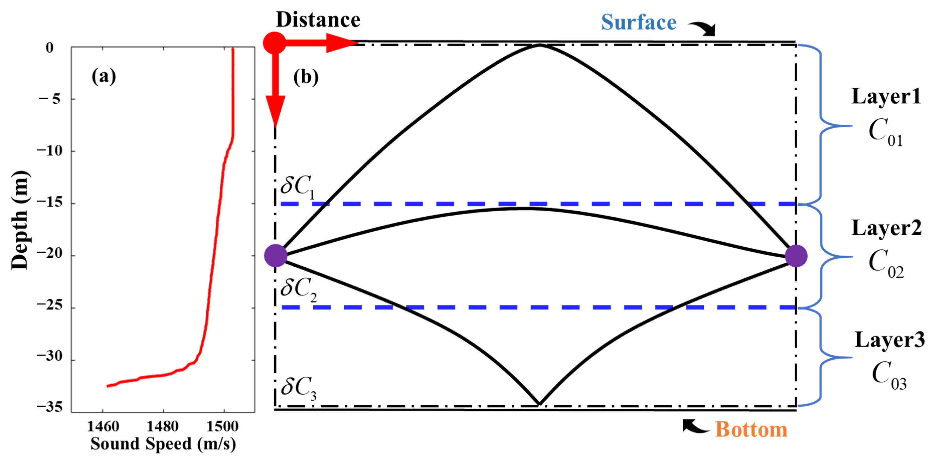
2.1. Layer-Averaged Inversion (Layer Method)
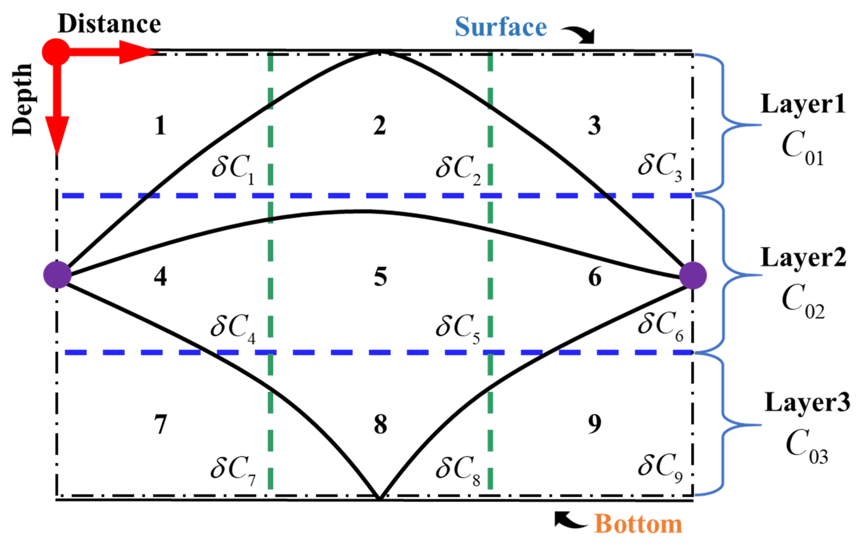
2.2. Two-Dimensional Vertical Water Temperature Field Reconstruction (Grid Method)
3. Experiment and Ray Tracing
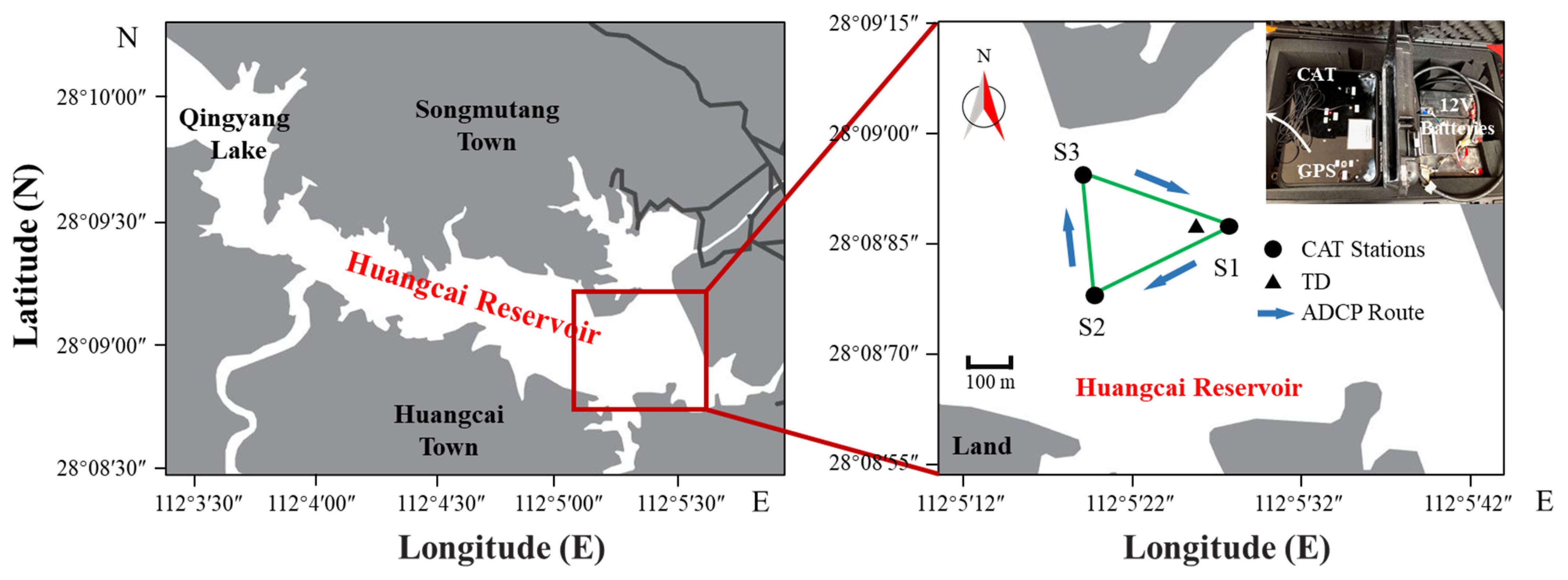
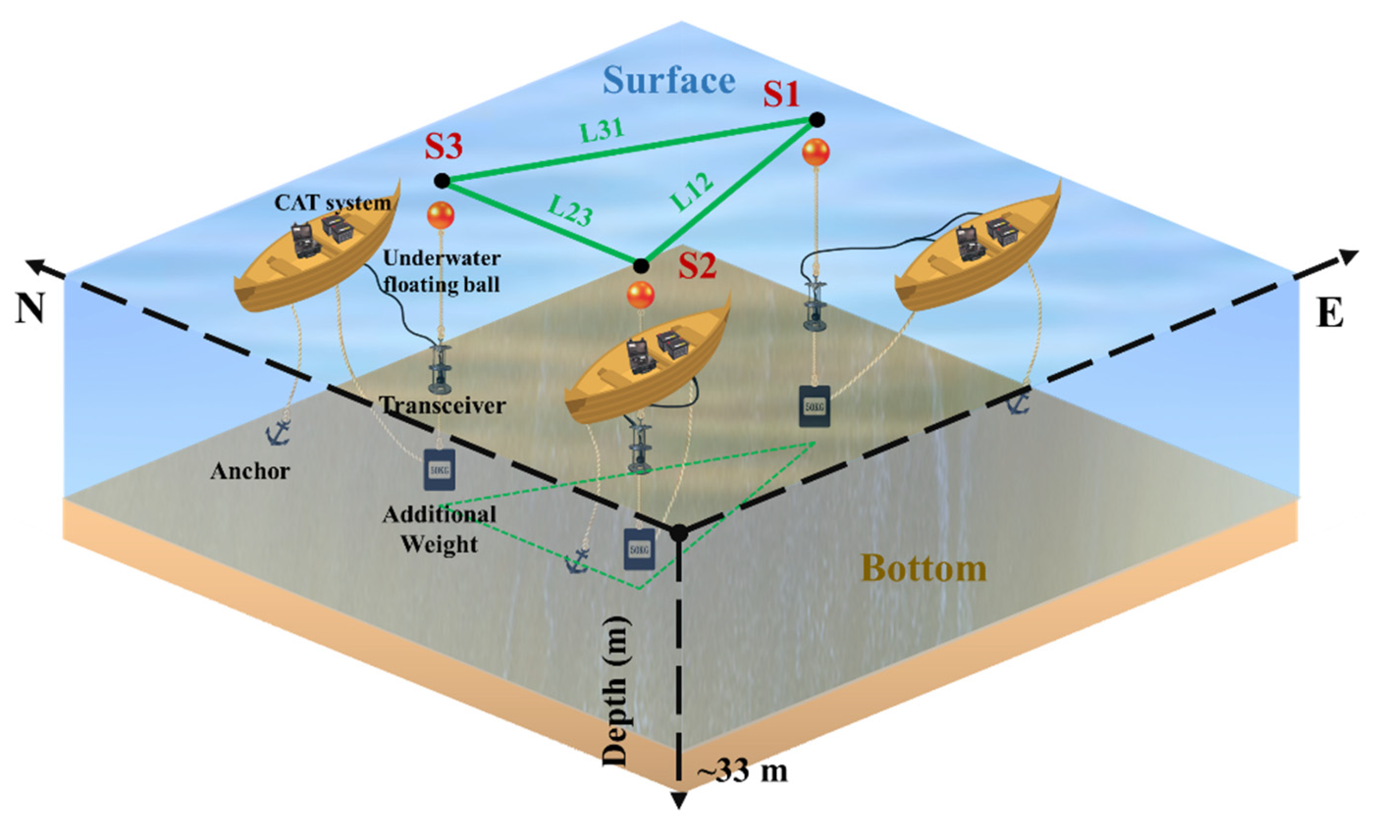
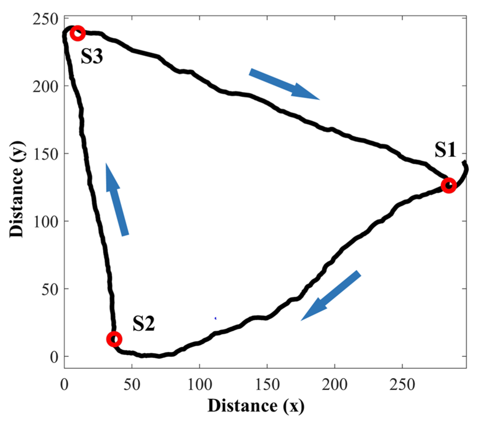
3.1. Experimental Settings
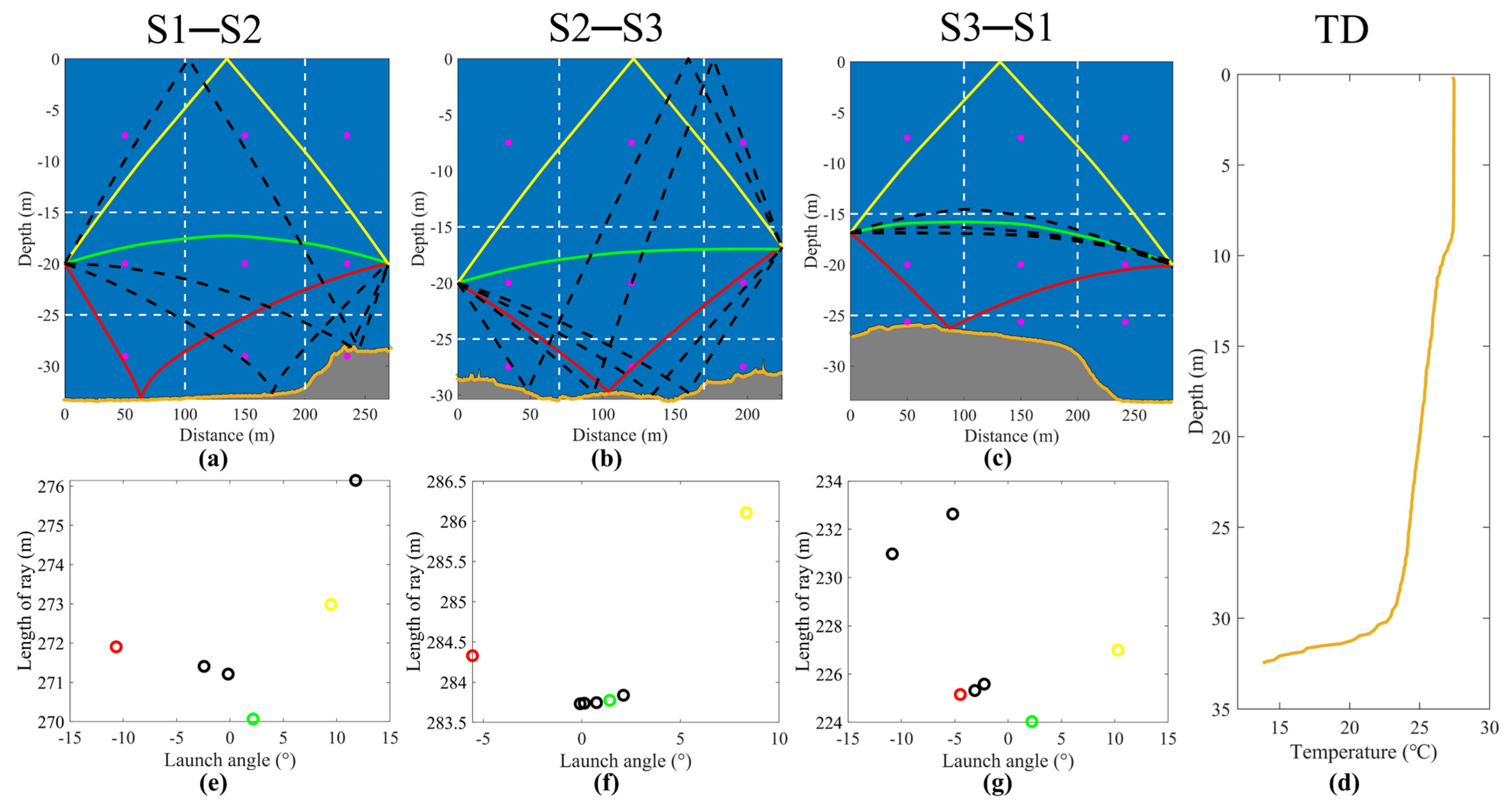
3.2. Ray Tracing
4. Signal Processing and Results
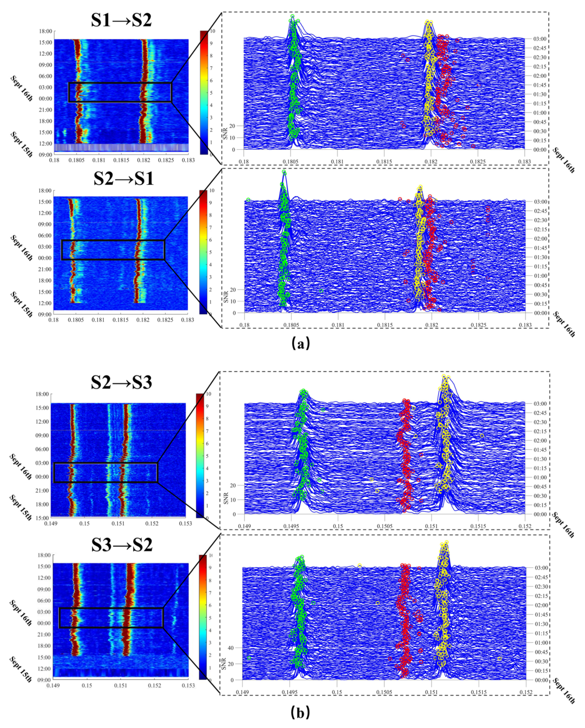
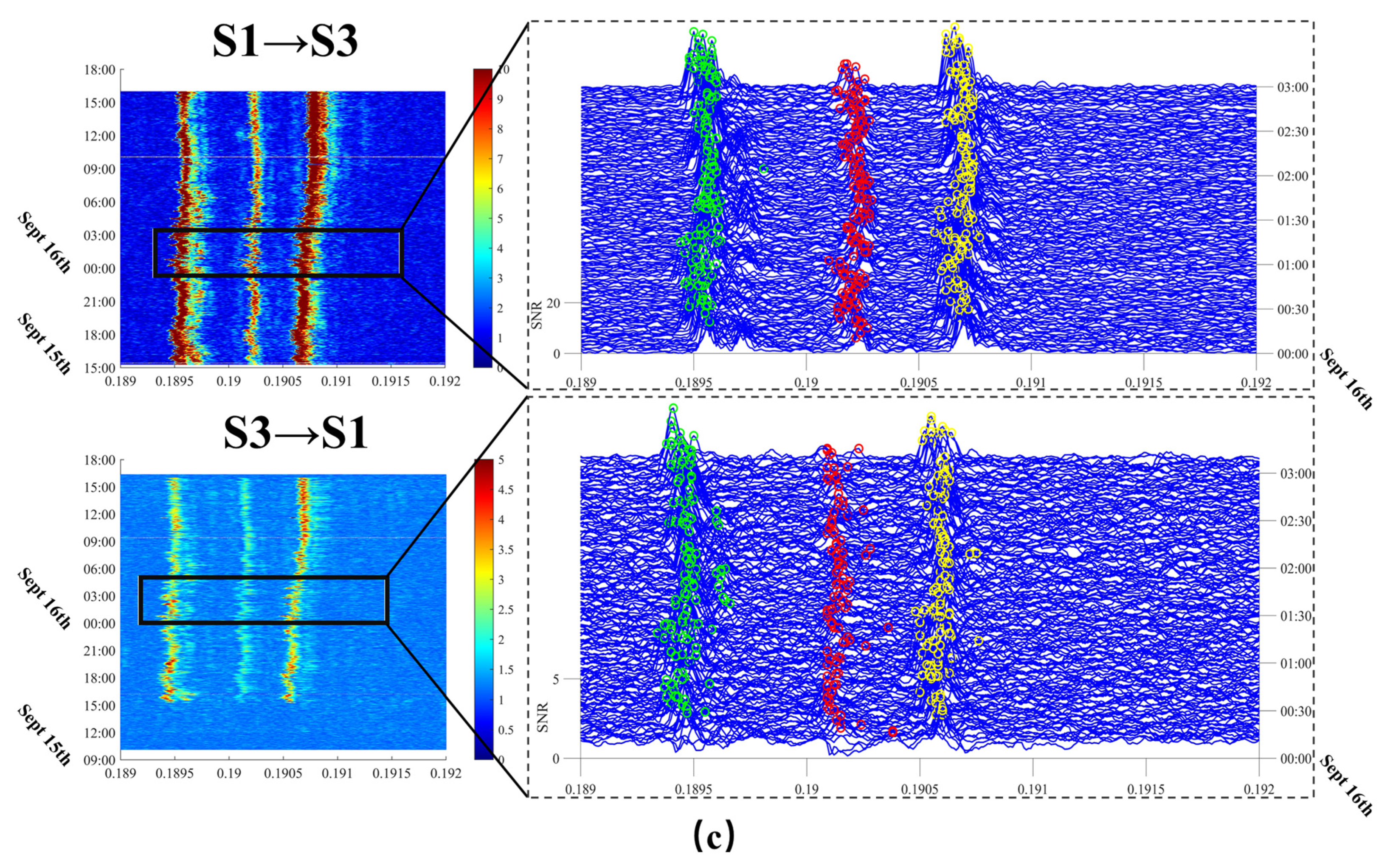
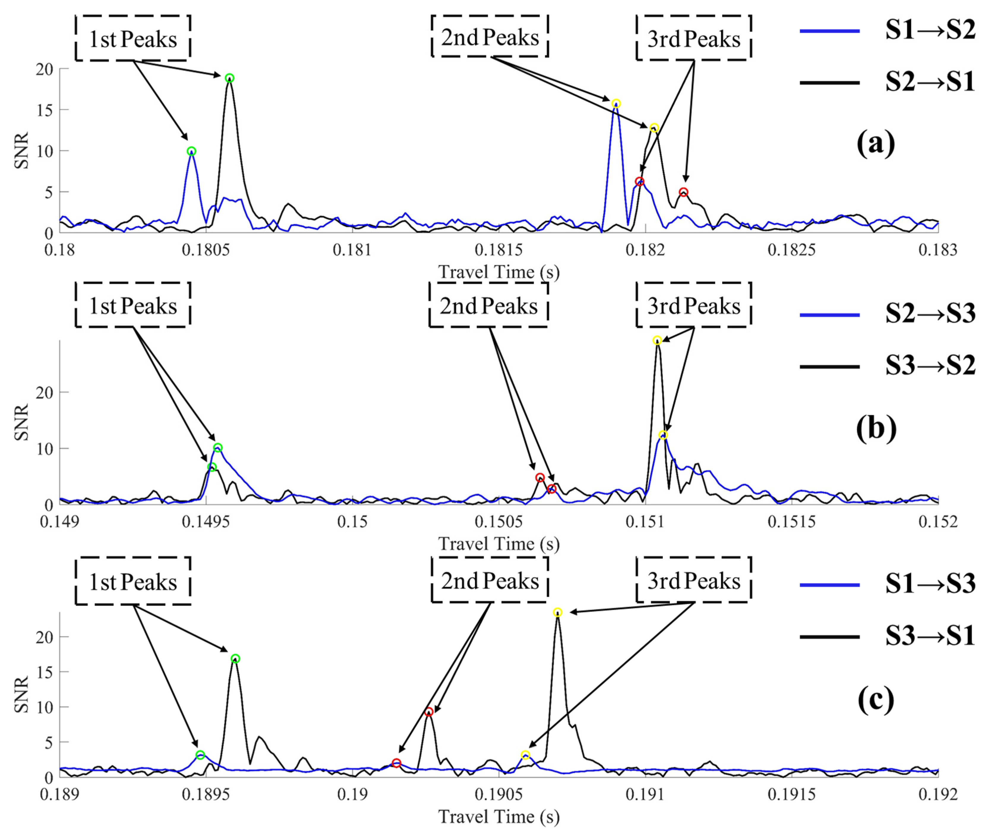
4.1. Multi-Peak Identification
4.2. Inverted Water Temperature Profiling
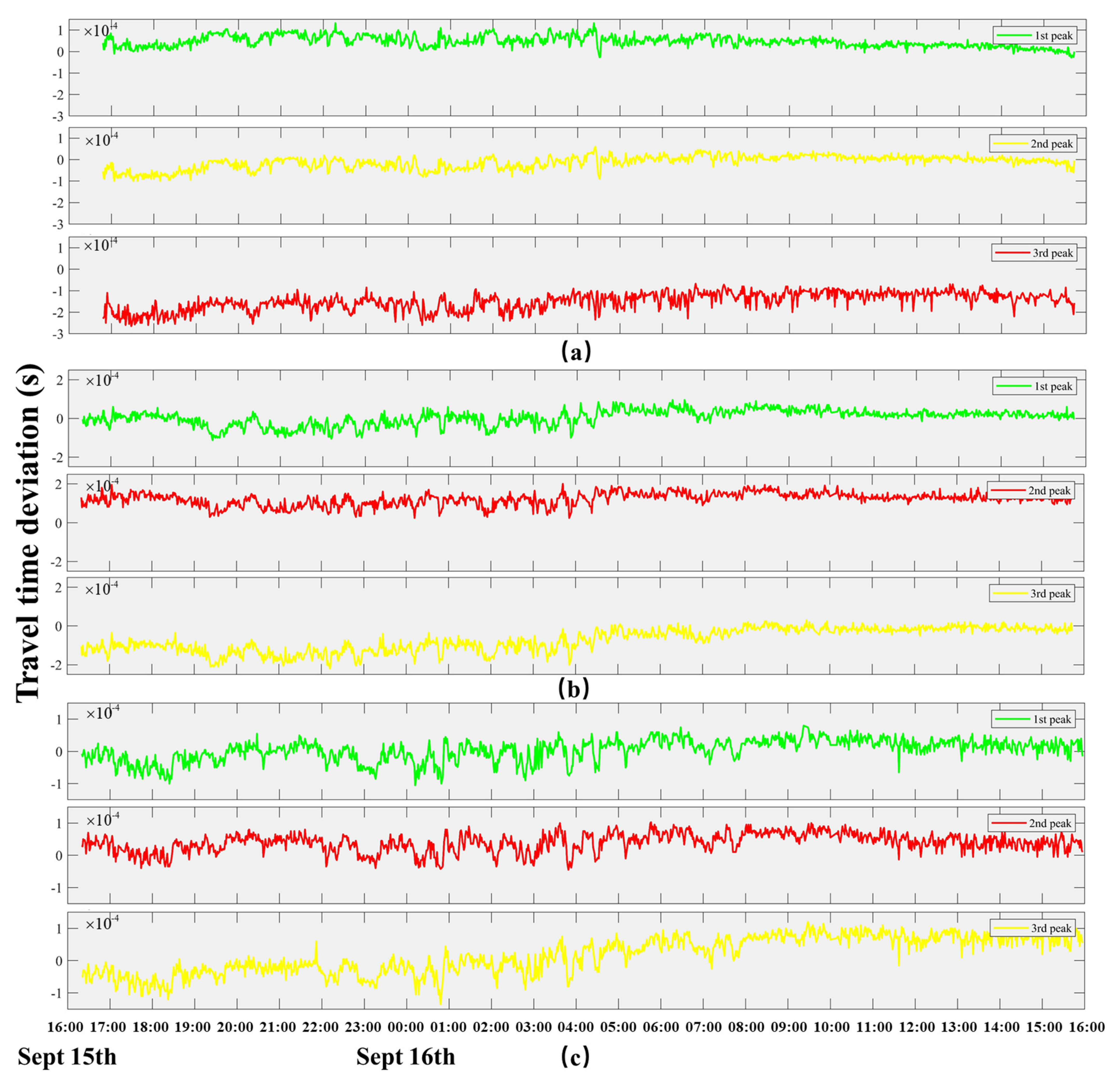
4.2.1. Travel Time Deviation Preprocessing
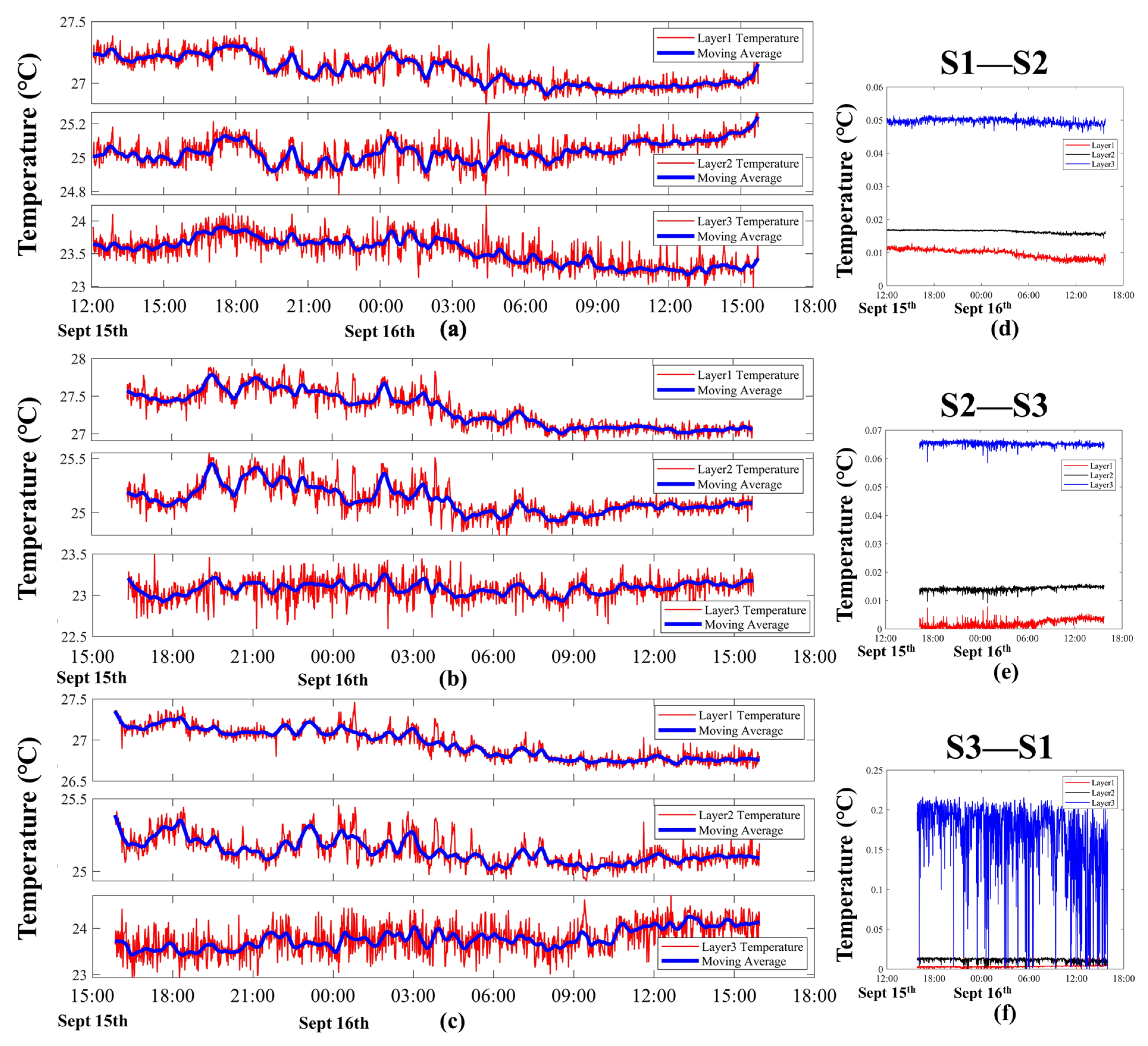
4.2.2. Layer-Averaged Water Temperature
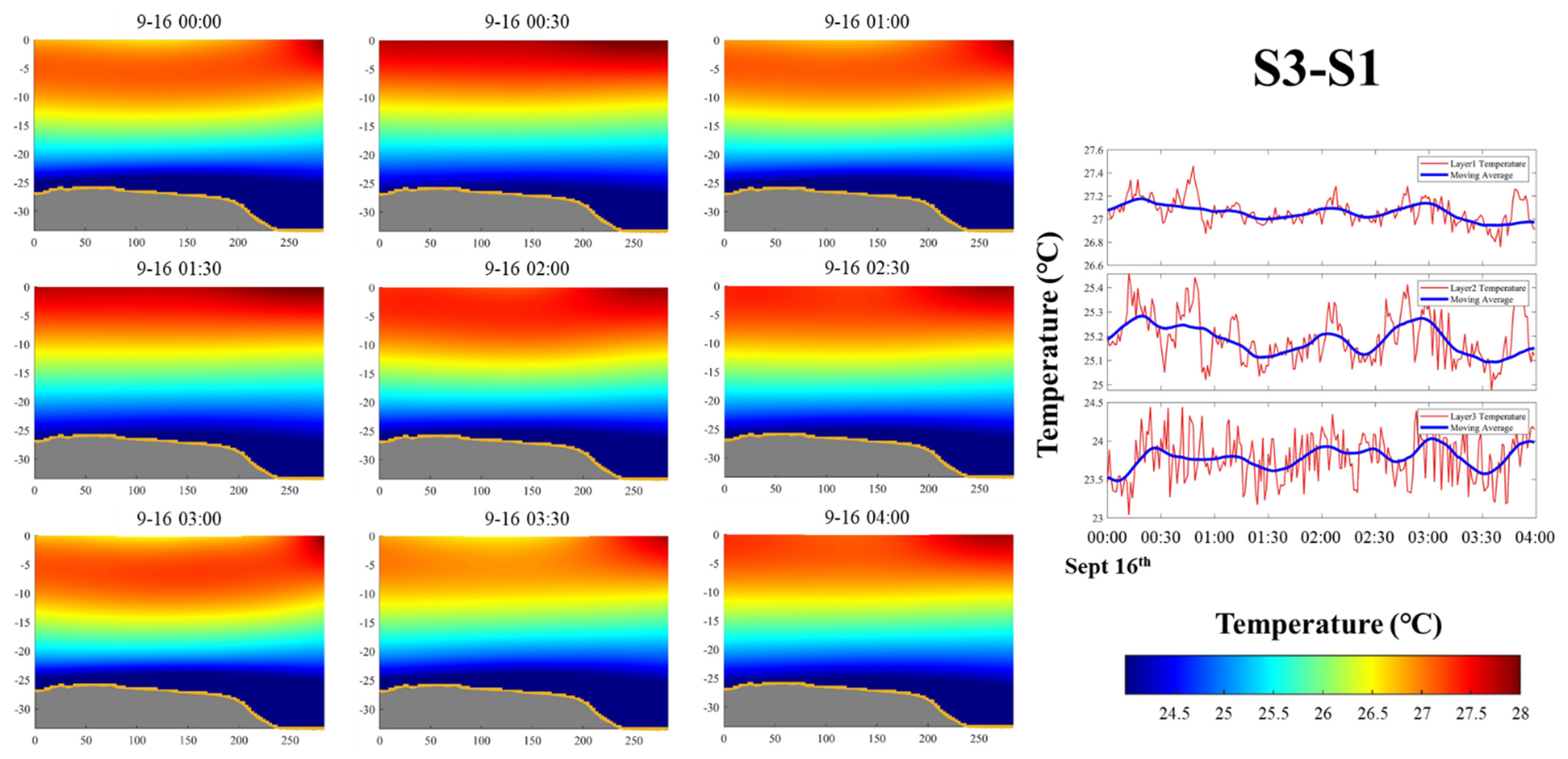
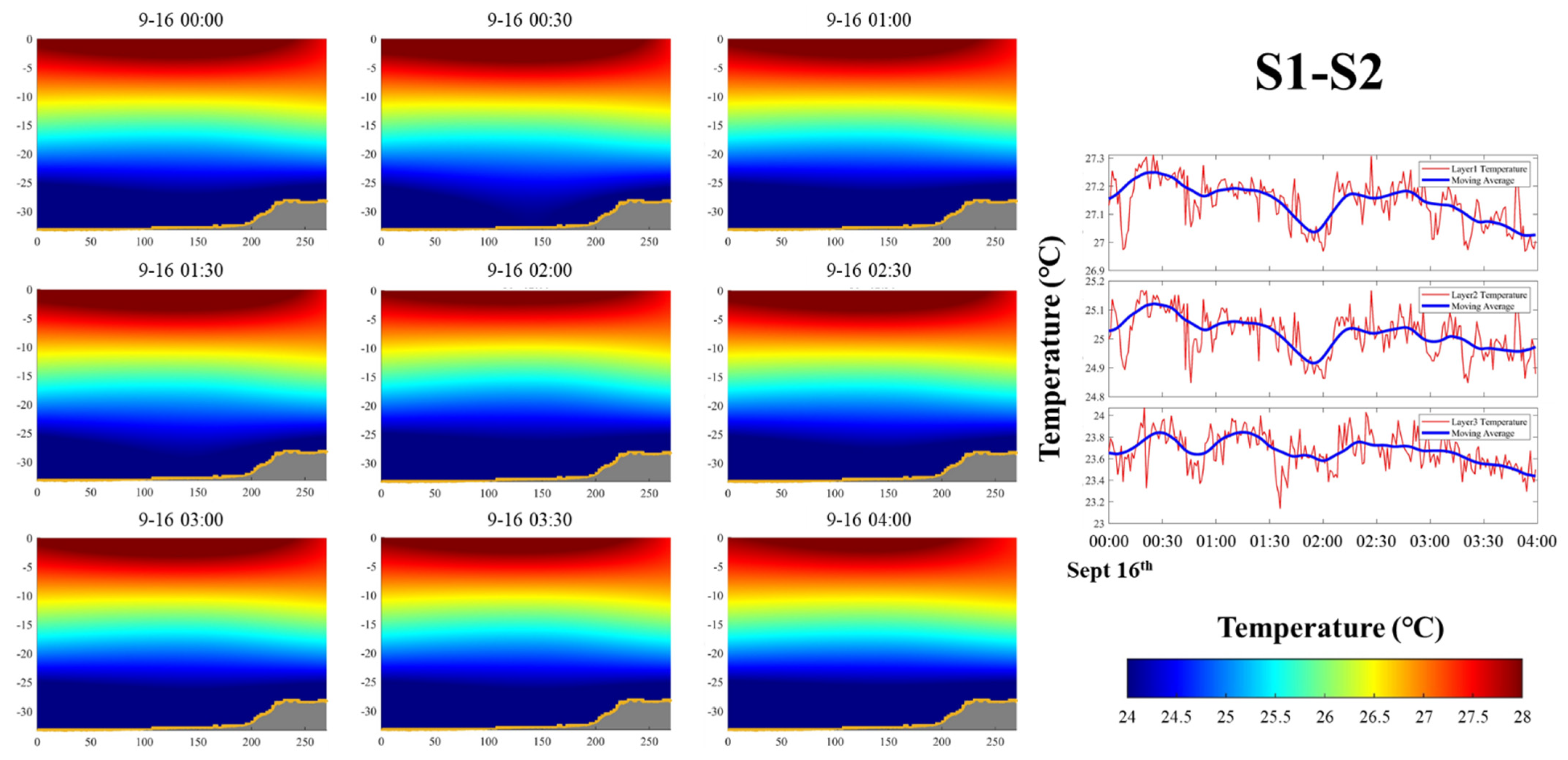
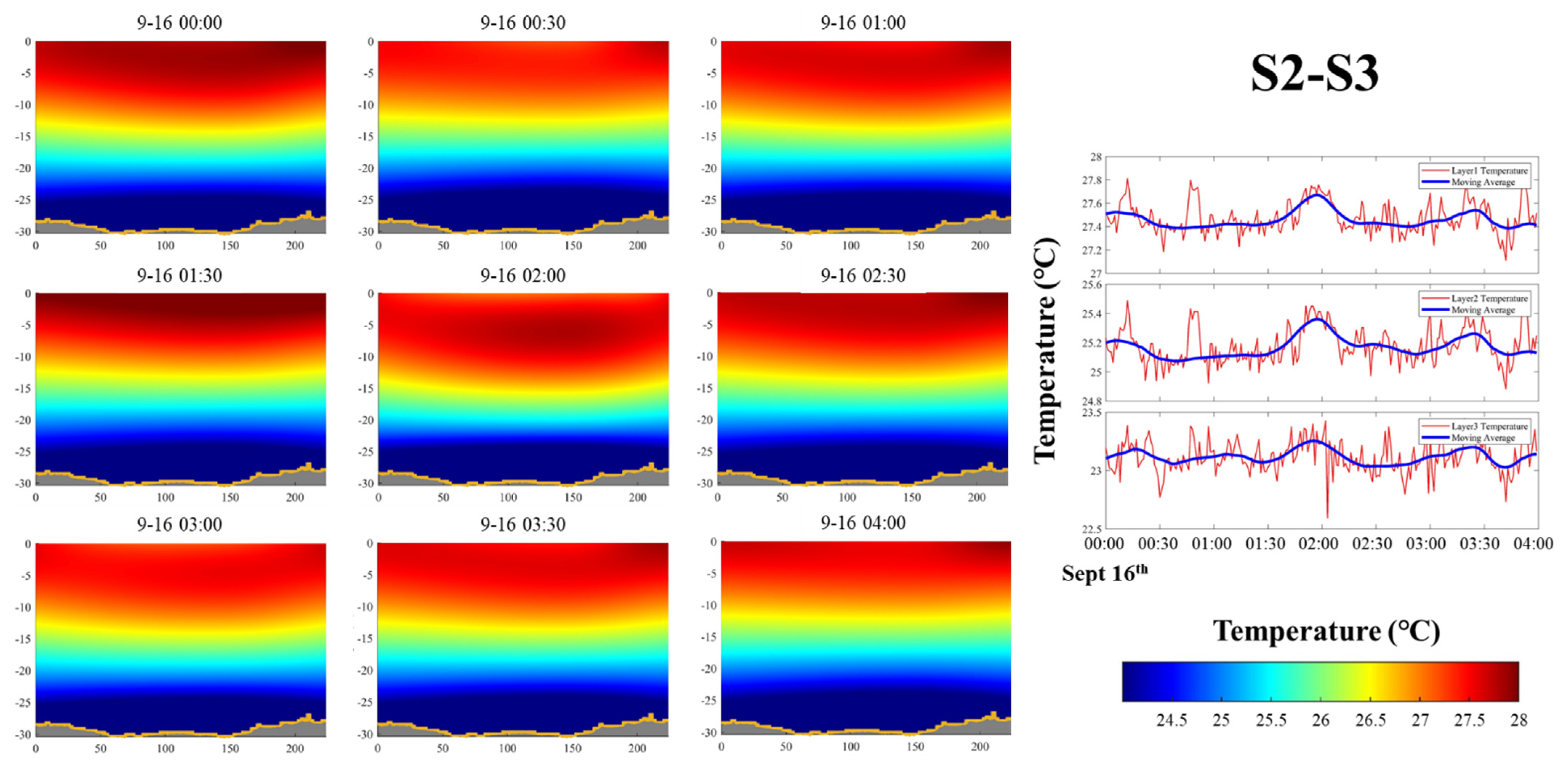
4.2.3. Two-Dimensional Grid Inversion Method
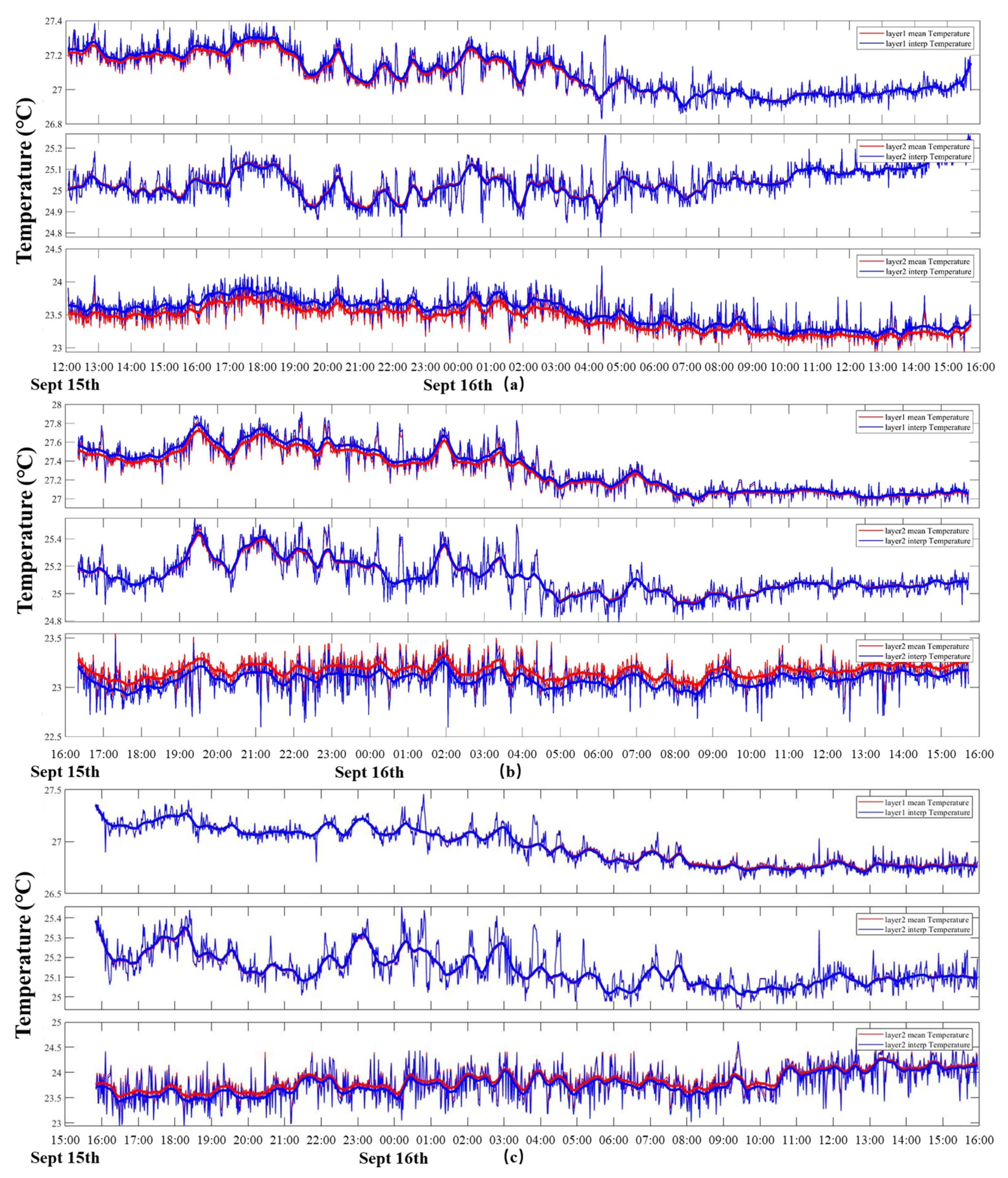
4.3. Comparison of Inversion Results
5. Conclusions
- The quality of the 2D vertical water temperature field is highly dependent on the number of sound rays that are identified. Although obvious multi-arrival ray paths can be identified from the cross-correlation of received acoustic data, it is difficult to match the ray simulation results with the real multi-arrival signal peaks. Consequently, two important factors of high-quality data are: (1) adequate arrival peaks of cross-correlation data, and (2) accurate topographic data of the experimental areas.
- A two-dimensional vertical water temperature field can be successfully established by the grid method with sound waves. The 2D vertical water temperature field is more intuitive than the layer-averaged results in displaying the distributions and trends of different positions during the observation period.
- By error analysis and comparison with the layer-averaged method, the method proposed in this paper is proved to be of high accuracy to profile the vertical temperature field along a vertical slice.
Author Contributions
Funding
Institutional Review Board Statement
Informed Consent Statement
Data Availability Statement
Acknowledgments
Conflicts of Interest
References
- Kaneko, A.; Zhu, X.; Lin, J. Coastal Acoustic Tomography; Academic Press: Cambridge, MA, USA; Elsevier: Amsterdam, The Netherlands, 2020. [Google Scholar]
- Anas, A.; Krishna, K.; Vijayakumar, S.; George, G.; Menon, N.; Kulk, G.; Chekidhenkuzhiyil, J.; Ciambelli, A.; Kuttiyilmemuriyil Vikraman, H.; Tharakan, B.; et al. Dynamics of Vibrio cholerae in a Typical Tropical Lake and Estuarine System: Potential of Remote Sensing for Risk Mapping. Remote Sens. 2021, 13, 1034. [Google Scholar] [CrossRef]
- Hidalgo Garcia, D.; Arco Diaz, J. Spatial and Multi-Temporal Analysis of Land Surface Temperature through Landsat 8 Images: Comparison of Algorithms in a Highly Polluted City (Granada). Remote Sens. 2021, 13, 1012. [Google Scholar] [CrossRef]
- Syamsudin, F.; Chen, M.; Kaneko, A.; Adityawarman, Y.; Zheng, H.; Mutsuda, H.; Hanifa, A.D.; Zhang, C.; Auger, G.; Wells, J.C.; et al. Profiling measurement of internal tides in Bali Strait by reciprocal sound transmission. Acoust. Sci. Technol. 2017, 38, 246–253. [Google Scholar] [CrossRef]
- Wang, L.; Wang, Y.; Wang, J.; Li, F. A High Spatial Resolution FBG Sensor Array for Measuring Ocean Temperature and Depth. Photonic Sens. 2020, 10, 57–66. [Google Scholar] [CrossRef] [Green Version]
- Munk, W.; Wunsch, C. Ocean acoustic tomography—Scheme for large-scale monitoring. Deep Sea Res. Part A Oceanogr. Res. Pap. 1979, 26, 123–161. [Google Scholar] [CrossRef]
- Munk, W.; Worceser, P.F.; Wunsch, C. Ocean Acoustic Tomography; Cambridge Univ. Press: New York, NY, USA, 1995; p. 433. [Google Scholar]
- Duda, T.F.; Flatte, S.M.; Colosi, J.A.; Cornuelle, B.D.; Hildebrand, J.A.; Hodgkiss, W.S.; Worcester, P.F.; Howe, B.M.; Mercer, J.A.; Spindel, R.C. Measured wave-front fluctuations in 1000-km pulse-propagation in the pacific-ocean. J. Acoust. Soc. Am. 1992, 92, 939–955. [Google Scholar] [CrossRef]
- Skarsoulis, E.K.; Athanassoulis, G.A.; Send, U. Ocean acoustic tomography based on peak arrivals. J. Acoust. Soc. Am. 1996, 100, 797–813. [Google Scholar] [CrossRef]
- Hong, Z.; Haruhiko, Y.; Noriaki, G.; Hideaki, N.; Arata, K. Design of the acoustic tomography system for velocity measurement with an application to the coastal sea. Acoust. Soc. Jpn. 1998, 19, 199–210. [Google Scholar]
- Zhang, C.; Kaneko, A.; Zhu, X.-H.; Gohda, N. Tomographic mapping of a coastal upwelling and the associated diurnal internal tides in Hiroshima Bay, Japan. J. Geophys. Res. Ocean. 2015, 120, 4288–4305. [Google Scholar] [CrossRef]
- Zhang, C.; Kaneko, A.; Zhu, X.-H.; Howe, B.M.; Gohda, N. Acoustic measurement of the net transport through the Seto Inland Sea. Acoust. Sci. Technol. 2016, 37, 10–20. [Google Scholar] [CrossRef]
- Huang, H.; Guo, Y.; Wang, Z.; Shen, Y.; Wei, Y. Water Temperature Observation by Coastal Acoustic Tomography in Artificial Upwelling Area. Sensors 2019, 19, 2655. [Google Scholar] [CrossRef] [Green Version]
- Huang, H.; Guo, Y.; Li, G.; Arata, K.; Xie, X.; Xu, P. Short-Range Water Temperature Profiling in a Lake with Coastal Acoustic Tomography. Sensors 2020, 20, 4498. [Google Scholar] [CrossRef]
- Roux, P.; Cornuelle, B.D.; Kuperman, W.A.; Hodgkiss, W.S. The structure of raylike arrivals in a shallow-water waveguide. J. Acoust. Soc. Am. 2008, 124, 3430–3439. [Google Scholar] [CrossRef]
- Elisseeff, P.; Schmidt, H.; Johnson, M.; Herold, D.; Chapman, N.R.; McDonald, M.M. Acoustic tomography of a coastal front in Haro Strait, British Columbia. J. Acoust. Soc. Am. 1999, 106, 169–184. [Google Scholar] [CrossRef]
- Luo, J.; Karjadi, E.A.; Badiey, M. High-frequency broadband acoustic current tomography in shallow water. J. Acoust. Soc. Am. 2008, 123, 3914. [Google Scholar] [CrossRef]
- Li, G.; Ingram, D.; Kaneko, A.; Chen, M.; Gohda, N.; Polydorides, N. Vertical underwater acoustic tomography in an experimental basin. J. Acoust. Soc. Am. 2017, 141, 3656. [Google Scholar] [CrossRef]
- Yu, X.; Zhuang, X.; Li, Y.; Zhang, Y. Real-Time Observation of Range-Averaged Temperature by High-Frequency Underwater Acoustic Thermometry. IEEE Access 2019, 7, 17975–17980. [Google Scholar] [CrossRef]
- Huang, C.-F.; Chen, K.; Huang, S.-W.; Guo, J.; Taniguchi, N. Acoustic mapping of ocean currents using moving vehicles. J. Acoust. Soc. Am. 2018, 144, 1982. [Google Scholar] [CrossRef]
- Huang, C.-F.; Li, Y.-W.; Taniguchi, N. Mapping of ocean currents in shallow water using moving ship acoustic tomography. J. Acoust. Soc. Am. 2019, 145, 858–868. [Google Scholar] [CrossRef] [PubMed]
- Chen, K.; Huang, C.-F.; Huang, S.-W.; Liu, J.-Y.; Guo, J. Mapping coastal circulations using moving vehicle acoustic tomography. J. Acoust. Soc. Am. 2020, 148, EL353–EL358. [Google Scholar] [CrossRef]
- Carriere, O.; Hermand, J.-P. Feature-Oriented Acoustic Tomography for Coastal Ocean Observatories. IEEE J. Ocean. Eng. 2013, 38, 534–546. [Google Scholar] [CrossRef]
- Syamsudin, F.; Taniguchi, N.; Zhang, C.; Hanifa, A.D.; Li, G.; Chen, M.; Mutsuda, H.; Zhu, Z.-N.; Zhu, X.-H.; Nagai, T.; et al. Observing Internal Solitary Waves in the Lombok Strait by Coastal Acoustic Tomography. Geophys. Res. Lett. 2019, 46, 10475–10483. [Google Scholar] [CrossRef] [Green Version]
- Liu, W.; Zhu, X.; Zhu, Z.; Fan, X.; Dong, M.; Zhang, Z. A Coastal Acoustic Tomography Experiment in the Qiongzhou Strait; IEEE: Piscataway, NJ, USA, 2016. [Google Scholar]
- Mackenzie, K.V. Nine-term equation for sound speed in the oceans. J. Acoust. Soc. Am. 1981, 70, 807–812. [Google Scholar] [CrossRef]


| Item | Value | ||
|---|---|---|---|
| Central frequency (kHz) | 50 | ||
| Order of M sequence | 10 | ||
| Q 1 | 2 | ||
| Transmit interval (min) | 1 | ||
| Start and end date | Sept.15 09:00–Sept.16 16:00 | ||
| Station | S1 | S2 | S3 |
| Station distance (m) 2 | L12 = 270.00 | L23 = 224.01 | L31 = 283.64 |
| Transceiver depth (m) | 20 | 20 | 16.86 |
| Stations | S1–S2 | S2–S3 | S3–S1 | ||||||
|---|---|---|---|---|---|---|---|---|---|
| Ray Path | D 1 | S 2 | B 3 | D | S | B | D | S | B |
| Layer 1 | 0 | 209.946 | 0 | 0 | 188.490 | 0 | 0 | 238.576 | 0 |
| Layer 2 | 270.068 4 | 272.983 | 142.737 | 224.037 | 38.509 | 139.634 | 283.775 | 47.533 | 249.815 |
| Layer 3 | 0 | 0 | 129.167 | 0 | 0 | 85.523 | 0 | 0 | 34.515 |
| Total 4 (m) | 270.068 | 272.98 | 271.904 | 224.037 | 226.999 | 225.157 | 283.775 | 286.109 | 284.33 |
| TT 5 (s) | 0.18038 | 0.18191 | 0.18217 | 0.14962 | 0.15124 | 0.15061 | 0.18947 | 0.19061 | 0.19010 |
| Stations | S1–S2 | S2–S3 | S3–S1 | ||||||
|---|---|---|---|---|---|---|---|---|---|
| Ray Path | D | S | B | D | S | B | D | S | B |
| Grid 1 | 0 | 70.033 | 0 | 0 | 42.469 | 0 | 0 | 66.249 | 0 |
| Grid 2 | 0 | 100.97 | 0 | 0 | 101.22 | 0 | 0 | 100.73 | 0 |
| Grid 3 | 0 | 38.944 | 0 | 0 | 44.802 | 0 | 0 | 28.498 | 0 |
| Grid 4 | 100.03 | 31.114 | 26.504 | 70.027 | 28.55 | 58.125 | 100.01 | 34.605 | 59.162 |
| Grid 5 | 100.01 | 0 | 46.182 | 100.01 | 0 | 27.246 | 100.01 | 0 | 45.837 |
| Grid 6 | 70.028 | 31.924 | 70.05 | 54 | 9.958 | 54.262 | 83.755 | 56.027 | 83.712 |
| Grid 7 | 0 | 0 | 75.167 | 0 | 0 | 12.147 | 0 | 0 | 44.367 |
| Grid 8 | 0 | 0 | 54.001 | 0 | 0 | 73.377 | 0 | 0 | 54.252 |
| Grid 9 | 0 | 0 | 0 | 0 | 0 | 0 | 0 | 0 | 0 |
| Total (m) | 270.068 | 272.98 | 271.904 | 224.037 | 226.999 | 225.157 | 283.775 | 286.109 | 284.33 |
| TT (s) | 0.18038 | 0.18191 | 0.18217 | 0.14962 | 0.15124 | 0.15061 | 0.18947 | 0.19061 | 0.19010 |
| Peaks | S1→S2 | S2→S1 | S12-RS 1 | |
| 1st Peak | 0.1804 | 0.1805 | 0.18038 | D |
| 2nd Peak | 0.1819 | 0.1820 | 0.18191 | S |
| 3rd Peak | 0.1820 | 0.2821 | 0.18217 | B |
| Peaks | S2→S3 | S3→S2 | S23-RS | |
| 1st Peak | 0.1495 | 0.1496 | 0.14962 | D |
| 2nd Peak | 0.1506 | 0.1507 | 0.15061 | B |
| 3rd Peak | 0.1510 | 0.1511 | 0.15124 | S |
| Peaks | S1→S3 | S3→S1 | S13-RS | |
| 1st Peak | 0.1895 | 0.1896 | 0.18947 | D |
| 2nd Peak | 0.1902 | 0.1903 | 0.19010 | B |
| 3rd Peak | 0.1906 | 0.1907 | 0.19061 | S |
| Stations | S1–S2 | S2–S3 | S3–S1 | ||||||
|---|---|---|---|---|---|---|---|---|---|
| Peaks | 1st Peak | 2nd Peak | 3rd Peak | 1st Peak | 2nd Peak | 3rd Peak | 1st Peak | 2nd Peak | 3rd Peak |
| Terr-M 1 | 0.0097 | 0.0164 | 0.0496 | 0.0019 | 0.0114 | 0.0652 | 0.0037 | 0.0114 | 0.1677 |
| Terr-S 2 | 0.0013 | 0.0005 | 0.0008 | 0.0013 | 0.0142 | 0.1677 | 0.0031 | 0.0026 | 0.0456 |
| RMSE (°C) 1 | S1–S2 | S2–S3 | S3–S1 |
|---|---|---|---|
| Layer 1 | 0.0122 | 0.0359 | 0.0073 |
| Layer 2 | 0.0042 | 0.0084 | 0.0082 |
| Layer 3 | 0.0963 | 0.0873 | 0.0712 |
Publisher’s Note: MDPI stays neutral with regard to jurisdictional claims in published maps and institutional affiliations. |
© 2021 by the authors. Licensee MDPI, Basel, Switzerland. This article is an open access article distributed under the terms and conditions of the Creative Commons Attribution (CC BY) license (https://creativecommons.org/licenses/by/4.0/).
Share and Cite
Huang, H.; Xu, S.; Xie, X.; Guo, Y.; Meng, L.; Li, G. Continuous Sensing of Water Temperature in a Reservoir with Grid Inversion Method Based on Acoustic Tomography System. Remote Sens. 2021, 13, 2633. https://doi.org/10.3390/rs13132633
Huang H, Xu S, Xie X, Guo Y, Meng L, Li G. Continuous Sensing of Water Temperature in a Reservoir with Grid Inversion Method Based on Acoustic Tomography System. Remote Sensing. 2021; 13(13):2633. https://doi.org/10.3390/rs13132633
Chicago/Turabian StyleHuang, Haocai, Shijie Xu, Xinyi Xie, Yong Guo, Luwen Meng, and Guangming Li. 2021. "Continuous Sensing of Water Temperature in a Reservoir with Grid Inversion Method Based on Acoustic Tomography System" Remote Sensing 13, no. 13: 2633. https://doi.org/10.3390/rs13132633
APA StyleHuang, H., Xu, S., Xie, X., Guo, Y., Meng, L., & Li, G. (2021). Continuous Sensing of Water Temperature in a Reservoir with Grid Inversion Method Based on Acoustic Tomography System. Remote Sensing, 13(13), 2633. https://doi.org/10.3390/rs13132633