Automatic Road Marking Extraction and Vectorization from Vehicle-Borne Laser Scanning Data

Abstract

Automatic driving technology is becoming one of the main areas of development for future intelligent transportation systems. The high-precision map, which is an important supplement of the on-board sensors during shielding or limited observation distance, provides a priori information for high-precision positioning and path planning in automatic driving. The position and semantic information of the road markings, such as absolute coordinates of the solid lines and dashed lines, are the basic components of the high-precision map. In this paper, we study the automatic extraction and vectorization of road markings. Firstly, scan lines are extracted from the vehicle-borne laser point cloud data, and the pavement is extracted from scan lines according to the geometric mutation at the road boundary. On this basis, the pavement point clouds are transformed into raster images with a certain resolution by using the method of inverse distance weighted interpolation. An adaptive threshold segmentation algorithm is used to convert raster images into binary images. Followed by the adaptive threshold segmentation is the Euclidean clustering method, which is used to extract road markings point clouds from the binary image. Solid lines are detected by feature attribute filtering. All of the solid lines and guidelines in the sample data are correctly identified. The deep learning network framework PointNet++ is used for semantic recognition of the remaining road markings, including dashed lines, guidelines and arrows. Finally, the vectorization of the identified solid lines and dashed lines is carried out based on a line segmentation self-growth algorithm. The vectorization of the identified guidelines is carried out according to an alpha shape algorithm. Point cloud data from four experimental areas are used for road marking extraction and identification. The F-scores of the identification of dashed lines, guidelines, straight arrows and right turn arrows are 0.97, 0.66, 0.84 and 1, respectively.

1. Introduction

As a key factor needed for travelling by intelligent vehicles in the future, high-precision maps have been widely researched. They can provide prior information for autonomous positioning of automatic driving vehicles with L3 level and above. The ability of autonomous vehicles to perceive the environment through cameras, laser scanners and other sensors is limited. However, a priori information such as the position of lane lines on high-precision maps can narrow the detection range of targets and reduce the difficulty of perception. Vehicle-borne laser point cloud data are important for building high-precision maps. Efficient and automatic extraction of road markings from point cloud data is of great significance to the establishment of high-precision maps. Reliable identification of lane markings—including dashed lines, solid lines and arrows—is important for autonomous driving and driver assistance systems (ADAS) applications [1].

Researchers first obtained road marking information from optical images through an image recognition method [2,3,4,5,6,7]. However, due to the complex and changeable imaging environment in reality, weather changes, tree shadows, car occlusion and other factors add many difficulties to image processing. At present, it is still difficult to fully achieve automated road marking information extraction or to obtain three-dimensional information of objects directly from two-dimensional images. Yan et al. [8] used dynamic windows to perform median filtering on the intensity of point clouds lying on each scanning line. Then, the edge points of the road marking were determined according to the intensity gradient variation of each scanning line. Finally, fake road marking point clouds were removed from the extracted road marking point clouds according to the characteristics of the road markings. Guan et al. [9] determined intensity segmentation thresholds by using a weighted neighboring difference histogram and then extracted road markings by a two-dimensional multi-scale tensor voting algorithm. Yu et al. [10] directly divided the point clouds into several parts along the vertical direction of the vehicle driving track. The intensity segmentation threshold of each part was calculated by the Otsu method and the road markings were extracted based on the calculated threshold value. Finally, the semantic knowledge was used to classify the road markings that had a larger shape. The smaller road markings were recognized by deep learning and principal component analysis. In [11], the original point clouds were first converted into the intensity image, and then, the road markings were extracted from the intensity image by an adaptive threshold segmentation algorithm. Finally, a neural network was used to classify specific categories of the road markings. However, the number of categories identified was limited. Guan et al. [12] noticed that the further away from the laser scanner, the less dense the road point clouds were. Therefore, they proposed a method of extracting road markings with multi thresholds based on point density. In this method, the point clouds are first converted into intensity feature images by inverse distance weighted interpolation, and then, the intensity threshold under different point densities is calculated according to the Otsu algorithm. Finally, the results are further modified by morphological operation. Yang et al. [13] first extracted the road marking point clouds by separating the points with high intensity value and filtering out the point clouds higher than the ground from initial point clouds. Then, they generated the intensity image by the interpolation method. Finally, the road marking point clouds were extracted from the image by combining semantic knowledge, such as the shape and size of the road markings. In [14], the author designed two network frameworks for dealing with point clouds collected by mobile laser scanning system. One is a U-shaped capsule-based network for extracting road markings from generated intensity images. The other is a hybrid capsule-based network for determining the semantic information of extracted road markings. Nevertheless, the training data that are fed into the capsule-based network are still raster images transformed from point clouds, rather than point clouds themselves.

The majority of studies on road marking extraction fail to implement vectorization based on recognized road markings, while high-precision maps need road markings to be vectorized. The main goal of this paper is to extract and recognize road markings from vehicle-borne laser point clouds. Based on the extraction and recognition of road markings, the vectorization of road markings is implemented in this paper.

2. Methodology

In this paper, the process of extraction and recognition of road markings is divided into four steps: the extraction of pavement point clouds, the extraction of road marking point clouds, the recognition of road markings and the vectorization of road markings. The flowchart is shown in Figure 1.

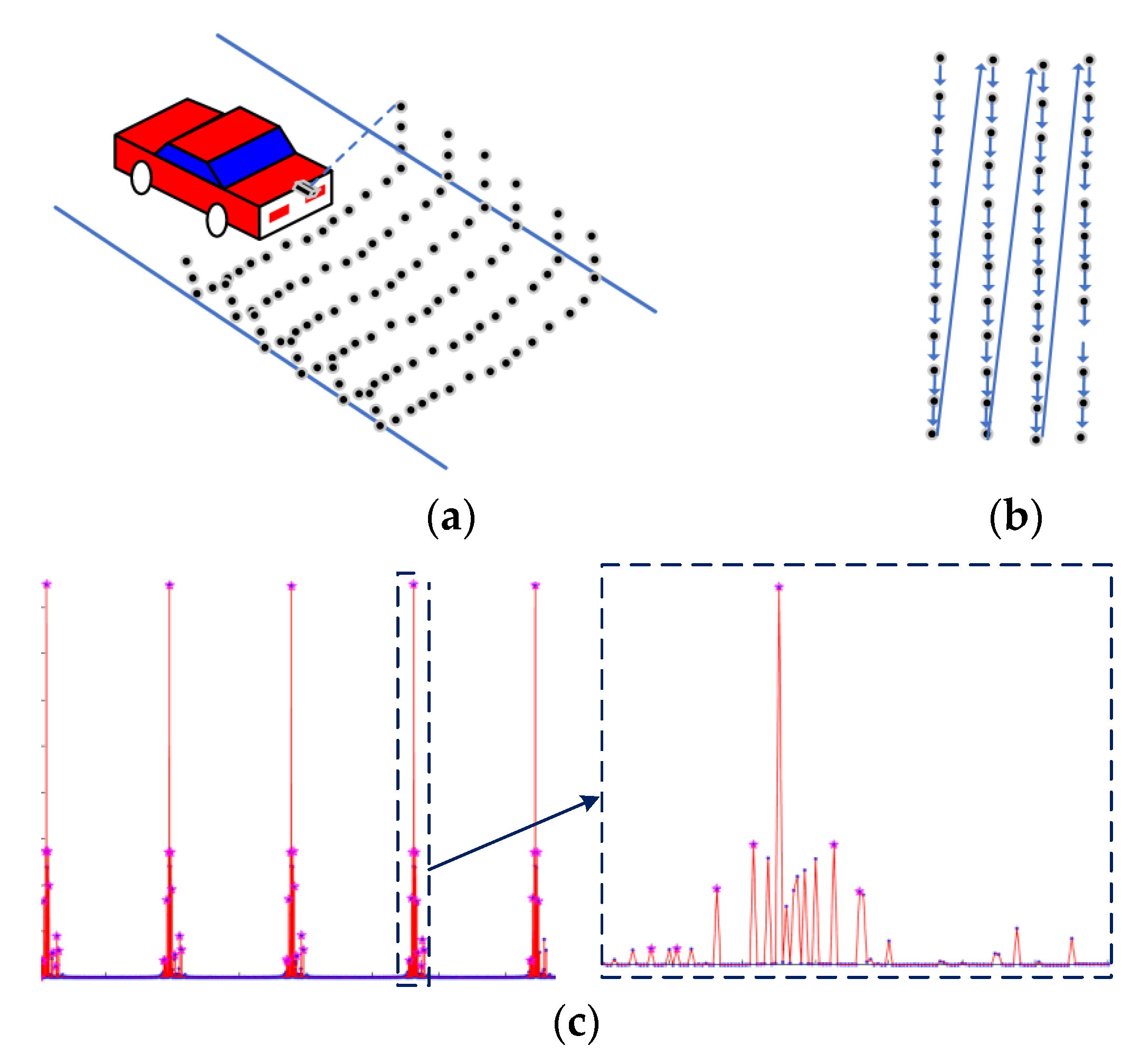
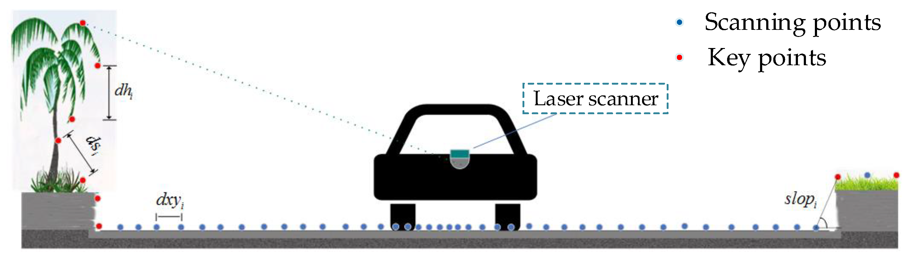
2.1. Pavement Extraction

Since the number of point clouds lying on the scan line is limited and their geometric features are obvious, we extract the pavement point clouds based on each scan line. The basis of extracting pavement point clouds is that the geometric shape of the road will change significantly on its boundary. The boundary of the pavement can be detected by identifying mutation points lying on each scan line. Therefore, the first step of extracting pavement point clouds is to extract each scan line.

Suppose $P_i(X_i,Y_i,H_i,I_i)$ represents the coordinate of a certain point ($I_i$ represents the reflection intensity value of the point $P_i$); then, the spatial distance between two adjacent points is determined by Equation (1).

$$d_i=\sqrt{{\left(X_{i+1}-X_i\right)}^2+{\left(Y_{i+1}-Y_i\right)}^2+{\left(H_{i+1}-H_i\right)}^2}$$

(1)

The 3D scene point clouds can be considered to be composed of multiple scan lines. There will be a large distance leap between the last point of the previous scan line and the first point of the next scan line due to the fact that there are no scanning points in the sky (see Figure 2). For the purpose of finding key points, the distance threshold $L_d$ needs to be set. The points $P_i$ that satisfy the inequality (2) are defined as the key points.

$$d_i>d_{i-1}, d_i>d_{i+1}, d_i>L_d$$

(2)

The spatial distance between adjacent points lying on the scan line is shown in Figure 2b.

The farther away from the scanner, the more sparse the points are and the greater the distance between the adjacent points is, so the key points are not necessarily road boundary points to be detected. Consequently, two more thresholds need to be defined for the purpose of detecting real road boundary points. They are the minimum number of points and the minimum length of a single scan line. Suppose that $M_n$ and $M_l$ represent the minimum number of points and the minimum length of a single scan line, respectively. When the inequality (3) and the inequality (4) hold simultaneously, $Ke{y}_j$ is marked as leap points. $Ke{y}_j$ is marked as $Lea{p}_n$ ($n=1,2,3\dots$), which represents the nth leap point. The point clouds that lie in two adjacent leap points constitute the single scan line to be extracted.

$$Ke{y}_{j+1}-Ke{y}_j>M_n$$

(3)

$${{\displaystyle \sum }}_{k=Ke{y}_j}^{Ke{y}_{j+1}}{d}_k>M_l$$

(4)

where $Ke{y}_j$ and $Ke{y}_{j+1}$ are adjacent key points.

The key to extracting scan lines is to determine the three parameters: $L_d$, $M_n$ and $M_l$. $M_l$ can be set as half of the road width, $L_d$ should be slightly smaller than $M_l$ and can be set as 1/3 of the road width. $M_n$ has a strong relationship with the point density of the scanning line, which can be determined by Equation (5).

$$M_n=\frac{0.75}{n}{\displaystyle \sum }_{j=1}^n\left(Ke{y}_{j+1}-Ke{y}_j\right)$$

(5)

where $j$ represents the sequence number of the key point.

After we obtain each scan line, the next step is to extract pavement point clouds from scan lines. We utilize the abrupt change of elevation and slope on the road section to extract pavement point clouds. Suppose $P_i(X_i,Y_i,H_i,I_i)$ represents a point on some scan line; then, the elevation difference, plane distance, spatial distance and slope between two adjacent points on the scan line are determined by the Equations (6)–(9), respectively.

$$d{h}_i=\left|H_i-H_{i-1}\right|$$

(6)

$$dx{y}_i=\sqrt{{\left(X_i-X_{i-1}\right)}^2+{\left(Y_i-Y_{i-1}\right)}^2}$$

(7)

$$d{s}_i=\sqrt{dx{y}_i{}^2+d{h}_i{}^2}$$

(8)

$$slo{p}_i={\tan }^{-1}\frac{d{h}_i}{dx{y}_i}$$

(9)

For the purpose of extracting pavement point clouds from the scan line, three thresholds need to be defined. They are $\mathrm{c}H$ (curbHeight), $mS$ (minCurbSlope) and $fH$ (fluctuateH). $\mathrm{c}H$ is related to the interval of scanning points on the pavement boundary protrusions (such as curbs or baffles) to be detected. It is generally set as slightly smaller than the height of the protrusion. $mS$ determines the included angle between the protrusion and the pavement. The smaller the value is, the stricter the requirements for the smoothness of the pavement are. The parameter $fH$ reflects the elevation fluctuation degree of pavement point clouds. If the $fH$ value of two adjacent points is greater than $fH$, it will be considered as the boundary. When any one of the Equations (10)–(12) is satisfied, point $P_i(X_i,Y_i,H_i,I_i)$ are marked as the key points (points with red color in Figure 3), which are named as $Ke{y}_k=i$. In other words, the key points are the points where the geometric shape changes abruptly. At this time, the number of non-key points between adjacent key points are counted. The number of non-key points is named as $N_k=Ke{y}_k-Ke{y}_{k-1}$. Since most of the scanning line points lie on the pavement and the pavement points belong to non-key points, the group with the largest number of continuous non-key points can be regarded as the pavement points to be extracted.

$$d{s}_i>\mathrm{c}H,dx{y}_i=0$$

(10)

$$d{s}_i>\mathrm{c}H,dx{y}_i\ne 0, slo{p}_i>mS$$

(11)

$$d{s}_i>\mathrm{c}H,dx{y}_i\ne 0, d{h}_i>fH$$

(12)

2.2. Road Marking Extraction

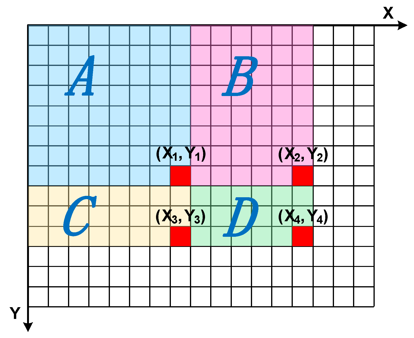
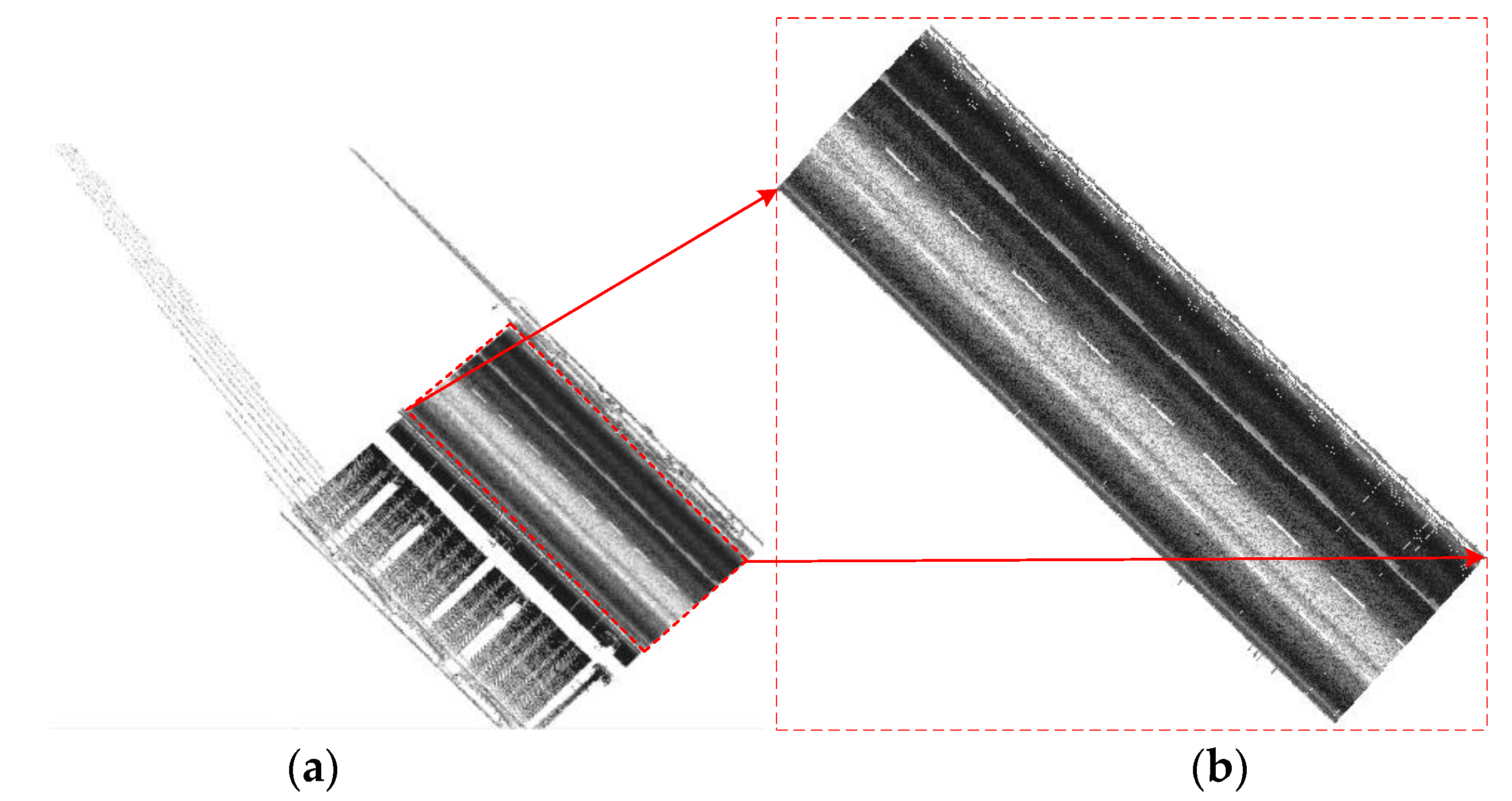
2.2.1. Rasterization of Pavement Point Clouds

In order to make the point clouds adapt to the method of image processing, it is necessary to transfer point clouds into rasterization images. To this end, the inverse distance weighted interpolation (IDW) algorithm is adopted. The basic idea of inverse distance interpolation is that the pixel value of each grid is determined by the intensity of its surrounding point clouds. Two factors need to be considered for the realization of IDW. They are radius of the interpolation and the selection method of the weight of each point cloud lying in the inner interpolation radius.

Assume that the coordinates of a laser point on a pavement are $P_i(X_i,Y_i,H_i,I_i)$, and $I_i$ represents the corresponding reflection intensity of the laser point. Assume that the resolution of the rasterization image is $D_{pixel}$ and the radius of the interpolation is $R_{IDW}$. Then, the size of the rasterization image is determined by Equation (13).

$$\{\begin{array}{c}Width=\left[\frac{maxX-minX}{R_{pixel}}\right]\\ Height=\left[\frac{maxY-minY}{R_{pixel}}\right]\end{array}$$

(13)

where $minX=min\left(X_i\right)$, $maxX=max\left(X_i\right)$, $minY=min\left(Y_i\right)$, $maxY=min\left(Y_i\right)$.

The plane distance between some point cloud $P_k(X_k,Y_k,H_k,I_k)$ (as is shown in Figure 4) and the center of the pixel $Pixe{l}_{\left(m,n\right)}$ is determined by Equation (14).

$$d_{\left(m,n,k\right)}=\sqrt{{\left(X_k-\left(minX+\frac{\left(2m-1\right)R_{pixel}}{2}\right)\right)}^2+{\left(Y_k-\left(minY+\frac{\left(2n-1\right)R_{pixel}}{2}\right)\right)}^2}$$

(14)

when the nth power of the reciprocal of the distance $d_{\left(m,n,k\right)}$ is assumed to be the weight of the interpolation, the intensity of the point ($P_k$) to be interpolated is determined by Equation (15).

$$I_{\left(m,n\right)}=\frac{\sum {\left(\frac{1}{d_{\left(m,n,k\right)}}\right)}^t{I}_k}{\sum {\left(\frac{1}{d_{\left(m,n,k\right)}}\right)}^t}$$

(15)

The normalization gray value of the pixel $Pixe{l}_{\left(m,n\right)}$ is calculated by Equation (16).

$$G_{\left(m,n\right)}=\frac{I_{\left(m,n\right)}-minI}{maxI-minI}$$

(16)

where $minI=min\left(I_{\left(i,j\right)}\right)$, $maxI=max\left(I_{\left(i,j\right)}\right)$, $n\le i\le m$, $n\le j\le m$.

2.2.2. Adaptive Threshold Segmentation

After the original point clouds are transformed into rasterization images, it is necessary to transform rasterization images into binary images in order to extract the road marking point clouds. The image binarization method used in this paper is adaptive threshold segmentation, which was proposed by Wellner [15] in 1993. The main idea of the adaptive threshold is that the gray value of each pixel of one image is determined by the gray value of its surrounding pixels. In [16], the authors improved the method proposed by Wellner. They combined adaptive threshold segmentation with integral image for the purpose of obtaining a binary image. The sum of pixel gray values in any rectangular region of one image can be easily calculated by using the integral image. For instance, in Figure 5, the sum of pixel gray values in rectangle region $D$ can be calculated by Equation (17). Adaptive threshold segmentation will become easier with the help of the integral image.

$$D=int{I}_{\left(x_4,{\mathrm{y}}_4\right)}+int{I}_{\left(x_1,{\mathrm{y}}_1\right)}-int{I}_{\left(x_2,{\mathrm{y}}_2\right)}-int{I}_{\left(x_3,{\mathrm{y}}_3\right)}$$

(17)

where $\left(x_i,{\mathrm{y}}_i\right), i=1,2,3,4$ represent the pixel coordinates of the lower right corner of a rectangular area.

Adaptive threshold segmentation is realized by comparing the gray value of a pixel $p_i\left(x_i,y_i\right)$ (see Figure 6) with the average gray value of pixels lying in its surrounding rectangular area (yellow area in Figure 6). If the gray value of the pixel is greater than the average gray value of its surrounding pixels, it can be considered as the foreground pixel, otherwise it is considered as the background pixel.

Suppose that parameter $s$ (see Figure 6) and parameter $t$ (the value of t is greater than 0 and less than 1) represents the background radius and the segmentation coefficient, respectively; then, the sum of pixel gray values in the rectangular area with $P_i$ as the center and $2s+1$ as the side length is determined by Equation (18).

$$su{m}_i=int{I}_{\left(x_i+s,y_i+s\right)}+int{I}_{\left(x_i-s-1,y_i-s-1\right)}-int{I}_{\left(x_i-s-1,y_i+s\right)}-int{I}_{\left(x_i+s,y_i-s-1\right)}$$

(18)

At this point, the gray value of a pixel after adapting adaptive threshold segmentation is determined by Equation (19).

$$I_{\left(x_i,y_i\right)}^{\prime }=\{\begin{array}{c}1, I_{\left(x_i,y_i\right)}>\frac{su{m}_i}{{\left(2s+1\right)}^2}\ast t\\ 0, others\end{array}$$

(19)

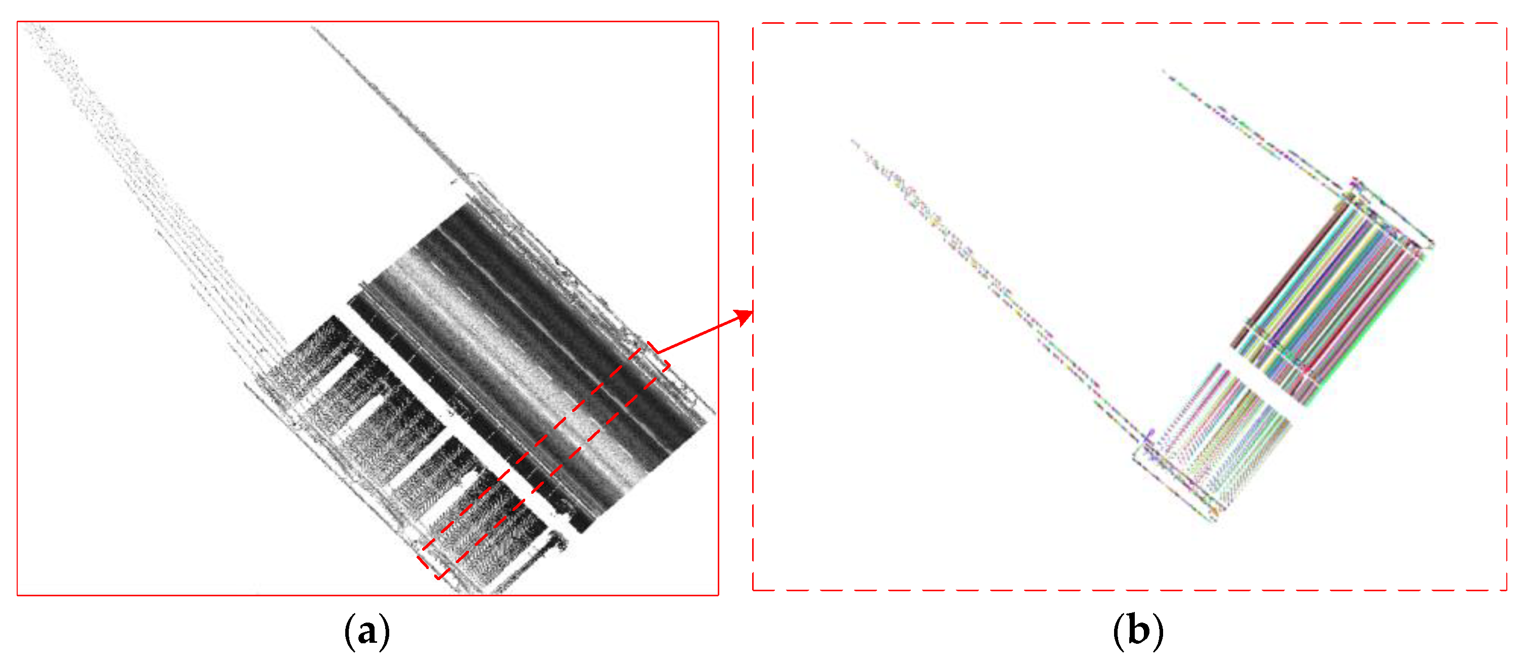
2.2.3. Euclidean Clustering of Road Marking Point Clouds

In the former section, the foreground pixels of the binary image, which represent pavement markings, are extracted according to adaptive threshold segmentation. The subspace clustering method [17] can be used for clustering in high-dimensional space, while the Euclidean clustering algorithm based on distance is only needed for clustering in this paper. Firstly, we restore the pavement markings point clouds from the binary image; then, based on the Euclidean distance between the coordinates of the point clouds, Euclidean clustering is applied to cluster road marking point clouds into point cloud clusters lying on different positions. Let the pavement point clouds be divided into $P=\left\{P_i\left(X_i,Y_i,H_i,I_i\right), i=1,2,3\cdots \right\}$. Let the segmentation distance parameter be $D$; then, the specific method is as follows.

(1)

Starting from any point $P_i$ in point set $P$, add $P_i$ to the point set $C$.

(2)

Add the points in the range of $D$ centered on $P_i$ into point set $C$, as shown in Figure 7a.

(3)

Repeat step (2) with each newly added point in point set $C$ as the center, until no new points are added to point set $C$, as shown in Figure 7b,c.

(4)

Start a new clustering by repeating steps (1)–(3) from the remaining points in P until all points are handled, as shown in Figure 7d.

Although Euclidean clustering is used to cluster point clouds into independent point cloud clusters, the real classification of these clusters is still unknown. For the purpose of obtaining semantic information of these clusters, geometric attribute filtering [18] is utilized to recognize solid lines. The remaining point cloud road markings are recognized by the deep learning network PointNet++ [19].

In order to identify solid lines from all point cloud clusters, the minimum bounding rectangle (MBR) of each point cloud cluster is calculated. Some attributes of the cluster are defined by the MBR of each point cloud cluster. We distinguish solid lines from point cloud clusters by restricting attributes of MBR. The following two parameters, i.e., $a$ and $\beta$ in Equation (20), are defined for the purpose of distinguishing solid lines from all point cloud clusters.

$$\beta =\frac{a}{b}$$

(20)

where $\beta$ represents the length-width ratio, $a$ represents the longer side of the MBR, and $b$ represents the shorter side of the MBR.

Solid lines can be removed from all point cloud clusters when they are recognized from all clusters. There are five other kinds of road markings in the remaining road markings. They are dashed lines, guidelines, straight arrows, left turn arrows and right turn arrows. At present, when it comes to point cloud semantic recognition, many deep learning networks such as PointNet++, pointcnn (Li et al., 2018) [20] and KPconv (Thomas et al., 2019) [21] are applied to indoor scene point clouds or outdoor large scene point clouds. These deep learning networks are mainly used for semantic recognition of large-scale objects such as buildings, trees, cars and pedestrians. Few studies have applied a deep learning network to semantic segmentation of road markings. In this paper, the classification module of the deep learning network PointNet++ is applied to identify remaining clusters.

2.3. Road Markings Vectorization

The former part of this process only recognizes each separate road marking cluster. It still fails to form complete and directional road markings. In practical applications, such as high-precision maps for automatic driving, these separate road marking clusters need to be vectorized. This part will consider the spatial relationship among the identified point cloud clusters to determine the complete road marking. The vectorization of road markings in this paper mainly refers to the vectorization of the following three kinds of road markings: solid lines, dashed lines and guidelines. The method used in the process of vectorizing solid lines and dashed lines is a line segment self-growth algorithm based on an endpoint search. The method of vectorizing guidelines is a alpha shape algorithm [22].

In order to describe the line segment self-growth algorithm more conveniently, several parameters need to be defined. The parameter $r_{search}$ represents the search distance. The parameter $A_{search}$ represents the search angle. The parameter $S_i$ represents the similarity threshold between two clusters. The similarity measure between two clusters is determined by Equation (21).

$$Similarity=\sqrt{\frac{{\left(1-\frac{\left|a-a^{\prime }\right|}{a+a^{\prime }}\right)}^2+{\left(1-\frac{\left|b-b^{\prime }\right|}{b+b^{\prime }}\right)}^2}{2}}$$

(21)

where $a$, $b$, $a^{\prime }$, $b^{\prime }$ represents the length and the width of the MBR between two clusters to be measured, respectively.

Taking the vectorization of the dashed line clusters as an example, the specific steps of the line segment self-growth algorithm are as follows.

• Determination of the growth point. Suppose the total number of road marking clusters is n. Starting from the arbitrary cluster cluster_i(i∈[1,n]). If the distance between the MBR center of cluster_j(j∈[1,n], j≠i) and the MBR center of cluster_i is less than r (r = 20 m), cluster_j will be put into set clusterSet_r, as shown in Figure 8.
• Determination of the direction of growth. The direction of growth is determined by the direction of the vehicle trajectory, as shown in Figure 9.
• Firstly, calculate the coordinate azimuth $A_{i\_j}$ between the MBR center of cluster_i and the MBR center of the clusters concluded in the set clusterSet_r. Secondly, calculate the difference $angl{e}_{i\_j}$ (see Figure 9) between the azimuth $A_{i\_j}$ and the azimuth of cluster_i. The clusters that satisfy Equation (22) will be put into set clusterSet_A. The parameter $A_{search}$ in this paper is set as 5°.

  $$angl{e}_{i\_j}<A_{search}$$

  (22)

  Thirdly, calculate the difference $angl{e}_{i\_j}\prime$ (see Figure 9) between the azimuth of the cluster_j and the azimuth of the growth direction. The clusters that satisfy Equation (23) will be put into set clusterSet_A’. The parameter A in this paper is set as 5°.

  $$angl{e}_{i\_j}{}^{\prime }<A$$

  (23)
• Calculate the similarity between cluster_i and the cluster concluded in the set clusterSet_A’ according to Equation (21). The clusters that satisfy Equation (24) are named as clusterSet_S_i. The parameter S_i in this paper is set as 0.58.

  $$Similarity>S_i$$

  (24)
• If the set clusterSet_S_i does not exist, the line segment growth will be over. Set the cluster_i to be any unconnected cluster and start a new line segment growth. Repeat steps $i–\mathrm{iii}$ until all of the road marking clusters are connected.
• In set clusterSet_S_i, find out the cluster nearest to cluster_i, and mark it as cluster_j. cluster_j is the next cluster to be connected.
• Update the growth point to the MBR center of cluster_j and repeat the above steps until all of the clusters have been processed.

A flow chart of the line segment self-growth algorithm is shown in Figure 10.

Figure 8. Diagrammatic sketch of the determination of growth point.

Figure 8. Diagrammatic sketch of the determination of growth point.

Figure 9. Diagrammatic sketch of the determination of the growth direction.

Figure 9. Diagrammatic sketch of the determination of the growth direction.

Figure 10. Line self-growth algorithm flow chart.

Figure 10. Line self-growth algorithm flow chart.

3. Experimental Data and Scheme

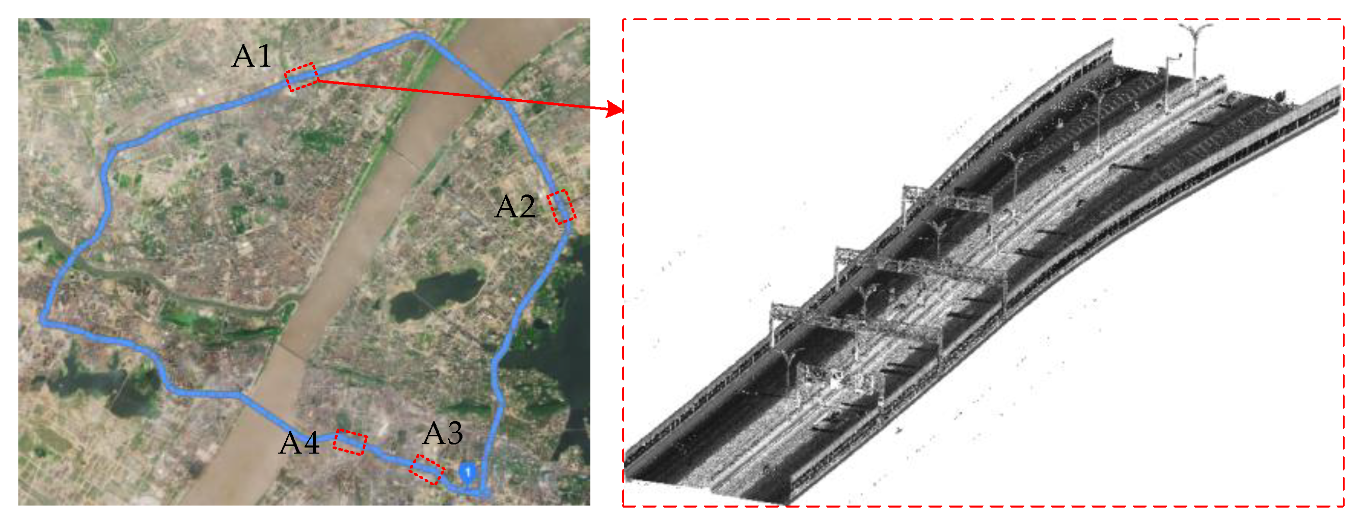
3.1. Experimental Data

On 18 and 24 April 2017, the point cloud data of the second ring road in Wuhan, Hubei Province, were collected by using the mobile laser measurement system. The experiment area covers about 48 km of urban roads, with good overall road conditions and clear road markings. The width of the experimental road is about 15 m. The point clouds data include 3D coordinates and corresponding intensity information. Four test areas are selected to verify the proposed method, each of which is about 160 m long. The experimental area and point clouds diagrammatic sketch of the urban environment is shown in Figure 11. The relevant parameters of the collecting point clouds data is shown in

Table 1. Parameters of point clouds data collection.

Parameter Type	Value
Scanner model	RIEGL VUX-1
Scanning mode	Single line cross section scanning
Vehicle speed	35~40 km/h
Scanning frequency	200 hz
Scanning speed	500,000 points/s
Vertical field of view	330°

.

3.2. Experimental Scheme

The experimental parameters were selected as follows. As previously described in Section 2.1, the parameter $L_d$ should be set to avoid introducing pseudo key points as much as possible. From experience, $L_d$ is generally set to be 1/3 of the road width. $M_l$ is generally set to be half of the road width. $M_n$ is closely related to the density of the scanning line point density, which can be determined by Equation (5). The parameter $M_n$ should be set to exclude non-road boundary points in the key points. The value of the parameter $cH$ should be less than curb height, and in this paper, it is set to 0.08 m. The parameters $mS$ and $fH$ are related to road roughness. The parameter $minN$ is set to half of the number of point clouds lying on a scan line. The values of these parameters are listed in

Table 2. Parameter table for the extraction of road markings.

Parameter	Value	Parameter	Value
$L_d$	5 m	$mS$	25°
$M_l$	7 m	$fH$	0.05 m
$M_n$	650	$minN$	350
$\mathrm{c}H$	0.08 m

.

F-score is a parameter that is used to evaluate the accuracy of road marking extraction. It is calculated by Equations (25)–(27). The method of evaluation is adopted from literature [23].

$$\mathrm{completeness}=\frac{TP}{TP+FN}$$

(25)

$$\mathrm{correctness}=\frac{TP}{TP+FP}$$

(26)

$$\mathrm{F}-\mathrm{score}=\frac{2\ast completeness\ast correctness}{completeness+correctness}$$

(27)

where $TP$, $FN$ and $FP$ represent the pixel counts that are extracted correctly, defectively and redundantly, respectively.

4. Experimental Results

4.1. Pavement Extraction

When the values of the parameters $L_d$, $M_l$ and $M_n$ are set to the values in Table 2, the effect of the extracted scan lines is shown in Figure 12.

In this paper, the parameter $\mathrm{c}H$ is set to 0.08 m. The parameter $mS$ is set to 25 degrees. The smaller the value of $mS$, the stricter the requirement of pavement smoothness is. The parameter $fH$ is set to 0.05 m. As there may be some incorrect extraction of the scan line, a large occlusion may occur in the actual data acquisition. Therefore, the number of scanning line points will be relatively small in this scenario, and the parameter $minN$ needs to be set. Only when equality (28) is satisfied is it considered that the extracted pavement point clouds is effective. The parameter $minN$ is related to scanning density. It is generally set to half of the number of points belonging to one scan line. The value of the parameters $\mathrm{c}H$, $mS$, $fH$ and $minN$ are listed in Table 2. Figure 13 shows the pavement point clouds extracted from the scan line.

$$minN<\max \left\{N_k\right\}$$

(28)

4.2. Rasterization of Pavement Point Clouds

Four sections of roads A1, A2, A3 and A4 (see Figure 11) were selected from the original road point clouds as the test areas, with each section having a length of approximately 160 m. Following the method described in Section 2.1, the pavement point clouds are extracted from the four original road point clouds and then transformed into raster images. We tried different values of the parameter $t$ in Equation (15) and found that the best result can be obtained when parameter $t$ equals 3. The point interval among the point clouds is about 0.015 m in our experiment, the pixel resolution of the rasterization image is set to 0.05 m, i.e., $D_{pixel}=5 cm$. In order to avoid pixel holds to the greatest extent, the interpolation radius is set to 0.15 m, i.e., $R_{IDW}=0.15 m$. Figure 14 shows a schematic diagram of the four sections of pavement point clouds for A2, A3, A4 and A1 converted into raster images.

To some extent, IDW can counteract the influence of an uneven intensity value on the extraction of road marking.

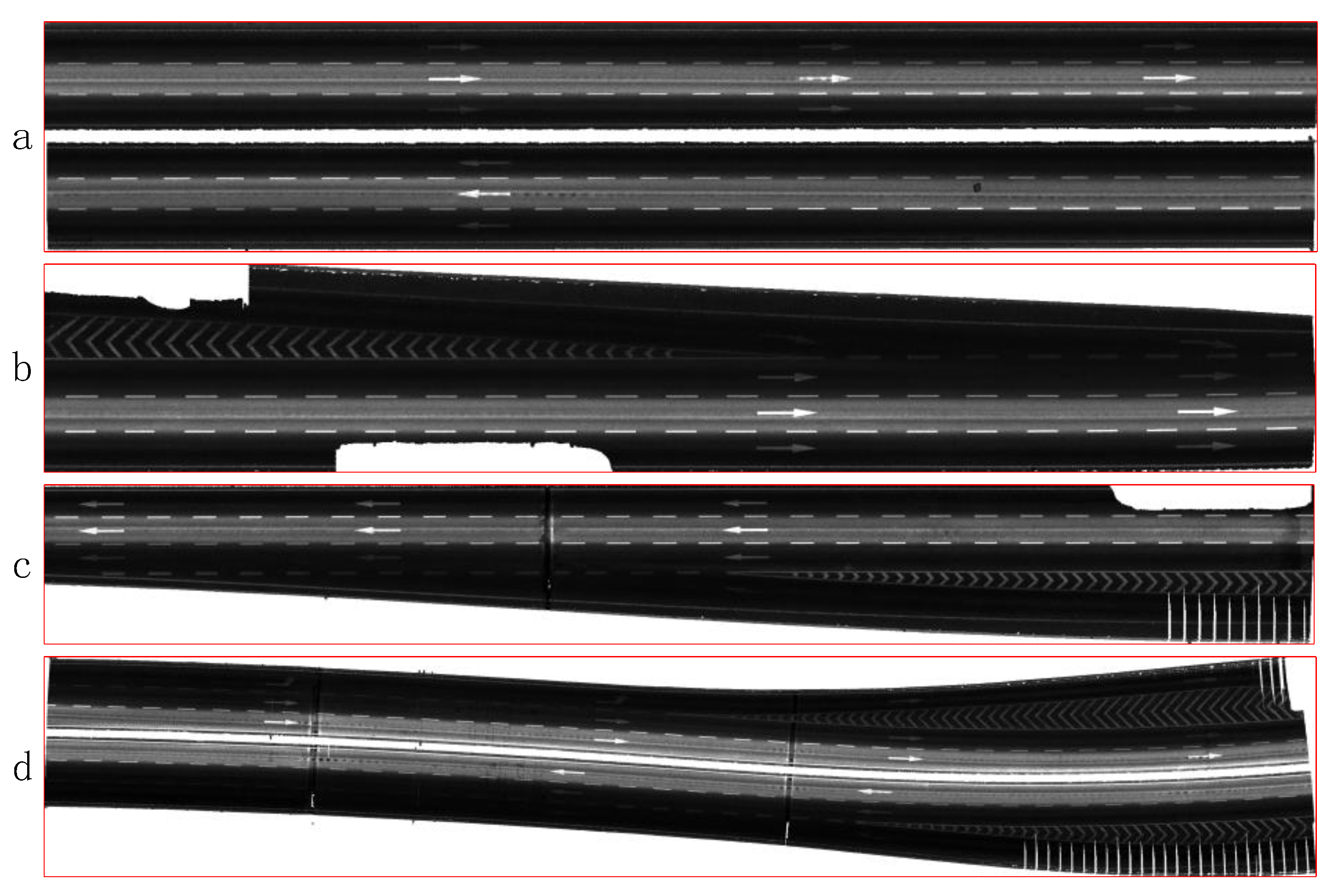
4.3. Binarization of Pavement Image

An adaptive threshold segmentation depicted in Section 2.2.2 is used to transform the raster images into binary images. The optimum parameters, i.e., background radius (s) and segmentation coefficient (t), are used to convert the raster images into binary images in the corresponding test area (as shown in Figure 15). The method for obtaining the optimal adaptive threshold segmentation parameters s and t is discussed in Section 5. As can be seen from Figure 15, some pavement point clouds are incorrectly marked as road marking point clouds due to road wear, as shown in the red rectangular box, and some road markings are defective due to occlusion, as shown in the blue rectangular box.

4.4. Euclidean Clustering

After the raster images are converted into binary images, the corresponding original point clouds can be recovered from the foreground pixels of the binary images. These original point clouds are the road marking point clouds that are extracted. In order to identify the type of road markings, it is necessary to cluster the discrete point clouds of road markings into different point cloud settlements. In Section 2.2.3, the setting of the clustering radius should separate different types of road markings as much as possible. According to the distribution characteristics of road markings, the clustering radius D is set to 0.5 m. This clustering radius can separate different road markings as much as possible. The result of applying Euclidean clustering into extracted road marking point clouds is shown in Figure 16. Test areas a, b, c and d correspond to four test areas, A2, A3, A4 and A1, respectively. Different colors represent different clustering categories. We can see that the same solid line may be clustered into different point cloud settlements due to factors such as occlusion and pavement wear during data acquisition. Some noise is also clustered into the point cloud clusters, which may have some influence on road marking recognition.

4.5. Recognition of Road Markings

In Section 2.3, the threshold of parameter $a$ is set to 7 m, and the threshold of parameter β is set to 20. When $a$ is greater than 7 m and β of some cluster is greater than 20, the solid line can be discriminated from all of the point cloud clusters (see Figure 17).

The deep learning network PointNet++ is applied on the remaining clusters. The number of dashed lines with labels included in the training data is 2060, and the number of guidelines, straight arrows, left turn arrows and right turn arrows included in the training data is 2045, 2045, 2045 and 2045, respectively. These training data are labeled with corresponding labels. The total number of labeled road markings used for training is 10,240. They are fed into the classification module of PointNet++ for training. The testing data contain 412 dashed lines with labels, and the number of guidelines, straight arrows, left turn arrows and right turn arrows included in the testing data is 409, 409, 409 and 409, respectively. These testing data are also labeled with corresponding labels. The total number of road markings used for testing is 4096. Another four areas of unlabeled road markings are used as prediction data. The semantic recognition result is shown in Figure 17. The identified dashed lines are marked in red. The identified solid lines are marked in cyan. The identified guidelines are marked in yellow. The identified right turn arrows are marked in blue. The identified straight arrows are marked in pink. Road markings that are misclassified are surrounded by cyan boxes. In this paper, the road marking identification results are evaluated using the precision, recall and F-score. Quantitative test results are shown in

Table 3. Evaluation of road marking recognition.

Category	Total	TP	FN	FP	Precision	Recall	F-Score
Broken line	325	310	16	3	0.95	0.99	0.97
Guideline	4	4	0	4	1.00	0.5	0.66
Straight arrow	38	37	1	13	0.97	0.74	0.84
Left turn arrow	1	0	1	0	0	-	-
Right turn arrow	3	3	0	0	1	1	1

.

From the result of road markings recognition, we can see that some dashed lines are misclassified as straight arrows due to their similarity in shape, as are left turn arrows and guidelines. All of the solid lines and guidelines are classified correctly. There is one left turn arrow, which is mistakenly identified as a guideline; therefore, there are no values for recall and F-score. There is still some pavement noise, which is misclassified as dashed lines. This road noise may be caused by the long-term wear of the pavement.

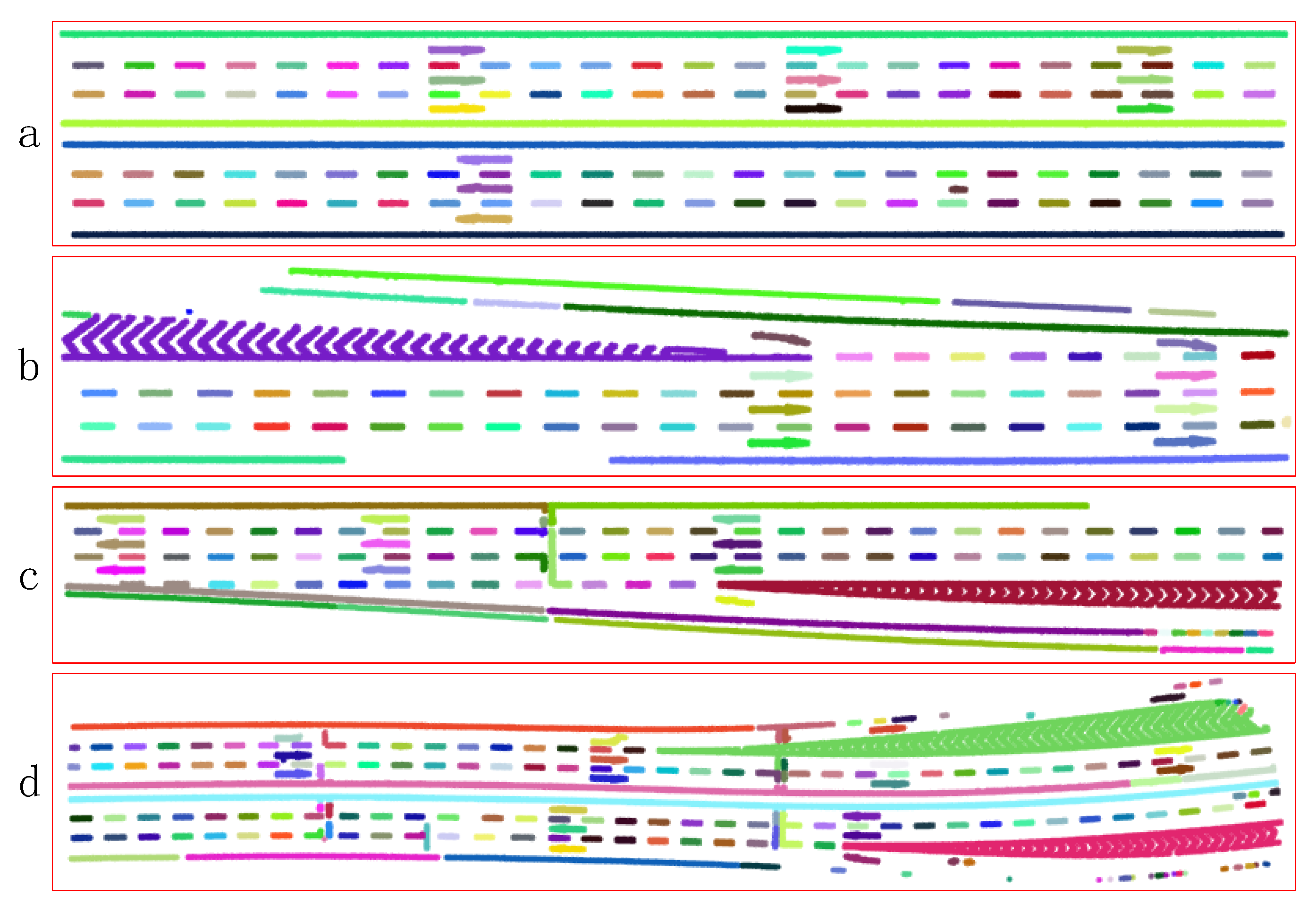
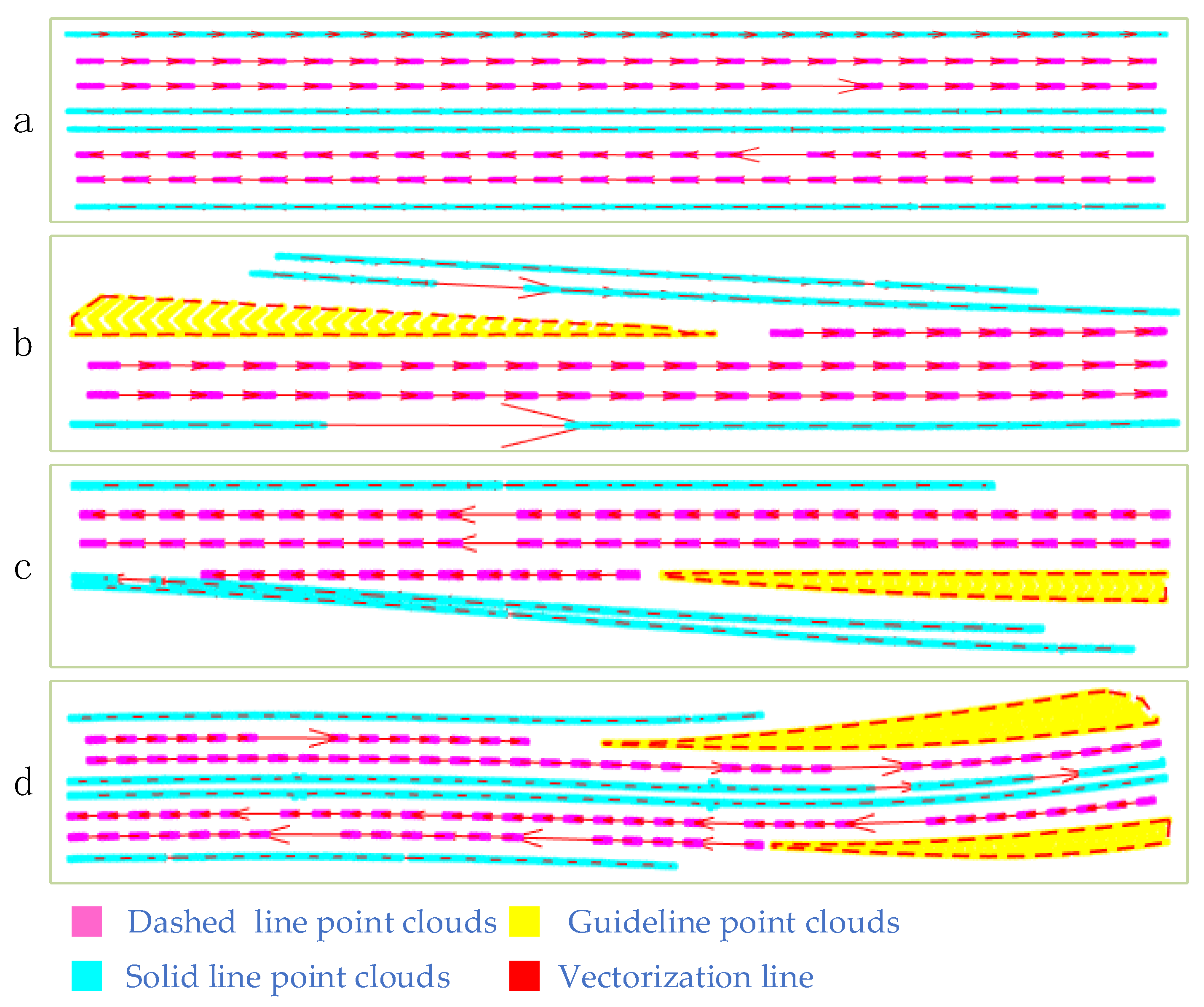
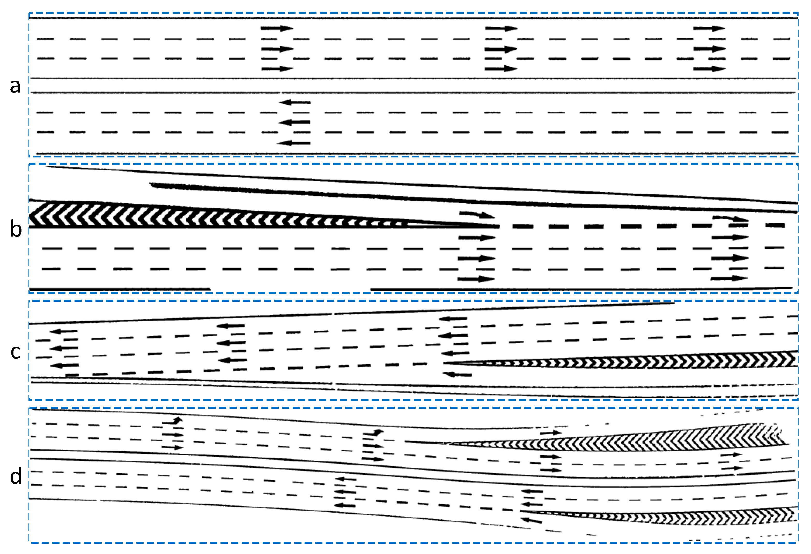
4.6. Vectorization of Road Markings

Section 2.3 depicts the process of vectorization of road markings for dashed lines. In fact, the solid lines can be divided into numerous dashed line clusters. Therefore, the vectorization of solid line clusters is similar to the vectorization of the dashed lines. The empirical values of the search angle, search distance and similarity are given first (in Section 2.3) and then updated according to the partial sample data. The alpha shape algorithm is used to vectorize the guidelines. As shown in Figure 18, all dashed lines, solid lines and guidelines correctly identified in the previous section are correctly vectorized.

5. Discussion

In order to quantitatively analyze the influence of the parameters s and t (Section 4.3) on the road marking extraction results, the road markings are extracted manually from the original point clouds, corresponding to the A2, A3, A4 and A1 test areas (as shown in Figure 19).

The road markings extracted manually are compared with those extracted automatically in Section 4.3 pixel by pixel, and a different F-score is calculated when the parameters $s$ and the parameter $t$ are different values in respective sections of road. The parameters that maximize the F-score are the optimum parameters that are searched for, as described in Section 4.3. The method of calculating the F-score values is described in Section 3.2. We traverse different values of the parameter $s$ in the interval [5, 50] with sub-interval 1, and we also traverse different values of the parameter $t$ in the interval [0.5, 1.8] with sub-interval 0.01, aiming to determine the parameter F-score under the condition of different values of the parameters $s$ and $t$.

Figure 20 shows the surface graph of the parameter F-score with respect to parameters $s$ and $t$. We can see the obvious extreme value ridge, which is relatively gentle and shows that the parameters $s$ and $t$ have a relatively broad and appropriate range. In fact, the extreme value ridge is the maximum of the F-score in the $t$ direction. It can also be seen from Figure 20 that the F-score is not sensitive to the change of the parameter $s$, but is sensitive to the change of segmentation coefficient $t$. As the parameter $s$ increases, the parameter $t$ maximized F-score also gradually increases. The higher the value of correctness is, the greater the proportion of correctly extracted road marking pixels is in the extracted road marking pixels. The greater the value of completeness is, the greater the proportion of pixels that are correctly extracted from the original road marking pixels. Generally speaking, when the parameter $s$ is certain, the parameter $t$ and correctness values are higher and the completeness value is lower. The quantitative evaluation of road marking extraction is shown in

Table 4. The quantitative evaluation of road marking extraction.

Test Data	$(\mathit{s}\mathit{,}\mathit{t})$	Completeness	Correctness	F-Score
a	(7, 1.28)	0.94	0.73	0.83
b	(14, 1.38)	0.86	0.79	0.82
c	(13, 1.43)	0.82	0.83	0.83
d	(13, 1.36)	0.90	0.78	0.84

. In general, the overall accuracy of road marking extraction is about 0.83, and the errors are mainly concentrated near the road boundary with a sparse point density.

In Figure 15 (Section 4.3), false positive error means that some road pavement point clouds are wrongly marked as road marking point clouds. The reason for this may be that the point cloud intensity value in the wear area is high due to the pavement wear. The false negative error represents a defect in the road marking point clouds, which may be caused by the blocking of vehicles during data collection. This deficiency can be remedied by scanning the pavement again.

Despite the fact that the point clouds recovered from false positive pixels belong to noise point clouds, after the implementation of point cloud clustering, the included angle between these clusters and the driving trace is greater than 45 degrees. During point cloud clustering recognition, a certain threshold is set for the included angle, and the noise clusters can be removed. In the vectorization stage of point cloud clustering, the noise clusters that are approximately parallel to the driving trace are removed according to the search angle threshold in the line segment self-growth algorithm.

The advantages of the proposed method are as follows. On the one hand, road markings are automatically extracted from the original point clouds without manual intervention or data preprocessing. On the other hand, the line segment self-growing algorithm proposed in this paper can resist the influence of noise clustering to a certain extent. The disadvantages of the proposed method lie in the fact that the missing of road point clouds caused by vehicle occlusion cannot be recovered at present, which affects the completeness of road marking extraction to a certain extent.

In this paper, the proposed method is suitable for extracting expressway road markings but may not be suitable for urban road marking extraction. At this time, the deep learning method can be considered for the semantic segmentation of 3D point clouds to separate the pavement from the original point clouds. In the process of point cloud data collection, mutual occlusion between vehicles or defective road markings would affect the accuracy of road marking extraction. However, a small number of defective road markings would not affect vectorization of the road markings, for example, vectorization of the dashed lines does not require participation of all the dashed line segments. In this paper, in order to extract road marking point clouds from pavement point clouds, the pavement point clouds are converted into raster images, and then, the raster images are converted into binary images, from which the road marking point clouds are recovered. An advantage of rasterization of pavement point clouds is that this method of image processing can be used to extract road marking point clouds; a disadvantage of this method is that if the parameters of adaptive threshold segmentation are not set properly, road noise may be introduced.

6. Conclusions

This paper extracts and recognizes road markings from vehicle-borne laser point clouds. Firstly, each scan line is extracted from initial point clouds based on the distance mutation between adjacent points. Pavement point clouds are extracted from scan lines based on the mutation of geometry, such as elevation and slope, on the boundary of the scan lines that represent the road section. Some geometry threshold values such as curb height, curb slope and fluctuation degree of pavement, are set up for the purpose of extracting pavement point clouds. Secondly, IDW is utilized to transform pavement point clouds into a raster image with a certain resolution. Adaptive threshold segmentation is used to extract road marking point clouds from the raster image. Then, the solid lines are recognized from point cloud clusters by geometric attribute filtering. The classification module of the deep learning framework PointNet++ is used to distinguish the specific category of the remaining road markings. Finally, because less research has been done on the vectorization of identified road markings, the line segment self-growth algorithm based on an endpoint search is proposed to vectorize the identified dashed lines and solid lines.

Due to the influence of road noise and occlusion, the overall accuracy of road marking extraction needs be improved. This paper only considers road marking extraction in a highway environment and does not consider road marking extraction in an urban road environment. Semantic segmentation only considers the markings on the road, not the geographical entities on both sides of the road. Future research will focus on the semantic segmentation of other road traffic objects in expressway and urban road environments.

References

1. Cheng, Y.; Patel, A.; Wen, C.; Bullock, D.; Habib, A. Intensity Thresholding and Deep Learning Based Lane Marking Extraction and Lane Width Estimation from Mobile Light Detection and Ranging (LiDAR) Point Clouds. Remote Sens. 2020, 12, 1379. [Google Scholar] [CrossRef]
2. Li, Z.; Cai, Z.; Xie, J.; Ren, X. Road markings extraction based on threshold segmentation. In Proceedings of the IEEE 2012 9th International Conference on Fuzzy System and Knowledge Discovery (FSKD)—Chongqing, Sichuan, Chian, 29–31 May 2012; pp. 1924–1928. [Google Scholar]
3. Chen, T.; Chen, Z.; Shi, Q.; Huang, X. Road marking detection and classification using machine learning algorithms. In Proceedings of the 2015 IEEE Intelligent Vehicles Symposium (IV), Seoul, Korea, 28 June–1 July 2015; pp. 617–621. [Google Scholar]
4. Rebut, J.; Bensrhair, A.; Toulminet, G. Image segmentation and pattern recognition for road marking analysis. In Proceedings of the 2004 IEEE International Symposium on Industrial Electronics, Ajaccio, France, 4–7 May 2004; Volume 1, pp. 727–732. [Google Scholar]
5. Jung, S.; Youn, J.; Sull, S. Efficient lane detection based on spatiotemporal images. IEEE Trans. Intell. Transp. Syst. 2015, 17, 289–295. [Google Scholar] [CrossRef]
6. Hernández, D.C.; Seo, D.; Jo, K.-H. Robust lane marking detection based on multi-feature fusion. In Proceedings of the 2016 9th International Conference on Human System Interactions (HSI), Portsmouth, UK, 6–8 July 2016; pp. 423–428. [Google Scholar]
7. Azimi, S.M.; Fischer, P.; Körner, M.; Reinartz, P. Aerial LaneNet: Lane-marking semantic segmentation in aerial imagery using wavelet-enhanced cost-sensitive symmetric fully convolutional neural networks. IEEE Trans. Geosci. Remote Sens. 2018, 57, 2920–2938. [Google Scholar] [CrossRef] [Green Version]
8. Yan, L.; Liu, H.; Tan, J.; Li, Z.; Xie, H.; Chen, C. Scan line based road marking extraction from mobile LiDAR point clouds. Sensors 2016, 16, 903. [Google Scholar] [CrossRef] [PubMed]
9. Guan, H.; Li, J.; Yu, Y.; Ji, Z.; Wang, C. Using mobile LiDAR data for rapidly updating road markings. IEEE Trans. Intell. Transp. Syst. 2015, 16, 2457–2466. [Google Scholar] [CrossRef]
10. Yu, Y.; Li, J.; Guan, H.; Jia, F.; Cheng, W. Learning hierarchical features for automated extraction of road markings from 3-D mobile LiDAR point clouds. IEEE J. Sel. Top. Appl. Earth Obs. Remote Sens. 2015, 8, 709–726. [Google Scholar] [CrossRef]
11. Wang, H.; Luo, H.; Wen, C.; Cheng, J.; Li, P. Road Boundaries Detection Based on Local Normal Saliency from Mobile Laser Scanning Data. IEEE Geosci. Remote Sens. Lett. 2015, 12, 2085–2089. [Google Scholar] [CrossRef]
12. Guan, H.; Li, J.; Yu, Y.; Wang, C.; Chapman, M.; Yang, B. Using mobile laser scanning data for automated extraction of road markings. ISPRS J. Photogramm. Remote Sens. 2014, 87, 93–107. [Google Scholar] [CrossRef]
13. Yang, B.; Fang, L.; Li, Q.; Li, J. Automated extraction of road markings from mobile LiDAR point clouds. Photogramm. Eng. Remote Sens. 2012, 78, 331–338. [Google Scholar] [CrossRef]
14. Ma, L.; Li, Y.; Li, J.; Yu, Y.; Junior, J.M.; Gonçalves, W.N.; Chapman, M.A. Capsule-based networks for road marking extraction and classification from mobile LiDAR point clouds. IEEE Trans. Intell. Transp. Syst. 2021, 22, 1981–1995. [Google Scholar] [CrossRef]
15. Wellner, P.D. Adaptive Thresholding for the DigitalDesk. Xerox 1993. [Google Scholar]
16. Bradley, D.; Roth, G. Adaptive thresholding using the integral image. J. Graph. Tools 2007, 12, 13–21. [Google Scholar] [CrossRef]
17. Yao, J.; Cao, X.; Zhao, Q.; Meng, D.; Xu, Z. Robust subspace clustering via penalized mixture of Gaussians. Neurocomputing 2018, 278, 4–11. [Google Scholar] [CrossRef]
18. Yao, L.; Chen, Q.; Qin, C.; Wu, H.; Zhang, S. Automatic Extraction of Road Markings from Mobile Laser-Point Cloud Using Intensity Data. Int. Arch. Photogramm. Remote Sens. Spat. Inf. Sci. 2018, XLII-3, 2113–2119. [Google Scholar] [CrossRef] [Green Version]
19. Qi, C.; Yi, L.; Su, H.; Guibas, L. PointNet++: Deep Hierarchical Feature Learning on Point Sets in a Metric Space. arXiv 2017, arXiv:1706.02413. [Google Scholar]
20. Li, Y.; Bu, R.; Sun, M.; Wu, W.; Di, X.; Chen, B. PointCNN—Convolution On X-Transformed Points. Adv. Neural Inf. Process. Syst. 2018, 31, 828–838. [Google Scholar]
21. Thomas, H.; Qi, C.; Deschaud, J.; Marcotegui, B.; Goulette, F.; Guibas, L. KPConv-Flexible and Deformable Convolution for Point Clouds. In Proceedings of the IEEE/CVF International Conference on Computer Vision, Seoul, Korea, 27 October–2 November 2019; pp. 6410–6419. [Google Scholar]
22. Edelsbrunner, H.; Kirkpatrick, D.; Seidel, R. On the shape of a set of points in the plane. IEEE Trans. Inf. Theory 1983, 29, 551–559. [Google Scholar] [CrossRef] [Green Version]
23. Cheng, M.; Zhang, H.; Wang, C.; Li, J. Extraction and Classification of Road Markings Using Mobile Laser Scanning Point Clouds. IEEE J. Sel. Top. Appl. Earth Obs. Remote Sens. 2017, 10, 1182–1196. [Google Scholar] [CrossRef]
Figure 1. The flowchart of the data process of road markings.
Remotesensing 13 02612 g001
Figure 2. (a) Scan line; (b) Distance between scanning points; (c) Variation of distance between scanning points.
Remotesensing 13 02612 g002
Figure 3. Sketch map of pavement point cloud extraction based on scan line.
Remotesensing 13 02612 g003
Figure 4. Sketch map of Inverse Distance Weighted interpolation.
Remotesensing 13 02612 g004
Figure 5. The principle of the integral image.
Remotesensing 13 02612 g005
Figure 6. The sketch map of the adaptive threshold segmentation.
Remotesensing 13 02612 g006
Figure 7. Diagrammatic sketch of Euclidean clustering. (ac) The points before Euclidean clustering is complete; (d) The points after Euclidean clustering is complete. 2.3. Road Markings Recognition.
Remotesensing 13 02612 g007
Figure 11. Experimental area and point clouds diagrammatic sketch of urban environment.
Remotesensing 13 02612 g011
Figure 12. (a) Original point cloud; (b) scan line extracted from the original point cloud.
Remotesensing 13 02612 g012
Figure 13. Pavement point cloud extraction. (a) Original point cloud; (b) pavement point cloud.
Remotesensing 13 02612 g013
Figure 14. The raster image of the point cloud. (a) Raster image converted from area A2; (b) Raster image converted from area A3; (c) Raster image converted from area A4; (d) Raster image converted from area A1.
Remotesensing 13 02612 g014
Figure 15. The result of the adaptive threshold segmentation. (a) Binary image converted from Figure 14a; (b) Raster image converted from Figure 14b; (c) Raster image converted from Figure 14c; (d) Raster image converted from Figure 14d.
Remotesensing 13 02612 g015
Figure 16. The result of Euclidean clustering (different colors represent different clustering categories). (a) Euclidean clustering result of Figure 15a; (b) Euclidean clustering result of Figure 15b; (c) Euclidean clustering result of Figure 15c; (d) Euclidean clustering result of Figure 15d.
Remotesensing 13 02612 g016
Figure 17. The result of semantic recognition of road markings. (a) The result of semantic recognition of Figure 16a; (b) The result of semantic recognition of Figure 16b; (c) The result of semantic recognition of Figure 16c; (d) The result of semantic recognition of Figure 16d.
Remotesensing 13 02612 g017
Figure 18. Road markings vectorization for dashed lines and solid lines. (a) The result of vectorization of Figure 17a; (b) The result of vectorization of Figure 17b; (c) The result of vectorization of Figure 17c; (d) The result of vectorization of Figure 17d.
Remotesensing 13 02612 g018
Figure 19. The road marking extracted manually. (a) Road marking extracted from Figure 14a; (b) Road marking extracted from Figure 14b; (c) Road marking extracted from Figure 14c; (d) Road marking extracted from Figure 14d.
Remotesensing 13 02612 g019
Figure 20. The surface graph of the parameter F-score with respect to parameters s and t . (a) The surface graph calculated from Figure 19a; (b) The surface graph calculated from Figure 19b; (c) The surface graph calculated from Figure 19c; (d) The surface graph calculated from Figure 19d.
Remotesensing 13 02612 g020