Mapping 30 m Fractional Forest Cover over China’s Three-North Region from Landsat-8 Data Using Ensemble Machine Learning Methods

Abstract

The accurate monitoring of forest cover and its changes are essential for environmental change research, but current satellite products for forest coverage carry many uncertainties. This study used 30-m Landsat-8 data, and aggregated 1-m GaoFen-2 (GF-2) satellite images to construct the training samples and used multiple machine learning algorithms (MLAs) to estimate the fractional forest cover (FFC) in China’s Three North Region (TNR). In this study, multiple MLAs were merged to construct stacked generalization (SG) models based on the idea of SG, and the performances of the MLAs in the FFC estimation were evaluated. The results of the 10-fold cross-validation showed that all non-linear algorithms had a good performance, with an R² value of greater than 0.8 and a root-mean square error (RMSE) of less than 0.05. In the bagging ensemble, the random forest (RF) (R² = 0.993, RMSE = 0.020) model performed the best and in the boosting ensemble, the light gradient boosted machine (LGBM) (R² = 0.992, RMSE = 0.022) performed the best. Although the evaluation index of the RF is slightly better than that of the LGBM, the independent validation results show that the two models have similar performances. The model evaluation results of the independent datasets showed that, in the SG model, the performance of the SG(LGBM) (R² = 0.991, RMSE = 0.034) was better than that of the single or non-ensemble model. Comparing the FFC estimates of our model with those of existing datasets showed that our model exhibited more forest spatial distribution details and higher accuracy in complex landscapes. Overall, in this study, the method of using high-resolution remote sensing (RS) images to extract samples for FFC estimation is feasible. Our results demonstrate the potential of the ensemble MLAs to map the FFC. The research results also show that among many MALs, the RF algorithm is the most suitable algorithm for estimating FFC, which provides a reference for future research.

1. Introduction

Forests are the ecosystems with the richest biodiversity on land and represent an important factor affecting global carbon, water cycles, biodiversity, land-use change, and climate change [1,2,3,4,5,6,7]. China’s Three-North Shelter Forest Program (TNSFP) [8] is the largest artificial afforestation project in the world, covering more than 40% of China’s land area and serving as an important ecological barrier in northern China [9,10]. TNSFP not only holds important economic benefits but also plays an important role in preventing wind, fixing sand, regulating water and heat, improving the microclimate, soil, and water conservation, reducing natural disasters, and realizing the sustainable and healthy development of the ecological environment [11]. Owing to the fragility and complexity of the ecological environment in the Three-North Region (TNR), the vegetation ecosystem in this region is affected by ever-changing land use/cover, and forest coverage information is an important factor used to characterize the ecological environment. It is of great significance to obtain timely and accurate forest coverage information and temporal and spatial changes in this region to study the ecological environment and vegetation coverage changes, sustainable management of land use and forests, and climate change in the TNR [12,13,14].

Although several studies extracted forest cover information from 1-km AVHRR, 500-m and 250-m MODIS, and other remote sensing (RS) images [15,16,17], in heterogeneous forests areas, forests and forest disturbances might be small and fragmented, resulting in many pixels that are spectrally mixed between disturbed forests, undisturbed forests, and non-forest classes [18,19]. In addition, in the change products defined based on the forest cover change, forest disturbances smaller than the pixel scale may be ignored, and the classification results cannot fully represent the intra-class heterogeneity problem within a certain pixel. Therefore, coarse-resolution RS images have obvious limitations in terms of representing the forest cover [19,20,21]. Heterogeneous landscape can be better represented by plotting the coverage percentage of the land elements on a continuous scale [22,23]. Currently, several parameters can represent forest cover information on a continuous scale, such as forest canopy cover is defined as the proportion of the forest floor covered by the vertical projection of the tree crowns [24]. The canopy closure, also known as crown closure, is an integrated measure of the canopy “over a segment of the sky hemisphere above one point on the ground” [25]. The canopy cover refers to the proportion of the forest floor covered by the vertical projection of the tree crown [26]. The percent tree cover is defined as the percentage of the ground surface area that is covered by a vertical projection of the outermost perimeter of the natural spread of the plant’s foliage, and small openings in the crown are included [27]. The Fractional Forest Cover (FFC) represents the ratio of the forest canopy cover area to the entire pixel as viewed from above (vertical direction) [14,16]. They have different definitions in terms of the observation angle, estimation method, and estimated area. This article uses Landsat RS images with a resolution of 30 m, so the FFC in this article represents the proportion of the forest on a spatial scale of 30 × 30 m. The accurate estimation of the FFC on the pixel scale can describe the detailed forest stand status and the forest proportion, which can be used to understand the distribution characteristics of the forest cover in more detail. The FFC can reflect the state and changes in the trend of the forest on the pixel scale [22,23].

RS is a key technology for achieving this goal [23]. Global-scale RS products such as the Global Forest Change (GFC) product [28], the Moderate-resolution Imaging Spectroradiometer Vegetation Continuous Fields (MOD44B) [29], and the Global Land Survey Landsat Tree Canopy Cover Continuous Fields (GLS_TCC) [21] have enhanced our understanding of the global distribution of the FFC. However, global-scale data cannot reasonably represent changes in the regional land cover. Moreover, different studies may have different accuracies within the same region and even may reach opposite conclusions [30,31].

In FFC research, methods based on spectral analysis are generally used in small-scale research due to the complexity of the environment and the forest characteristics [32,33]. MLAs have promoted the improvement of the performance of the regression process based on RS methods [34]. Senf et al. [20] selected annual Landsat images and used a generalized regression-based unmixing approach (depending on RF regression and SVR) to estimate forest cover fractions. Baumann, et al. [23] combined Landsat-8 and sentinel-1 images and used the gradient boosting regression (GBR) method to model continuous fields of tree cover at 30-m resolution. The regression tree (RT) algorithm is the most widely used for estimating the FFC [35,36]. Selkowitz [37] used different combinations of Landsat, MODIS, MISR input data and used the RT model to estimate the fractional canopy. Donmez et al. [36] chose the regression tree (RT) algorithm and used multi-time Landsat TM/ETM data and land cover information to estimate the tree coverages of various forest stands in the Mediterranean. The MLA ensembles have good robustness and generalization, but there are still few applications in the FFC estimation [38,39]. In addition, the performance of MLAs will vary greatly due to differences in the input parameters, estimated parameters, and/or research area [40,41,42], and there is a lack of comparison of multiple algorithms in FFC estimation. To choose a more robust estimation model, it is necessary to verify the performances of the different algorithms in FFC estimation.

Considering the uneven spatial distribution of a forest, a large number of training samples need to be selected and labeled [32]. In FFC research, although the method based on field sampling can be used to obtain more accurate sample data, this method is expensive and can only be used in small research areas [43,44]; UAV RS can be used to obtain a larger range of sample data, but it is limited by the availability and timeliness of the data [20,45,46,47]. High-resolution satellite remote sensing imagery (HRSRS) is characterized by a high spatial resolution and wide imaging range and has obvious advantages in terms of ground object recognition. HRSRS is widely used to obtain reference datasets in the research involving estimating the FFC [22,23,34,47,48,49]. For example, Baumann, et al. [23], Godinho et al. [34] used high-resolution Google Earth images to collect reference datasets, while Gessner, et al. [22] used the results of classification and aggregation of IKONOS and QuickBird as a reference dataset. The spatial resolution of the GaoFen-2 (GF-2) satellite data is better than 1 m, and fused GF-2 data can provide a richer texture and geometric information and can make it easier to distinguish between surface forest and non-forest cover [50,51,52]. In this study, GF- 2 was selected as the main source of the reference dataset.

In this study, the FFC in the TNR was drawn by using Landsat-8 RS images and was based on the research ideas of MLAs fusion. First, this research combines RS images of different resolutions (Landsat-8 and GaoFen-2) to construct a sample set for estimating the FFC, and then a multi-algorithm integrated machine learning model is constructed based on existing MLAs The performance of the MLAs estimating the FFC is evaluated and compared, and finally, a robust estimation model is established to estimate the FFC of the TNR.

2. Study Area and Data

2.1. Study Area

The TNR of China includes semi-arid and arid lands in the northeast, north, and northwest of China, where desertification and erosion of soil and water constitute serious problems. The TNSFP was implemented to realize the protection of forest resources and the sustainable development of the ecological environment [12]. Located between 73°29′–129°50′ east longitude and 33°30′–50°14′ north latitude, it includes 551 counties (banners, cities, districts) in 13 provinces (autonomous regions, municipalities): Shaanxi, Gansu, Ningxia, Qinghai, Xinjiang, Shanxi, Hebei, Beijing, Tianjin, Inner Mongolia, Liaoning, Jilin, and Heilongjiang. The total project construction area accounts for 42.4% of China’s total land area. The goal of this project plans to increase the forest coverage rate in this area from 5.05% in 1978 to 14.95% in 2050 [53,54].

The TNSFP area exceeds 4000 km from east to west, and there are significant differences in surface environment and vegetation cover. The altitude rises from east to west, varying from less than 100 m to more than 5000 m, including plains, plateaus, mountains, and basins. The annual average precipitation in the region is extremely uneven and gradually decreases from east to west and from south to north, in some areas exceeding 400 mm. However, in the Tengger Desert, Badain Jaran Desert, and Qaidam Basin, the driest areas in China, the annual average precipitation is between 20 and 50 mm [12,30,53,54]. The vegetation distribution of TNR has obvious spatial variability, and different types of forests are mainly distributed in the northeast and north China. The northwest region is dominated by grasslands and deserts, a small part of the basin in this region is also covered by deciduous coniferous forests and mixed forests (Figure 1) [55].

2.2. Data

Landsat images were obtained from the USGS Earth Resources Observation and Science (EROS) Center archive (https://earthexplorer.usgs.gov/, (accessed on 31 May 2020)). Atmospheric correction and conversion to surface reflectance were implemented using the Fast Line-of-sight Atmospheric Analysis of Spectral Hypercube (FLAASH) radiative transfer model in the ENVI environment [57]. In this study, only the visible light band data of Landsat-8 and the image quality assessment (QA) band were needed. Through the MASK of the QA band, the pixels marked as clouds, cloud shadows, water, snow, ice, or filled were excluded, and only clean pixels were kept [58,59,60]. As relationships between FFC and remote-sensing-derived variables are affected by many factors, the selection of suitable variables is a crucial step in FFC estimates. In this study, three different types of RS variables were used as the features for the FFC estimation:

• Raw Landsat 8 OLI bands: The 30-m resolution spectral bands used were Blue (0.45–0.51 μm), Green (0.53–0.59 μm), Red (0.64–0.67 μm), Near Infrared (NIR, 0.85–0.88 μm), Shortwave Infrared-1 (SWIR-1, 1.57–1.65 μm), and Shortwave Infrared-2 (SWIR-2, 2.11–2.29 μm) [58,59,60,61].
• Vegetation indices: The vegetation indices reflect the spectral characteristics of the vegetation-soil system. They are widely used to evaluate the plant growth status, chlorophyll content, canopy structure, and photosynthetic efficiency, and can enhance the electromagnetic behavior of key biophysical parameters of vegetation, such as photosynthetic potential, canopy pigment, and canopy water content [62,63]. Healthy vegetation reflects a lot of light in the near-infrared part of the spectrum and the least light in the visible part (especially the red part). Therefore, green plants and other objects can be distinguished by their absorption and reflection differences in the red band and the near-infrared band, and the vegetation indices can be used as an effective predictor for estimating forest parameters [49,64,65,66]. This study selected the vegetation indices shown in

  Table 1. Vegetation indices derived from modeling to estimate the FFC.

  	Variable Name	Description	References
  Vegetation indices	Atmospherically Resistant Vegetation Index (ARVI)	NIR-(2*Red-Blue))/(NIR + (2*Red-Blue))	[66]
  	Difference Vegetation Index (DVI)	NIR-Red	[70,71]
  	Enhanced Vegetation Index (EVI)	(2.5*(NIR-Red)/(NIR + 6*Red-7.5*Blue + 1))	[59,72]
  	Green Ratio Vegetation Index (GRVI)	NIR/Green	[68]
  	Infrared Percentage Vegetation Index (IPVI)	NIR/(NIR-Red)	[68]
  	Normalized Difference Vegetation Index (NDVI)	(NIR + Red)/(NIR-Red)	[65,73,74]
  	Normalized Water Index (NDWI)	(Green-NIR)/(Green + NIR)	[75,76]
  	Optimized Soil Adjusted Vegetation Index (OSAVI)	(NIR-Red)/(NIR + Red + 0.16)	[63,70]
  	Renormalized Difference Vegetation Index (RDVI)	(NIR-Red)/((NIR+ Red)**0.5)	[62]
  	Soil Adjusted Vegetation Index (SAVI)	(NIR-Red)/(NIR + Red + L) + (1 + L)	[77,78]
  	Simple Ratio (SR)	Red/NIR	[70,79]

  GaoFen-2 remote sensing data.

  .
• Topographical factors: The terrain factor data included the 30-m resolution ASTER GDEM digital elevation data (http://www.gscloud.cn/sources/accessdata, (accessed on 31 May 2020)) of the study area, and we calculated the aspect and slope of the digital elevation model (DEM) [67,68,69].

GF-2 images were accessed from China Resources Satellite Data and Application Center (CRESDA, http://www.cresda.com/CN, (accessed on 31 May 2020)). The GF-2 sensor index is shown in

Table 2. GF-2 Satellite Sensor Specifications.

Specifications	Panchromatic	Multispectral
Spectral Range (µm)	0.45–0.89	B01—0.45–0.52
		B02—0.52–0.59
		B03—0.62–0.69
		B04—0.77–0.89
Swath Width (2 camera)	45 km	45 km
Viewing Angle	0°–25°	0°–25°
Repetition Cycle (days)	5	5
Spatial Resolution (m)	0.8	3.2
Global-mode Coverage Ability	~60 days	~60 days

. The satellite was equipped with panchromatic and multispectral sensors (PMS), including a 0.8-m resolution panchromatic band and four 3.2-m resolution multispectral bands. Using the fast-line-of-sight atmospheric analysis (FLAASH) model, radiometric calibration and atmospheric correction were performed. The panchromatic and multispectral bands were resampled to 1-m and 4-m resolutions, respectively, and fused into 1-m resolution data [50,68].

We chose images with GF-2 and Landsat-8 imaging times close to each other and under cloud-free conditions. The distribution of data in the study area is shown in Figure 1a.

Table 3. Landsat8 and GF-2 imaging time.

Landsat Imaging Time	Landsat Path/Row	GF-2 Imaging Time	Time Interval (days)
2015/05/23	126/035	2015/05/23	0
2015/07/24	128/035	2015/07/21	+3
2015/08/04	125/033	2015/08/04	0
2015/09/08	114/028	2015/09/09	−1
2016/05/19	116/030	2016/05/18	+1
2016/06/27	133/033	2016/06/27	0
2016/07/07	123/029	2016/07/04	+3
2016/07/31	131/035	2016/07/31	0
2016/08/01	122/028	2016/08/02	−1
2016/08/19	120/026	2016/08/16	+3
2017/05/28	126/034	2017/05/26	+2
2017/06/14	117/031	2017/06/17	−3
2017/06/16	115/030	2017/06/16	0
2017/06/26	121/025	2017/06/23	+3
2017/071/6	117/027	2017/07/21	−5
2017/08/28	146/032	2017/08/29	−1
2017/09/02	117/027	2017/09/03	−1
2017/09/12	123/031	2017/09/20	−8
2017/09/27	116/028	2017/09/27	0
2017/09/28	123/032	2017/09/20	−8
2018/07/23	145/029	2018/07/19	+4

shows the imaging time of the Landsat-8 and GF-2 images. The imaging time difference between the two data sources was within one week, which avoided large surface occurrences caused by factors such as seasons and climate. In particular, the spatial distribution of forests did not change significantly in a short period.

2.3. Existing FFC Products for Comparison

Two global-scale datasets were used to compare the FFC results in this study: Global Forest Change 2000–2019 (GFC) [28] and Global Land Survey Landsat Tree Canopy Cover Continuous Fields (GLS_TCC) [21]. GFC uses a decision tree algorithm and Landsat data to generate annual global datasets with a resolution of 30 m and a time range from 2000 to 2019. GLS_TCC uses the RT algorithm to estimate the global 30-m resolution continuous fields of tree cover based on Landsat reflectance data and land surface temperature data. This dataset is produced every 5 years, and four datasets are currently available: 2000, 2005, 2010, and 2015.

3. Methodology

The methodology and experimental setup for this study are outlined in Figure 2. First, preprocess the selected RS images and auxiliary data to construct the dataset required by the machine learning model. Next, select MLAs and determine the optimal parameter combination of the model through parameter tuning. Then, use cross-validation (CV), independent validation, reference image data comparison, and other methods to compare and evaluate these algorithms, and select the algorithm with the best stability and robustness as the final estimation model. Finally, use the final model to estimate the FFC of TNR.

3.1. Reference Data Sampling and Preprocessing

This subsection mainly describes the process of generating high-quality data for the development of the model. It mainly includes the processing of GF-2 images, the matching and processing of Landsat-8 RS images and reference data, and the construction and processing of the reference FFC dataset:

(a)

Choose 1-m resolution GF-2 images as reference image data. To extract forest and non-forest information from it, we used the eCognition Developer (Version 9.0) software combined with visual interpretation to realize the classification of GF-2 images (in Figure 3) [80,81]. In the process of visual interpretation, forestland and non-forest land are distinguished and judged according to the color, shape, and texture of the ground objects and the spatial distribution characteristics of the shadow between the ground objects, and then the wrong classification is manually edited and modified. Then, extract sparse or independently distributed trees in the image to ensure that the extraction of forestland is correct. Finally, obtain the forest classification result of the reference image.

(b)

Extract the surface reflectance data of Landsat-8 images in the reference area, and calculate the vegetation index based on the reflectance data. Register GF-2 classification results with Landsat-8 data, and use a 5 × 5 sampling window for Landsat sampling, because a larger sampling window will lose small areas or fragmented forest cover, while a smaller sampling window will increase the spatial position inconsistency between different data sources because of registration errors [23,82]. Calculate the FFC in the corresponding sampling window.

(c)

Construct a dataset with surface reflectance, vegetation indices, and terrain factors as predictors, and FFC as the response variables. Divide the dataset into a training set, test set, and independent validation set, and then train, verify, and evaluate the model.

The performance of MLAs depends on the quality of training samples. Because of noise problems, unbalanced distribution of data samples, and the lack of representativeness of samples, the data obtained according to the above methods cannot be directly used as input for MLAs. We need to preprocess the data, including the detection of outliers, the processing of missing and repeated values, data standardization, and feature selection [83].

Feature selection can reduce the computation time, prevent the model from being too complex and which can lead to overfitting, and facilitate a better understanding of the learning model or data by removing irrelevant and redundant data [84,85]. The RF provides an assessment of the importance of the different feature variables in the prediction process. To evaluate the importance of each feature (e.g., the satellite image band and vegetation index), the RF switches one of the input random variables while keeping the rest constant, and it measures the decrease in the accuracy using the OOB error estimation and the decrease in the Gini index [86,87]. In this study, we used the RF model to analyze the importance of the selected feature variables to the target value and ranked the importance of the features, which is presented in Figure 4.

The feature importance ranking results indicate that SAVI and SWIR_2 are the main contributors to the models, and these two features are highly sensitive to soil and vegetation. The topographic information in the DEM makes a high contribution, and the contribution of the image spectrum is ranked in the middle level. Some features have low importance scores (IPVI, NDVI, and DVI), but this does not indicate that these features are not sufficiently related to the FFC. This may be because the top-ranked features have a higher correlation with the FFC, or because there is autocorrelation between the features. Using the RF to rank the importance of the features allows for the selection of the features with higher relevance to the target value. We eliminated the features with importance scores of less than 0.01. We compared the accuracy of the model before and after the feature selection, there is no obvious change, which demonstrates that the eliminated features had no obvious effect on the model. In general, the selection of appropriate spectral indices, topographical information, and other features has a significant impact on the estimation of FFC. Finally, the estimation of the FFC can be interpreted as FFC = f(SAVI, SWIR_2, Blue, DEM, GRVI, ARVI, Green, NIR, Slope, EVI, SWIR_1, RDVI).

3.2. Machine Learning Algorithms

MLAs have a wide range of applications in the field of RS. To obtain a model suitable for this research, it was necessary to conduct a comprehensive comparative analysis of each MLA. Table 4 lists the selected MLAs, including the ensemble algorithms (bagging and boosting), MLP, DTR, LR, Ridge, ENe, LASSO, and KNN.

The bagging ensemble algorithm uses a decision tree as the base-learner and employed bagging sampling to extract n samples from the original sample set, with k extractions, to obtain k subsets of data, and finally, k models are trained. For the regression problem, the mean of the k models is taken as the final result. The representative algorithms are the RF [88], and the bagged decision trees [89]. The boosting ensemble algorithm combines multiple weak learners into a strong learner through iteration. The training of each learner depends on the results of the previous learner, and each time the samples that are incorrectly estimated are weighted and the samples that are correctly estimated are down-weighted. Finally, the multiple weak learners are weighted and combined. Its representative algorithms include GBR [34] and Extreme Gradient Boosting (XGBoost) [38].

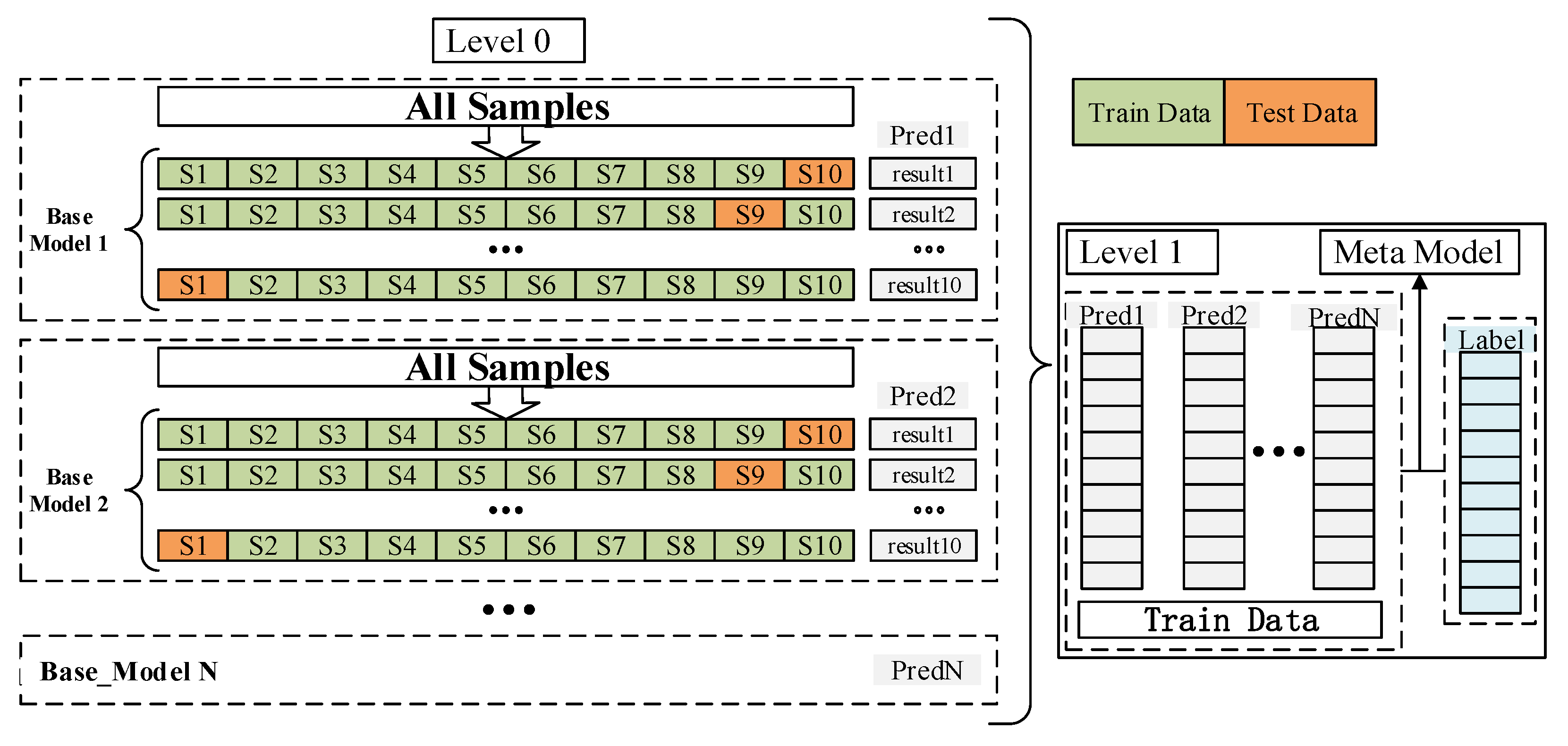
Stacked generalization (SG) is a layered ensemble algorithm [90]. Take two layers as an example. The first layer is called the base model, and its input is the original training set, which is trained using a k-fold crossover. The second layer is called the meta-model, and the output of the first layer is used as the training set for the retraining to obtain a complete stacking model [91]. In contrast to bagging and boosting, the base model in the SG method should be accurate and different. They can be bagging- and boosting-type algorithms, or KNN, SVR, and so on, but they have to have both less similarity and better estimation ability. The meta-model uses the estimation results of the base model as the input data for the training. The meta-model can be a single model or an ensemble model [39,92]. The construction process of the SG algorithm is shown in Figure 5. The optimal algorithm among the various algorithms was selected as the base model through model comparison, and different meta-models were chosen to construct the SG model.

Each algorithm has a different performance when using different parameters, and tuning the parameter is required to obtain the best estimation capability for each model. In the process of model tuning, root mean squared error (RMSE) was used as the evaluation metric of the model, and each set of parameters was evaluated using a grid search and repeated 10-fold CV. Finally, the set of parameters with the smallest RMSE was selected as the best combination of parameters for the model [93]. Table 4 lists the best parameter combinations for each machine learning algorithm. After tuning, we used 80% of the data in the entire dataset to train the model and used the other 20% of the data as the validation set to verify the estimation performance of the selected parameters. (In the experiment, we used scikit-learn to implement the required MLAs and the related processes based on Python 3.7.1 http://scikit-learn.org, (accessed on 31 May 2020)).

Table 4. Statistics of selected algorithms.

Methods	Name	Optimal Parameters	References
Bagging	Bagging Regressor (BAG)	max_samples = 1.0	[94]
		n_estimators = 100
	Random Forest (RF)	n_estimators = 425	[88,95]
		min_samples_split = 10
		min_samples_leaf = 10
Boosting	Ada Boost (ADA)	learning_rate = 0.03	[96]
		n_estimators = 225
	Cat boost (CBR)	Iterations = 575	[97]
		learning_rate = 0.02
	Gradient Boosting (GBR)	n_estimators = 650	[34]
		learning_rate = 0.1
	Light GBM (LGBM)	n_estimators = 815	[98]
		learning_rate = 0.12
	Extreme Gradient Boosting (XGBoost)	n_estimators = 620	[99,100]
		max_depth = 5
		learning_rate = 0.05
Stacking	Stacked Generalization(SG)	Depends on the base models	[33,101]
Linear	Linear Regression (LR)	Default	[102]
	Ridge	Default	[103]
	ElasticNet (ENe)	Default	[104]
	Lasso (LASSO)	Default	[105]
Neural Networks	Multi-layer perceptron (MLP)	solver = ‘adam’	[14,104]
		activation = ‘relu’
		hiden_layer_sizes = (100,100)
Tree-based	Decision Tree Regressor (DTR)	Default	[16,22,37]
	K-Neighbors Regression (KNN)	Default	[106]

Table 4. Statistics of selected algorithms.

Methods	Name	Optimal Parameters	References
Bagging	Bagging Regressor (BAG)	max_samples = 1.0	[94]
		n_estimators = 100
	Random Forest (RF)	n_estimators = 425	[88,95]
		min_samples_split = 10
		min_samples_leaf = 10
Boosting	Ada Boost (ADA)	learning_rate = 0.03	[96]
		n_estimators = 225
	Cat boost (CBR)	Iterations = 575	[97]
		learning_rate = 0.02
	Gradient Boosting (GBR)	n_estimators = 650	[34]
		learning_rate = 0.1
	Light GBM (LGBM)	n_estimators = 815	[98]
		learning_rate = 0.12
	Extreme Gradient Boosting (XGBoost)	n_estimators = 620	[99,100]
		max_depth = 5
		learning_rate = 0.05
Stacking	Stacked Generalization(SG)	Depends on the base models	[33,101]
Linear	Linear Regression (LR)	Default	[102]
	Ridge	Default	[103]
	ElasticNet (ENe)	Default	[104]
	Lasso (LASSO)	Default	[105]
Neural Networks	Multi-layer perceptron (MLP)	solver = ‘adam’	[14,104]
		activation = ‘relu’
		hiden_layer_sizes = (100,100)
Tree-based	Decision Tree Regressor (DTR)	Default	[16,22,37]
	K-Neighbors Regression (KNN)	Default	[106]

3.3. Evaluation Approaches

This study used three validation schemes to verify the model and experimental results: model-based cross-validation, validation based on independent samples, and comparative analysis with existing datasets.

• 10-fold cross-validation: After repeating the 10-fold cross-validation 5 times to ensure that all samples were tested, the RMSE, R², and MAE of each model were calculated, and their mean was calculated. The average value was used as an evaluation index of the algorithm’s accuracy [107].
• Independent validation:

  (a)

  When data were obtained in each reference area, 20% of each set of reference data was regarded as independent sample data (in Figure 6). When the model was trained, this part of the data does not participate in the training of the model. We used the trained model to predict this part of the data, compared the prediction results with the observed values of the sample, and used RMSE, R², and MAE as evaluation indicators to achieve the evaluation of the model’s predictive ability [108].

  (b)

  A reference region with a geographical location that differs from that in Section 2.2 is selected as the independent validation area, and this part of the data is used as the input data of the trained model for the prediction. The predicted results are compared with the observed value to verify the generalization ability of the model. This part of the validation data has better independence compared to the training and verification data in (a) have, because it is selected as an independent region and does not participate in the training and parameter optimization of the model.

• Product inter-comparison: We used the model for data production, and compared and verified the produced data with the Global Forest Change 2000–2019 (GFC) datasets and GLS_TCC datasets.

In this paper, the correlation coefficient (R² Equation (1)), mean absolute error (MAE, Equation (2)), and root mean square error (RMSE, Equation (3)) were selected as the evaluation indicators of the model’s performance [42,87,109].

$${\mathrm{R}}^2=1-\frac{{{\displaystyle \sum }}_i^n{\left(y_i-{\widehat{y}}_i\right)}^2}{{{\displaystyle \sum }}_i^n{\left(y_i-\overline{\mathrm{y}}\right)}^2}.$$

(1)

$$\mathrm{MAE}=\frac{1}{n}{{\displaystyle \sum }}_{i=1}^n\left|y_i-\widehat{y}\right|.$$

(2)

$$\mathrm{RMSE}=\sqrt{\frac{1}{n}{{\displaystyle \sum }}_{i=1}^n{\left(y_i-\widehat{y}\right)}^2}$$

(3)

In the equations $y_i, {\widehat{ y}}_i,$ and ${\overline{y}}_i$ are the original values, the prediction results, and the average value of the observations, respectively, and n is the number of observations.

4. Results Analysis

4.1. Comparing the Performance of Different ML Models

The performance and predictive ability of each model in Table 4 were statistically analyzed. The figures and tables in this section show the performance of each model. As summarized in the previous section, the DTR model is one of the most commonly used models and therefore we use the DTR model as a standard model to evaluate the performance of other models.

First, we evaluated all models using a 10-fold CV method repeated five times. The results are presented in

Table 5. 10-fold cross-validation results for all of the models.

Methods	Name	R2	MAE	RMSE
Bagging	BAG	0.992	0.020	0.035
	RF	0.993	0.020	0.033
Boosting	ADA	0.938	0.074	0.098
	CBR	0.991	0.025	0.038
	GBR	0.989	0.026	0.042
	LGBM	0.992	0.022	0.035
	XGBoost	0.989	0.026	0.041
Linear	LR	0.832	0.108	0.162
	Ridge	0.832	0.108	0.162
	ENe	0.759	0.130	0.194
	LASSO	0.768	0.130	0.191
NN	MLP	0.988	0.028	0.043
Tree-based	DTR	0.985	0.026	0.048
KNN	KNN	0.989	0.024	0.041

. The linear model was the worst type of all models, and ENe was the worst one of the linear models (R² = 0.759, MAE = 0.130, RMSE = 0.194); In the bagging ensemble, the RF model was the best performing model; in boosting ensemble, the LGBM model was the best performing model. The validation results of the RF were slightly better than those of the LGBM. The results of the MLP, DTR, and KNN were not very different.

We then used the validation dataset in Section 3.3 (2a) to evaluate the predictive ability of each model. The scatter plots of the predicted and observed values of each model are shown in Figure 7, where the red line represents the regression line of the predicted and observed values.

Table 6. Model estimation result statistics for independent datasets.

Methods	Name	R2	MAE	RMSE	Time(s)
Bagging	BAG	0.989	0.020	0.039	2640
	RF	0.991	0.019	0.035	6000
Boosting	ADA	0.952	0.068	0.093	440
	CBR	0.988	0.022	0.041	214
	GBR	0.989	0.021	0.040	2200
	LGBM	0.991	0.019	0.035	125
	XGBoost	0.989	0.021	0.038	342
Linear	LR	0.782	0.105	0.175	90
	Ridge	0.782	0.105	0.175	90
	ENe	0.649	0.139	0.224	100
	LASSO	0.674	0.136	0.217	110
NN	MLP	0.989	0.023	0.039	190
Tree-based	DTR	0.980	0.026	0.053	146
KNN	KNN	0.986	0.022	0.044	270

provides the statistics of the results in Figure 7. The scatter plot in Figure 7 shows that the scatter plots of ensemble models converged better, especially RF and LGBM. The worst performance was that of the linear model. Their scatter plots are more discrete and exhibit obvious overestimation of low-value areas.

Table 6 shows the estimation results of each model on independent datasets. In the bagging ensemble, the RF model was slightly better than BAG. In the boosting ensemble, the LGBM model performed the best, and its evaluation index was the same as that of the RF model (R² = 0.991, MAE = 0.019, RMSE = 0.035). Overall, the integrated models, except for the ADA model, showed better performance than the DTR. Comparing all algorithms, the R² of the linear regression algorithm was less than 0.8, the MAE was greater than 0.1, and the RMSE was greater than 0.17, the RMSE of the ENe model was more than 0.2, which was the worst performance among the linear models. It can be considered that linear models do not show the nonlinear relationship between FFC and features, so linear models are not suitable for use in this study. The MLP model was better than the linear models, and the evaluation index differed slightly from the DTR model. The KNN slightly outperformed the DTR model. Thus, the RF model and LGBM model in the ensemble algorithm performed better than other models in this study. The linear model was the worst-performing model, so it will not be mentioned in the discussion of the following experiments.

Considering that when building SG models, base models should have low correlation; that is, the types of base models should be different, and base models should have good performance. Based on the results of Table 6, the RF, DTR, LGBM, KNN, and MLP models were selected as base models. The choice of meta-model also affects the performance of the SG model. This study selected different meta-models to construct the SG algorithm model: SG(LGBM), SG(RF), SG(KNN), SG(DTR), and SG(MLP). (SG(RF) denotes the method using the RF algorithm as the meta-model).

Figure 8 shows the validation results of SG models in an independent dataset. The scatter plot of the SG(DTR) model is more discrete. For the SG model, although the same base models were selected, owing to the differences in meta-models, the performance of each SG model was different. According to the statistics in

Table 7. SG models estimation result.

Name	R2	MAE	RMSE	Time(s)
SG(DTR)	0.983	0.025	0.048	14,363
SG(KNN)	0.990	0.020	0.038	14,907
SG(LGBM)	0.991	0.018	0.034	9307
SG(MLP)	0.991	0.018	0.035	14,357
SG(RF)	0.991	0.019	0.036	19,998

, the SG(LGBM) model performed the best (R² = 0.991, MAE = 0.018, RMSE = 0.034). The RMSE of SG(MLP) was 0.001 higher than that of SG(LGBM). Thus, the two had the same performance. The worst performer was SG(DTR) (R² = 0.983, MAE = 0.025, RMSE = 0.048), which also indicates that the meta-model plays an important role in the performance of the entire model. According to the statistics in Table 6 and Table 7, SG(LGBM) is the best performer among all models.

4.2. Model Validation Based on Independent Validation Area

We used the validation data described in Section 3.3 (2b) to further verify the base model and the SG model. The validation data were taken from an independent area that does not participate in any process of the above models, so the data had better independence. The distribution of forests in these independent validation areas is quite different and was used to verify the performance of different models under different forest coverage conditions.

The scatter plots in Figure 9 are the estimated results of each model in the independent validation area.

Table 8. Statistics of the estimation results of each model in the independent validation areas.

	Area 1			Area 2			Area 3
	R2	MAE	RMSE	R2	MAE	RMSE	R2	MAE	RMSE
SG(DTR)	0.841	0.057	0.076	0.956	0.056	0.072	0.967	0.047	0.066
SG(KNN)	0.895	0.049	0.064	0.969	0.048	0.062	0.98	0.038	0.051
SG(LGBM)	0.911	0.048	0.061	0.971	0.043	0.056	0.984	0.034	0.046
SG(MLP)	0.907	0.047	0.06	0.973	0.043	0.056	0.983	0.035	0.048
SG(RF)	0.910	0.048	0.062	0.97	0.043	0.056	0.982	0.036	0.048
DTR	0.85	0.057	0.076	0.924	0.066	0.085	0.965	0.048	0.067
KNN	0.859	0.042	0.064	0.972	0.05	0.066	0.975	0.043	0.059
LGBM	0.911	0.046	0.059	0.972	0.047	0.061	0.982	0.038	0.048
MLP	0.903	0.038	0.055	0.973	0.043	0.056	0.983	0.037	0.049
RF	0.889	0.049	0.065	0.975	0.04	0.052	0.983	0.036	0.048

presents the statistics of the estimation accuracy of the model in the three validation areas. In area 1, the models with the highest R² were LGBM and SG(LGBM) (R² = 0.911). The MLP model had the best MAE (0.038) and RMSE (0.055). In the stacking algorithm, SG(MLP) had the best MAE (0.047) and RMSE (0.060). It can be considered that SG(MLP) was the best stacking model in this area. Although the R² of MLP was lower than LGBM, it had better MAE and RMSE, so MLP was the best base model in this area, but also the best model compared to all models. The data distribution in area 2 was opposite to that in area 1, and the data were mainly distributed in high value. RF was the best base model, SG(MLP) was the best-stacked model. In area 3, the SG(LGBM) model had the best R², MAE, and RMSE (0.984, 0.034, 0.046). In the base model, the RF model has the best R², MAE, and RMSE (0.983, 0.036, 0.048). The findings from the above analysis indicate that the SG(LGBM) model is an ensemble model with better performance, and the RF model is a base model with better overall performance.

We divided the data of all validation areas into five layers according to the interval of 0–0.2, 0.2–0.4, 0.4–0.6, 0.6–0.8, and 0.8–1. Based on the findings above, firstly, the RF model is the best base model and the SG(LGBM) is the best-integrated model. Considering that the SG(MLP) model and the SG(LGBM) model are less different. The DTR model, as one of the most used models, can be used as a standard model, so the DTR, RF, SG(LGBM), and SG(MLP) models were chosen for comparative analysis.

Table 9. Performance statistics of models for stratified data.

FFC Strata		0–0.2	0.2–0.4	0.4–0.6	0.6–0.8	0.8–1	0–1
n_Points		51,218	2603	2362	5094	30,728	92,005
R2	DTR	0.462	0.247	0.138	0.218	0.035	0.965
	RF	0.616	0.377	0.329	0.457	0.161	0.987
	SG(LGBM)	0.623	0.411	0.351	0.504	0.175	0.988
	SG(MLP)	0.634	0.388	0.362	0.539	0.199	0.989
MAE	DTR	0.017	0.086	0.091	0.101	0.067	0.042
	RF	0.013	0.064	0.065	0.082	0.04	0.029
	SG(LGBM)	0.013	0.061	0.064	0.076	0.041	0.028
	SG(MLP)	0.012	0.063	0.063	0.077	0.041	0.028
RMSE	DTR	0.039	0.11	0.127	0.157	0.094	0.077
	RF	0.028	0.079	0.086	0.106	0.055	0.049
	SG(LGBM)	0.028	0.076	0.084	0.093	0.054	0.047
	SG(MLP)	0.028	0.078	0.083	0.092	0.052	0.046

shows the estimation results for the four models. The scatterplot in Figure 10 shows the performance of the RF model for estimating the stratified data. Figure 10a–e shows the estimation results for the stratified data for different intervals and Figure 10f shows the performance of the model for the whole data. the R² for the stratified data is very limited due to the scattering pattern along the short distances. Figure 11a,c,e are histograms of the evaluation indicators of the three models at different levels. When the coverage was less than 0.2, the highest R² was the SG(MLP) model (R² = 0.634), and the DTR model performed the worst; when the coverage is 0.2–0.4, SG(LGBM) performed best (R² = 0.411, MAE = 0.061, RMSE = 0.076); when the coverage was 0.6–1, SG(MLP) was the best model. The overall result elicited the same conclusion: The estimation result of the integrated algorithm in the independent validation area is significantly improved compared with the base model, especially for the non-ensemble model.

Figure 11 b,d,f show the differences between the R², MAE, and RMSE values of the layered verification and overall verification: R² had the largest variation range when the coverage was greater than 0.8, and the variation range of MAE and RMSE when the coverage was 0.2–0.8 is significantly higher than other coverage intervals. The DTR model had the largest change in all stratified intervals, and the MAE and RMSE of the SG(LGBM) model had the smallest changes when the coverage was 0.2–0.4 and 0.6–0.8. According to the histogram in Figure 11, all models performed poorly when the coverage was between 0.2 and 0.8, in particular, the MAE and RMSE metrics were greatest for all models at coverage levels of 0.6–0.8, which would suggest that the models had the worst performance at this coverage condition. This is because when the coverage was 0.6–0.8, the surface heterogeneity was greater than other coverages. Whether in sample acquisition or model prediction, the similarity between different samples in the obviously heterogeneous mixed region was greater, which caused errors in the training or prediction of the model and affected the final estimation ability of the model.

Based on the comprehensive performance of all models, SG(LGBM) and SG(MLP) model performance were slightly higher than the RF, and much higher than that of the DTR model, indicating that the stacking method is better than some base models such as the DTR model, but some base model (RF) has comparable results to stacking method. As the model constructed by the SG method is a superposition of multiple base models, it requires longer computing time and computing resources. Table 6 and Table 7 list the time required for each model.

4.3. Comparison with Existing Products

The performance of the SG algorithm was improved compared to the base model, but the SG algorithm requires a longer calculation time and consumes more calculation resources during its operation. Therefore, based on the consideration of the calculation efficiency and estimation accuracy, in this section, the RF model was selected as the estimation model to estimate the FFC, and the estimated FFC was compared and verified with other datasets. Figure 12 shows the distribution of forests in the TNR of different datasets, including the FromGLC2017 dataset (Figure 12a), GLS_TCC (2015) dataset (Figure 12b), GFC dataset (Figure 12c), and the FFC2017 dataset estimated by this model (Figure 12d). From an intuitive point of view, the four figures all show the main distribution regularities of the TNR forests. The forests are mainly distributed in the northeastern region, the central region has a slightly lower distribution, and the northwestern region has the sparsest distribution. However, there are differences in the spatial distribution of forests in these figures. The area covered by forests in Figure 11b,d is more extensive than in Figure 11a,c, especially the forests with a low cover density, and the forest cover in Figure 12c is more consistent with the spatial distribution in Figure 12a.

We selected six areas as the validation dataset to compare and analyze the FFC, GFC, and GLS_TCC. Figure 13 shows the comparison results.

Figure 13 shows the results of the comparison among the datasets, Figure 13a shows the result of aggregating the GF-2 forest distribution maps with a 1-m resolution into 30-m resolution, which we call GF2AG30. The aggregated data are completely independent throughout the experiment and can be used as true data. In the visual comparison, compared with GLS_TCC and GFC, FFC has a better spatial distribution consistency with GF2AG30. In areas (1) and (2), FFC contains more forest distribution details than GFC and GLS_TCC, especially at the junctions of the forest and non-forest areas where the changing trend of the forest density can be seen. Compared with GF2AG30 (Figure 13a) for each area, in the non-forest areas, GLS_TCC is overestimated. For example, the white in Figure 13(1a) indicates the value of 0, which means that there is no forest cover, but the corresponding Figure 13(1c) indicates that there is forest cover. In the forest-covered areas, GFC is underestimated. The distributions of the forests in areas (5) and (6) are discrete, but the results of GFC show that there is basically no forest cover in these two areas. Figure 13e shows a stacked histogram of the frequency distributions of the four datasets for each area, which illustrates the differences in the frequencies and distribution ranges of the datasets. In general, the ranges of the four datasets have obvious differences. First, the value range of GF2AG30, FFC, and GFC is 0–100%, but GLS_TCC basically does not have a pixel value of greater than 80%. In forest-covered areas 1 and 2, the data distributions of GF2AG30, FFC, and GFC are relatively consistent; while in GLS_TCC, the forest coverage in these two areas is concentrated between 50% and 60%. In areas 3 and 4, GLS_TCC is concentrated at about 50%; while GFC is concentrated at about 40% in area 3 and at about 60% in area 4. Compared with GF2AG30, GLS_TCC and GFC are underestimated. The forest distribution of FFC is more consistent with that of GF2AG30 than in GLS_TCC and GFC. The land cover in areas 5 and 6 is dominated by non-forest vegetation, and the forests are scattered. GF2AG30 and FFC show the characteristics of the forest distribution better, while GLS_TCC exhibits overestimation in the low-value areas and underestimation in the high-value areas. In Figure 13f–h are the scatter density plots of the correlations between FFC and GF2AG30, GLS_TCC and GF2AG30, and GFC and GF2AG30, respectively. Overall, FFC has the highest correlation with GF2AG30, followed by GLS_TCC and GF2AG30, and GF2AG30 has the worst correlation with GFC.

5. Discussion

5.1. Algorithmic Factors

In this study, we used a combination of Landsat and GF-2 RS images to evaluate the applicability, stability, and generalization ability of several MLAs at estimating the FFC. In this study, a variety of SG models were constructed, and the results show that the SG models with different meta-models have different performances, among which the SG(LGBM) and SG(MLP) models achieved the best-estimated results and the estimation accuracy was improved compared to the base model (DTR). Since the SG model is based on the fusion of multiple MLAs, its computational efficiency is related to the selection of the base model and meta-model. The more base-model or more complex meta-model is selected, the more computational resources are required and the longer the computation time. Some studies have demonstrated the advantages of integrated models over base models [33,110], but Wen and Hughes [39] concluded that although integrated models have high predictive power, some of their metrics are inferior to the RF models. The SG model developed in this paper is significantly better than a base model such as the DTR, but it has a limited accuracy improvement compared to the integrated type of RF. To obtain the obvious advantages of the SG method, further research and discussion of the applicability of the SG model and the selection of base models are needed.

5.2. Time Factors

Relevant studies have demonstrated that using continuous fractions instead of classification classes can enhance the assessment of the forest status and its changes [20,21,28]. In addition, the quality of the samples is related to the performance of the model and the accuracy of the parameter estimation, while the temporal consistency between the reference image and the image to be estimated affects the quality of the sample. In this study, Landsat and GF-2 remote sensing images with small differences in imaging time were selected to ensure the consistency of the extracted information. However, the differences in the revisit periods of the two satellite sensors and the influence of the weather factors, and the amount of time-consistent image data were small. The study area contains a variety of forest types, and different types of forests behave differently on remote sensing images with seasonal changes, especially deciduous broadleaf forests that change significantly with the season [20]. The RS data selected in this study were mostly obtained in the forest growing season, which may limit the time range of the model’s usage due to the lack of samples from other seasons [18,20]. Therefore, in future research, it will be necessary to consider the combined use of multi-source data to increase the representativeness of the sample and to explore the effects of different forest types and tree species on the estimation of forest coverage under seasonal changes.

5.3. Sample Representativeness Factor

One of the key challenges in estimating forest attributes such as FFC using medium spatial resolution satellite imagery is the difficulty in overcoming background soil reflectance, especially in low-density sparse forests [57]. The entire study area contains a large amount of non-forest vegetation and low-density woodlands, which are prone to higher errors if the information is not sufficiently representative [18,20]. We increased the proportion of low-value samples in the entire dataset to improve the representativeness of the samples. However, the inclusion of too much low-value data tends to cause an unbalanced distribution of samples and leads to more errors in the model estimation. In this study, a 5 × 5 sampling window was used to reduce the effect of the spatial misregistration between the Landsat and GF-2 data. It is easy to generate samples with errors in sparse woodlands or forest boundaries, and such errors have a negative impact on the training and application of the model. Therefore, to ensure the representativeness of the data, our future work will pay more attention to the extraction and analysis of low-density forest information and improve the accuracy of sample extraction.

5.4. Differences between Data Products

The comparison between the FFC, GFC, and GLS_TCC datasets shows that there are large differences between them, and the differences are due to several reasons:

Source data differences: The GLS_TCC dataset is an annual composite. For example, the 2005 GLS_TCC is a composite of Landsat-5 and Landsat-7 images from 2003 to 2008 [21,111]. Similarly, the GFC is an annual synthesized data product. In contrast, the validation data in this paper are time-determined images, which can be considered to be instantaneous data from the image at the moment of imaging. Inconsistency in the timing of the data may be a reason for the discrepancy between the different products.

Differences in sample data: Both the GLS_TCC and GFC refer to the MOD44B_VCF data product when selecting the samples and constructing the models, and inevitably, they inherit the uncertainty that exists in the product itself [21]. The use of the 250 m resolution MOD44BVCF limits the ability to acquire canopy cover values below 30 m [21,112], while the reference data of the FFC is a higher resolution remote sensing image with a stronger ability to acquire fine canopy cover data.

Algorithm differences: The GLS_TCC uses the standard regression tree (RT) algorithm, and the GFC uses the decision regression tree (RT) method. In this study, several algorithms were compared and it was concluded that the DT algorithm is computationally efficient, but its estimation accuracy and ability to prevent overfitting are not as good as those of the ensemble method. In this study, ensemble learning methods such as the RF were chosen. Although the computational efficiency is not as good as that of the DT, which has a better model generalization ability and estimation performance [83,113].

6. Conclusions

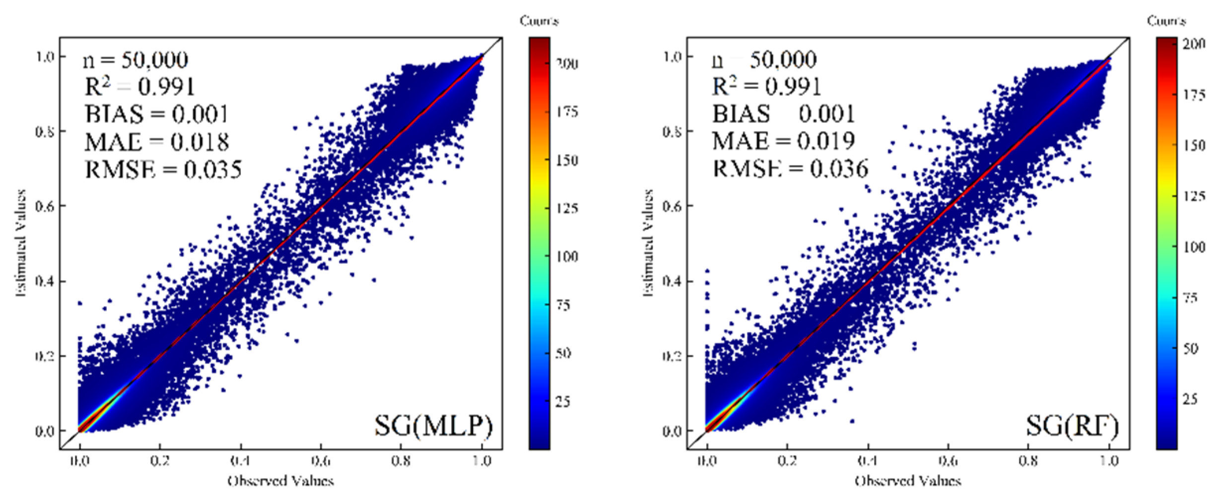
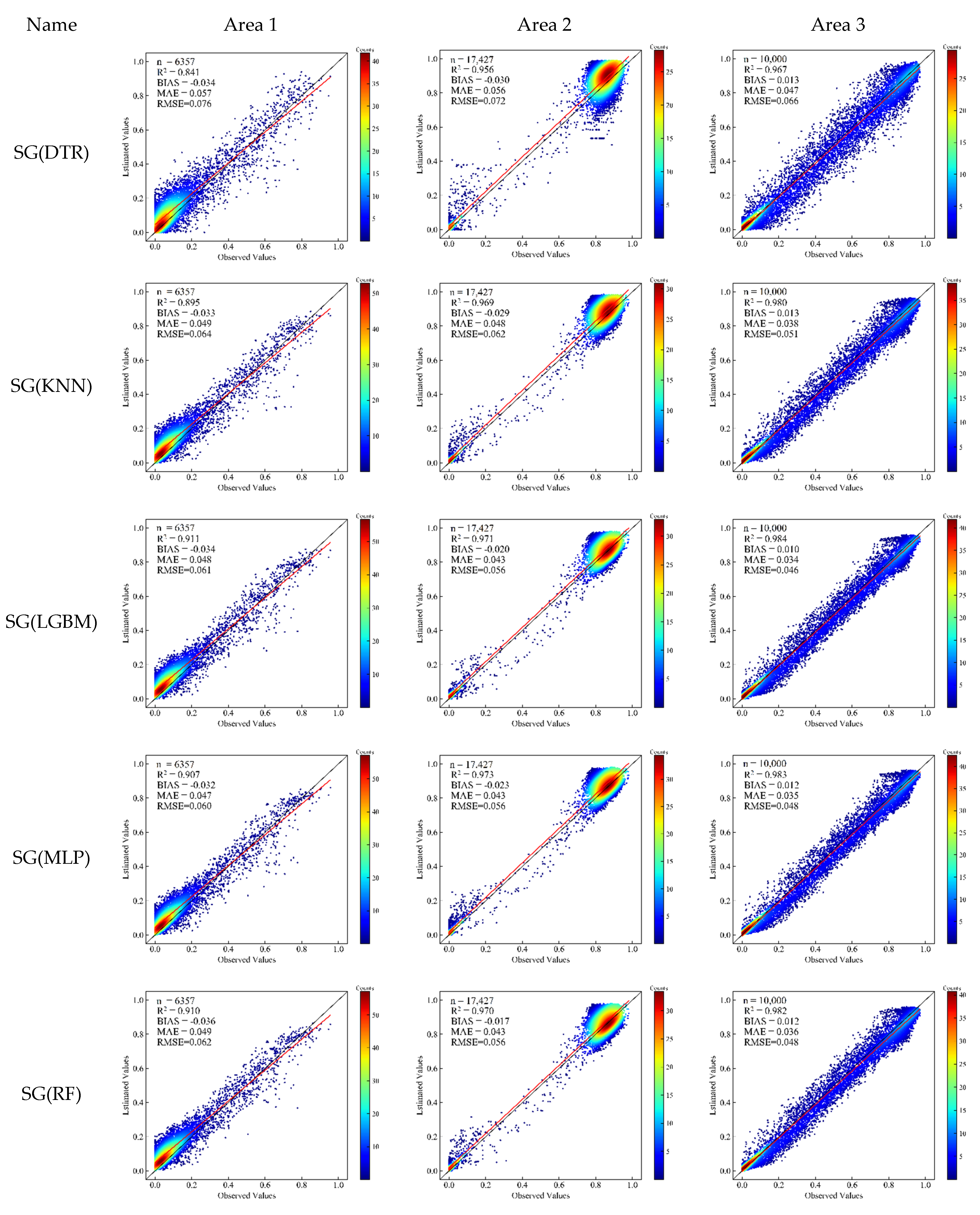
This study aimed to estimate the 30-m resolution FFC in the TNR of China. Landsat RS images were used to obtain band information and the vegetation index, GF-2 RS images were used as reference image data to obtain forest coverage information in the study area combined with auxiliary topographic factors, and machine learning methods were used to construct a method for estimating forest coverage in China’s TNR model. The results of the cross-validation and independent validation indicate that simple linear models cannot accurately represent the relationships between features and the FFC. The performance of ensemble models was better than that of other types of models, and RF (R² = 0.991, MAE = 0.019, RMSE = 0.035) and LGBM (R² = 0.991, MAE = 0.019, RMSE = 0.035) were the best of bagging ensemble models and boosting ensemble models, respectively. In this study, five models (RF, LGBM, MLP, DTR, KNN) with lower correlations but better performances were selected as the base models, and multiple SG algorithms were constructed using different meta-models. The results show that the selection of the meta-model is one factor that affects the performance of the SG algorithms. Moreover, the best SG model SG(LGBM) (R² = 0.991, MAE = 0.018, RMSE = 0.034) had a better performance than the DTR (R² = 0.980, MAE = 0.026, RMSE = 0.053). The results of stratification statistics indicate that when the coverage is below 0.2 and the coverages are above 0.8. The model has better performance, but the estimation ability of the model decreases between the coverages of 0.2 and 0.8. There are two possible reasons for this: (1) the number of samples in the range of 0.2 to 0.8 is small during the model training and model validation, so the model’s estimation ability in this range is weak; (2) Because the forest is not completely closed within the 0.2–0.8 cover range, the surface coverage is complex and the heterogeneity is high, which also indicates that further research is needed for areas with high surface heterogeneity. Through the comparative analysis of the dataset in the independent validation area, the GLS_TCC data were underestimated in the validation area, and the GFC data were underestimated in the high-value area, and through comparison with the forest aggregation map of the validation area, the forest distribution of the FFC had better consistency with the reference data and showed more detailed forest distribution trends. In addition, we also need to implement a more accurate validation of the estimated FFC and compare it with previous studies and data, as well as a more detailed study of the FFC for regions with a high surface heterogeneity.

References

1. Liang, S.; Wang, J. Advanced Remote Sensing: Terrestrial Information Extraction and Applications, 2nd ed.; Academic Press/Elsevier: Cambridge, UK, 2019; p. 1010. [Google Scholar]
2. Liang, S. Quantitative Remote Sensing of Land Surfaces; John Wiley & Sons, Inc.: New York, NY, USA, 2004. [Google Scholar]
3. Pugh, T.A.M.; Arneth, A.; Kautz, M.; Poulter, B.; Smith, B. Important role of forest disturbances in the global biomass turnover and carbon sinks. Nat. Geosci. 2019, 12, 730–735. [Google Scholar] [CrossRef] [PubMed]
4. Martin, A.R.; Doraisami, M.; Thomas, S.C. Global patterns in wood carbon concentration across the world’s trees and forests. Nat. Geosci. 2018, 11, 915–920. [Google Scholar] [CrossRef]
5. Crowther, T.W.; Glick, H.B.; Covey, K.R.; Bettigole, C.; Maynard, D.S.; Thomas, S.M.; Smith, J.R.; Hintler, G.; Duguid, M.C.; Amatulli, G.; et al. Mapping tree density at a global scale. Nature 2015, 525, 201–205. [Google Scholar] [CrossRef] [PubMed]
6. Srivastava, A.; Sahoo, B.; Raghuwanshi, N.S.; Singh, R. Evaluation of Variable-Infiltration Capacity Model and MODIS-Terra Satellite-Derived Grid-Scale Evapotranspiration Estimates in a River Basin with Tropical Monsoon-Type Climatology. J. Irrig. Drain. Eng. 2017, 143, 04017028. [Google Scholar] [CrossRef] [Green Version]
7. Elbeltagi, A.; Aslam, M.R.; Malik, A.; Mehdinejadiani, B.; Srivastava, A.; Bhatia, A.S.; Deng, J. The impact of climate changes on the water footprint of wheat and maize production in the Nile Delta, Egypt. Sci. Total Environ. 2020, 743, 140770. [Google Scholar] [CrossRef] [PubMed]
8. Suo, X.; Cao, S. China’s three north shelter forest program: Cost–benefit analysis and policy implications. Environ. Dev. Sustain. 2021, 1–14. [Google Scholar] [CrossRef]
9. Peng, D.; Wu, C.; Zhang, B.; Huete, A.; Zhang, X.; Sun, R.; Lei, L.; Huang, W.; Liu, L.; Liu, X.; et al. The Influences of Drought and Land-Cover Conversion on Inter-Annual Variation of NPP in the Three-North Shelterbelt Program Zone of China Based on MODIS Data. PLoS ONE 2016, 11, e0158173. [Google Scholar] [CrossRef]
10. Deng, C.; Zhang, B.; Cheng, L.; Hu, L.; Chen, F. Vegetation dynamics and their effects on surface water-energy balance over the Three-North Region of China. Agric. For. Meteorol. 2019, 275, 79–90. [Google Scholar] [CrossRef]
11. Cao, S.; Suo, X.; Xia, C. Payoff from afforestation under the Three-North Shelter Forest Program. J. Clean. Prod. 2020, 256, 120461. [Google Scholar] [CrossRef]
12. Chu, X.; Zhan, J.; Li, Z.; Zhang, F.; Qi, W. Assessment on forest carbon sequestration in the Three-North Shelterbelt Program region, China. J. Clean. Prod. 2019, 215, 382–389. [Google Scholar] [CrossRef]
13. Huang, T.; Zhang, X.; Ling, Z.; Zhang, L.; Gao, H.; Tian, C.; Guo, J.; Zhao, Y.; Wang, L.; Ma, J. Impacts of Large-Scale Land-Use Change on the Uptake of Polycyclic Aromatic Hydrocarbons in the Artificial Three Northern Regions Shelter Forest Across Northern China. Environ. Sci. Technol. 2016, 50, 12885–12893. [Google Scholar] [CrossRef] [Green Version]
14. Jia, K.; Liang, S.; Xiangqin, W.; Li, Q.; Du, X.; Jiang, B.; Yao, Y.; Zhao, X.; Li, Y. Fractional Forest Cover Changes in Northeast China From 1982 to 2011 and Its RelationshipWith Climatic Variations. IEEE Trans. Geosci. Remote Sens. 2015, 8, 775–783. [Google Scholar]
15. Mayes, M.T.; Mustard, J.F.; Melillo, J.M. Forest cover change in Miombo Woodlands: Modeling land cover of African dry tropical forests with linear spectral mixture analysis. Remote Sens. Environ. 2015, 165, 203–215. [Google Scholar] [CrossRef]
16. Hansen, M.C.; DeFries, R.S.; Townshend, J.R.G.; Carroll, M.; Dimiceli, C.; Sohlberg, R.A. Global Percent Tree Cover at a Spatial Resolution of 500 Meters: First Results of the MODIS Vegetation Continuous Fields Algorithm. Earth Interact. 2003, 7, 1–15. [Google Scholar] [CrossRef] [Green Version]
17. Pouliot, D.; Latifovic, R.; Zabcic, N.; Guindon, L.; Olthof, I. Development and assessment of a 250m spatial resolution MODIS annual land cover time series (2000–2011) for the forest region of Canada derived from change-based updating. Remote Sens. Environ. 2014, 140, 731–743. [Google Scholar] [CrossRef]
18. Zhu, X.; Liu, D. Improving forest aboveground biomass estimation using seasonal Landsat NDVI time-series. ISPRS J. Photogramm. Remote Sens. 2015, 102, 222–231. [Google Scholar] [CrossRef]
19. Hansen, M.C.; Loveland, T.R. A review of large area monitoring of land cover change using Landsat data. Remote Sens. Environ. 2012, 122, 66–74. [Google Scholar] [CrossRef]
20. Senf, C.; Laštovička, J.; Okujeni, A.; Heurich, M.; van der Linden, S. A generalized regression-based unmixing model for mapping forest cover fractions throughout three decades of Landsat data. Remote Sens. Environ. 2020, 240, 111691. [Google Scholar] [CrossRef]
21. Sexton, J.O.; Song, X.-P.; Feng, M.; Noojipady, P.; Anand, A.; Huang, C.; Kim, D.-H.; Collins, K.M.; Channan, S.; DiMiceli, C.; et al. Global, 30-m resolution continuous fields of tree cover: Landsat-based rescaling of MODIS vegetation continuous fields with lidar-based estimates of error. Int. J. Digit. Earth 2013, 6, 427–448. [Google Scholar] [CrossRef] [Green Version]
22. Gessner, U.; Machwitz, M.; Conrad, C.; Dech, S. Estimating the fractional cover of growth forms and bare surface in savannas. A multi-resolution approach based on regression tree ensembles. Remote Sens. Environ. 2013, 129, 90–102. [Google Scholar] [CrossRef] [Green Version]
23. Baumann, M.; Levers, C.; Macchi, L.; Bluhm, H.; Waske, B.; Gasparri, N.I.; Kuemmerle, T. Mapping continuous fields of tree and shrub cover across the Gran Chaco using Landsat 8 and Sentinel-1 data. Remote Sens. Environ. 2018, 216, 201–211. [Google Scholar] [CrossRef]
24. Mahdavi, A.; Aziz, J. Estimation of Semiarid Forest Canopy Cover Using Optimal Field Sampling and Satellite Data with Machine Learning Algorithms. J. Indian Soc. Remote Sens. 2020, 48, 575–583. [Google Scholar] [CrossRef]
25. Jennings, S.; Brown, N.; Sheil, D. Assessing forest canopies and understorey illumination: Canopy closure, canopy cover and other measures. For. Int. J. For. Res. 1999, 72, 59–74. [Google Scholar] [CrossRef]
26. McIntosh, A.C.S.; Gray, A.N.; Garman, S.L. Estimating Canopy Cover from Standard Forest Inventory Measurements in Western Oregon. For. Sci. 2012, 58, 154–167. [Google Scholar] [CrossRef] [Green Version]
27. Rokhmatuloh; Nitto, D.; Bilbisi, H.A.; Arihara, K.; Tateishi, R. Estimating Percent Tree Cover Using Regression Tree Method with Very-High-Resolution QuickBird Images as Training Data. J. Remote Sens. Soc. Jpn. 2007, 1, 1–12. [Google Scholar]
28. Hansen, M.C.; Potapov, P.V.; Moore, R.; Hancher, M.; Turubanova, S.A.; Tyukavina, A.; Thau, D.; Stehman, S.V.; Goetz, S.J.; Loveland, T.R.; et al. High-Resolution Global Maps of 21st-Century Forest Cover Change. Science 2013, 342, 850–853. [Google Scholar] [CrossRef] [Green Version]
29. Townshend, J.R.G.; Hansen, M.C.; Carroll, M.; DiMiceli, C.; Sohlberg, R.; Huang, C. Vegetation Continuous Fields MOD44B, 2010 Percent Tree Cover; University of Maryland: College Park, MD, USA, 2011. [Google Scholar]
30. Qiu, B.; Chen, G.; Tang, Z.; Lu, D.; Wang, Z.; Chen, C. Assessing the Three-North Shelter Forest Program in China by a novel framework for characterizing vegetation changes. ISPRS J. Photogramm. Remote Sens. 2017, 133, 75–88. [Google Scholar] [CrossRef]
31. Yang, Y.; Xiao, P.; Feng, X.; Li, H. Accuracy assessment of seven global land cover datasets over China. ISPRS J. Photogramm. Remote Sens. 2017, 125, 156–173. [Google Scholar] [CrossRef]
32. Jia, T.; Li, Y.; Shi, W.; Zhu, L. Deriving a Forest Cover Map in Kyrgyzstan Using a Hybrid Fusion Strategy. Remote Sens. 2019, 11, 2325. [Google Scholar] [CrossRef] [Green Version]
33. Healey, S.P.; Cohen, W.B.; Yang, Z.; Kenneth Brewer, C.; Brooks, E.B.; Gorelick, N.; Hernandez, A.J.; Huang, C.; Joseph Hughes, M.; Kennedy, R.E.; et al. Mapping forest change using stacked generalization: An ensemble approach. Remote Sens. Environ. 2018, 204, 717–728. [Google Scholar] [CrossRef]
34. Godinho, S.; Guiomar, N.; Gil, A. Estimating tree canopy cover percentage in a mediterranean silvopastoral systems using Sentinel-2A imagery and the stochastic gradient boosting algorithm. Int. J. Remote Sens. 2018, 39, 4640–4662. [Google Scholar] [CrossRef]
35. Egorov, A.; Roy, D.; Zhang, H.; Hansen, M.; Kommareddy, A. Demonstration of Percent Tree Cover Mapping Using Landsat Analysis Ready Data (ARD) and Sensitivity with Respect to Landsat ARD Processing Level. Remote Sens. 2018, 10, 209. [Google Scholar] [CrossRef] [Green Version]
36. Donmez, C.; Berberoglu, S.; Erdogan, M.A.; Tanriover, A.A.; Cilek, A. Response of the regression tree model to high resolution remote sensing data for predicting percent tree cover in a Mediterranean ecosystem. Environ. Monit. Assess. 2015, 187, 4. [Google Scholar] [CrossRef]
37. Selkowitz, D.J. A comparison of multi-spectral, multi-angular, and multi-temporal remote sensing datasets for fractional shrub canopy mapping in Arctic Alaska. Remote Sens. Environ. 2010, 114, 1338–1352. [Google Scholar] [CrossRef]
38. Graczyk, M.; Lasota, T.; Trawiński, B.; Trawiński, K. Comparison of Bagging, Boosting and Stacking Ensembles Applied to Real Estate Appraisal. Lect. Notes Comput. Sci. 2010, 5991, 340–350. [Google Scholar]
39. Wen, L.; Hughes, M. Coastal wetland mapping using ensemble learning algorithms: A comparative study of bagging, boosting and stacking techniques. Remote Sens. 2020, 12, 1683. [Google Scholar] [CrossRef]
40. Carter, C.; Liang, S. Evaluation of ten machine learning methods for estimating terrestrial evapotranspiration from remote sensing. Int. J. Appl. Earth Obs. Geoinf. 2019, 78, 86–92. [Google Scholar] [CrossRef]
41. Wu, Y.; Duguay, C.R.; Xu, L. Assessment of machine learning classifiers for global lake ice cover mapping from MODIS TOA reflectance data. Remote Sens. Environ. 2021, 253. [Google Scholar] [CrossRef]
42. Elbeltagi, A.; Kumari, N.; Dharpure, J.K.; Mokhtar, A.; Alsafadi, K.; Kumar, M.; Mehdinejadiani, B.; Ramezani Etedali, H.; Brouziyne, Y.; Towfiqul Islam, A.R.M.; et al. Prediction of Combined Terrestrial Evapotranspiration Index (CTEI) over Large River Basin Based on Machine Learning Approaches. Water 2021, 13, 547. [Google Scholar] [CrossRef]
43. Shiferaw, H.; Bewket, W.; Eckert, S. Performances of machine learning algorithms for mapping fractional cover of an invasive plant species in a dryland ecosystem. Ecol. Evol. 2019, 9, 2562–2574. [Google Scholar] [CrossRef] [Green Version]
44. Halperin, J.; LeMay, V.; Coops, N.; Verchot, L.; Marshall, P.; Lochhead, K. Canopy cover estimation in miombo woodlands of Zambia: Comparison of Landsat 8 OLI versus RapidEye imagery using parametric, nonparametric, and semiparametric methods. Remote Sens. Environ. 2016, 179, 170–182. [Google Scholar] [CrossRef]
45. Korhonen, L.; Hadi; Packalen, P.; Rautiainen, M. Comparison of Sentinel-2 and Landsat 8 in the estimation of boreal forest canopy cover and leaf area index. Remote Sens. Environ. 2017, 195, 259–274. [Google Scholar] [CrossRef]
46. Narine, L.L.; Popescu, S.; Neuenschwander, A.; Zhou, T.; Srinivasan, S.; Harbeck, K. Estimating aboveground biomass and forest canopy cover with simulated ICESat-2 data. Remote Sens. Environ. 2019, 224, 1–11. [Google Scholar] [CrossRef]
47. Sunde, M.G.; Diamond, D.D.; Elliott, L.F.; Hanberry, P.; True, D. Mapping high-resolution percentage canopy cover using a multi-sensor approach. Remote Sens. Environ. 2020, 242, 111748. [Google Scholar] [CrossRef]
48. Tsai, Y.H.; Stow, D.; Shi, L.; Lewison, R.; An, L. Quantifying canopy fractional cover and change in Fanjingshan National Nature Reserve, China using multi-temporal Landsat imagery. Remote Sens. Lett. 2016, 7, 671–680. [Google Scholar] [CrossRef]
49. Pengra, B.; Long, J.; Dahal, D.; Stehman, S.V.; Loveland, T.R. A global reference database from very high resolution commercial satellite data and methodology for application to Landsat derived 30 m continuous field tree cover data. Remote Sens. Environ. 2015, 165, 234–248. [Google Scholar] [CrossRef]
50. Wu, Q.; Zhong, R.; Zhao, W.; Song, K.; Du, L. Land-cover classification using GF-2 images and airborne lidar data based on Random Forest. Int. J. Remote Sens. 2018, 40, 2410–2426. [Google Scholar] [CrossRef]
51. Zhou, J.; Dian, Y.; Wang, X.; Yao, C.; Jian, Y.; Li, Y.; Han, Z. Comparison of GF2 and SPOT6 Imagery on Canopy Cover Estimating in Northern Subtropics Forest in China. Forests 2020, 11, 407. [Google Scholar] [CrossRef] [Green Version]
52. Sun, S.; Li, Z.; Tian, X.; Gao, Z.; Wang, C.; Gu, C. Forest Canopy Closure Estimation in Greater Khingan Forest Based on Gf-2 Data. In Proceedings of the IGARSS 2019—2019 IEEE International Geoscience and Remote Sensing Symposium, Yokohama, Japan, 28 July–2 August 2019; pp. 6640–6643. [Google Scholar]
53. Jia, K.; Liang, S.L.; Liu, J.Y.; Li, Q.Z.; Wei, X.Q.; Yuan, W.P.; Yao, Y.J. Forest Cover Changes in the Three-North Shelter Forest Region of China during 1990 to 2005. J. Environ. Inform. 2015, 26. [Google Scholar] [CrossRef]
54. Xie, X.; Liang, S.; Yao, Y.; Jia, K.; Meng, S.; Li, J. Detection and attribution of changes in hydrological cycle over the Three-North region of China: Climate change versus afforestation effect. Agric. For. Meteorol. 2015, 203, 74–87. [Google Scholar] [CrossRef]
55. Yao, Y.; Xie, X.; Meng, S.; Zhu, B.; Zhang, K.; Wang, Y. Extended Dependence of the Hydrological Regime on the Land Cover Change in the Three-North Region of China: An Evaluation under Future Climate Conditions. Remote Sens. 2019, 11, 81. [Google Scholar] [CrossRef] [Green Version]
56. Friedl, M.A.; Sulla-Menashe, D.; Tan, B.; Schneider, A.; Ramankutty, N.; Sibley, A.; Huang, X. MODIS Collection 5 global land cover: Algorithm refinements and characterization of new datasets. Remote Sens. Environ. 2010, 114, 168–182. [Google Scholar] [CrossRef]
57. Safari, A.; Sohrabi, H.; Powell, S.; Shataee, S. A comparative assessment of multi-temporal Landsat 8 and machine learning algorithms for estimating aboveground carbon stock in coppice oak forests. Int. J. Remote Sens. 2017, 38, 6407–6432. [Google Scholar] [CrossRef]
58. Wang, J.; Xiao, X.; Bajgain, R.; Starks, P.; Steiner, J.; Doughty, R.B.; Chang, Q. Estimating leaf area index and aboveground biomass of grazing pastures using Sentinel-1, Sentinel-2 and Landsat images. ISPRS J. Photogramm. Remote Sens. 2019, 154, 189–201. [Google Scholar] [CrossRef] [Green Version]
59. Zhu, Z.; Woodcock, C.E.; Holden, C.; Yang, Z. Generating synthetic Landsat images based on all available Landsat data: Predicting Landsat surface reflectance at any given time. Remote Sens. Environ. 2015, 162, 67–83. [Google Scholar] [CrossRef]
60. Zhu, Z.; Woodcock, C.E.; Olofsson, P. Continuous monitoring of forest disturbance using all available Landsat imagery. Remote Sens. Environ. 2012, 122, 75–91. [Google Scholar] [CrossRef]
61. Landry, S.; St-Laurent, M.-H.; Nelson, P.R.; Pelletier, G.; Villard, M.-A. Canopy Cover Estimation from Landsat Images: Understory Impact onTop-of-canopy Reflectance in a Northern Hardwood Forest. Can. J. Remote Sens. 2019, 44, 435–446. [Google Scholar] [CrossRef]
62. Haboudane, D. Hyperspectral vegetation indices and novel algorithms for predicting green LAI of crop canopies: Modeling and validation in the context of precision agriculture. Remote Sens. Environ. 2004, 90, 337–352. [Google Scholar] [CrossRef]
63. Haboudane, D.; Miller, J.R.; Tremblay, N.; Zarco-Tejada, P.J.; Dextraze, L. Integrated narrow-band vegetation indices for prediction of crop chlorophyll content for application to precision agriculture. Remote Sens. Environ. 2002, 81, 416–426. [Google Scholar] [CrossRef]
64. Badgley, G.; Field, C.B.; Berry, J.A. Canopy near-infrared reflectance and terrestrial photosynthesis. Sci. Adv. 2017, 3, e1602244. [Google Scholar] [CrossRef] [Green Version]
65. Joiner, J.; Yoshida, Y.; Anderson, M.; Holmes, T.; Hain, C.; Reichle, R.; Koster, R.; Middleton, E.; Zeng, F.W. Global relationships among traditional reflectance vegetation indices (NDVI and NDII), evapotranspiration (ET), and soil moisture variability on weekly timescales. Remote Sens. Environ. 2018, 219, 339–352. [Google Scholar] [CrossRef] [Green Version]
66. Somvanshi, S.S.; Kumari, M. Comparative analysis of different vegetation indices with respect to atmospheric particulate pollution using sentinel data. Appl. Comput. Geosci. 2020, 7, 100032. [Google Scholar] [CrossRef]
67. Cherubini, F.; Vezhapparambu, S.; Bogren, W.; Astrup, R.; Strømman, A.H. Spatial, seasonal, and topographical patterns of surface albedo in Norwegian forests and cropland. Int. J. Remote Sens. 2017, 38, 4565–4586. [Google Scholar] [CrossRef]
68. Peng, L.; Liu, K.; Cao, J.; Zhu, Y.; Li, F.; Liu, L. Combining GF-2 and RapidEye satellite data for mapping mangrove species using ensemble machine-learning methods. Int. J. Remote Sens. 2019, 41, 813–838. [Google Scholar] [CrossRef]
69. Liu, Y.; Gong, W.; Xing, Y.; Hu, X.; Gong, J. Estimation of the forest stand mean height and aboveground biomass in Northeast China using SAR Sentinel-1B, multispectral Sentinel-2A, and DEM imagery. ISPRS J. Photogramm. Remote Sens. 2019, 151, 277–289. [Google Scholar] [CrossRef]
70. Avola, G.; Di Gennaro, S.F.; Cantini, C.; Riggi, E.; Muratore, F.; Tornambè, C.; Matese, A. Remotely Sensed Vegetation Indices to Discriminate Field-Grown Olive Cultivars. Remote Sens. 2019, 11, 1242. [Google Scholar] [CrossRef] [Green Version]
71. Naji, T.A.H. Study of vegetation cover distribution using DVI, PVI, WDVI indices with 2D-space plot. J. Phys. Conf. Ser. 2018, 1003, 012083. [Google Scholar] [CrossRef]
72. Loranty, M.; Davydov, S.; Kropp, H.; Alexander, H.; Mack, M.; Natali, S.; Zimov, N. Vegetation Indices Do Not Capture Forest Cover Variation in Upland Siberian Larch Forests. Remote Sens. 2018, 10, 1686. [Google Scholar] [CrossRef] [Green Version]
73. Kumari, N.; Saco, P.M.; Rodriguez, J.F.; Johnstone, S.A.; Srivastava, A.; Chun, K.P.; Yetemen, O. The Grass Is Not Always Greener on the Other Side: Seasonal Reversal of Vegetation Greenness in Aspect-Driven Semiarid Ecosystems. Geophys. Res. Lett. 2020, 47, e2020GL088918. [Google Scholar] [CrossRef]
74. Zhou, J.; Chen, J.; Chen, X.; Zhu, X.; Qiu, Y.; Song, H.; Rao, Y.; Zhang, C.; Cao, X.; Cui, X. Sensitivity of six typical spatiotemporal fusion methods to different influential factors: A comparative study for a normalized difference vegetation index time series reconstruction. Remote Sens. Environ. 2021, 252, 112130. [Google Scholar] [CrossRef]
75. Gao, B.C. NDWI—A normalized difference water index for remote sensing of vegetation liquid water from space. Remote Sens. Environ. 1996, 58, 257–266. [Google Scholar] [CrossRef]
76. Jackson, T.J.; Chen, D.; Cosh, M.; Li, F.; Anderson, M.; Walthall, C.; Doriaswamy, P.; Hunt, E.R. Vegetation water content mapping using Landsat data derived normalized difference water index for corn and soybeans. Remote Sens. Environ. 2004, 92, 475–482. [Google Scholar] [CrossRef]
77. Huete, A.R. A soil-adjusted vegetation index (SAVI). Remote Sens. Environ. 1988, 25, 295–309. [Google Scholar] [CrossRef]
78. Schultz, M.; Clevers, J.G.P.W.; Carter, S.; Verbesselt, J.; Avitabile, V.; Quang, H.V.; Herold, M. Performance of vegetation indices from Landsat time series in deforestation monitoring. Int. J. Appl. Earth Obs. Geoinf. 2017, 52, 318–327. [Google Scholar] [CrossRef]
79. Tan, Y.; Sun, J.Y.; Zhang, B.; Chen, M.; Liu, Y.; Liu, X.D. Sensitivity of a Ratio Vegetation Index Derived from Hyperspectral Remote Sensing to the Brown Planthopper Stress on Rice Plants. Sensors 2019, 19, 375. [Google Scholar] [CrossRef] [Green Version]
80. Zheng, Z.; Du, S.; Du, S.; Zhang, X. A multiscale approach to delineate dune-field landscape patches. Remote Sens. Environ. 2020, 237, 111591. [Google Scholar] [CrossRef]
81. Yang, X.; Qin, Q.; Grussenmeyer, P.; Koehl, M. Urban surface water body detection with suppressed built-up noise based on water indices from Sentinel-2 MSI imagery. Remote Sens. Environ. 2018, 219, 259–270. [Google Scholar] [CrossRef]
82. Potere, D. Horizontal Positional Accuracy of Google Earth’s High-Resolution Imagery Archive. Sensors 2008, 8, 7973–7981. [Google Scholar] [CrossRef]
83. Kuter, S. Completing the machine learning saga in fractional snow cover estimation from MODIS Terra reflectance data: Random forests versus support vector regression. Remote Sens. Environ. 2021, 255, 112294. [Google Scholar] [CrossRef]
84. Venkatesh, B.; Anuradha, J. A Review of Feature Selection and Its Methods. Cybern. Inf. Technol. 2019, 19, 3–26. [Google Scholar] [CrossRef] [Green Version]
85. Cai, J.; Luo, J.; Wang, S.; Yang, S. Feature selection in machine learning: A new perspective. Neurocomputing 2018, 300, 70–79. [Google Scholar] [CrossRef]
86. Rodriguez-Galiano, V.F.; Ghimire, B.; Rogan, J.; Chica-Olmo, M.; Rigol-Sanchez, J.P. An assessment of the effectiveness of a random forest classifier for land-cover classification. ISPRS J. Photogramm. Remote Sens. 2012, 67, 93–104. [Google Scholar] [CrossRef]
87. Wang, B.; Fan, S.; Jiang, P.; Xing, T.; Fang, Z.; Wen, Q. Research on predicting the productivity of cutter suction dredgers based on data mining with model stacked generalization. Ocean Eng. 2020, 217, 108001. [Google Scholar] [CrossRef]
88. Karlson, M.; Ostwald, M.; Reese, H.; Sanou, J.; Tankoano, B.; Mattsson, E. Mapping Tree Canopy Cover and Aboveground Biomass in Sudano-Sahelian Woodlands Using Landsat 8 and Random Forest. Remote Sens. 2015, 7, 10017–10041. [Google Scholar] [CrossRef] [Green Version]
89. Ghimire, B.; Rogan, J.; Galiano, V.R.; Panday, P.; Neeti, N. An Evaluation of Bagging, Boosting, and Random Forests for Land-Cover Classification in Cape Cod, Massachusetts, USA. GIScience Remote Sens. 2013, 49, 623–643. [Google Scholar] [CrossRef]
90. Zhao, G.; Shen, Z.; Miao, C.; Gay, R. Enhanced Extreme Learning Machine with Stacked Generalization. In Proceedings of the 2008 International Joint Conference on Neural Networks (IJCNN 2008), Hong Kong, China, 1–8 June 2008. [Google Scholar]
91. Cho, D.; Yoo, C.; Im, J.; Lee, Y.; Lee, J. Improvement of spatial interpolation accuracy of daily maximum air temperature in urban areas using a stacking ensemble technique. GIScience Remote Sens. 2020, 57, 633–649. [Google Scholar] [CrossRef]
92. Feng, L.; Li, Y.; Wang, Y.; Du, Q. Estimating hourly and continuous ground-level PM2.5 concentrations using an ensemble learning algorithm: The ST-stacking model. Atmos. Environ. 2020, 223, 117242. [Google Scholar] [CrossRef]
93. Man, C.D.; Nguyen, T.T.; Bui, H.Q.; Lasko, K.; Nguyen, T.N.T. Improvement of land-cover classification over frequently cloud-covered areas using Landsat 8 time-series composites and an ensemble of supervised classifiers. Int. J. Remote Sens. 2017, 39, 1243–1255. [Google Scholar] [CrossRef]
94. Breiman, L. Bagging Predictors. Mach. Learn. 1996, 24, 123–140. [Google Scholar] [CrossRef] [Green Version]
95. Pelletier, C.; Valero, S.; Inglada, J.; Champion, N.; Dedieu, G. Assessing the robustness of Random Forests to map land cover with high resolution satellite image time series over large areas. Remote Sens. Environ. 2016, 187, 156–168. [Google Scholar] [CrossRef]
96. Chan, J.C.-W.; Paelinckx, D. Evaluation of Random Forest and Adaboost tree-based ensemble classification and spectral band selection for ecotope mapping using airborne hyperspectral imagery. Remote Sens. Environ. 2008, 112, 2999–3011. [Google Scholar] [CrossRef]
97. Azizi, V.; Hu, G. Machine Learning Methods for Revenue Prediction in Google Merchandise Store; Springer: Cham, Switzerland, 2020; pp. 65–75. [Google Scholar]
98. Ke, G.; Meng, Q.; Finley, T.; Wang, T.; Chen, W.; Ma, W.; Ye, Q.; Liu, T.-Y. LightGBM: A Highly Efficient Gradient Boosting Decision Tree. Adv. Neural Inf. Process. Syst. 2017, 30, 3146–3154. [Google Scholar]
99. Chen, T.; Guestrin, C. XGBoost: A Scalable Tree Boosting System. In Proceedings of the 22nd ACM SIGKDD International Conference on Knowledge Discovery and Data Mining, San Francisco, CA, USA, 13–17 August 2016; pp. 785–794. [Google Scholar]
100. Chen, Z.-Y.; Zhang, T.-H.; Zhang, R.; Zhu, Z.-M.; Yang, J.; Chen, P.-Y.; Ou, C.-Q.; Guo, Y. Extreme gradient boosting model to estimate PM2.5 concentrations with missing-filled satellite data in China. Atmos. Environ. 2019, 202, 180–189. [Google Scholar] [CrossRef]
101. Breiman, L. Stacked Regressions. Mach. Learn. 1996, 24, 49–64. [Google Scholar] [CrossRef] [Green Version]
102. Smith, P.F.; Ganesh, S.; Liu, P. A comparison of random forest regression and multiple linear regression for prediction in neuroscience. J. Neurosci. Methods 2013, 220, 85–91. [Google Scholar] [CrossRef] [PubMed]
103. Kang, J.; Jin, R.; Li, X.; Zhang, Y.; Zhu, Z. Spatial Upscaling of Sparse Soil Moisture Observations Based on Ridge Regression. Remote Sens. 2018, 10, 192. [Google Scholar] [CrossRef] [Green Version]
104. Castillo, J.A.A.; Apan, A.A.; Maraseni, T.N.; Salmo, S.G. Estimation and mapping of above-ground biomass of mangrove forests and their replacement land uses in the Philippines using Sentinel imagery. ISPRS J. Photogramm. Remote Sens. 2017, 134, 70–85. [Google Scholar] [CrossRef]
105. Safari, A.; Sohrabi, H. Integration of synthetic aperture radar and multispectral data for aboveground biomass retrieval in Zagros oak forests, Iran: An attempt on Sentinel imagery. Int. J. Remote Sens. 2020, 41, 8069–8095. [Google Scholar] [CrossRef]
106. McRoberts, R.E.; Nelson, M.D.; Wendt, D.G. Stratified estimation of forest area using satellite imagery, inventory data, and the k-Nearest Neighbors technique. Remote Sens. Environ. 2002, 82, 457–468. [Google Scholar] [CrossRef]
107. Wei, J.; Huang, W.; Li, Z.; Xue, W.; Peng, Y.; Sun, L.; Cribb, M. Estimating 1-km-resolution PM2.5 concentrations across China using the space-time random forest approach. Remote Sens. Environ. 2019, 231, 111221. [Google Scholar] [CrossRef]
108. Engler, R.; Waser, L.T.; Zimmermann, N.E.; Schaub, M.; Berdos, S.; Ginzler, C.; Psomas, A. Combining ensemble modeling and remote sensing for mapping individual tree species at high spatial resolution. For. Ecol. Manag. 2013, 310, 64–73. [Google Scholar] [CrossRef]
109. Nagelkirk, R.L.; Dahlin, K.M. Woody Cover Fractions in African Savannas from Landsat and High-Resolution Imagery. Remote Sens. 2020, 12, 813. [Google Scholar] [CrossRef] [Green Version]
110. Zhai, B.; Chen, J. Development of a stacked ensemble model for forecasting and analyzing daily average PM2.5 concentrations in Beijing, China. Sci. Total Environ. 2018, 635, 644–658. [Google Scholar] [CrossRef]
111. Sexton, J.; Feng, M.; Channan, S.; Song, X.-P.; Kim, D.-H.; Noojipady, P.; Song, D.; Huang, C.; Annand, A.; Collins, K.; et al. Earth Science Data Records of Global Forest Cover and Change. Algorithm Theor. Basis Doc. 2016, 38. [Google Scholar]
112. Galiatsatos, N.; Donoghue, D.N.M.; Watt, P.; Bholanath, P.; Pickering, J.; Hansen, M.C.; Mahmood, A.R.J. An Assessment of Global Forest Change Datasets for National Forest Monitoring and Reporting. Remote Sens. 2020, 12, 1790. [Google Scholar] [CrossRef]
113. Zhang, F.; Yang, X. Improving land cover classification in an urbanized coastal area by random forests: The role of variable selection. Remote Sens. Environ. 2020, 251, 112105. [Google Scholar] [CrossRef]
Figure 1. The location of China’s Three-North Region (TNR) and an MCD12Q1 2018 land cover map (a) [56], the average annual precipitation 2000–2010 (b), DEM (c).
Remotesensing 13 02592 g001
Figure 2. Flowchart of the methodology applied in this study.
Remotesensing 13 02592 g002
Figure 3. Extracting forest information based on GaoFen-2, The center coordinates of the reference area and 112.49°N, and 37.02°E. The false color of the Gaofen-2 image is shown (a), and the area filled with bright green represents the visually interpreted forest (b).
Remotesensing 13 02592 g003
Figure 4. Importance of variables in the random forest.
Remotesensing 13 02592 g004
Figure 5. Stacked Generalization algorithms flow chart.
Remotesensing 13 02592 g005
Figure 6. Schematic diagram of verification datasets. The plus signs represent the validation data distribution, and the circles represent the training data distribution. Panel (a) shows that 20% of the data were randomly selected as validation data, and Panel (b) shows that the last 20% of the entire dataset was used as validation data. The independent sample acquisition used in the study is shown in Panel (b).
Remotesensing 13 02592 g006
Figure 7. Scatter plots of the results of the base models for independent datasets.
Remotesensing 13 02592 g007aRemotesensing 13 02592 g007b
Figure 8. Scatter plots of the results of the SG models on independent data sets.
Remotesensing 13 02592 g008aRemotesensing 13 02592 g008b
Figure 9. Scatter plots of the results of the models in the independent validation area.
Remotesensing 13 02592 g009aRemotesensing 13 02592 g009b
Figure 10. Scatter plots of the results of the RF models for stratified data. (ae) shows the estimation results for the stratified data for different intervals and (f) shows the performance of the model for the whole data.
Remotesensing 13 02592 g010
Figure 11. Hierarchical estimation accuracy histogram. R2_Diff represents the difference in the R2 values of the result of the stratified data and the results of the overall verification. The RMSE and MAE are the same. (a,c,e) are histograms of the evaluation indicators of the three models at different levels, (b,d,f) show the differences between the R2, MAE, and RMSE values of the layered verification and overall verification.
Remotesensing 13 02592 g011
Figure 12. Mapping FFC at Three-North of China. (a) FROM-GLC10 in 2017, (b) GFCC30TC in 2015, (c) Hansen-Global Forest Change (GFC) 2000–2018, and (d) FFC from June to September 2017.
Remotesensing 13 02592 g012
Figure 13. Comparison of datasets. (a) The base map is a Landsat-8 false-color image, and the bright green represents the forest distribution map based on GF-2 images. (b) GFC datasets 2000–2018, (c) GLS_TCC datasets in 2015, (d) The FFC dataset, (e) Pixel frequency distribution map, (f) Scatter plots of GFC and FFC, (g) Scatter plot of FFC and GLS_TCC, and (h) Scatter plot of GLS_TCC and GFC. The legend of the dataset is marked at the bottom of the figure, and the data range of the three datasets was uniformly distributed from 0 to 100.
Remotesensing 13 02592 g013aRemotesensing 13 02592 g013b