Effect of Aerosols, Tropospheric NO₂ and Clouds on Surface Solar Radiation over the Eastern Mediterranean (Greece)

Abstract

In this work, the effect that two basic air quality indexes, aerosols and tropospheric NO₂, exert on surface solar radiation (SSR) is studied, along with the effect of liquid and ice clouds over 16 locations in Greece, in the heart of the Eastern Mediterranean. State-of-the-art satellite-based observations and climatological data for the 15-year period 2005–2019, and a radiative transfer system based on a modified version of the Santa Barbara DISORT Atmospheric Radiative Transfer (SBDART) model are used. Our SSR simulations are in good agreement with ground observations and two satellite products. It is shown that liquid clouds dominate, with an annual radiative effect (RE) of −36 W/m², with ice clouds (−19 W/m²) and aerosols (−13 W/m²) following. The radiative effect of tropospheric NO₂ is smaller by two orders of magnitude (−0.074 W/m²). Under clear skies, RE_aer is about 3–4 times larger than for liquid and ice cloud-covered skies, while RE_NO2 doubles. The radiative effect of all the parameters exhibits a distinct seasonal cycle. An increase in SSR is observed for the period 2005–2019 (positive trends ranging from 0.01 to 0.52 W/m²/year), which is mostly related to a decrease in the aerosol optical depth and the liquid cloud fraction.

1. Introduction

Surface solar radiation (SSR) affects many climatic elements on a planetary scale, such as evapotranspiration [1], the hydrological cycle [2,3], photosynthesis and plant productivity [4,5], and the global (land and ocean) energy budget [6,7], largely affecting temperature and precipitation [8]. Apart from climate, SSR also affects solar energy production [9], which is vital to the economy.

The importance of solar radiation has led to the monitoring of SSR levels since the first decades of the 20th century, the first station being established in 1923 in Sweden. In the decades following, many more stations were established in Europe and around the globe, shaping global networks such as the Global Energy Balance Archive (GEBA) [10], the Baseline Surface Radiation Network (BSRN) [11], the Word Radiation Data Center (WRDC), and regional/national networks. Obviously, these networks cannot offer coverage over every single spot on Earth, a gap filled by satellite measurements during the last four decades (since the early 1980s) [12].

Various satellite missions played a vital role in improving our knowledge on the Earth’s energy balance. Down- and up-welling solar radiation at the top of the atmosphere (TOA) is measured directly by satellite sensors, while surface solar radiation fluxes are estimated indirectly, involving the synergistic use of radiative transfer models with satellite- and ground-based measurements of various physical parameters [13,14,15,16,17,18,19].

Among other regions, various aspects of the SSR have been studied so far, by different groups over the Mediterranean Basin, which is a climate change hot spot [20]. In the last decade, the role of aerosols, clouds, and water vapor on SSR levels has been studied, mostly at a coarse spatial resolution, for all- and clear-sky conditions, based on satellite data [21,22,23,24]. Our study focuses on the Eastern Mediterranean, which is a key region at the crossroads of different transport pathways that mix air masses from Europe, Africa, and Asia [25,26]. SSR in the area depends on a number of parameters, the most important being clouds, aerosols, and water vapor [27].

SSR may also be affected by ozone (O₃) [28] and gaseous atmospheric pollutants, such as nitrogen dioxide (NO₂), depending on the season and the local human activities. Specifically, for the effect of tropospheric NO₂, a basic air quality index, to our knowledge, there are only a couple of studies that suggest that this gas may potentially play a significant role in local radiative forcing under certain conditions, and over heavily polluted areas [29,30].

Here, we investigate, the effect of two basic air quality indexes, aerosols and tropospheric NO₂, on SSR under different sky conditions (all-sky conditions, clear skies, and liquid and ice cloud-covered skies), along with the effect of different cloud types (liquid/ice), using high-resolution state-of-the-art satellite-based observations and climatological data for the 15-year period 2005–2019. We focus on 16 different locations in Greece, in the heart of the Eastern Mediterranean. It has to be noted that only the direct radiative effect of aerosols (scattering and absorption of solar radiation) and tropospheric NO₂ (absorption) is investigated here. Both these parameters affect SSR indirectly as well; aerosols affect SSR by modifying the micro- and macro-physical cloud properties [31], while NO₂ modulates the formation of nitrate aerosols and O₃, and the lifetime of greenhouse gases, such as that of methane (Georgoulias et al., [32] and references therein).

The manuscript is organized as follows: in Section 2 we present the datasets used in the radiative transfer calculations, the data aggregation methodology followed, the radiative transfer system developed for the scopes of this research, as well as the methodology followed for the evaluation of the SSR produced by the system, the radiative effect calculation, and the calculation of the trends. In Section 3, the results from the evaluation of the system’s SSR calculations are presented, along with the annual and seasonal radiative effects of aerosols, tropospheric NO₂, and clouds (liquid and ice). In the same section, the trends of each parameter, along with the corresponding radiative effect trends, are presented. In Section 4, we discuss various aspects related to the quality of the simulations presented here and the interpretation of our results, with the main conclusions being summarized in the end (Section 5).

2. Data and Methods

2.1. Data

2.1.1. MODIS/Aqua Aerosol, Cloud, and Water Vapor Measurements

A core product of this research is the Moderate Resolution Imaging Spectroradiometer onboard Aqua satellite (MODIS/Aqua) collection 6.1 (C6.1) level-2 joint atmosphere product (MYDATML2). More specifically, single-pixel AOD₅₅₀, cloud optical, microphysical and macrophysical properties, and water vapor column data retrieved from the MODIS/Aqua satellite sensor [33] were acquired for the period 2005–2019. Aqua, part of the A-train satellite constellation, has been flying at a sun-synchronous polar orbit at 705 km above the Earth since May 2002. MODIS/Aura is characterized by a wide spectral range (0.41 µm to 14.5 µm in 36 channels or bands), a broad swath (2330 km) and a spatial resolution of 250, 500 and 1000 m (depending on band), providing almost daily global coverage. MODIS/Aqua crosses Greece, which is our focus area here, at around 11:30 UTC.

The AOD₅₅₀ retrievals used in this work are part of the merged “Dark Target” and “Deep Blue” algorithm dataset (AOD_550_Dark_Target_Deep_Blue_Combined) having a spatial resolution of 10 km × 10 km at nadir. AOD₅₅₀ is retrieved by two different DT algorithms, one for vegetated and dark-soiled surfaces [34,35,36,37], and one for oceanic areas [35,37,38]. DB is currently applied over all the continental areas while it was originally built for bright continental surfaces, where DT fails [39,40,41,42]. Validation of the C6.1 DT product showed that the expected error (EE) is ±(0.05 + 0.15τ_A) over land, and +(0.04 + 0.1τ_A), −(0.02 + 0.1τ_A) over the sea [37] (τ_A: optical thickness retrieved from sun photometric measurements from the AErosol RObotic NETwork known as AERONET). Over arid, bright, or urban surfaces the C6.1 DB EE is around ±(0.03 + 21%) and over vegetated surfaces around ±(0.03 + 18%) [43,44].

For clouds, the following cloud optical, microphysical, and macrophysical properties from MODIS/Aqua C6.1 [45] were acquired: cloud fraction (Cloud_Fraction; CF), cloud phase (Cloud_Phase_Optical_Properties; CP), cloud optical thickness (Cloud_Optical_thickness; COT), cloud effective radius (Cloud_Effective_Radius; CER) and cloud top pressure (Cloud_Top_Pressure; CTP). CF is determined from the 1 km MODIS pixels, which are identified as cloudy and probably cloudy from the cloud mask product [46,47,48,49], and is given at a spatial resolution of 5 km × 5 km along with the other cloud properties. The C6.1 CP used here is retrieved by the daytime-only algorithm that uses a combination of visible (VIS), shortwave infrared (SWIR), and infrared (IR) channels (Marchant et al. [50] and references therein for details). The cloud optical and microphysical product algorithm makes use of six VIS, near-IR (NIR), SWIR, and mid-wave IR (MWIR) MODIS channels, as well as several thermal IR channels [45]. COT and CER are retrieved simultaneously based on the bispectral solar reflectance method [51]. CTP is retrieved by the cloud top properties algorithm, which relies on CO₂-slicing channels (13–14 μm spectral region) and two IR window channels [52,53].

In addition to aerosol- and cloud-related parameters, total column precipitable water (Precipitable_Water_Near_Infrared_ClearSky; PW) data from the MODIS NIR algorithm [47] were acquired. The algorithm makes use of the ratios of water vapor absorbing bands (within the 0.94 µm water vapor band) with atmospheric window bands at 0.86 and 1.24 µm. The data are also available at a 5 km × 5 km spatial resolution.

2.1.2. CALIOP/CALIPSO Aerosol Profiles and MACv2 Aerosol Climatology

To get the full image of the aerosol loading and optical properties in the area, aerosol extinction coefficient profiles at 532 nm (Extinction_Coefficient_532_Mean) from the Cloud-Aerosol Lidar with Orthogonal Polarization onboard the Cloud-Aerosol Lidar and Infrared Pathfinder Satellite Observations satellite (CALIOP/CALIPSO) version 4.20 (v4.20) monthly level-3 product were acquired along with AOD, single scattering albedo (SSA) and asymmetry parameter (ASY) data at 8 wavelengths (350, 450, 550, 650, 1000, 1600, 2200 and 3000 nm) from the Max Planck Aerosol Climatology version 2 (MACv2) [54]. Similarly to Aqua, CALIPSO, also part of the A-train satellite formation (until September 2018), has been flying at a sun-synchronous polar orbit since April 2006. It crosses the equator at around 13:30 LT shortly after Aqua and has a 16-day repeat cycle [55]. CALIOP onboard CALIPSO is an Nd:YAG elastic backscatter and polarization lidar transmitting a linearly polarized laser light at 532 nm and 1064 nm [56]. CALIOP provides profiles of aerosol- and cloud-related properties from the ground up to 30 km [55]. The daytime (temporally coincident with MODIS/Aqua) CALIOP/CALIPSO data used here cover the period 6/2006–12/2019 being available at a 2° (latitude) × 5° (longitude) horizontal resolution and a 60 m vertical resolution (up to 12 km). The level-3 data are compiled from level-2 CALIOP/CALIPSO extinction coefficient data after applying various quality filters [57,58]. The MACv2 climatology data are available at a 1^o × 1^o spatial resolution and refer to the year 2005. MACv2 is compiled by fusing observational data from the Aerosol Robotic Network (AERONET) and the Marine Aerosol Network (MAN) with simulations from 14 different AeroCom (phase1) models [54].

2.1.3. OMI/Aura Tropospheric and Stratospheric NO₂

Another core product of this research is the Ozone Monitoring Instrument onboard Aura satellite (OMI/Aura) QA4ECV tropospheric (tropospheric_no2_vertical_column) and stratospheric (stratospheric_no2_vertical_column) NO₂ vertical column density (VCD) version 1.1 (v1.1) dataset [59]. OMI is a nadir-looking, pushbroom ultraviolet/visible (UV/VIS) solar backscatter grating spectrometer that has been flying onboard Aura satellite at a sun-synchronous polar orbit since July 2004, measuring the Earth radiance spectrum from 270 to 500 nm at a spectral resolution of around 0.5 nm [60]. Aura is part of the A-train satellite constellation with an equator overpass time 8 min (15 min before May 2008) after that of Aqua (13:38 LT). With its broad swath (2600 km) OMI provides almost daily global coverage at a spatial resolution of 13 km × 24 km (at nadir).

The QA4ECV algorithm, which is described in detail in Boersma et al. [59], comprises the following three basic steps: 1) the total NO₂ slant column density (SCD) is calculated using the differential optical absorption spectroscopy (DOAS) method, 2) the stratospheric contribution to the SCD is calculated from the TM5-MP chemistry transport model (CTM) with data assimilation and it is subtracted from the total SCD to obtain the tropospheric SCD, and 3) the tropospheric/stratospheric SCDs are converted to tropospheric/stratospheric VCDs by dividing by the corresponding air mass factors (AMFs).

The QA4ECV NO₂ dataset exhibits significant improvements compared to its predecessor (DOMINO version 2.0) [59,61,62] and similar agreement with multi-axis DOAS (MAX-DOAS) and direct-sun ground measurements [63]. QA4ECV tropospheric NO₂ VCDs exhibit a negative bias of the order of 1−4 × 10¹⁵ molecules/cm² and 1.8−2.5 × 10¹⁵ molecules/cm² (27–38%) compared to ground-based observations according to Compernolle et al. [64] and Pinardi et al. [63], respectively. Compernolle et al. [64] also showed that QA4ECV stratospheric NO₂ VCDs exhibit a low bias of ~0.2 × 10¹⁵ molecules/cm² (5–10%) compared to zenith-scattered light DOAS (ZSL-DOAS) ground-based measurements.

The data used here are gridded at a 0.125° × 0.125° spatial resolution on a monthly basis covering the period 2005–2019. While averaging, each single-pixel observation is weighted by its fractional area within the grid cell. Pixels with cloud radiance fraction greater than 50% (cloud fraction greater than about 20%) and solar zenith angles higher than 80° are filtered out. The monthly gridded tropospheric NO₂ data are available on the Tropospheric Emission Monitoring Internet Service (TEMIS; http://www.temis.nl, accessed on 30 June 2021).

2.1.4. CM SAF, CERES and Ground-Based SSR Data

For evaluation purposes, SSR satellite-based observations were acquired from the Satellite Application Facility on Climate Monitoring Surface Solar Radiation Data Set—Heliosat—edition 2.1 (CM SAF SARAH-2.1) product [65]. SARAH-2.1 is an extension of SARAH-2 [66], being the latest release of a series of CM SAF SSR products, which are based on observations from the Meteosat First and Second Generation (MFG/MSG) geostationary satellite series covering Africa, Europe, and the Atlantic Ocean (Mueller et al., [18] and references therein). The effective cloud albedo calculated with the Heliosat algorithm is used in combination with the clear-sky surface radiation model SPECMAGIC to derive SSR (in the 200–4000 nm wavelength region) from the Meteosat Visible-InfraRed Imager (MVIRI) and Spinning Enhanced Visible and Infrared Imager (SEVIRI) sensors onboard MFG and MSG satellites based on a modified Monitoring Atmospheric Composition and Climate (MACC) aerosol climatology [18]. The CM SAF SARAH-2.1 SSR data are available on a 30 min, daily and monthly basis at a spatial resolution of 0.05° × 0.05° spanning the period 1983–2017. In this work, monthly data are used for the period 2005–2017. Evaluation of the SARAH-2.1 monthly product over Europe [66] has shown good agreement with ground-based pyranometric observations (mean bias of +2.7 W/m², mean absolute bias of 6.9 W/m² and a Pearson’s correlation coefficient R of 0.89).

Another satellite-based SSR dataset used here for evaluation comes from the Clouds and the Earth’s Radiant Energy System Energy Balanced and Filled edition 4.1 (CERES EBAF edition 4.1) level-3b product [67,68]. The data are available on a monthly basis at a 1° × 1° spatial resolution. The product is mostly based on measurements from the CERES sensors onboard Terra and Aqua satellites, MODIS measurements from the same satellites and geostationary imagers. CERES measures filtered radiances in the shortwave (SW; 0.3–5 μm), total (TOT; 0.3–200 μm) and window (wavelengths between 8 and 12 μm) spectral regions with a spatial resolution of ~20 km at nadir [69]. Unfiltered SW, longwave (LW) and window radiances are calculated [70] and finally are converted to fluxes using empirical angular distribution models (ADMs) [71]. For the calculation of surface fluxes cloud data from MODIS and geostationary satellites are utilized along with aerosol properties from MATCH (Model of Atmospheric Transport and Chemistry) that assimilates MODIS AODs, atmospheric profile data from the Goddard Earth Observing System version 5.4.1 (GEOS-5.4.1) reanalysis, and ancillary atmospheric profile data from other satellite sensors (i.e., CALIPSO, Cloudsat and AIRS/Aura) [68]. The radiative transfer calculations are constrained by the CERES TOA fluxes. The uncertainty of the 1-degree CERES EBAF edition 4.1 SSR product used here is less than 5 W/m², which is within the uncertainty of ground measurements [68].

Finally, for evaluation purposes, hourly pyranometric data from three ground stations with quality-assured long time series [27] are utilized here. The first station (urban) is located in the center of Thessaloniki within the university campus of the Aristotle University of Thessaloniki (40.63° N, 22.96° E). The measurements come from a CM21 pyranometer (Kipp and Zonen, Delft, the Netherlands) [72]. The instrument measures solar radiation in the spectral range 305-2800 nm with an uncertainty of ±2%. The second station (urban) is located in the center of Athens, Greece at the facilities of the National Observatory of Athens (37.97° N, 23.72° E). The measurements were taken from an Eppley precision spectral pyranometer that measures solar radiation in the wavelength range from 285 to 2800 nm with an uncertainty of ±1–2% [73]. The third station (rural) is located in a coastal area (35.33° N, 25.28° E) 15 km east from the city of Herakleion at the premises of the Hellenic Center for Marine Research (HCMR) on the island of Crete. The measurements come from a CM11 pyranometer that measures solar radiation in the spectral range 305–2800 nm with an uncertainty of ±3% (Alexandri et al., [27] and references therein). The ground-based observations from Thessaloniki and Athens used here cover the period 2005–2019 while the data from HCMR cover the period 2005–2013.

2.1.5. Ancillary Data

Along with the basic data products, in this work a number of ancillary datasets is utilized. OMI/Aura O₃ total column data from the 1° × 1° daily gridded dataset OMTO3d version 3 (v3) [74] were acquired for the period 2005–2019. The OMI science team produces this level-3 product by gridding and averaging only good-quality level-2 total column ozone orbital swath data retrieved by the TOMS version 8 algorithm. Also, satellite-based monthly gridded (0.25° × 0.25° resolution) surface albedo (SAL) data from the CM SAF Cloud, Albedo, Radiation AVHRR-based edition 2.1 (CLARA-A2.1) product [75] were acquired for the period 1/2005 to 6/2019. The surface albedo data are retrieved from the Advanced Very High Resolution Radiometer (AVHRR) instruments onboard the National Oceanic and Atmospheric Administration (NOAA) and Meteorological Operational Satellite Program of Europe (MetOp) satellites and cover the spectral range 0.25–2.5 μm. Another CM SAF product used for the scopes of this research is the CLoud property dAtAset using SEVIRI—edition 2.1 (CLAAS-2.1)—cloud fractional cover (CFC) [76]. More specifically, daytime CFC data were acquired on a monthly basis at a spatial resolution of 0.05° × 0.05° and monthly diurnal data (for 11:00 and 12:00 UTC) which are available at a spatial resolution of 0.25° × 0.25°. The CFC measurements are retrieved by the SEVIRI instruments onboard the MSG geostationary satellite series. Finally, the surface topography data used here are from the Global Multi-resolution Terrain Elevation Data 2010 (GMTED2010) product [77] and the population data for the year 2020 from the Gridded Population of the World version 4 (GPWv4.11) dataset [78].

2.2. Methodology

2.2.1. Data Aggregation

Within the framework of the project “Long-term variability of solar radiation in Greece: effect of air quality and clouds” all the datasets presented above have been spatially and temporally homogenized. The MODIS/Aqua aerosol, cloud, and water vapor data have been gridded on a monthly basis at a standard 0.125° × 0.125° grid covering the Eastern Mediterranean for the period 2005–2019. The spatial resolution of the grid was selected as the best compromise between the pixel size (at nadir) of the different core satellite observations used here (from MODIS/Aqua clouds 5 km × 5 km to OMI/Aura NO₂ 13 km × 24 km). For clouds, taking into account the MODIS/Aqua cloud phase parameter their optical, microphysical and macrophysical properties are calculated separately for liquid (CP: 2 or 4) and ice clouds (CP: 3). While gridding, each aerosol, cloud and water vapor single-pixel observation is weighted by its fractional area within the grid cell following the gridding methodology of the Royal Netherlands Meteorological Institute (KNMI) for the OMI/Aura tropospheric and stratospheric NO₂ data [32]. The weighted pixel values are averaged on a daily basis for each grid cell and finally the daily gridded data are averaged on a monthly basis. All the other datasets were gridded (at the same standard 0.125° × 0.125° grid) on a monthly climatological basis (12 values per grid cell) using bilinear interpolation.

2.2.2. A System for Radiative Transfer Calculations—SBDART-NO₂

A system that implements radiative transfer calculations at any spatial and temporal resolution using gridded atmospheric properties data was developed (see Figure 1). It comprises an interactive data language (IDL) interface and an updated version of the well-established Santa Barbara DISORT Atmospheric Radiative Transfer (SBDART) model [79]. The interface gathers all the information from the gridded data and builds all the necessary input parameters for the radiative transfer model. Then, it executes SBDART for the following three sky conditions: clear, liquid and ice cloud-covered skies.

The system uses AOD₅₅₀ from MODIS/Aqua and climatological MACv2 AOD values at 8 different wavelengths (Section 2.1.2) to account for the spectral dependence of AOD. SSA and ASY come from MACv2. The MACv2 parameters characterize the aerosol mixture over each location. Climatological CALIOP/CALIPSO aerosol extinction profiles account for the shape of the vertical profile of aerosols. The CALIOP/CALIPSO profile is scaled accordingly in every simulation to make sure that the total AOD is equal to that of MODIS/Aqua. For clouds, MODIS/Aqua CF, COT, CER and CTP data for liquid and ice clouds separately are used. Cloud bottom pressure (CBP) is calculated from CTP for low (CTP > 680 mbar), medium (440 mbar < CTP < 680 mbar), and high clouds (CTP < 440 mbar) using the corresponding cloud depth (CD) values (100, 50 and 50 mbar) from Hatzianastassiou and Vardavas [80] (CBP = CTP + CD). CTP and CBP are converted to cloud top and bottom height and temperature using the McClatchey et al. [81] standard atmospheres. From the cloud top and bottom temperatures the mean temperature at the cloud layer (T_c) is derived. The relative humidity at the cloud layer, which is used by SBDART to define the water vapor profile, is calculated from T_c following Korolev and Isaac [82]. MODIS/Aqua PW is used for water vapor column while broadband surface albedo is from CM SAF CLARA-A2.1.

SBDART is mostly oriented on aerosol- and cloud-related studies and the spectral absorption of NO₂ in the UV/Vis is missing from the original version. To account for the radiative effect of NO₂, we updated SBDART by incorporating into the model the NO₂ cross sections from Burrows et al. [83] in the spectral range from 231 to 794 nm with a spectral resolution of 20 cm⁻¹. On top of that, the updated version of SBDART (hereafter also denoted as SBDART-NO₂) was further modified so as to account for tropospheric and stratospheric NO₂, separately. The predefined SBDART tropospheric and stratospheric profiles are shifted accordingly (multiplied by a factor) so that the tropospheric and stratospheric NO₂ columns are equal to the satellite-based ones from OMI/Aura. The ability of SBDART-NO₂ to determine the radiative heating produced by NO₂ within the atmosphere has been validated. More specifically, the calculated radiative heating values produced by 0.5 DU of NO₂ distributed within the first 1 km of the atmosphere under different solar zenith angle and surface albedo scenarios were identical to the ones appearing in Vasilkov et al. [30] for the same specifications.

The radiative transfer calculations are implemented with SBDART-NO₂ for 185 wavelengths in the range from 250 to 4000 nm with a decreasing resolution of 4–10 nm in the UV/Vis and 10–60 nm thereafter. The daily average solar zenith angle (SZA_d) is derived following Vardavas and Koutoulaki [84].

As the radiative transfer calculations here are implemented on a monthly basis, the monthly mean SZA_d is used as input by SBDART. The results for clear, liquid and ice cloud-covered skies are then multiplied by the monthly mean daylength [84,85] and weighted by the corresponding clear-sky/cloud fractions to obtain the monthly mean all-sky daily SSR (e.g., Hatzianastassiou et al. [15]). Prior to weighting, a correction is applied to the MODIS/Aqua cloud fraction data as they characterize only a very specific time range in the afternoon and not the daytime cloud cover. The correction is obtained by multiplying by climatological monthly ratios of daytime cloud cover and cloud cover at 11–12:00 UTC (overpass time of Aqua) from CM SAF CLAAS-2.1. By comparing SSR simulations with and without this correction with ground-based observations we found that the correction reduces the bias by 3–4%.

The radiative transfer system is capable of producing gridded solar radiation fields at the top of the atmosphere, within the atmosphere and at the surface similarly to other global and regional systems [15,17,19,21]. Following the study of Benas et al. [86], here we show a demonstration for SSR for the period 2005–2019 for 16 selected stations around Greece, located in the heart of the climatically sensitive region of the Eastern Mediterranean. The locations (see

Table 1. Names of the 16 locations in Greece examined in this work along with the central coordinates of the grid cells they cover and the indication urban or rural.

Location	Latitude	Longitude	Urban/Rural
Antikythera	35.8125	23.3125	R
Argos	37.5625	22.8125	R
Athens	37.9375	23.6875	U
HCMR	35.3125	25.3125	R
Ioannina	39.5625	20.8125	R
Kozani	40.3125	21.8125	U
Mytilene	39.0625	26.5625	R
Olympus	40.0625	22.3125	R
Orestiada	41.5625	26.5625	R
Patras	38.3125	21.8125	U
Preveza	39.0625	20.8125	R
Pylos	36.9375	21.6875	R
Rhodes	36.4375	28.1875	R
Thessaloniki	40.6875	22.9375	U
Volos	39.4375	22.9375	U
Xanthi	41.1875	24.9375	R

for details) are divided into urban and rural taking into account population (GPWv4.11) and air quality criteria (MODIS/Aqua AOD₅₅₀ and OMI/Aura tropospheric NO₂; Figure 2), and cover the whole country. Also, the 16 locations are embracing stations where there are or there may be solar radiation measurements in the future, e.g., stations of the Hellenic Network of Solar Energy (HNSE) [87], the PANhellenic GEophysical observatory of Antikythera (PANGEA) [88] station and the Olympus Research Center (EKO) station.

2.2.3. Evaluation of SSR Data, Radiative Effects, and Trends

The SSR data produced by the radiative transfer system described above are evaluated against ground-based observations from three stations in Greece, and CM SAF SARAH-2.1 and CERES EBAF edition 4.1 satellite-based observations for the 16 selected locations in Greece. Then the radiative effect of aerosols, tropospheric NO₂, and liquid and ice clouds is calculated by running the system five times, with the following conditions: (1) with all the parameters, (2) without aerosols, (3) without tropospheric NO₂, (4) without liquid clouds and (5) without ice clouds. The radiative effect of each parameter i (RE_i) is defined as the difference between the SSR from the simulation with all the parameters and the SSR from the simulation without i (SSR_witout-i) as shown in Equation (1).

RE_i = SSR − SSR_without-i

(1)

The trends of the radiative effects of the aerosols, tropospheric NO₂ and clouds, and the related parameters are examined for the period 2005–2019 using the well-established method of Weatherhead et al. [89] as described in detail in Alexandri et al. [27]. The monthly timeseries are fitted by using a model with a linear trend and a Fourier-based seasonal component for the annual cycle (Equation (2)).

$${\mathrm{Y}}_{\mathrm{t}}=\mathrm{A}+{\mathrm{BX}}_{\mathrm{t}}+{{\displaystyle \sum }}_{\mathrm{n}=1}^6[{\mathrm{a}}_{\mathrm{n}}\sin (\frac{2\mathsf{\pi }}{\mathrm{T}}{\mathrm{nX}}_{\mathrm{t}})+{\mathrm{b}}_{\mathrm{n}}\cos (\frac{2\mathsf{\pi }}{\mathrm{T}}{\mathrm{nX}}_{\mathrm{t}})]+{\mathrm{N}}_{\mathrm{t}}$$

(2)

Y_t is the monthly mean of month t, X_t is the period of time (in fractional years) after January 2005 (t/12), A is the monthly mean for January 2005 and B is the annual trend. The seasonal component contains the amplitudes a_n and b_n, T is the period (one year) and N_t is the remainder. The remainder represents the difference between the modeled and the measured value and is given by the following formula: N_t = φN_t−1 + ε_t. φ is the autocorrelation in the remainder and ε_t the white noise. The precision of the trend σ_Β is given as a function of φ, the length m of the dataset in years, and the variance σ_N of the remainder for small autocorrelations (Equation (3)).

$${\mathsf{\sigma }}_{\mathrm{B}}\approx \left[\frac{{\mathsf{\sigma }}_{\mathrm{N}}}{{\mathrm{m}}^{3/2}}\sqrt{\frac{1+\mathsf{\phi }}{1-\mathsf{\phi }}}\right]$$

(3)

Τhe trend ω is considered statistically significant at the 95% confidence level if |ω/σ_B| is greater than 2. Only trends for timeseries with at least 8 months per year are presented here following previous studies [90,91]. Specifically for the radiative effect, which takes negative values, the trends refer to its magnitude (absolute values of the radiative effect) rather than its algebraic values, for easier interpretation of the results (e.g., decreasing AODs over the years would lead to a negative trend of the radiative effect magnitude).

3. Results

3.1. SSR Data Evaluation

To gain confidence in the monthly solar radiation patterns and the corresponding radiative effects calculated by our radiative transfer system, our SSR simulations (SBDART) are validated against monthly SSR observations from three ground stations with quality-assured long time series [27], and satellite-based observations from CM SAF SARAH-2.1 and CERES EBAF edition 4.1 for the 16 locations investigated here. As shown in Figure 3a, SSR is underestimated in our simulations by −7.5% (−14.5 W/m²) compared to the ground-based observations, with a very good correlation (regression line slope and Pearson’s correlation coefficient R of ~1). The high R values mentioned here show, to a great extent, that our SSR simulations capture the seasonal cycle of SSR well [92]. To gain a better insight into the quality of our simulations, relative to the ground-based observations, we also compare the deseasonalized values (Figure 3b). The correlation is again very good, with R being 0.78, similarly to other studies comparing deseasonalized SSR data [92,93]. Apart from the normalized mean bias (NMB) and the mean bias (MB) referenced here, other metrics, i.e., regression line, mean absolute bias (MAB), and root mean square error (RMSE), are given in Figure 3. A negative bias appears in the comparison against the CM SAF and CERES data (−9.1% and −7.2%) as well, again with a very good correlation (Figure 3c–f) for both the original and the deseasonalized timeseries.

The ability of our system to simulate the monthly SSR values is similar to that of other systems (e.g., Papadimas et al. [21]), which are based on a monthly mean daily SZA and daylength. Papadimas et al. [21] simulations underestimated the SSR by −5.3% compared to the monthly observations from the Global Energy Balance Archive (GEBA) for the Mediterranean Basin, with a regression line slope of 0.95 and R of 0.95. Specifically for the station of Thessaloniki, our SSR simulations agree with the ground-based observations better than theirs (NMB of −6.5% vs. −10.2%) (Figure S1 in the electronic supplement of this paper). An NMB of −10.2% compared to the daily instantaneous ground-based SSR observations from HCMR was shown in another study that focused on the radiative effect of aerosols [86]. These results were obtained using a different version of the radiative transfer model used by Papadimas et al. [21], with aerosol input data from MODIS/Aqua. Our SSR simulations over HCMR exhibit better agreement with the ground-based observations (NMB of −6% with a very good correlation) (see Figure S1). However, it has to be noted that our simulations are monthly and do not refer to instantaneous SSR values.

The evaluation of our SSR simulations against ground-based observations, and against the CM SAF SARAH-2.1 and CERES EBAF edition 4.1 satellite-based products for each of the 16 locations of interest, is shown in Figures S2, S4 and S5, respectively. The evaluation of the CM SAF and CERES data against the ground-based observations is shown in Figure S3. From all those figures, we conclude that our monthly SSR simulations are in good agreement with the ground-based observations and other satellite-based products, which gives confidence in the radiative effect calculations presented in the next paragraphs.

3.2. Radiative Effect of Aerosols, Tropospheric NO₂ and Clouds

3.2.1. Annual

The annual all-sky radiative effect of aerosols, tropospheric NO₂, and liquid and ice clouds over the 16 locations examined here is shown in Figure 4. It is obvious that liquid clouds dominate, with an average radiative effect (RE_lc) of −36 W/m². Ice clouds exhibit a smaller radiative effect (RE_ic) of −19 W/m², with the radiative effect of aerosols (RE_aer) following (−13 W/m²). It has to be highlighted that the radiative effect of tropospheric NO₂ (RE_NO2) is smaller by two orders of magnitude (−0.074 W/m²) compared to that of aerosols and clouds and hence is negligible.

Aerosols exhibit a stronger radiative effect, by ~2 W/m², over the urban locations (14 W/m²) compared to the rural locations (12 W/m²). The annual RE_aer ranges from −18 W/m² (Patras) to −8 W/m² (Olympus). It has to be highlighted here that even over the Olympus location, a high-altitude background area entailing the top of Mount Olympus (2917 m), RE_aer is still −8 W/m², which is very close to other rural (Xanthi and Ioannina; −10 W/m²) and even urban locations (Kozani; −10 W/m²). The annual RE_aer values for all the 16 locations of interest can be found in Figure 4a and in

Table 2. Annual average radiative effect of aerosols (RE_aer), tropospheric NO₂ (RE_NO2), liquid clouds (RE_lc) and ice clouds (RE_ic) (in W/m²) for the period 2005–2019 with the corresponding ±1σ.

Location	REaer	RENO2	RElc	REic
Antikythera	−12 ± 7	−0.043 ± 0.018	−31 ± 17	−16 ± 12
Argos	−12 ± 7	−0.064 ± 0.023	−28 ± 14	−16 ± 11
Athens	−15 ± 12	−0.166 ± 0.059	−29 ± 15	−15 ± 11
HCMR	−14 ± 7	−0.052 ± 0.027	−31 ± 19	−13 ± 11
Ioannina	−10 ± 7	−0.042 ± 0.016	−51 ± 24	−26 ± 16
Kozani	−10 ± 9	−0.144 ± 0.063	−43 ± 18	−21 ± 13
Mytilene	−16 ± 9	−0.076 ± 0.023	−22 ± 13	−16 ± 13
Olympus	−8 ± 6	−0.046 ± 0.014	−79 ± 31	−25 ± 16
Orestiada	−13 ± 10	−0.073 ± 0.025	−42 ± 16	−20 ± 14
Patras	−18 ± 10	−0.068 ± 0.023	−23 ± 15	−18 ± 13
Preveza	−15 ± 9	−0.053 ± 0.021	−24 ± 13	−20 ± 13
Pylos	−12 ± 6	−0.047 ± 0.020	−31 ± 14	−17 ± 13
Rhodes	−15 ± 9	−0.068 ± 0.029	−21 ± 13	−15 ± 12
Thessaloniki	−13 ± 10	−0.118 ± 0.030	−35 ± 15	−19 ± 13
Volos	−13 ± 9	−0.067 ± 0.024	−39 ± 18	−19 ± 14
Xanthi	−10 ± 7	−0.051 ± 0.022	−49 ± 22	−23 ± 16

. The values presented in this work are in accordance to previous studies in the area. Papadimas et al. [21] reported an average RE_aer value of −17.4 W/m² over the Eastern Mediterranean, in the electronic supplement of their paper. For the same area, and based on climatological calculations, Alexandri et al. [27] suggested that aerosols reduce incoming shortwave solar radiation by ~18 W/m². However, both these studies refer to later periods. Hence, taking into account the decreasing AOD trends in the area (see Section 3.3.2), the smaller RE_aer values we obtain here make sense.

The radiative effect of tropospheric NO₂ over urban locations (−0.113 W/m²) is double that over rural locations. The highest (still negligible) RE_NO2 values appear over the following three pollution hot-spot locations in the area (see Figure 2d): Athens (−0.166 W/m²), Kozani (−0.144 W/m²) and Thessaloniki (−0.118 W/m²) (Figure 4b). Athens is the capital city, and industrial and commercial center of Greece, with a population of approximately four million people in its metropolitan area. Thessaloniki is the second largest city, with a population of approximately one million people in its metropolitan area, while the greater area of Kozani is a power-producing center entailing lignite-burning power plants. However, the tropospheric NO₂ levels in those areas are still quite low (~4 × 10¹⁵ molecules/cm²) to exert a significant radiative effect on an annual basis compared to the heavily polluted areas of Eastern China where tropospheric NO₂ levels can be up to ~10 times higher [32].

It can be seen in Figure 5a,c that higher annual liquid cloud fractions, up to 0.4, and liquid cloud optical thicknesses up to 30 are seen over high-elevation areas over land (Figure 2a). It comes as no surprise that the location with the highest RE_lc is, by far, Olympus (−79 W/m²), with Ioannina (−51 W/m²) and Xanthi (−49 W/m²) following. The lowest RE_lc values, from −21 to −23, appear over island (Rhodes and Mytilene) and coastal locations (Patras and Preveza) (Table 2). Ice clouds exhibit a south-to-north increasing cloud fraction gradient over both the land and sea areas, reaching values up to 0.2–0.25 (Figure 5b). Ice cloud optical thickness is higher over high-elevation areas, reaching values up to 20–25 (Figure 5d). The highest RE_ic values appear over Ioannina (−26 W/m²), Olympus (−25 W/m²), and Xanthi (−23 W/m²), while the lowest values appear over Athens (−15 W/m²) and HCMR (−13 W/m²) (Table 2). The annual RE_lc and RE_ic for all the 16 locations of interest can be seen in Figure 4c,d, respectively. In general, RE_lc and RE_ic exhibit a latitudinal south-to-north increasing gradient in accordance to previous results in the area [22,94]. Pyrina et al. [94], using a radiative transfer model and satellite-based aerosol and cloud observations at a coarse spatial resolution, calculated an average net surface shortwave cloud radiative effect of −44.5 W/m² over the Eastern Mediterranean. This is close to the combined (liquid and ice) cloud radiative effect (−55 W/m²) we calculated here, taking into account that in their analysis they included oceanic areas where cloud coverage is quite limited compared to the land areas, and hence the cloud radiative effect is smaller (Figure 5).

It is obvious that clouds dominate, and hence RE_aer and RE_NO2 are expected to be different under clear and cloudy skies. In Figure 6, the radiative effect of aerosols and tropospheric NO₂ over the 16 locations studied here is shown for clear, liquid cloud-covered, and ice cloud-covered skies. We see that the average RE_aer for all the locations under clear skies (−18 W/m²) is about 3–4 times larger than for liquid (−5 W/m²) and ice (−6 W/m²) cloud-covered skies; for individual locations, it can be up to 4–5 times larger (e.g., Olympus). For tropospheric NO₂, the average RE_NO2 for all the locations under clear skies (−0.095 W/m²) is double that for liquid (−0.045 W/m²) and ice (−0.051 W/m²) cloud-covered skies. RE_aer and RE_NO2 are smaller under cloudy conditions, as part of the solar radiation is already reflected by clouds before reaching the aerosol and tropospheric NO₂ layers, which, on a climatological basis, are primarily residing below the clouds.

3.2.2. Seasonal

The magnitude of the radiative effect of aerosols, tropospheric NO₂, and liquid and ice clouds exhibits a seasonal variability that is similar to that of AOD₅₅₀, tropospheric NO₂ VCD, liquid cloud fraction and ice cloud fraction, as shown in Figures S5–S8, for each one of the 16 locations. This is clearer in the case of aerosols and clouds, and less distinct for tropospheric NO₂ where RE_NO2 is nearly negligible. Specifically for Athens and Thessaloniki, the two urban centers of Greece, the seasonal variabilities of all the aforementioned parameters are shown in a single comparative figure (Figure 7).

The seasonal variability of RE_aer and AOD₅₅₀ for each one of the stations is shown in Figure S5. It is well known that AOD₅₅₀ in the area peaks in the spring and summer, as a result of the transport of dust from the Sahara Desert and the Middle East, pollution aerosols from Central Europe, and biomass burning aerosols from Southwestern Russia and Eastern Europe [26]. Other factors, such as the low precipitation amounts and the photochemical production of secondary organic aerosols in the summer, also play a substantial role. RE_aer peaks in the spring and summer, with maximum values up to −30 W/m² (e.g., Rhodes, Preveza, Thessaloniki) appearing in August over all the 16 locations. During the winter, especially in December and January, RE_aer generally drops below −5 W/m² and in some cases reaches values around −1 W/m² (e.g., Olympus, Kozani, Ioannina). In Figure 7a,b, we see that over Athens, AOD₅₅₀ exhibits higher values in the spring compared to Thessaloniki and other locations in the northern part of Greece, where AOD₅₅₀ peaks in the summer. This is related to the fact that Northern Greece is closer to the biomass burning hot spots of the area (biomass burning season in July–August), while Southern Greece is closer to the Sahara Desert (dust transport peaks in the spring).

In Figure 7c,d, distinct winter/summer tropospheric NO₂ maxima/minima are observed over Athens and Thessaloniki, with VCDs ranging 2–3 to 5–6 × 10¹⁵ molecules/cm². This is most probably related to the increased consumption of fossil fuel and biomass burning for heating purposes in the winter, and the decreased traffic in the summer. On the contrary, over island locations where tourism peaks in the summer, we observe either an opposite seasonal variability with a clear summer maximum (e.g., Rhodes) or a secondary summer peak (e.g., Mytilene) (Figure S6). The radiative effect of tropospheric NO₂ is overwhelmed by the effect of other parameters, especially aerosols, water vapor and clouds, peaking in July over all the locations examined here (Figure 7c,d and Figure S6). The highest RE_NO2 value appears over Athens in July (−0.215 W/m²), which is still very low to play a substantial role in the local radiative budget.

The liquid cloud fraction in the area exhibits a winter peak (values up to 0.5) with a summer minimum, especially in July–August (Figure S7), being almost zero over specific locations, mostly in Southern Greece (e.g., Rhodes). RE_lc exhibits a quite similar seasonal variability with liquid cloud fraction, with clear summer minima over all the locations. The lowest RE_lc levels appear in July over the island locations of Rhodes (−1 W/m²) and Antikythera (−3 W/m²). The highest RE_lc appears in May over the mountainous location of Olympus (−123 W/m²). Over Olympus, RE_lc takes values higher than −40 W/m² throughout the year. As shown in Figure 7e,f, over Athens and Thessaloniki, RE_lc peaks in the winter–spring (values up to −40 to −50 W/m²), with a clear summer minimum.

The seasonal variability of the ice cloud fraction is similar to the liquid cloud fraction, with a winter peak (values up to 0.3) and a summer minimum when the presence of ice clouds is very limited, over all the 16 locations (Figure S8). In general, RE_ic exhibits quite a similar seasonal variability with ice cloud fraction, with clear summer minima over all the locations and peaks in the spring. In July, RE_ic is zero over the island/coastal locations of Rhodes/HCMR, while for others it is lower than −2 W/m² in July and/or August (Antikythera, Argos, Athens, Mytilene, Patras, Pylos, Volos). The highest RE_ic appears in May over Ioannina (−44 W/m²) and Olympus (−43 W/m²), while in spring RE_ic takes values between −20 and −40 W/m² over all the 16 stations (Figure 7g,h and Figure S8).

3.3. Trends

3.3.1. SSR Trends

To gain insight into the SSR changes during the fifteen-year period (2005–2019), trends are calculated for each one of the 16 locations, as described in detail in Section 2.2.3. The trends of the SSR values produced by our system (SBDART), from the CM SAF SARAH-2.1 (2005–2017) and the CERES EBAF edition 4.1 satellite-based products, and from the two ground stations (Athens and Thessaloniki) covering the whole time period, appear in Figure 8. The SSR timeseries, along with the trends and relative trends (trends relative to the first year, as in Alexandri et al. [27]), and the corresponding uncertainties (±1σ) for each station, are shown in Figures S9–S11, correspondingly.

It is shown, in Figure 8a and

Table 3. Trend (in W/m²/year) and relative to the first-year trend (in parentheses; in %/year) of the SSR (data produced in this work based on SBDART) and the radiative effect of aerosols, tropospheric NO₂, liquid clouds and ice clouds for the period 2005–2019 with the corresponding ±1σ. Red/blue color denotes positive/negative trends, respectively. Bold underlined characters are used for statistically significant trends at the 95% confidence level.

Location	SSR	REaer	RENO2	RElc	REic
Antikythera	0.05 ± 0.30	−0.15 ± 0.06	0.000 ± 0.000	−0.08 ± 0.23	0.15 ± 0.18
	(0.03 ± 0.17)	(−1.14 ± 0.41)	(0.39 ± 0.44)	(−0.25 ± 0.71)	(0.95 ± 1.16)
Argos	0.07 ± 0.22	−0.24 ± 0.07	−0.001 ± 0.000	−0.28 ± 0.18	0.46 ± 0.13
	(0.04 ± 0.12)	(−1.68 ± 0.51)	(−1.56 ± 0.29)	(−0.92 ± 0.57)	(3.57 ± 1.03)
Athens	0.35 ± 0.33	−0.08 ± 0.16	−0.008 ± 0.001	−0.22 ± 0.23	0.02 ± 0.16
	(0.20 ± 0.19)	(−0.55 ± 1.09)	(−3.44 ± 0.44)	(−0.7 ± 0.75)	(0.11 ± 1.08)
HCMR	−0.12 ± 0.26	0.05 ± 0.08	−0.001 ± 0.000	−0.07 ± 0.21	0.06 ± 0.13
	(−0.06 ± 0.13)	(0.35 ± 0.57)	(−1.11 ± 0.31)	(−0.24 ± 0.67)	(0.52 ± 1.08)
Ioannina	0.10 ± 0.44	−0.09 ± 0.09	0.000 ± 0.000	−0.37 ± 0.35	0.29 ± 0.25
	(0.06 ± 0.24)	(−0.80 ± 0.82)	(−0.35 ± 0.57)	(−0.70 ± 0.66)	(1.24 ± 1.08)
Kozani	0.29 ± 0.35	−0.14 ± 0.08	−0.008 ± 0.001	−0.28 ± 0.27	0.10 ± 0.17
	(0.18 ± 0.21)	(−1.25 ± 0.70)	(−3.91 ± 0.52)	(−0.61 ± 0.60)	(0.50 ± 0.84)
Mytilene	−0.27 ± 0.27	0.00 ± 0.09	0.000 ± 0.000	−0.11 ± 0.19	0.28 ± 0.17
	(−0.14 ± 0.14)	(−0.03 ± 0.58)	(−0.36 ± 0.42)	(−0.49 ± 0.82)	(1.99 ± 1.17)
Olympus	0.52 ± 0.45	−0.10 ± 0.06	−0.001 ± 0.000	−0.67 ± 0.41	0.31 ± 0.23
	(0.37 ± 0.32)	(−1.11 ± 0.73)	(−1.87 ± 0.48)	(−0.79 ± 0.49)	(1.33 ± 0.98)
Orestiada	0.50 ± 0.33	−0.20 ± 0.06	−0.001 ± 0.000	−0.27 ± 0.31	0.01 ± 0.20
	(0.32 ± 0.21)	(−1.37 ± 0.40)	(−0.64 ± 0.38)	(−0.61 ± 0.70)	(0.05 ± 1.00)
Patras	0.37 ± 0.33	−0.35 ± 0.14	−0.001 ± 0.000	−0.13 ± 0.29	0.18 ± 0.25
	(0.17 ± 0.16)	(−1.74 ± 0.67)	(−1.56 ± 0.43)	(−0.56 ± 1.19)	(1.13 ± 1.53)
Preveza	0.22 ± 0.31	−0.12 ± 0.10	0.000 ± 0.000	−0.20 ± 0.19	0.05 ± 0.20
	(0.12 ± 0.17)	(−0.74 ± 0.62)	(−0.49 ± 0.40)	(−0.78 ± 0.74)	(0.28 ± 1.04)
Pylos	0.02 ± 0.25	−0.03 ± 0.07	0.000 ± 0.000	−0.34 ± 0.19	0.31 ± 0.18
	(0.01 ± 0.14)	(−0.24 ± 0.56)	(−0.65 ± 0.36)	(−1.02 ± 0.59)	(2.10 ± 1.26)
Rhodes	0.01 ± 0.29	−0.02 ± 0.09	0.000 ± 0.000	−0.06 ± 0.19	−0.03 ± 0.20
	(0.01 ± 0.16)	(−0.14 ± 0.63)	(−0.57 ± 0.46)	(−0.28 ± 0.87)	(−0.19 ± 1.26)
Thessaloniki	0.67 ± 0.26	−0.31 ± 0.09	−0.004 ± 0.001	−0.41 ± 0.22	0.14 ± 0.19
	(0.40 ± 0.16)	(−2.05 ± 0.62)	(−2.47 ± 0.33)	(−1.09 ± 0.57)	(0.78 ± 1.04)
Volos	0.78 ± 0.34	−0.21 ± 0.07	−0.002 ± 0.000	−0.80 ± 0.29	0.30 ± 0.21
	(0.45 ± 0.20)	(−1.39 ± 0.49)	(−2.57 ± 0.41)	(−1.78 ± 0.65)	(1.77 ± 1.20)
Xanthi	0.40 ± 0.37	−0.26 ± 0.06	0.000 ± 0.000	−0.28 ± 0.29	0.29 ± 0.23
	(0.26 ± 0.24)	(−2.16 ± 0.46)	(−0.67 ± 0.38)	(−0.55 ± 0.57)	(1.39 ± 1.08)

, that positive SBDART SSR trends ranging from 0.01 (Rhodes) to 0.52 W/m²/year (Olympus) appear over all the locations except for two, which are Mytilene (−0.27 W/m²/year or −0.14%/year) and HCMR (−0.12 W/m²/year or −0.06%/year). Only over the two locations with the strongest trends, Volos (0.78 W/m²/year or 0.45%/year) and Thessaloniki (0.67 W/m²/year or 0.40%/year), are the trends statistically significant at the 95% confidence level. The SBDART SSR trends, in general, agree with those of CM SAF (Figure 8b) and CERES (Figure 8c). Differences in the magnitude of the trends are expected, due to the special characteristics of the satellite-based products (sensors with different spatial and temporal resolution), and the different methods and assumptions involved in the calculations.

Our SBDART SSR trends are in better agreement with the CERES trends than the CM SAF. Apart from the slightly different period (2005–2017) covered by the CM SAF data, it is also well known that this product is based on climatological aerosol data [18], and hence misses the trends induced by aerosols compared to our SBDART SSR and CERES (both use MODIS aerosol data). On the other hand, due to its high spatial (0.05° × 0.05°) and temporal (30 min) resolution, this product probably obtains a better representation of cloud radiative effects [27]. The CERES EBAF edition 4.1 product also incorporates cloud information from geostationary satellites, and the radiative calculations are resolved on an hourly basis. However, its low spatial resolution (1° × 1°) will definitely impact the trend calculations.

Compared to the ground-based observations from Athens and Thessaloniki, it is shown, in Figure 8d and Figure S12, that the strong positive SSR trend over Athens (0.66 W/m²/year or 0.34%/year) is captured better by our SBDART SSR than CM SAF and CERES, but, contrary to the ground-based trends, statistical significance is not indicated. Over Thessaloniki, ground-based observations exhibit a statistically insignificant positive trend (0.26 W/m²/year or 0.14%/year), which is better captured by CERES compared to SBDART and CM SAF. The evaluation of the SSR trends against the data from two ground stations only does not allow for safe conclusions; however, it is pretty enhancing that all the three independent datasets capture the sign of the trends.

3.3.2. Trends of the Aerosol, Tropospheric NO₂ and Clouds Radiative Effect

The contribution of the aerosol, tropospheric NO₂, and cloud radiative effect on the SSR trends is reflected in the RE_aer, RE_NO2, RE_lc and RE_ic magnitude trends, which are shown in Figure 9 and in Table 3. The corresponding timeseries, along with the trends, the relative trends, and their uncertainties for each station, are shown in Figures S13–S16, correspondingly. As the radiative effect takes negative values, it is underlined once more here (see also Section 2.2.3) that the trends refer to the magnitude of the radiative effect rather than its algebraic values.

Negative RE_aer magnitude trends are found over all the locations, except for HCMR. The strongest statistically significant RE_aer magnitude trends to appear over the urban locations of Patras (−0.35 W/m²/year or −1.74 %/year) and Thessaloniki (−0.31 W/m²/year or −2.05 %/year), with Xanthi, Argos, Volos, Orestiada and Antikythera following (see Table 3). The negative RE_aer magnitude trends are driven by the negative AOD₅₅₀ trends shown in Figure 10a and Figure S17, and in

Table 4. Trends of AOD₅₅₀ (in 1/year), tropospheric NO₂ VCD (in 10¹⁵ molecules/cm²/year), liquid cloud fraction (CFL; in 1/year), liquid cloud optical thickness (COTL; in 1/year), ice cloud fraction (CFI; in 1/year) and ice cloud optical thickness (COTI; in 1/year) for the period 2005–2019 with the corresponding relative to the first-year trends (in parentheses; in %/year) and ±1σ. Red/blue color denotes positive/negative trends, respectively. Bold underlined characters are used for statistically significant trends at the 95% confidence level. Aerosol- and cloud-related parameters are from MODIS/Aqua and tropospheric NO₂ from OMI/Aura.

Location	AOD550	Trop. NO2	CFL	COTL	CFI	COTI
Antikythera	−0.002 ± 0.001	0.00 ± 0.00	−0.001 ± 0.001	0.025 ± 0.131	0.000 ± 0.001	0.025 ± 0.229
	(−1.11 ± 0.35)	(0.09 ± 0.32)	(−0.53 ± 0.45)	(0.20 ± 1.09)	(0.34 ± 0.82)	(0.21 ± 1.95)
Argos	−0.003 ± 0.001	−0.03 ± 0.00	−0.003 ± 0.001	0.129 ± 0.112	0.003 ± 0.001	0.055 ± 0.281
	(−1.500 ± 0.520)	(−1.72 ± 0.27)	(−1.3 ± 0.48)	(0.74 ± 0.64)	(2.13 ± 0.95)	(0.32 ± 1.64)
Athens	−0.003 ± 0.003	−0.19 ± 0.02	−0.003 ± 0.001	0.079 ± 0.138	0.001 ± 0.001	0.008 ± 0.210
	(−1.25 ± 1.24)	(−3.57 ± 0.40)	(−1.06 ± 0.41)	(0.52 ± 0.91)	(0.88 ± 0.97)	(0.05 ± 1.49)
HCMR	0.000 ± 0.001	−0.01 ± 0.00	−0.001 ± 0.001	0.069 ± 0.101	0.001 ± 0.001	0.052 ± 0.255
	(0.12 ± 0.73)	(−0.99 ± 0.28)	(−0.35 ± 0.52)	(0.48 ± 0.69)	(0.54 ± 1.00)	(0.40 ± 1.94)
Ioannina	−0.001 ± 0.001	0.00 ± 0.01	−0.003 ± 0.001	−0.102 ± 0.137	0.001 ± 0.001	0.095 ± 0.339
	(−0.62 ± 0.77)	(−0.40 ± 0.54)	(−0.83 ± 0.41)	(−0.45 ± 0.60)	(0.81 ± 0.75)	(0.40 ± 1.44)
Kozani	−0.002 ± 0.001	−0.21 ± 0.03	−0.003 ± 0.002	−0.186 ± 0.161	0.000 ± 0.001	−0.047 ± 0.328
	(−1.03 ± 0.71)	(−3.95 ± 0.52)	(−0.82 ± 0.48)	(−0.83 ± 0.72)	(0.04 ± 0.69)	(−0.26 ± 1.80)
Mytilene	0.000 ± 0.001	−0.01 ± 0.01	−0.001 ± 0.001	−0.013 ± 0.201	0.001 ± 0.001	−0.098 ± 0.237
	(−0.17 ± 0.52)	(−0.30 ± 0.40)	(−0.46 ± 0.59)	(−0.07 ± 1.07)	(0.65 ± 0.85)	(−0.68 ± 1.64)
Olympus	−0.002 ± 0.001	−0.05 ± 0.01	−0.004 ± 0.002	−0.106 ± 0.147	0.001 ± 0.001	−0.218 ± 0.294
	(−1.27 ± 0.70)	(−2.38 ± 0.49)	(−0.78 ± 0.38)	(−0.38 ± 0.53)	(0.57 ± 0.71)	(−1.01 ± 1.36)
Orestiada	−0.003 ± 0.001	−0.02 ± 0.01	−0.003 ± 0.002	−0.004 ± 0.123	0.001 ± 0.002	−0.137 ± 0.220
	(−1.57 ± 0.42)	(−0.98 ± 0.42)	(−0.81 ± 0.47)	(−0.02 ± 0.72)	(0.53 ± 0.90)	(−0.79 ± 1.27)
Patras	−0.005 ± 0.002	−0.03 ± 0.01	−0.002 ± 0.001	0.023 ± 0.224	0.002 ± 0.001	−0.133 ± 0.361
	(−2.06 ± 0.63)	(−1.88 ± 0.42)	(−1.05 ± 0.56)	(0.13 ± 1.24)	(1.09 ± 0.79)	(−0.80 ± 2.16)
Preveza	−0.002 ± 0.001	−0.01 ± 0.00	−0.003 ± 0.001	0.132 ± 0.235	0.001 ± 0.001	−0.192 ± 0.225
	(−0.84 ± 0.65)	(−0.72 ± 0.36)	(−1.41 ± 0.48)	(0.70 ± 1.25)	(0.56 ± 0.71)	(−1.14 ± 1.34)
Pylos	−0.001 ± 0.001	−0.01 ± 0.00	−0.003 ± 0.001	−0.043 ± 0.15	0.001 ± 0.001	0.615 ± 0.252
	(−0.45 ± 0.56)	(−0.72 ± 0.30)	(−1.04 ± 0.41)	(−0.25 ± 0.87)	(1.02 ± 0.90)	(5.53 ± 2.27)
Rhodes	−0.001 ± 0.001	−0.01 ± 0.01	−0.001 ± 0.001	0.067 ± 0.249	0.000 ± 0.001	0.018 ± 0.223
	(−0.35 ± 0.53)	(−0.73 ± 0.33)	(−0.46 ± 0.58)	(0.40 ± 1.47)	(0.01 ± 0.94)	(0.13 ± 1.65)
Thessaloniki	−0.005 ± 0.001	−0.11 ± 0.01	−0.003 ± 0.001	−0.236 ± 0.162	0.001 ± 0.001	0.238 ± 0.25
	(−2.18 ± 0.58)	(−2.89 ± 0.36)	(−1.06 ± 0.44)	(−1.24 ± 0.85)	(0.58 ± 0.85)	(1.77 ± 1.86)
Volos	−0.004 ± 0.001	−0.06 ± 0.01	−0.006 ± 0.002	−0.054 ± 0.141	0.003 ± 0.001	0.194 ± 0.233
	(−1.65 ± 0.45)	(−2.83 ± 0.35)	(−1.88 ± 0.50)	(−0.28 ± 0.72)	(1.70 ± 0.95)	(1.38 ± 1.67)
Xanthi	−0.005 ± 0.001	−0.02 ± 0.01	−0.004 ± 0.002	0.188 ± 0.138	0.001 ± 0.002	0.287 ± 0.213
	(−2.51 ± 0.46)	(−1.14 ± 0.39)	(−1.19 ± 0.41)	(1.03 ± 0.76)	(0.68 ± 0.96)	(1.66 ± 1.23)

. The strongest statistically significant AOD₅₅₀ trends are seen over Patras, Thessaloniki, and Xanthi (−0.005/year or −2 to −2.5%/year). The AOD₅₅₀ trend values for all the 16 locations of interest shown in Table 4 (ranging from −0.005/year to zero) are in accordance to the average trend value of −0.0022/year for the Eastern Mediterranean, given in a previous study using C6 MODIS/Aqua data for the period 2002–2015 [90].

The RE_NO2 magnitude, despite being negligible as shown in Section 3.2, exhibits a negative trend over all the locations examined here, except for one (Antikythera) (see Figure 9b and Figure S14, and Table 3). The strongest statistically significant trends appear over the urban locations of Kozani (−0.008 W/m²/year or −3.91%/year), Athens (−0.008 W/m²/year or −3.44%/year) and Thessaloniki (−0.004 W/m²/year or −2.47%/year). The negative RE_NO2 magnitude trends reflect the negative trends of the tropospheric NO₂ VCD appearing over all the locations, except for Antikythera (Figure 10b and Figure S18, and Table 4). The strongest statistically significant trends are seen over Kozani (−0.21 × 10¹⁵ molecules/cm²/year or −3.95%/year), Athens (−0.19 × 10¹⁵ molecules/cm²/year or −3.57%/year) and Thessaloniki (−0.11 × 10¹⁵ molecules/cm²/year or −2.89%/year). However, it is obvious that tropospheric NO₂ cannot affect the SSR trends over the area examined here.

The RE_lc magnitude exhibits negative trends over all the 16 locations. However, the trends are statistically significant over the urban location of Volos only where the strongest trend is found (−0.80 W/m²/year or −1.78%/year), with Olympus and Thessaloniki following (Figure 9c and Figure S15, and Table 3). The negative RE_lc magnitude trends are not statistically significant except for one location, despite the fact that statistically significant liquid cloud fraction trends are observed over nine locations (Figure S19 and Table 4). The strongest liquid cloud fraction trends are seen over Volos (−0.006/year or −1.88%/year), with Xanthi and Olympus following (−0.004/year or −0.8 to 1.2%/year). The effect of the negative liquid cloud fraction trends on RE_lc is partly counterbalanced by the positive liquid cloud optical thickness trends over some locations (Ioannina, Kozani, Mytilene, Olympus, Orestiada, Pylos, Thessaloniki, and Volos) (see Figure 10c,e and Figure S21, and Table 4). The liquid cloud optical thickness trends are statistically insignificant, ranging from -0.236/year or −1.24%/year (Thessaloniki) to 0.188/year or 1.03%/year (Xanthi) (Table 4).

Contrary to liquid clouds, the RE_ic magnitude exhibits positive trends over all the 16 locations except for one (Rhodes). The trends are statistically significant over the rural location of Argos only. Argos exhibits the strongest trend (0.46 W/m²/year or 3.57%/year), with Pylos and Olympus following (Figure 9d and Figure S16, and Table 3). The positive RE_ic magnitude trends follow the positive ice cloud fraction trends. In line with RE_ic, statistical significance is indicated only over Argos, which is the location with the strongest trend (0.003/year or 2.13%/year) along with Volos (0.003/year or 1.70%/year) (Figure S20 and Table 4). Similarly to the case of liquid clouds, the effect of the positive ice cloud fraction trends on RE_ic is partly counterbalanced by the negative ice cloud optical thickness trends over some locations (Kozani, Mytilene, Olympus, Orestiada, Patras, Preveza) (see Figure 10d,f and Figure S22, and Table 4). The ice cloud optical thickness trends are statistically insignificant except for Pylos, ranging from −0.218/year or −1.01%/year (Olympus) to 0.615/year or 5.53%/year (Pylos) (Table 4).

Concluding, among the parameters that are studied here, AOD₅₅₀ and liquid cloud fraction drive the positive SSR trends observed in the area. These parameters generally decreased over the area within the period 2005–2019, while, on the contrary, the ice cloud fraction increased, exhibiting an opposite radiative effect change. Also, for some stations, the liquid and ice cloud optical thickness has increased, and for some others it has decreased during the same period, suppressing or boosting the changes in the radiative effect of clouds induced by changes in the liquid and ice cloud fractions. Our results support previous regional and global studies that underlined the importance of cloud optical thickness in the determination of SSR trends and the diming/brightening effect (e.g., Alexandri et al. [95]; Kambezidis et al. [96]; Hatzianastassiou et al. [97]).

4. Discussion

Here, various aspects related to the quality of the simulations and the interpretation of our results are discussed. This discussion is relevant to numerous other studies using similar radiative transfer systems. In Section 3.1, it is shown that our monthly SSR simulations are in good agreement with ground- and satellite-based observations exhibiting a negative bias. Cronin [98] stressed that the use of a daytime-average zenith angle may lead to high biases in the amount of radiation reflected by the clouds. Indeed, our clear-sky SSR values are very close to the corresponding clear-sky values from CM SAF and CERES. Other tests (e.g., the use of AERONET ground-based AOD observations instead of MODIS, and the use of artificial biases in other aerosol and cloud optical properties and atmospheric parameters) did not remove the negative bias. On the other hand, by running our system for the three evaluation stations on an hourly basis (24 simulations per month), we obtained a decreased bias (NMB of –3.5% relative to ground observations, the correlation still being very good). All these give us an indication that the systematic negative bias appearing in our SSR data, and in the data from similar radiative transfer systems [21], is largely due to the fact that our simulations are done on a monthly basis, assuming a monthly mean daily SZA and daylength. Another reason for the negative bias might be the representation of clouds within a day by using afternoon measurements (despite correcting for the diurnal variability). This systematic negative bias is not expected to affect the radiative effect calculations substantially, while, on the other hand, the implementation of monthly simulations is much less time consuming compared to daily or hourly simulations, allowing for more tests and easier fine-tunning of the radiative transfer system.

While our study focuses on the average radiative effects on monthly timescales, the instantaneous radiative effects of the parameters examined here could be much higher or lower. For example, Kosmopoulos et al. [99], studying an extreme dust event, showed that the radiative effect induced by dust on SSR was up to −150 W/m² over Southern Greece, which is more than 10 times the average all-aerosol radiative effect (−13 W/m²) shown in this work. As far as clouds are concerned, Tzoumanikas et al. [100] showed that the instantaneous cloud radiative effect over Thessaloniki can reach values up to −900 W/m². This is more than 15 times the average radiative effect of clouds that we calculate here for Thessaloniki (−54 W/m²). It is obvious that by using monthly data as the input, one will rule out such extreme values. On top of that, the common practice to use of monthly means as input in the radiative transfer simulations, at some extent, will impact the relative importance of the various parameters, i.e., aerosols, tropospheric NO₂, and clouds, for the calculated solar radiation fields. For example, under cloudy conditions, satellite-based AOD retrievals are unavailable and hence the AOD monthly mean values come from cloud-free scenes, which could bias the RE_aer values. This is an unavoidable limitation of satellite observations and will always exist, despite the fact that we follow the optimal way of aggregating the data here (temporal averaging of spatially aggregated observations), as discussed in Schutgens et al. [101].

Another point that has to be stressed here is that the radiative effect of each parameter (see Equation (1)), except for the parameter per se, depends on the amount of solar radiation reaching the Earth’s atmosphere, which in turn varies according to the season of the year and the geographical latitude. This means that even if a parameter was constant throughout the year, the radiative effect would be higher in the summer compared to the winter and over locations at lower latitudes, following the solar radiation variability. This is one of the basic reasons for the deviation observed between the seasonal variability of the parameters and their radiative effects (see Figure 7 and Figures S5–S8). One should have this in mind when comparing radiative effect values from different locations and different seasons. A way to account for this could be to present the “relative” radiative effect values (100 times the radiative effect divided by the corresponding SSR value; in %). For example, for the location of Thessaloniki, RE_lc exhibits low values in the winter despite the high liquid cloud fraction, as the incoming solar radiation levels are low compared to the other seasons (Figure 7f). On the other hand, the magnitude of the relative RE_lc exhibits a seasonal variability very similar to that of the liquid cloud fraction (Figure S23). However, this is a climate-oriented study, and hence we select to present the absolute radiative effect values following previous studies in the area [21,22,27,86].

5. Conclusions

In this work, the direct radiative effect of aerosols and tropospheric NO₂ on SSR is estimated under different sky conditions, along with the radiative effect of different cloud types (liquid and ice), focusing on 16 locations in Greece, in the Eastern Mediterranean. For the scopes of this study, the latest release of various satellite and climatological products is used for the period 2005–2019. The core data are aerosol, cloud, water vapor, and tropospheric/stratospheric NO₂ satellite observations from the MODIS/Aqua C6.1 MYDATML2 and the OMI/Aura QA4ECV v1.1 product. These, and the rest of the datasets, were gridded on a monthly basis at a standard 0.125° × 0.125° grid covering the Eastern Mediterranean. The gridded data over the 16 locations are used as the input in a system that was developed based on the SBDART radiative transfer model. The original SBDART code is updated here (SBDART-NO₂) so as to account for the absorption of NO₂ in the UV/Vis, and for the tropospheric and stratospheric NO₂ profiles. The main findings of this study are summarized in the following:

• Our monthly SSR simulations are in good agreement with the ground-based observations from three stations with quality-assured long time series (underestimation of −14.5 W/m² or −7.5% with a very good correlation) and two satellite products, CM SAF SARAH-2.1 (−9.1%) and CERES EBAF edition 4.1 (−7.2%);
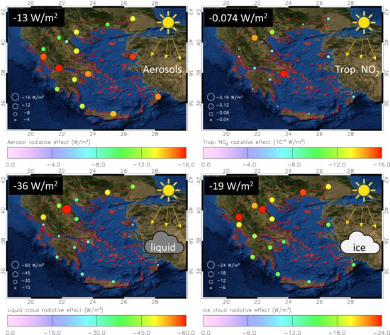
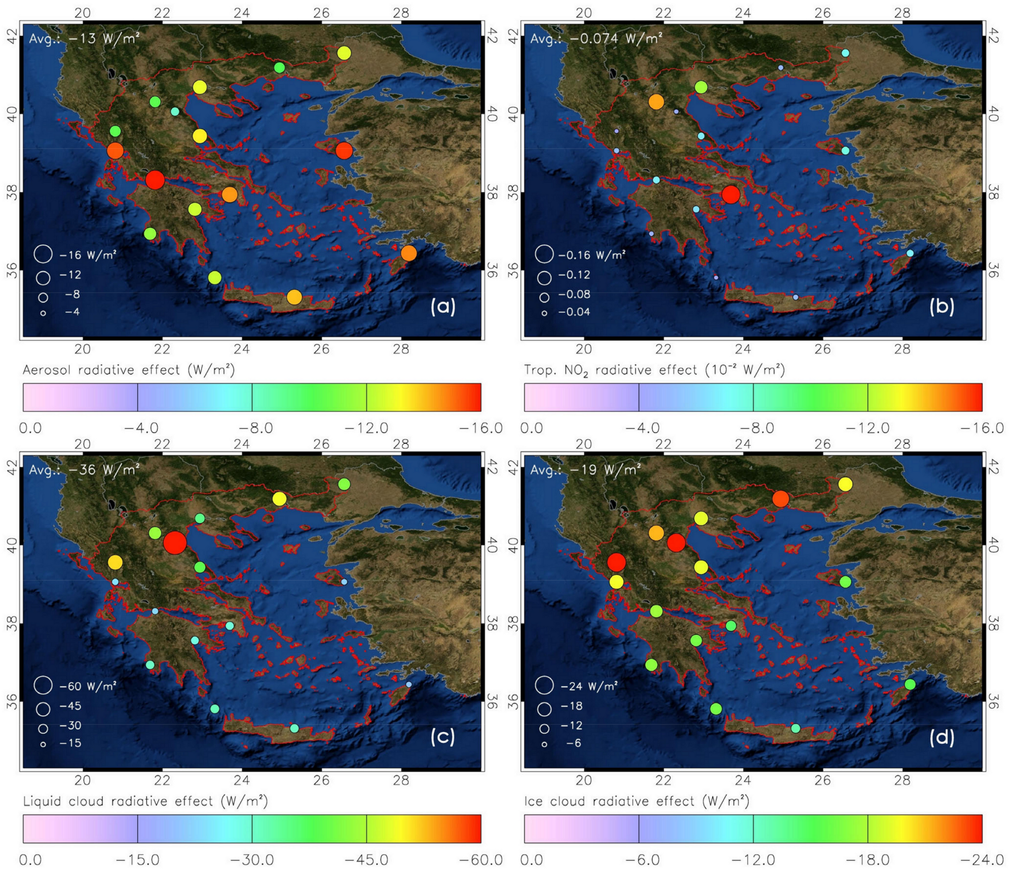
• The annual all-sky radiative effect of aerosols (RE_aer) and tropospheric NO₂ (RE_NO2) on SSR for the 16 locations in Greece is −13 W/m² and −0.074 W/m², respectively. Liquid clouds dominate, with an average RE_lc of −36 W/m², and ice clouds follow (RE_ic of −19 W/m²). RE_NO2 is smaller, by two orders of magnitude, compared to that of aerosols and clouds, and hence is negligible;
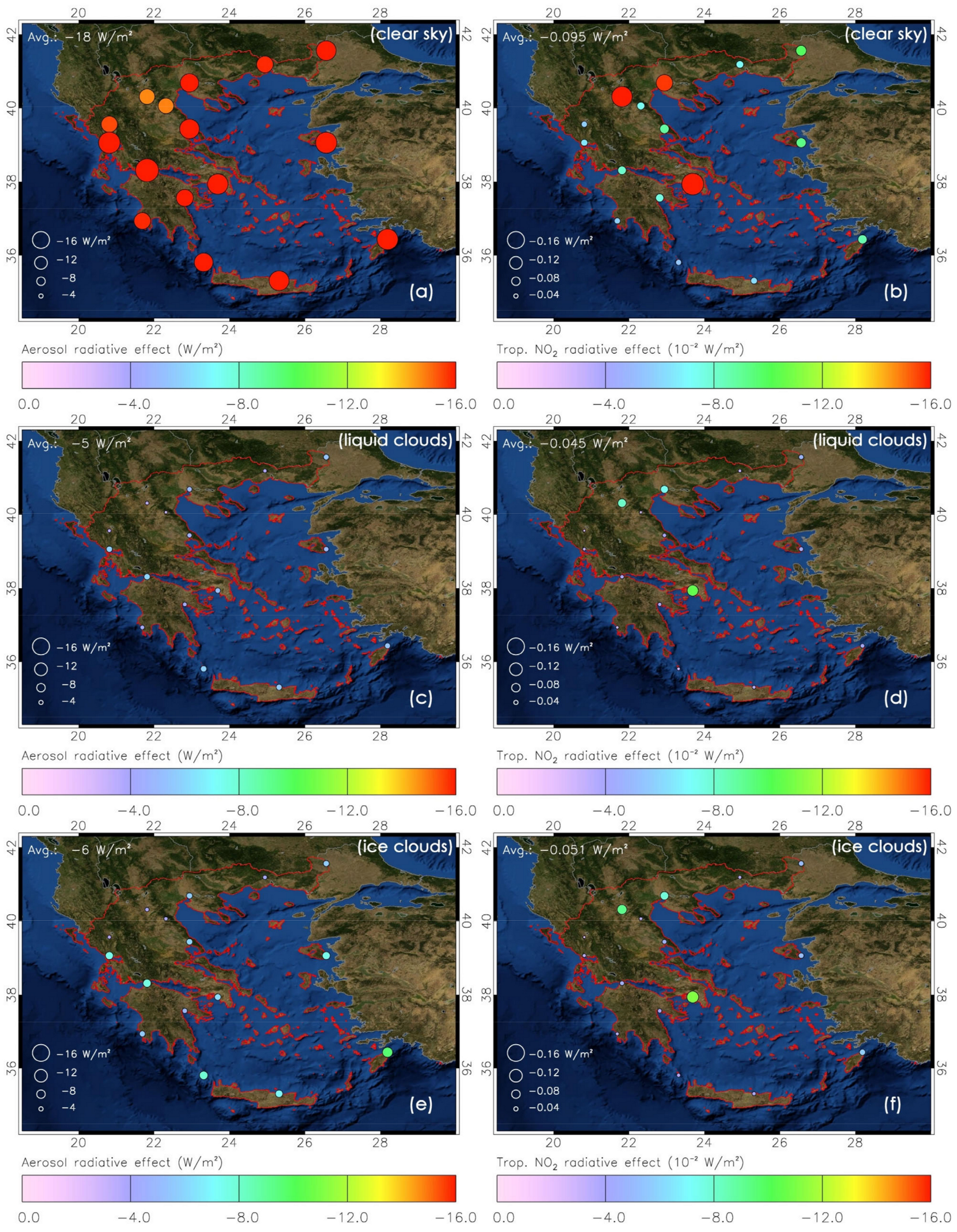
• On average, higher annual RE_aer values (by ~2 W/m²) appear over urban locations compared to rural locations. The annual RE_aer ranges from −18 W/m² (Patras) to −8 W/m² (Olympus). The annual RE_NO2 over urban locations (−0.113 W/m²) is double the ones over rural locations, with the highest values appearing over the three pollution hot spots in the area, namely, Athens (−0.166 W/m²), Kozani (−0.144 W/m²), and Thessaloniki (−0.118 W/m²). The annual RE_lc ranges spatially from −79 W/m² (Olympus) to −21 W/m² (Rhodes), while RE_ic ranges from −26 W/m² (Ioannina) to −13 W/m² (HCMR);
• The annual average RE_aer for all the locations under clear skies (−18 W/m²) is about 3–4 times larger than for liquid (−5 W/m²) and ice (−6 W/m²) cloud-covered skies; for individual locations, it can be up to 4–5 times larger (e.g., Olympus). For tropospheric NO₂, the average RE_NO2 under clear skies (−0.095 W/m²) is double that for liquid (−0.045 W/m²) and ice (−0.051 W/m²) cloud-covered skies;
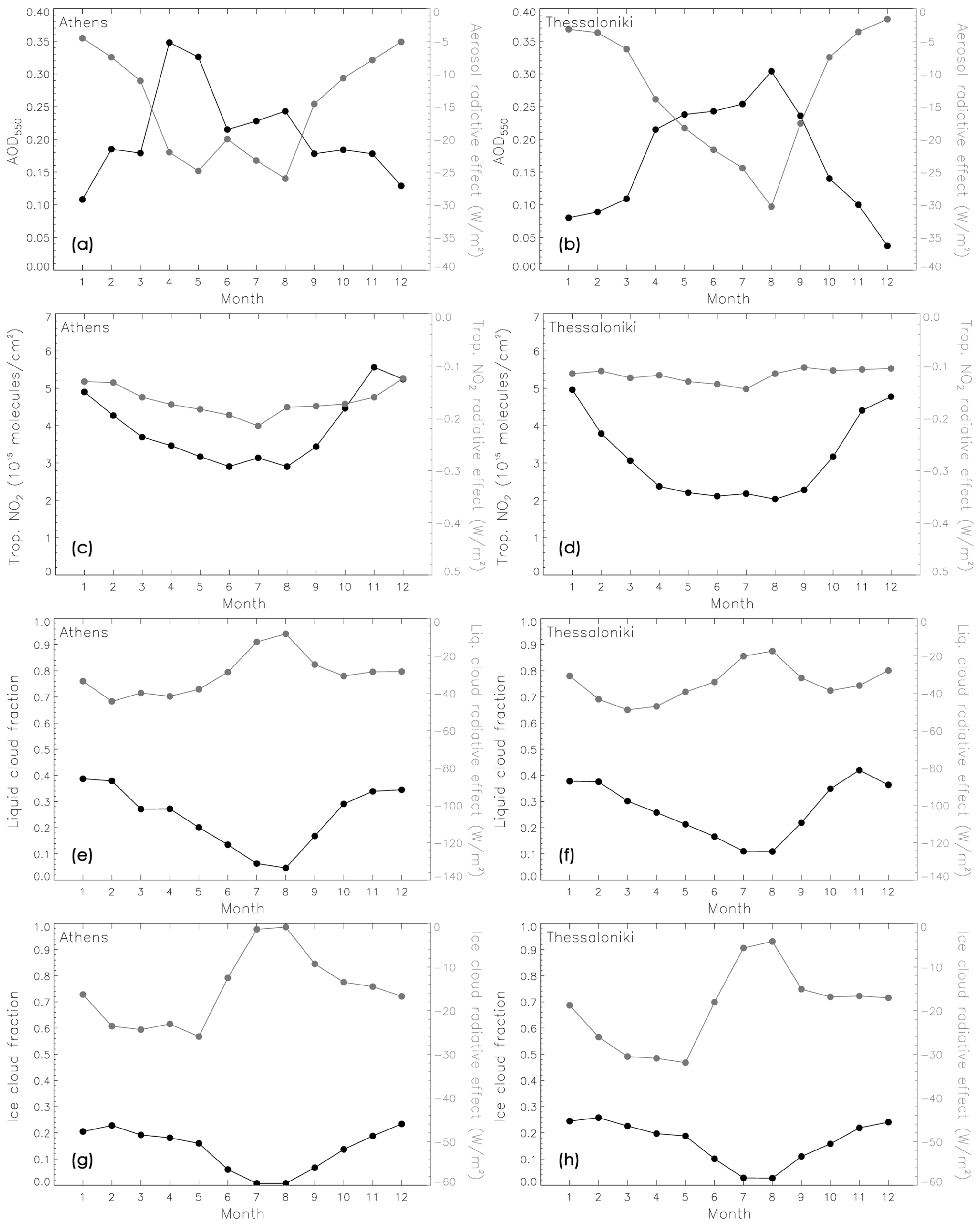
• RE_aer peaks in the spring and summer, with the maximum values (up to −30 W/m² for some locations) appearing in August over all the 16 locations. During the winter, especially in December and January, RE_aer generally drops below −5 W/m² and in some cases reaches values around −1 W/m². RE_NO2 peaks in July, with the highest values appearing over Athens (−0.215 W/m²), which is still very low to play a substantial role in the local radiative budget;
• The lowest RE_lc (−1 W/m²) appears in July over Rhodes, and the highest RE_lc (−123 W/m²) appears in May over Olympus. RE_ic is very low in the summer (July and August), ranging from −2 to 0 W/m² for 9 out of the 16 locations. The highest RE_ic value appears in May over Ioannina (−44 W/m²);
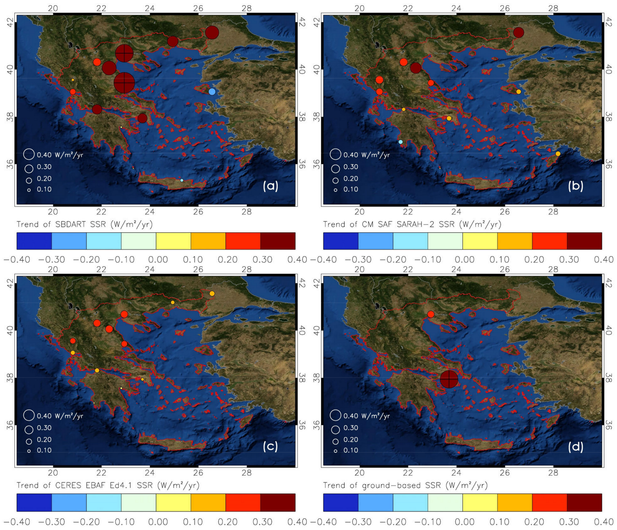
• Positive SSR trends (increase), ranging from 0.01 W/m²/year (Rhodes) to 0.52 W/m²/year (Olympus), appear over all the locations for the period 2005–2019, except for two, which are Mytilene (−0.27 W/m²/year or −0.14%/year) and HCMR (−0.12 W/m²/year or −0.06%/year). Over the two locations with the strongest trends, Volos (0.78 W/m²/year or 0.45%/year) and Thessaloniki (0.67 W/m²/year or 0.40%/year), the trends are statistically significant at the 95% confidence level. Our SSR trends, in general, agree with those of CM SAF (2005–2017) and CERES (2005–2019), indicating an increase in SSR over Athens and Thessaloniki, which is in agreement to the ground observations;
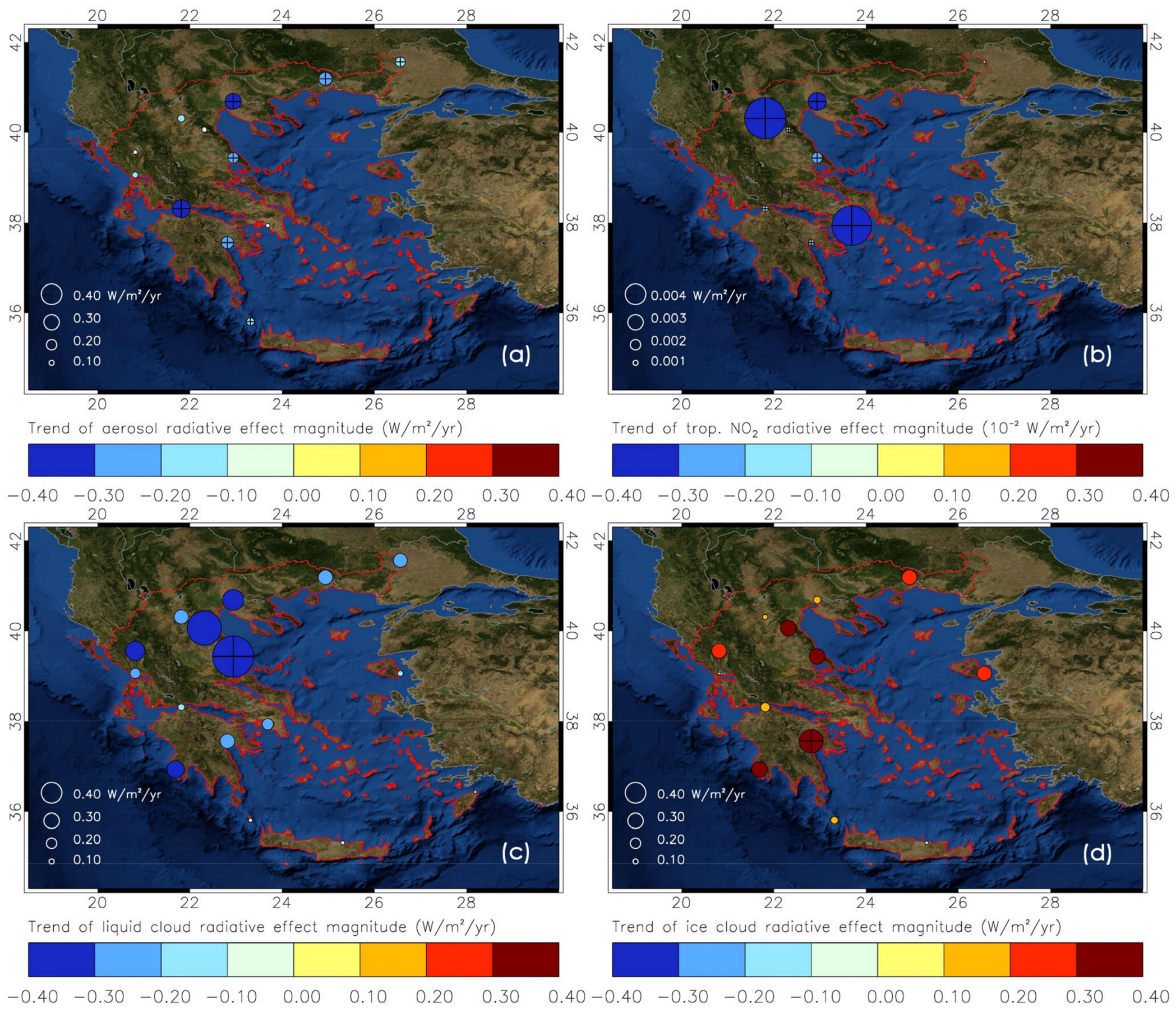
• The general decrease in AOD₅₅₀ (trends ranging from −0.005/year to zero depending on the location) and liquid cloud fraction (trends ranging from −0.006/year to −0.001/year) drives the positive SSR trends observed in the area for the period 2005–2019. The strongest RE_aer magnitude trends appear over the urban locations of Patras (−0.35 W/m²/year or −1.74%/year) and Thessaloniki (−0.31 W/m²/year or −2.05%/year), and the strongest RE_lc magnitude trend is found over the urban location of Volos (−0.80 W/m²/year or −1.78%/year). These three trend values are statistically significant at the 95% confidence level;
• The effect of tropospheric NO₂ on the SSR trends is negligible. Negative RE_NO2 magnitude trends (statistically significant for some locations only) are found over all the locations except for one (Antikythera). The negative RE_NO2 magnitude trends reflect the negative trends of tropospheric NO₂. The strongest tropospheric NO₂ trends (also statistically significant) are seen over the urban locations of Kozani (−0.21 × 10¹⁵ molecules/cm²/year or −3.95%/year), Athens (−0.19 × 10¹⁵ molecules/cm²/year or −3.57%/year), and Thessaloniki (−0.11 × 10¹⁵ molecules/cm²/year or −2.89%/year);
• Contrary to liquid clouds, the RE_ic magnitude exhibits positive trends over all the locations except for one (Rhodes). Argos exhibits the strongest trend (0.46 W/m²/year or 3.57%/year), being also the only location with a statistically significant trend. The positive RE_ic magnitude trends follow the positive ice cloud fraction trends (ranging from zero to 0.003/year depending on the location);
• The liquid and ice cloud optical thickness has increased for some stations, while for others it has decreased during 2005–2019, suppressing or boosting the changes in the radiative effect of clouds, which are induced by changes in the liquid and ice cloud fractions.

This study highlights the driving role of clouds and aerosols in the solar radiation levels reaching the Earth’s surface. Tropospheric NO₂ may exert a significant radiative effect on SSR on an annual basis, only over the most heavily polluted areas of the world (e.g., Eastern China). However, under episodic events (e.g., extended forest or agricultural fires), the instantaneous radiative effect of tropospheric NO₂ might be considerable on a local or regional scale. This is something that merits further investigation.

References

1. Teuling, A.J.; Hirschi, M.; Ohmura, A.; Wild, M.; Reichstein, M.; Ciais, P.; Buchmann, N.; Ammann, C.; Montagnani, L.; Richardson, A.D.; et al. A Regional Perspective on Trends in Continental Evaporation: EVAPORATION TRENDS. Geophys. Res. Lett. 2009, 36. [Google Scholar] [CrossRef] [Green Version]
2. Ramanathan, V. Aerosols, Climate, and the Hydrological Cycle. Science 2001, 294, 2119–2124. [Google Scholar] [CrossRef] [PubMed] [Green Version]
3. Wild, M.; Liepert, B. The Earth Radiation Balance as Driver of the Global Hydrological Cycle. Environ. Res. Lett. 2010, 5, 025203. [Google Scholar] [CrossRef]
4. Gu, L.; Baldocchi, D.; Verma, S.B.; Black, T.A.; Vesala, T.; Falge, E.M.; Dowty, P.R. Advantages of Diffuse Radiation for Terrestrial Ecosystem Productivity: ADVANTAGES OF DIFFUSE RADIATION. J. Geophys. Res. Atmos. 2002, 107, ACL 2-1-ACL 2-23. [Google Scholar] [CrossRef] [Green Version]
5. Mercado, L.M.; Bellouin, N.; Sitch, S.; Boucher, O.; Huntingford, C.; Wild, M.; Cox, P.M. Impact of Changes in Diffuse Radiation on the Global Land Carbon Sink. Nature 2009, 458, 1014–1017. [Google Scholar] [CrossRef] [Green Version]
6. Wild, M.; Folini, D.; Schär, C.; Loeb, N.; Dutton, E.G.; König-Langlo, G. The Global Energy Balance from a Surface Perspective. Clim. Dyn. 2013, 40, 3107–3134. [Google Scholar] [CrossRef] [Green Version]
7. Wild, M. Decadal Changes in Radiative Fluxes at Land and Ocean Surfaces and Their Relevance for Global Warming. Wiley Interdiscip. Rev. Clim. Change. 2016, 7, 91–107. [Google Scholar] [CrossRef]
8. Katragkou, E.; García-Díez, M.; Vautard, R.; Sobolowski, S.; Zanis, P.; Alexandri, G.; Cardoso, R.M.; Colette, A.; Fernandez, J.; Gobiet, A.; et al. Regional Climate Hindcast Simulations within EURO-CORDEX: Evaluation of a WRF Multi-Physics Ensemble. Geosci. Model Dev. 2015, 8, 603–618. [Google Scholar] [CrossRef] [Green Version]
9. Hammer, A.; Heinemann, D.; Hoyer, C.; Kuhlemann, R.; Lorenz, E.; Müller, R.; Beyer, H.G. Solar Energy Assessment Using Remote Sensing Technologies. Remote Sens. Environ. 2003, 86, 423–432. [Google Scholar] [CrossRef]
10. Wild, M.; Ohmura, A.; Schär, C.; Müller, G.; Folini, D.; Schwarz, M.; Hakuba, M.Z.; Sanchez-Lorenzo, A. The Global Energy Balance Archive (GEBA) Version 2017: A Database for Worldwide Measured Surface Energy Fluxes. Earth Syst. Sci. Data 2017, 9, 601–613. [Google Scholar] [CrossRef] [Green Version]
11. Driemel, A.; Augustine, J.; Behrens, K.; Colle, S.; Cox, C.; Cuevas-Agulló, E.; Denn, F.M.; Duprat, T.; Fukuda, M.; Grobe, H.; et al. Baseline Surface Radiation Network (BSRN): Structure and Data Description (1992–2017). Earth Syst. Sci. Data 2018, 10, 1491–1501. [Google Scholar] [CrossRef] [Green Version]
12. Pinker, R.T. Do Satellites Detect Trends in Surface Solar Radiation? Science 2005, 308, 850–854. [Google Scholar] [CrossRef] [Green Version]
13. Rossow, W.B.; Zhang, Y.-C. Calculation of Surface and Top of Atmosphere Radiative Fluxes from Physical Quantities Based on ISCCP Data Sets: 2. Validation and First Results. J. Geophys. Res. Atmos. 1995, 100, 1167–1197. [Google Scholar] [CrossRef]
14. Zhang, Y.; Rossow, W.B.; Lacis, A.; Oinas, V.; Mishchenko, M.I. Calculation of Radiative Fluxes from the Surface to Top of Atmosphere Based on ISCCP and Other Global Data Sets: Refinements of the Radiative Transfer Model and the Input Data. J. Geophys. Res. 2004, 109, D19105. [Google Scholar] [CrossRef] [Green Version]
15. Hatzianastassiou, N.; Matsoukas, C.; Fotiadi, A.; Pavlakis, K.G.; Drakakis, E.; Hatzidimitriou, D.; Vardavas, I. Global Distribution of Earth’s Surface Shortwave Radiation Budget. Atmos. Chem. Phys. 2005, 5, 2847–2867. [Google Scholar] [CrossRef] [Green Version]
16. Kim, D.; Ramanathan, V. Solar Radiation Budget and Radiative Forcing Due to Aerosols and Clouds. J. Geophys. Res. 2008, 113, D02203. [Google Scholar] [CrossRef] [Green Version]
17. Wang, H.; Pinker, R.T. Shortwave Radiative Fluxes from MODIS: Model Development and Implementation. J. Geophys. Res. 2009, 114, D20201. [Google Scholar] [CrossRef]
18. Müller, R.; Pfeifroth, U.; Träger-Chatterjee, C.; Trentmann, J.; Cremer, R. Digging the METEOSAT Treasure—3 Decades of Solar Surface Radiation. Remote Sens. 2015, 7, 8067–8101. [Google Scholar] [CrossRef] [Green Version]
19. Wang, Y.; Lyu, R.; Xie, X.; Meng, Z.; Huang, M.; Wu, J.; Mu, H.; Yu, Q.-R.; He, Q.; Cheng, T. Retrieval of Gridded Aerosol Direct Radiative Forcing Based on Multiplatform Datasets. Atmos. Meas. Tech. 2020, 13, 575–592. [Google Scholar] [CrossRef]
20. Giorgi, F. Climate Change Hot-Spots. Geophys. Res. Lett. 2006, 33, L08707. [Google Scholar] [CrossRef]
21. Papadimas, C.D.; Hatzianastassiou, N.; Matsoukas, C.; Kanakidou, M.; Mihalopoulos, N.; Vardavas, I. The Direct Effect of Aerosols on Solar Radiation over the Broader Mediterranean Basin. Atmos. Chem. Phys. 2012, 12, 7165–7185. [Google Scholar] [CrossRef] [Green Version]
22. Pyrina, M.; Hatzianastassiou, N.; Matsoukas, C.; Fotiadi, A.; Papadimas, C.D.; Pavlakis, K.G.; Vardavas, I. Cloud Effects on the Solar and Thermal Radiation Budgets of the Mediterranean Basin. Atmos. Res. 2015, 152, 14–28. [Google Scholar] [CrossRef]
23. Mateos, D.; Sanchez-Lorenzo, A.; Antón, M.; Cachorro, V.E.; Calbó, J.; Costa, M.J.; Torres, B.; Wild, M. Quantifying the Respective Roles of Aerosols and Clouds in the Strong Brightening since the Early 2000s over the Iberian Peninsula: RECENT BRIGHTENING BY CLOUDS AND AEROSOL. J. Geophys. Res. Atmos. 2014, 119, 10382–10393. [Google Scholar] [CrossRef] [Green Version]
24. Obregón, M.Á.; Serrano, A.; Costa, M.J.; Silva, A.M. Global Spatial and Temporal Variation of the Combined Effect of Aerosol and Water Vapour on Solar Radiation. Remote Sens. 2021, 13, 708. [Google Scholar] [CrossRef]
25. Hatzianastassiou, N.; Gkikas, A.; Mihalopoulos, N.; Torres, O.; Katsoulis, B.D. Natural versus Anthropogenic Aerosols in the Eastern Mediterranean Basin Derived from Multiyear TOMS and MODIS Satellite Data. J. Geophys. Res. 2009, 114, D24202. [Google Scholar] [CrossRef]
26. Georgoulias, A.K.; Alexandri, G.; Kourtidis, K.A.; Lelieveld, J.; Zanis, P.; Pöschl, U.; Levy, R.; Amiridis, V.; Marinou, E.; Tsikerdekis, A. Spatiotemporal Variability and Contribution of Different Aerosol Types to the Aerosol Optical Depth over the Eastern Mediterranean. Atmos. Chem. Phys. 2016, 16, 13853–13884. [Google Scholar] [CrossRef] [PubMed] [Green Version]
27. Alexandri, G.; Georgoulias, A.K.; Meleti, C.; Balis, D.; Kourtidis, K.A.; Sanchez-Lorenzo, A.; Trentmann, J.; Zanis, P. A High Resolution Satellite View of Surface Solar Radiation over the Climatically Sensitive Region of Eastern Mediterranean. Atmos. Res. 2017, 188, 107–121. [Google Scholar] [CrossRef]
28. Antón, M.; Mateos, D. Shortwave Radiative Forcing Due to Long-Term Changes of Total Ozone Column over the Iberian Peninsula. Atmos. Environ. 2013, 81, 532–537. [Google Scholar] [CrossRef]
29. Solomon, S.; Portmann, R.W.; Sanders, R.W.; Daniel, J.S.; Madsen, W.; Bartram, B.; Dutton, E.G. On the Role of Nitrogen Dioxide in the Absorption of Solar Radiation. J. Geophys. Res. Atmos. 1999, 104, 12047–12058. [Google Scholar] [CrossRef]
30. Vasilkov, A.P.; Joiner, J.; Oreopoulos, L.; Gleason, J.F.; Veefkind, P.; Bucsela, E.; Celarier, E.A.; Spurr, R.J.D.; Platnick, S. Impact of Tropospheric Nitrogen Dioxide on the Regional Radiation Budget. Atmos. Chem. Phys. 2009, 9, 6389–6400. [Google Scholar] [CrossRef] [Green Version]
31. Lohmann, U.; Feichter, J. Global Indirect Aerosol Effects: A Review. Atmos. Chem. Phys. 2005, 5, 715–737. [Google Scholar] [CrossRef] [Green Version]
32. Georgoulias, A.K.; van der A, R.J.; Stammes, P.; Boersma, K.F.; Eskes, H.J. Trends and Trend Reversal Detection in 2 Decades of Tropospheric NO2 Satellite Observations. Atmos. Chem. Phys. 2019, 19, 6269–6294. [Google Scholar] [CrossRef] [Green Version]
33. Salomonson, V.V.; Barnes, W.L.; Maymon, P.W.; Montgomery, H.E.; Ostrow, H. MODIS: Advanced Facility Instrument for Studies of the Earth as a System. IEEE Trans. Geosci. Remote Sens. 1989, 27, 145–153. [Google Scholar] [CrossRef]
34. Kaufman, Y.J.; Tanré, D.; Remer, L.A.; Vermote, E.F.; Chu, A.; Holben, B.N. Operational Remote Sensing of Tropospheric Aerosol over Land from EOS Moderate Resolution Imaging Spectroradiometer. J. Geophys. Res. Atmos. 1997, 102, 17051–17067. [Google Scholar] [CrossRef]
35. Remer, L.A.; Kaufman, Y.J.; Tanré, D.; Mattoo, S.; Chu, D.A.; Martins, J.V.; Li, R.-R.; Ichoku, C.; Levy, R.C.; Kleidman, R.G.; et al. The MODIS Aerosol Algorithm, Products, and Validation. J. Atmos. Sci. 2005, 62, 947–973. [Google Scholar] [CrossRef] [Green Version]
36. Levy, R.C.; Remer, L.A.; Kleidman, R.G.; Mattoo, S.; Ichoku, C.; Kahn, R.; Eck, T.F. Global Evaluation of the Collection 5 MODIS Dark-Target Aerosol Products over Land. Atmos. Chem. Phys. 2010, 10, 10399–10420. [Google Scholar] [CrossRef] [Green Version]
37. Levy, R.C.; Mattoo, S.; Munchak, L.A.; Remer, L.A.; Sayer, A.M.; Patadia, F.; Hsu, N.C. The Collection 6 MODIS Aerosol Products over Land and Ocean. Atmos. Meas. Tech. 2013, 6, 2989–3034. [Google Scholar] [CrossRef] [Green Version]
38. Tanré, D.; Kaufman, Y.J.; Herman, M.; Mattoo, S. Remote Sensing of Aerosol Properties over Oceans Using the MODIS/EOS Spectral Radiances. J. Geophys. Res. Atmos. 1997, 102, 16971–16988. [Google Scholar] [CrossRef]
39. Sayer, A.M.; Hsu, N.C.; Bettenhausen, C.; Jeong, M.-J. Validation and Uncertainty Estimates for MODIS Collection 6 “Deep Blue” Aerosol Data: DEEP BLUE COLLECTION 6 VALIDATION. J. Geophys. Res. Atmos. 2013, 118, 7864–7872. [Google Scholar] [CrossRef] [Green Version]
40. Sayer, A.M.; Munchak, L.A.; Hsu, N.C.; Levy, R.C.; Bettenhausen, C.; Jeong, M.-J. MODIS Collection 6 Aerosol Products: Comparison between Aqua’s e-Deep Blue, Dark Target, and “Merged” Data Sets, and Usage Recommendations. J. Geophys. Res. Atmos. 2014, 119, 965–13,989. [Google Scholar] [CrossRef]
41. Sayer, A.M.; Hsu, N.C.; Bettenhausen, C.; Jeong, M.-J.; Meister, G. Effect of MODIS Terra Radiometric Calibration Improvements on Collection 6 Deep Blue Aerosol Products: Validation and Terra/Aqua Consistency. J. Geophys. Res. Atmos. 2015, 120. [Google Scholar] [CrossRef] [Green Version]
42. Hsu, N.C.; Jeong, M.-J.; Bettenhausen, C.; Sayer, A.M.; Hansell, R.; Seftor, C.S.; Huang, J.; Tsay, S.-C. Enhanced Deep Blue Aerosol Retrieval Algorithm: The Second Generation: ENHANCED DEEP BLUE AEROSOL RETRIEVAL. J. Geophys. Res. Atmos. 2013, 118, 9296–9315. [Google Scholar] [CrossRef]
43. Hsu, N.C.; Lee, J.; Sayer, A.M.; Kim, W.; Bettenhausen, C.; Tsay, S.-C. VIIRS Deep Blue Aerosol Products Over Land: Extending the EOS Long-Term Aerosol Data Records. J. Geophys. Res. Atmos. 2019, 124, 4026–4053. [Google Scholar] [CrossRef]
44. Sayer, A.M.; Hsu, N.C.; Lee, J.; Kim, W.V.; Dutcher, S.T. Validation, Stability, and Consistency of MODIS Collection 6.1 and VIIRS Version 1 Deep Blue Aerosol Data Over Land. J. Geophys. Res. Atmos. 2019, 124, 4658–4688. [Google Scholar] [CrossRef]
45. Platnick, S.; Meyer, K.G.; King, M.D.; Wind, G.; Amarasinghe, N.; Marchant, B.; Arnold, G.T.; Zhang, Z.; Hubanks, P.A.; Holz, R.E.; et al. The MODIS Cloud Optical and Microphysical Products: Collection 6 Updates and Examples From Terra and Aqua. IEEE Trans. Geosci. Remote Sens. 2017, 55, 502–525. [Google Scholar] [CrossRef] [Green Version]
46. Ackerman, S.A.; Strabala, K.I.; Menzel, W.P.; Frey, R.A.; Moeller, C.C.; Gumley, L.E. Discriminating Clear Sky from Clouds with MODIS. J. Geophys. Res. Atmos. 1998, 103, 32141–32157. [Google Scholar] [CrossRef]
47. King, M.D.; Menzel, W.P.; Kaufman, Y.J.; Tanre, D.; Gao, B.-C.; Platnick, S.; Ackerman, S.A.; Remer, L.A.; Pincus, R.; Hubanks, P.A. Cloud and Aerosol Properties, Precipitable Water, and Profiles of Temperature and Water Vapor from MODIS. IEEE Trans. Geosci. Remote Sens. 2003, 41, 442–458. [Google Scholar] [CrossRef] [Green Version]
48. Platnick, S.; King, M.D.; Ackerman, S.A.; Menzel, W.P.; Baum, B.A.; Riedi, J.C.; Frey, R.A. The MODIS Cloud Products: Algorithms and Examples from Terra. IEEE Trans. Geosci. Remote Sens. 2003, 41, 459–473. [Google Scholar] [CrossRef] [Green Version]
49. Frey, R.A.; Ackerman, S.A.; Liu, Y.; Strabala, K.I.; Zhang, H.; Key, J.R.; Wang, X. Cloud Detection with MODIS. Part I: Improvements in the MODIS Cloud Mask for Collection 5. J. Atmospheric Ocean. Technol. 2008, 25, 1057–1072. [Google Scholar] [CrossRef]
50. Marchant, B.; Platnick, S.; Meyer, K.; Arnold, G.T.; Riedi, J. MODIS Collection 6 Shortwave-Derived Cloud Phase Classification Algorithm and Comparisons with CALIOP. Atmos. Meas. Tech. 2016, 9, 1587–1599. [Google Scholar] [CrossRef] [Green Version]
51. Nakajima, T.; King, M.D. Determination of the Optical Thickness and Effective Particle Radius of Clouds from Reflected Solar Radiation Measurements. Part I: Theory. J. Atmos. Sci. 1990, 47, 1878–1893. [Google Scholar] [CrossRef] [Green Version]
52. Menzel, W.P.; Frey, R.A.; Zhang, H.; Wylie, D.P.; Moeller, C.C.; Holz, R.E.; Maddux, B.; Baum, B.A.; Strabala, K.I.; Gumley, L.E. MODIS Global Cloud-Top Pressure and Amount Estimation: Algorithm Description and Results. J. Appl. Meteorol. Climatol. 2008, 47, 1175–1198. [Google Scholar] [CrossRef] [Green Version]
53. Baum, B.A.; Menzel, W.P.; Frey, R.A.; Tobin, D.C.; Holz, R.E.; Ackerman, S.A.; Heidinger, A.K.; Yang, P. MODIS Cloud-Top Property Refinements for Collection 6. J. Appl. Meteorol. Climatol. 2012, 51, 1145–1163. [Google Scholar] [CrossRef]
54. Kinne, S. The MACv2 Aerosol Climatology. Tellus B Chem. Phys. Meteorol. 2019, 71, 1–21. [Google Scholar] [CrossRef] [Green Version]
55. Winker, D.M.; Vaughan, M.A.; Omar, A.; Hu, Y.; Powell, K.A.; Liu, Z.; Hunt, W.H.; Young, S.A. Overview of the CALIPSO Mission and CALIOP Data Processing Algorithms. J. Atmos. Ocean. Technol. 2009, 26, 2310–2323. [Google Scholar] [CrossRef]
56. Hunt, W.H.; Winker, D.M.; Vaughan, M.A.; Powell, K.A.; Lucker, P.L.; Weimer, C. CALIPSO Lidar Description and Performance Assessment. J. Atmos. Ocean. Technol. 2009, 26, 1214–1228. [Google Scholar] [CrossRef]
57. Tackett, J.L.; Winker, D.M.; Getzewich, B.J.; Vaughan, M.A.; Young, S.A.; Kar, J. CALIPSO Lidar Level 3 Aerosol Profile Product: Version 3 Algorithm Design. Atmos. Meas. Tech. 2018, 11, 4129–4152. [Google Scholar] [CrossRef] [Green Version]
58. Young, S.A.; Vaughan, M.A.; Garnier, A.; Tackett, J.L.; Lambeth, J.D.; Powell, K.A. Extinction and Optical Depth Retrievals for CALIPSO’s Version 4 Data Release. Atmos. Meas. Tech. 2018, 11, 5701–5727. [Google Scholar] [CrossRef] [Green Version]
59. Boersma, K.F.; Eskes, H.J.; Richter, A.; De Smedt, I.; Lorente, A.; Beirle, S.; van Geffen, J.H.G.M.; Zara, M.; Peters, E.; Van Roozendael, M.; et al. Improving Algorithms and Uncertainty Estimates for Satellite NO2 Retrievals: Results from the Quality Assurance for the Essential Climate Variables (QA4ECV) Project. Atmos. Meas. Tech. 2018, 11, 6651–6678. [Google Scholar] [CrossRef] [Green Version]
60. Levelt, P.F.; Joiner, J.; Tamminen, J.; Veefkind, J.P.; Bhartia, P.K.; Stein Zweers, D.C.; Duncan, B.N.; Streets, D.G.; Eskes, H.; van der A, R.; et al. The Ozone Monitoring Instrument: Overview of 14 Years in Space. Atmos. Chem. Phys. 2018, 18, 5699–5745. [Google Scholar] [CrossRef] [Green Version]
61. Lorente, A.; Folkert Boersma, K.; Yu, H.; Dörner, S.; Hilboll, A.; Richter, A.; Liu, M.; Lamsal, L.N.; Barkley, M.; De Smedt, I.; et al. Structural Uncertainty in Air Mass Factor Calculation for NO2 and HCHO Satellite Retrievals. Atmos. Meas. Tech. 2017, 10, 759–782. [Google Scholar] [CrossRef] [Green Version]
62. Zara, M.; Boersma, K.F.; De Smedt, I.; Richter, A.; Peters, E.; van Geffen, J.H.G.M.; Beirle, S.; Wagner, T.; Van Roozendael, M.; Marchenko, S.; et al. Improved Slant Column Density Retrieval of Nitrogen Dioxide and Formaldehyde for OMI and GOME-2A from QA4ECV: Intercomparison, Uncertainty Characterisation, and Trends. Atmos. Meas. Tech. 2018, 11, 4033–4058. [Google Scholar] [CrossRef] [Green Version]
63. Pinardi, G.; Van Roozendael, M.; Hendrick, F.; Theys, N.; Abuhassan, N.; Bais, A.; Boersma, F.; Cede, A.; Chong, J.; Donner, S.; et al. Validation of Tropospheric NO2 Column Measurements of GOME-2A and OMI Using MAX-DOAS and Direct Sun Network Observations. Atmos. Meas. Tech. 2020, 13, 6141–6174. [Google Scholar] [CrossRef]
64. Compernolle, S.; Verhoelst, T.; Pinardi, G.; Granville, J.; Hubert, D.; Keppens, A.; Niemeijer, S.; Rino, B.; Bais, A.; Beirle, S.; et al. Validation of Aura-OMI QA4ECV NO2 Climate Data Records with Ground-Based DOAS Networks: The Role of Measurement and Comparison Uncertainties. Atmos. Chem. Phys. 2020, 20, 8017–8045. [Google Scholar] [CrossRef]
65. Pfeifroth, U.; Kothe, S.; Trentmann, J.; Hollmann, R.; Fuchs, P.; Kaiser, J.; Werscheck, M. Surface Radiation Data Set—Heliosat (SARAH)—Edition 2.1; Satellite Application Facility on Climate Monitoring: Offenbach, Germany, 2019. [Google Scholar] [CrossRef]
66. Pfeifroth, U.; Sanchez-Lorenzo, A.; Manara, V.; Trentmann, J.; Hollmann, R. Trends and Variability of Surface Solar Radiation in Europe Based On Surface- and Satellite-Based Data Records. J. Geophys. Res. Atmos. 2018, 123, 1735–1754. [Google Scholar] [CrossRef]
67. Loeb, N.G.; Doelling, D.R.; Wang, H.; Su, W.; Nguyen, C.; Corbett, J.G.; Liang, L.; Mitrescu, C.; Rose, F.G.; Kato, S. Clouds and the Earth’s Radiant Energy System (CERES) Energy Balanced and Filled (EBAF) Top-of-Atmosphere (TOA) Edition-4.0 Data Product. J. Clim. 2018, 31, 895–918. [Google Scholar] [CrossRef]
68. Kato, S.; Rose, F.G.; Rutan, D.A.; Thorsen, T.J.; Loeb, N.G.; Doelling, D.R.; Huang, X.; Smith, W.L.; Su, W.; Ham, S.-H. Surface Irradiances of Edition 4.0 Clouds and the Earth’s Radiant Energy System (CERES) Energy Balanced and Filled (EBAF) Data Product. J. Clim. 2018, 31, 4501–4527. [Google Scholar] [CrossRef]
69. Wielicki, B.A.; Barkstrom, B.R.; Harrison, E.F.; Lee III, R.B.; Smith, G.L.; Cooper, J.E. Clouds and the Earth’s Radiant Energy System (CERES): An Earth Observing System Experiment. Bull. Am. Meteorol. Soc. 1996, 77, 853–868. [Google Scholar] [CrossRef] [Green Version]
70. Loeb, N.G.; Priestley, K.J.; Kratz, D.P.; Geier, E.B.; Green, R.N.; Wielicki, B.A.; Hinton, P.O.; Nolan, S.K. Determination of Unfiltered Radiances from the Clouds and the Earth’s Radiant Energy System Instrument. J. Appl. Meteorol. Climatol. 2001, 40, 822–835 14. [Google Scholar] [CrossRef]
71. Su, W.; Corbett, J.; Eitzen, Z.; Liang, L. Next-Generation Angular Distribution Models for Top-of-Atmosphere Radiative Flux Calculation from CERES Instruments: Methodology. Atmos. Meas. Tech. 2015, 8, 611–632. [Google Scholar] [CrossRef] [Green Version]
72. Bais, A.F.; Drosoglou, T.; Meleti, C.; Tourpali, K.; Kouremeti, N. Changes in Surface Shortwave Solar Irradiance from 1993 to 2011 at Thessaloniki (Greece): SHORTWAVE DOWNWARD SOLAR IRRADIANCE TREND. Int. J. Climatol. 2013, 33, 2871–2876. [Google Scholar] [CrossRef] [Green Version]
73. Kazadzis, S.; Founda, D.; Psiloglou, B.E.; Kambezidis, H.; Mihalopoulos, N.; Sanchez-Lorenzo, A.; Meleti, C.; Raptis, P.I.; Pierros, F.; Nabat, P. Long-Term Series and Trends in Surface Solar Radiation in Athens, Greece. Atmos. Chem. Phys. 2018, 18, 2395–2411. [Google Scholar] [CrossRef] [Green Version]
74. Bhartia, P.K. OMI/Aura TOMS-Like Ozone, Aerosol Index, Cloud Radiance Fraction Daily L3 Global 1.0 × 1.0 Deg; Goddard Earth Sciences Data and Information Services Center: Greenbelt, MD, USA, 2012. [CrossRef]
75. Karlsson, K.-G.; Anttila, K.; Trentmann, J.; Stengel, M.; Solodovnik, I.; Meirink, J.F.; Devasthale, A.; Kothe, S.; Jääskeläinen, E.; Sedlar, J.; et al. CLARA-A2.1: CM SAF CLoud, Albedo and Surface RAdiation Dataset from AVHRR Data—Edition 2.1; Satellite Application Facility on Climate Monitoring: Offenbach, Germany, 2020. [Google Scholar] [CrossRef]
76. Finkensieper, S.; Meirink, J.F.; van Zadelhoff, G.-J.; Hanschmann, T.; Benas, N.; Stengel, M.; Fuchs, P.; Hollmann, R.; Kaiser, J.; Werscheck, M. CLAAS-2.1: CM SAF CLoud Property DAtAset Using SEVIRI—Edition 2.1; Satellite Application Facility on Climate Monitoring: Offenbach, Germany, 2020. [Google Scholar] [CrossRef]
77. Danielson, J.J.; Gesch, D.B. Global Multi-Resolution Terrain Elevation Data 2010 (GMTED2010). US Geol. Surv. 2011, 23. [Google Scholar] [CrossRef]
78. Center For International Earth Science Information Network-CIESIN-Columbia University Gridded Population of the World, Version 4 (GPWv4): Population Count, Revision 11; CIESIN: New York, NY, USA, 2018. [CrossRef]
79. Ricchiazzi, P.; Yang, S.; Gautier, C.; Sowle, D. SBDART: A Research and Teaching Software Tool for Plane-Parallel Radiative Transfer in the Earth’s Atmosphere. Bull. Am. Meteorol. Soc. 1998, 79, 2101–2114. [Google Scholar] [CrossRef] [Green Version]
80. Hatzianastassiou, N.; Vardavas, I. Shortwave Radiation Budget of the Northern Hemisphere Using International Satellite Cloud Climatology Project and NCEP/NCAR Climatological Data. J. Geophys. Res. Atmos. 1999, 104, 24401–24421. [Google Scholar] [CrossRef] [Green Version]
81. McClatchey, R.A.; Fenn, R.W.; Shelby, J.E.A.; Voltz, F.E.; Garing, J.S. Optical Properties of the Atmosphere; AFCRL-71-0279; Air Force Geophysics Laboratory: Bedford, MA, USA, 1972. [Google Scholar]
82. Korolev, A.; Isaac, G.A. Relative Humidity in Liquid, Mixed-Phase, and Ice Clouds. J. Atmos. Sci. 2006, 63, 2865–2880. [Google Scholar] [CrossRef] [Green Version]
83. Burrows, J.P.; Dehn, A.; Deters, B.; Himmelmann, S.; Richter, A.; Voigt, S.; Orphal, J. Atmospheric remote-sensing reference data from gome: Part 1. temperature-dependent absorption cross-sections of NO2 in the 231–794 Nm RANGE. J. Quant. Spectrosc. Radiat. Transf. 1998, 60, 1025–1031. [Google Scholar] [CrossRef]
84. Vardavas, I.M.; Koutoulaki, K. A Model for the Solar Radiation Budget of the Northern Hemisphere: Comparison with Earth Radiation Budget Experiment Data. J. Geophys. Res. 1995, 100, 7303–7314. [Google Scholar] [CrossRef]
85. Hatzianastassiou, N.; Katsoulis, B.; Vardavas, I. Global Distribution of Aerosol Direct Radiative Forcing in the Ultraviolet and Visible Arising under Clear Skies. Tellus B Chem. Phys. Meteorol. 2004, 56, 51–71. [Google Scholar] [CrossRef]
86. Benas, N.; Hatzianastassiou, N.; Matsoukas, C.; Fotiadi, A.; Mihalopoulos, N.; Vardavas, I. Aerosol Shortwave Direct Radiative Effect and Forcing Based on MODIS Level 2 Data in the Eastern Mediterranean (Crete). Atmos. Chem. Phys. 2011, 11, 12647–12662. [Google Scholar] [CrossRef] [Green Version]
87. Bais, A.F.; Kazantzidis, A.; Zerefos, C.S.; Melas, D.; Kosmidis, E.; Kazadzis, S.; Nikitidou, E.; Giannaros, T.M.; Zempila, M.-M.; Fragkos, K.; et al. Hellenic Network for Solar Energy. In Advances in Meteorology, Climatology and Atmospheric Physics; Helmis, C.G., Nastos, P.T., Eds.; Springer Atmospheric Sciences: Berlin/Heidelberg, Germany, 2013; pp. 391–396. ISBN 978-3-642-29171-5. [Google Scholar]
88. Kampouri, A.; Amiridis, V.; Solomos, S.; Gialitaki, A.; Marinou, E.; Spyrou, C.; Georgoulias, A.K.; Akritidis, D.; Papagiannopoulos, N.; Mona, L.; et al. Investigation of Volcanic Emissions in the Mediterranean: “The Etna–Antikythera Connection”. Atmosphere 2020, 12, 40. [Google Scholar] [CrossRef]
89. Weatherhead, E.C.; Reinsel, G.C.; Tiao, G.C.; Meng, X.-L.; Choi, D.; Cheang, W.-K.; Keller, T.; DeLuisi, J.; Wuebbles, D.J.; Kerr, J.B.; et al. Factors Affecting the Detection of Trends: Statistical Considerations and Applications to Environmental Data. J. Geophys. Res. Atmos. 1998, 103, 17149–17161. [Google Scholar] [CrossRef]
90. Georgoulias, A.K.; Alexandri, G.; Kourtidis, K.A.; Lelieveld, J.; Zanis, P.; Amiridis, V. Differences between the MODIS Collection 6 and 5.1 Aerosol Datasets over the Greater Mediterranean Region. Atmos. Environ. 2016, 147, 310–319. [Google Scholar] [CrossRef]
91. Pozzer, A.; de Meij, A.; Yoon, J.; Tost, H.; Georgoulias, A.K.; Astitha, M. AOD Trends during 2001–2010 from Observations and Model Simulations. Atmos. Chem. Phys. 2015, 15, 5521–5535. [Google Scholar] [CrossRef] [Green Version]
92. Zhang, X.; Liang, S.; Wild, M.; Jiang, B. Analysis of Surface Incident Shortwave Radiation from Four Satellite Products. Remote Sens. Environ. 2015, 165, 186–202. [Google Scholar] [CrossRef]
93. Wang, Y.; Trentmann, J.; Yuan, W.; Wild, M. Validation of CM SAF CLARA-A2 and SARAH-E Surface Solar Radiation Datasets over China. Remote Sens. 2018, 10, 1977. [Google Scholar] [CrossRef] [Green Version]
94. Pyrina, M.; Papadimas, C.D.; Fotiadi, A.; Matsoukas, C.; Hatzianastassiou, N.; Vardavas, I. Cloud Radiative Effects on Solar Radiation Over the Eastern Mediterranean Basin from 1984 to 2007. In Advances in Meteorology, Climatology and Atmospheric Physics; Helmis, C.G., Nastos, P.T., Eds.; Springer Atmospheric Sciences: Berlin/Heidelberg, Germany, 2013; pp. 693–699. ISBN 978-3-642-29171-5. [Google Scholar]
95. Alexandri, G.; Georgoulias, A.K.; Zanis, P.; Katragkou, E.; Tsikerdekis, A.; Kourtidis, K.; Meleti, C. On the Ability of RegCM4 Regional Climate Model to Simulate Surface Solar Radiation Patterns over Europe: An Assessment Using Satellite-Based Observations. Atmos. Chem. Phys. 2015, 15, 13195–13216. [Google Scholar] [CrossRef] [Green Version]
96. Kambezidis, H.D.; Kaskaoutis, D.G.; Kalliampakos, G.K.; Rashki, A.; Wild, M. The Solar Dimming/Brightening Effect over the Mediterranean Basin in the Period 1979–2012. J. Atmos. Sol.-Terr. Phys. 2016, 150–151, 31–46. [Google Scholar] [CrossRef]
97. Hatzianastassiou, N.; Ioannidis, E.; Korras-Carraca, M.-B.; Gavrouzou, M.; Papadimas, C.D.; Matsoukas, C.; Benas, N.; Fotiadi, A.; Wild, M.; Vardavas, I. Global Dimming and Brightening Features during the First Decade of the 21st Century. Atmosphere 2020, 11, 308. [Google Scholar] [CrossRef] [Green Version]
98. Cronin, T.W. On the Choice of Average Solar Zenith Angle. J. Atmospheric Sci. 2014, 71, 2994–3003. [Google Scholar] [CrossRef]
99. Kosmopoulos, P.G.; Kazadzis, S.; Taylor, M.; Athanasopoulou, E.; Speyer, O.; Raptis, P.I.; Marinou, E.; Proestakis, E.; Solomos, S.; Gerasopoulos, E.; et al. Dust Impact on Surface Solar Irradiance Assessed with Model Simulations, Satellite Observations and Ground-Based Measurements. Atmos. Meas. Tech. 2017, 10, 2435–2453. [Google Scholar] [CrossRef] [Green Version]
100. Tzoumanikas, P.; Nikitidou, E.; Bais, A.F.; Kazantzidis, A. The Effect of Clouds on Surface Solar Irradiance, Based on Data from an All-Sky Imaging System. Renew. Energy 2016, 95, 314–322. [Google Scholar] [CrossRef]
101. Schutgens, N.; Tsyro, S.; Gryspeerdt, E.; Goto, D.; Weigum, N.; Schulz, M.; Stier, P. On the Spatio-Temporal Representativeness of Observations. Atmos. Chem. Phys. 2017, 17, 9761–9780. [Google Scholar] [CrossRef] [Green Version]
Figure 1. Flowchart with the datasets, the methodology and the radiative transfer system used in this work. Dark grey is used for the core and light grey for the ancillary data.
Remotesensing 13 02587 g001
Figure 2. Maps with the (a) topography (in meters above sea level—m.a.s.l.), (b) annual average MODIS/Aqua AOD550, and (c) annual average OMI/AURA tropospheric NO2 VCD (in 1015 molecules/cm2) over the area of interest for the period 2005–2019. The grid cells with the 16 locations in Greece examined in this work are also indicated.
Remotesensing 13 02587 g002
Figure 3. Scatterplot of monthly mean SSR data produced in this work based on SBDART and (a) ground-based SSR observations from Thessaloniki, Athens, and HCMR; (c) CM SAF SARAH-2.1 SSR data from all the 16 locations that are studied here; and (d) CERES EBAF edition 4.1 SSR data from all the 16 locations that are studied here. The grey open circles represent the collocation points, the solid line is the regression line and the dashed line is the 1:1 line. The regression line (slope and offset with the corresponding ±1σ) and the correlation coefficient R, the MB, MAB, NMB, RMSE and the number of collocation points are also given on the plots. The (b,d,f) plots are the same as the (a,c,e) plots, respectively, but for deseasonalized timeseries.
Remotesensing 13 02587 g003
Figure 4. Annual average radiative effect of (a) aerosols, (b) tropospheric NO2, (c) liquid clouds and (d) ice clouds over 16 locations in Greece for the period 2005−2019. Mind that a different scale is used for the radiative effect of each parameter and that the radiative effect of tropospheric NO2 is smaller by two orders of magnitude.
Remotesensing 13 02587 g004
Figure 5. Maps with the annual average MODIS/Aqua (a) liquid cloud fraction, (b) ice cloud fraction, (c) liquid cloud optical thickness and (d) ice cloud optical thickness over the area of interest for the period 2005–2019.
Remotesensing 13 02587 g005
Figure 6. Annual average radiative effect of aerosols and tropospheric NO2 for (a,b) clear, (c,d) liquid and (e,f) ice cloud-covered skies over 16 locations in Greece for the period 2005–2019. Mind that a different scale is used for the two parameters and that the radiative effect of tropospheric NO2 is smaller by two orders of magnitude.
Remotesensing 13 02587 g006
Figure 7. Seasonal variability of AOD550, tropospheric NO2 VCD, liquid cloud fraction and ice cloud fraction (black color) with the corresponding aerosol, tropospheric NO2, liquid cloud and ice cloud radiative effect (grey color) for Athens (a,c,e,g) and Thessaloniki (b,d,f,h) during the period 2005–2019. Aerosol- and cloud-related parameters are from MODIS/Aqua and tropospheric NO2 from OMI/Aura.
Remotesensing 13 02587 g007
Figure 8. SSR trend for the period 2005–2019 over 16 locations in Greece based on (a) data produced here with SBDART, (b) CM SAF SARAH-2.1 SSR data and (c) CERES EBAF edition 4.1 SSR data. (d) SSR trend based on ground-based observations from the stations of Athens and Thessaloniki. Statistically significant trends at the 95% confidence level are indicated with a cross.
Remotesensing 13 02587 g008
Figure 9. Trend of the radiative effect of (a) aerosols, (b) tropospheric NO2, (c) liquid clouds and (d) ice clouds for the period 2005–2019 over 16 locations in Greece. Statistically significant trends at the 95% confidence level are indicated with a cross.
Remotesensing 13 02587 g009
Figure 10. Relative trend (to the first year) of (a) AOD550, (b) tropospheric NO2, (c) liquid cloud fraction and (d) ice cloud fraction, (e) liquid cloud optical thickness and (f) ice cloud optical thickness for the period 2005–2019 over 16 locations in Greece. Statistically significant trends at the 95% confidence level are indicated with a cross. Aerosol- and cloud-related parameters are from MODIS/Aqua and tropospheric NO2 from OMI/Aura.
Remotesensing 13 02587 g010