Abstract
Black soil areas are strongly affected by rill erosion due to the geomorphic characteristics of flood plains and heavy rainfall. To study the problem of rill erosion in black soil areas and achieve ecological restoration, based on the method of artificially simulated rainfall, the effects of rainfall intensity and slope on the characteristics of flow and sand production on the slope surface of black soil areas were studied, and the erosion pattern of the slope surface after rainfall was monitored by a 3D laser scanner to analyze the erosion of the soil on the slope surface. The slope erosion model was constructed on the basis of the cellular automata (CA) method, and the results of the model’s operation were compared with actual rainfall measurement results to deepen research on the slope erosion mechanism in black soil areas. By analyzing the slope erosion pattern after rainfall, it was found that the surface area and erosion volume of serious slope erosion areas increased with increases in slope gradient. Based on the physical model test results combined with the CA model to simulate flow and sand production on bare slopes under different rainfall intensities, comparison showed that the CA model can accurately simulate flow and sand production on a slope where the Ens coefficient of the flow production rate is between 0.70 and 0.97, thus theoretically verifying the reliability of the model, and on this basis, the erosion pattern of the slope after rainfall was predicted to explore the evolution and development law of erosion.
1. Introduction
As one of the three major black soil regions in the world, the northeast black soil region of China has scarce black soil resources but bears the main task of grain production [1]. The region has typical characteristics of a floodplain [2] that has been seriously affected by rill erosion under the action of rainfall over a long period, which has limited the economic and agricultural development of its black soil area. Therefore, the prevention and control of soil and water loss play a vital role in the restoration of this black soil area.
With the development of digital photogrammetry technology, digital elevation models (DEMs) generated by this technology have been widely used in scientific research on geomorphologic evolution. Welth et al. [3] used non-metric cameras and digital instruments to measure valleys and rivers and estimate rill erosion. Dymond et al. [4] used the traditional stereo mapping instrument to measure a watershed in New Zealand. The rill erosion of the whole watershed was calculated by the elevation change of the surface of the watershed. Gizaw et al. [5] used close-range photogrammetry technology to analyze the micro-geomorphology characteristics of a residential area in the field, and the results showed that the relative error of DSM data generated by this technology was about 2.8 mm. Kristen et al. [6] carried out photogrammetry on the topography of a canyon area using a consumer unmanned aerial vehicle (UAV) and compared the data obtained with the data obtained using three laser radars. Vinci et al. [7] used structure from motion (SFM) technology to measure slopes with smartphone cameras, and the results showed that the rill erosion estimated by SFM was comparable to the accuracy of 3D laser scanning. Currently, 3D laser scanning is widely used in engineering measurement, topography, and other fields. Huang, the director of the U. S. Soil Erosion Laboratory, has been measuring the micro-topography in runoff erosion areas with a self-made three-dimensional laser scanner since the late 1980s. David et al. [8] used three-dimensional laser scanning technology to calculate the deposition and erosion of rivers, but the results showed that submerged areas (<0.2 m depth) returned lower precision, with a range of −0.15 to +0.06 m. Eitel et al. [9] evaluated the feasibility of applying three-dimensional laser scanning technology to study the influence of surface roughness on runoff erosion of grassland river channels. Magnus et al. [10] combined airborne three-dimensional laser scanning with ground three-dimensional laser scanning to quantitatively evaluate land subsidence caused by debris flow activities in valley areas with an area of more than 100 hm2. However, to further quantitatively evaluate rill erosion, we used the cellular automata model to predict the degree of rill erosion.
The theoretical model of cellular automata is widely used. In terms of physical definition, cellular automata refer to a dynamic system defined on a cellular space consisting of discrete and finite-state cells, which evolves in the discrete time dimension according to certain local rules. The rill erosion model based on cellular automata is different from the traditional empirical model and mechanical model; it is permeated with the idea of self-organization, possesses powerful parallel computing capability, uses a local-to-whole evolutionary approach, has uncertain evolutionary characteristics, and can show greater superiority in the process of stochastic scenario simulation. Since the 1990s, CA has been widely applied worldwide in the field of rill erosion. Smith [11] simulated the process of terrain erosion with a simple cellular automata model. Murray and Paola [12] established a CA model for simulating the shape of a river from the perspective of water flow and sediment transport. Through theoretical and practical comparisons, they succeeded in simulating the main characteristics of the phenomenon. Pilotti and Menduni [13] used a two-dimensional lattice gas model to simulate the surface erosion process and the transport process of eroded materials. D’Ambrosio [14] and others developed the "SCAVATU" model based on CA to simulate the process of soil water erosion. Wei [15] presented a model (LANDSAP) that extends the Gilbert model to combine both surface and subsurface processes. M. Bursik et al. [16] combined CA with a smooth particle hydrodynamics model to simulate slope degradation caused by slope flow. The model analyzed the relationship between slope and geomorphologic evolution. Valette [17] used CA to simulate the surface soil degradation caused by rainfall and used soil aggregates as a research object to generalize soil particles by a three-phase system. The processes of splash erosion, infiltration, runoff, transport, and deposition were simulated. Rinaldi et al. [18] used the CA method to define the local rules among cells, such as rainfall, infiltration, and evaporation, and developed a watershed hydrological model to simulate surface water flow. Yuan et al. [19] constructed a small watershed erosion and sand production process model based on meta-cellular automata using a small watershed in the hilly gully area of the Loess Plateau as an example. Narteau et al. [20] established a 3D cellular automaton model to simulate random processes such as erosion, deposition, and sediment transport. At the same time, a lattice gas cellular automaton was used to simulate the shear stress of water flow to reflect the feedback between water flow and riverbed, showing the change of a river channel. Yuan et al. [21] introduced CA theory and methods into simulation of the slope water erosion process, established a CA model of the slope fine gully development process, and verified and evaluated the model simulation results using an artificially simulated rainfall experiment supported by 3D laser scanner. Wu et al. [22] used the cellular automata model to preliminarily realize the visual simulation of the rill development process, but the simulated effect of average rill depth, maximum rill depth, and average rill width of the longest rill was not good, and there were still many details to be improved and considered. Sun et al. [23] studied rill erosion on a 26.8% slope using a ground laser scanner and cellular automaton model under simulated rainfall conditions, and accurately simulated the runoff process, but the simulation of the sediment process was poor. The study of soil erosion at the slope scale mainly focuses on fine gully erosion caused by slope surface flow, and the influencing factors are mainly rainfall intensity, subgrade conditions, and slope gradient. In the CA model of soil erosion, the above-mentioned influencing factors as meta-cell variables, together with water depth, runoff, and erosion volume, affect the change of the meta-cell state that is realized by the transformation rule, which is the core of the CA model. The infiltration and sediment transport are simulated by Horton’s formula and Manning’s formula, etc. The parameters in the formula are determined by experimental rates. Determining the flow direction, water-sand exchange, and sediment erosion is the focus of the CA model. The flow direction of this model uses the D8 algorithm; the water can only flow into eight adjacent cells.
In this paper, using a three-dimensional laser scanning test and cellular automata soil erosion model, we studied the effects of different rainfall intensities and slope on the characteristics of bare slope sediment yield in a black soil area. By exploring the morphological characteristics of the slope after rainfall, the dynamic process of slope erosion in the black soil area was revealed, providing theoretical guidance for erosion prevention and control measures in the black soil area.
2. Experimental Procedure and Theoretical Foundation
2.1. Experimental Procedure
In this experiment, artificial rainfall simulation was used to analyze the process of sediment production and loss. The Norton rainfall system was selected for the experiment. Rainfall intensity was 20–120 mm/h and controlled by pressure and nozzle size, rainfall uniformity was greater than 90%, the effective rainfall area was 2 × 4 m, and rainfall height was 5.5 m. The X-Scan 3D scanning system used the handheld fast scanning mode and scanned the space object by fringe projection. The resolution and accuracy could reach 0.1 mm. Using the method of feature stitching and marker point positioning, the continuous scene within the single scanning range was scanned rapidly, and the object length could reach 0.15–4.00 m.
For the rainfall simulation slope surface, a mobile variable-slope steel trough was used. The black soil test steel trough was 1.5 m long, 0.4 m wide, and 0.25 m deep. The loess test steel trough was 2, 3, and 4 m long and 0.5 m wide, and the slope variation range was 0–25°.The bottom of the steel tank was perforated evenly so that the water in the soil could permeate freely.
To simulate the real situation of rainfall, a layered soil filling method was adopted. The test soil was taken from a slope on the outer side of the second Songhua River main stream embankment; the mechanical composition of the test soil is shown in Table 1. In order to eliminate boundary influence, the boundary soil was compacted as much as possible. In the black soil test, the rainfall intensity was selected as 30 mm/h, 50 mm/h, and 70 mm/h [24], and the duration of rainfall was set as 1 h [25]. The time of runoff was recorded. Samples were taken every 3 min from the beginning of runoff, and the sampling time was 10 s. In the loess test, the rainfall intensity was selected as 40 mm/h, 80 mm/h, and 120 mm/h, respectively, and the rainfall duration was set as 30 min. After the end of rainfall, runoff sediment samples and total runoff sediment samples from each stage were taken to the laboratory for static precipitation, and then the volume of supernatant flow was measured with a measuring cylinder. The obtained sediment samples were dried to a constant weight in an oven at 105 °C, and the dry sediment was weighed. Because the black soil is more cohesive and has less internal deformation, the reformation of material inside the slope was ignored.

Table 1.
Mechanical composition of the soil under test.
2.2. Description of the CA Model
2.2.1. Model Structure
The following CA model for rill erosion by water, Simulation by Cellular Automata, can be seen as a two-dimensional plane, partitioned into square cells of uniform size:
where:
L = {(x,y)|x,y ∈ N, 0 ≤ x ≤ 1x, 0 ≤ y ≤ 1y} is the set of points with integer co-ordinates in the finite region where the phenomenon evolves. N is the set of natural numbers, and lx and ly represent the limits of the region. In this paper, the cellular automata model adopts a constant boundary. Assuming that no water and sand flow into the boundary of the upper cell, the water and sediment flow out of the boundary of the lower cell is regarded as the flow rate and sediment yield of the whole slope surface, and the flow direction on both sides of the boundary cell is determined as the direction toward the boundary.
Sz is the set of states of the cellular, described as follows:
Sg represents global variables, mainly including cell size, rainfall intensity, time step length, average slope, etc. Sl represents local variables, mainly including water depth, elevation, sand amount, etc. N represents the neighbor of the cell, and the mole neighbor cell is adopted.
N = {(0,−1),(0,1),(1,−1),(1,0),(1,1),(−1,−1),(−1,0),(−1,−1)}. In the CA model, only water and sand interactions occur between the cell and its neighboring cell. The rules of each cell are consistent with those of its neighbors.
In addition, this model adopts the boundary cell at the top of the constant value boundary in which no water and sand flow into the cell. The water flow and sediment flow out of the boundary cell at the bottom are regarded as the entire slope flow rate and sediment yield, and the water flow direction on both sides of the boundary cell is determined as the direction toward the boundary.
2.2.2. Model Parameter Calibration
Cell size is set by grid coordinate size. After many tests, the cellular side length was determined to be 5 mm. The slope data generated by MATLAB were used as the initial cellular elevation assignment. Some parameters involved in the conversion rules were obtained from artificial rainfall experiments.
2.2.3. Specification of the Transition Function
- Infiltration Rule
Horton’s formula [26] is an empirical formula for the variation of seepage capacity with time under the condition of sufficient water supply. It reflects the law that the in-filtration intensity decreases with time.
where fc is the stable infiltration rate; f0 is the steady infiltration rate, is the constant, the decreasing parameter of the infiltration curve.
- Rules of Flow and Sediment Transport Direction
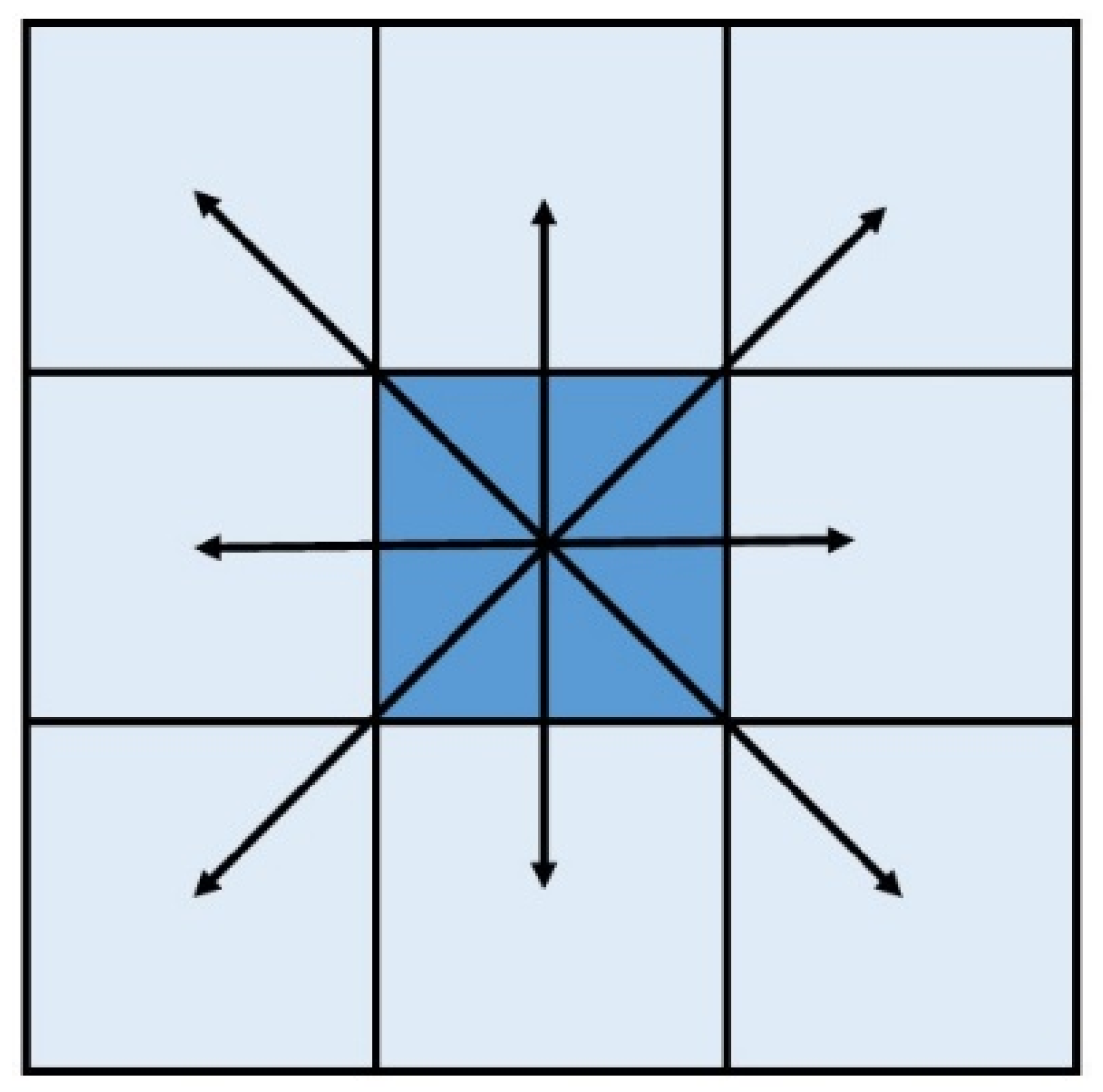
The flow direction mainly refers to the direction of the flow away from the cell. The D8 [27] algorithm is generally used in ARCGIS, which needs to calculate the weight difference between the center cell and the maximum distance to determine the target cell. In the layout structure of 3, let the central cell be Zc, and its flow direction is selected in its 8 neighbor cells Zi (i = 1, 2, …, 8) according to certain judgment conditions; the judgment condition is:
k = 1 when Zi is in the east–west or north–south direction, k = 1√2 when Zi is in the diagonal direction, and it is assumed that the flow of the central cell Zc flows to all Zi, that is, the flow of the central cell flows to all the neighbor cells in the steepest direction. Each time the flow of the central cell can only flow in one direction of the neighboring cells; when there are multiple neighboring cells with equal weight difference, a direction is randomly selected as the flow direction. Figure 1 is the flow direction diagram of the central cell.
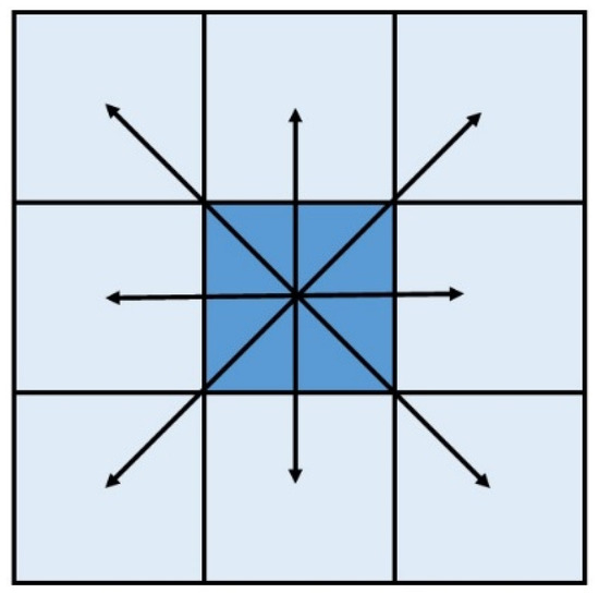
Figure 1.
Cell flow direction.
- Water Allocation Rules
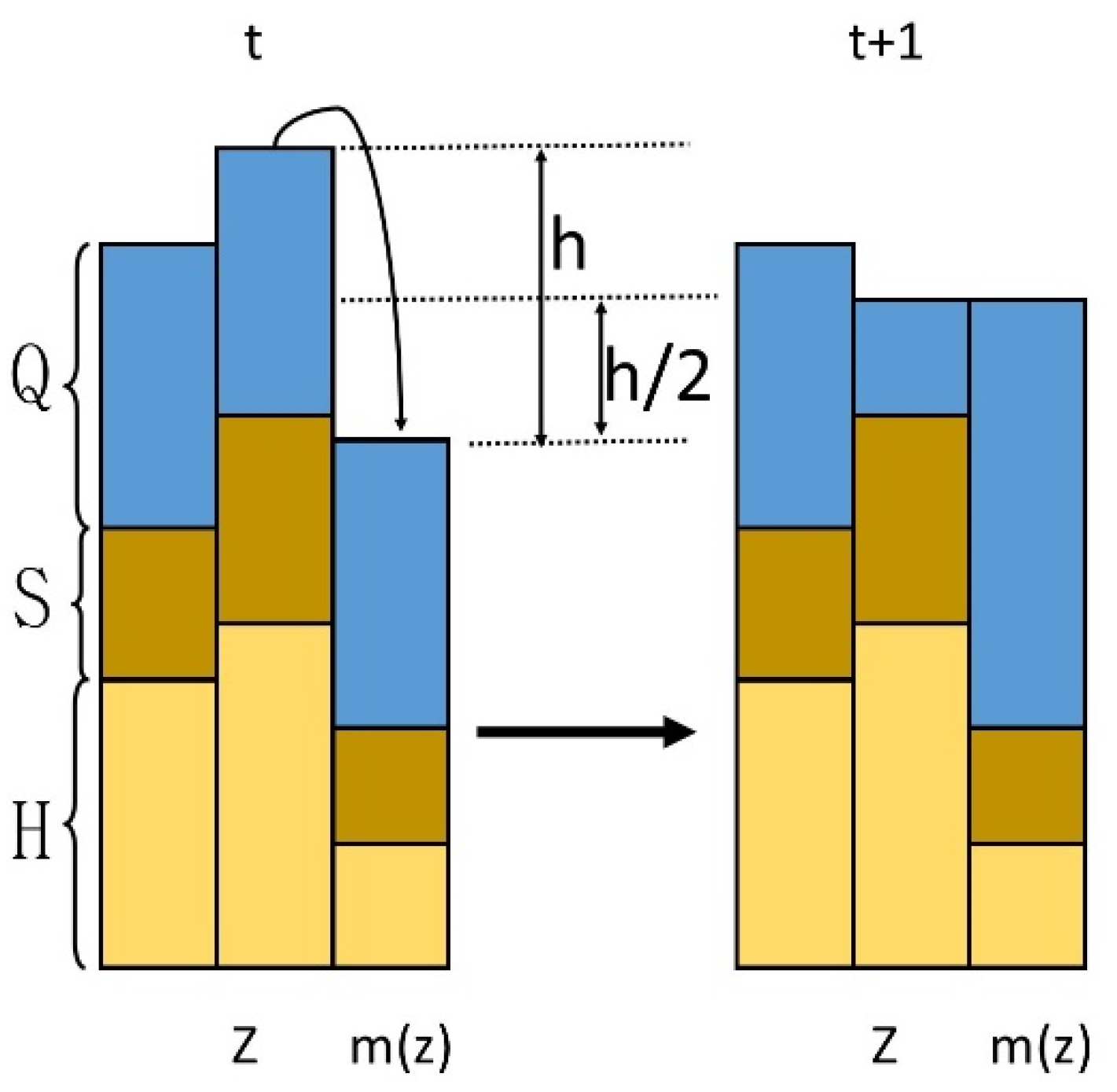
The water flow of the central cell Z flows to the smallest cell M (z) in the neighboring cell. Figure 2 is a schematic diagram of the amount of water exchanged between cells.

Figure 2.
Allocation on cells.
The amount of water exchanged between cells depends on the following equation [17]:
where, Hz is the center cell height, mm; Sz is the center cellular sediment height, mm; Qz is the water depth of the center cell, mm; Hm (z) represents the elevation of the neighbor cell with the smallest water head, mm; Sm(z) represents the sediment height of the neighbor cell with the smallest head of water; and Qm(z) represents the water depth of the neighbor cell with the smallest head, mm.
The water depth in the center cell z at time t + 1 and the smallest neighbor cell at location water head can be expressed as:
The water in the current cell at time t is calculated by a continuous equilibrium equation:
In the formula, Q is the amount of water in the current cell; t is time; Qi is the amount of water entering the current cell; Q0 is the amount of water flowing out of the current cell.
Among them, Qi includes the sum of rainfall and the amount of water flowing from adjacent cells into the current cell, and Q0 includes the amount of soil infiltration and the amount of water flowing into the smallest neighbor cells at the water head.
- Calculation Rules of Flow Rate
The flow velocity of this model adopts Manning formula:
where V is flow rate, mm/min; h is the water level difference between the center cell and the smallest neighbor cell with the head of water, mm; S is the hydraulic slope and the sine value of the slope; and n is the roughness coefficient of the slope.
- Rules of Erosion Transport and Deposition
Rules of erosion, sediment transport, and deposition of each cell: Erosion occurs when the runoff sediment transport capacity of the cell is greater than the runoff sediment concentration and the flow shear stress is greater than the critical shear stress of the soil. Sediment transport when the runoff sand transport capacity on the cellular is greater than the runoff sand content, but the flow shear stress is less than the critical soil shear stress. Sedimentation occurs when the sediment transport capacity of cellular runoff is less than the sediment concentration of runoff.
This model is calculated by the following formula [28]:
In the formula, Dr is the erosion rate, kg/(m2·s); Kr is the erosion coefficient, kg/(N·s); τ is runoff shear stress, N·m2; τc is soil critical shear stress, N·m2; q is single width flow, m2/s; c is sediment content, kg/m3; and Tc is runoff transport capacity, kg/(m·s).
In the formula, ρ is the bulk density of water, g·cm−3; g is the acceleration of gravity, m2·s−2; R is the hydraulic radius which can be approximated by the water depth in each cell; and S is the hydraulic slope, taking the sine slope.
Runoff sediment concentration using Zhang Keli and other research results [29]:
In the formula, c is runoff sediment content, kg/m3; Q is runoff, mL/s; J is slope.
3. Results
Five groups of experiments were conducted by setting five different slopes (5°, 10°, 15°, 20°, 25°). During the tests, the slope erosion morphology was scanned by a three-dimensional laser scanner. The three-dimensional laser scanner was used to scan the surface before rainfall, and the DEM data obtained was recorded as A0. Then, an artificial simulation of rainfall was carried out and lasted for 1 h. After the rainfall, no water was left on the surface of the soil trough, and the DEM data obtained by scanning the surface again was recorded as A1. Geomagic studio software was used to denoise and splice the scanned DEM data of the soil groove, so as to obtain the complete DEM data of the slope under the same coordinate system after removing the invalid points. Then, ArcGIS software was used to compare scanning result A1 after rainfall with the initial scanning result A0 to obtain the DEM data of the coordinate elevation difference of each point on the slope. At the same time, ArcGIS software was used to extract the rill network, derive the depth data of each rill, and extract the plane area of each rill.
3.1. The Influence of Slope on the Yield Rate
Figure 3 shows that in the early stage of rainfall, most of the raindrops that fell on the slope surface infiltrated into the soil through the soil pores and transformed into soil moisture. Therefore, the degree of aggregation of rainwater on the slope surface was weak and the runoff rate was less. With the progress of the rainfall, the soil was gradually saturated with moisture, and the soil moisture infiltration capacity gradually weakened. The infiltration and runoff process reached a relative balance, and the runoff yield began to stabilize. When the slope increased from 5° to 15°, the average flow rate increased, and when it continued to increase, the average flow rate began to decrease. Therefore, when the slope ranges from 15° to 20°, there may be a critical value, and for the slope in the critical state, the average runoff yield reaches a high level.
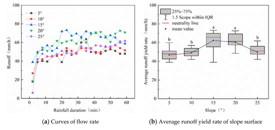
Figure 3.
The influence of different slopes on the yield rate.
3.2. The Influence of Slope on Sediment Yield
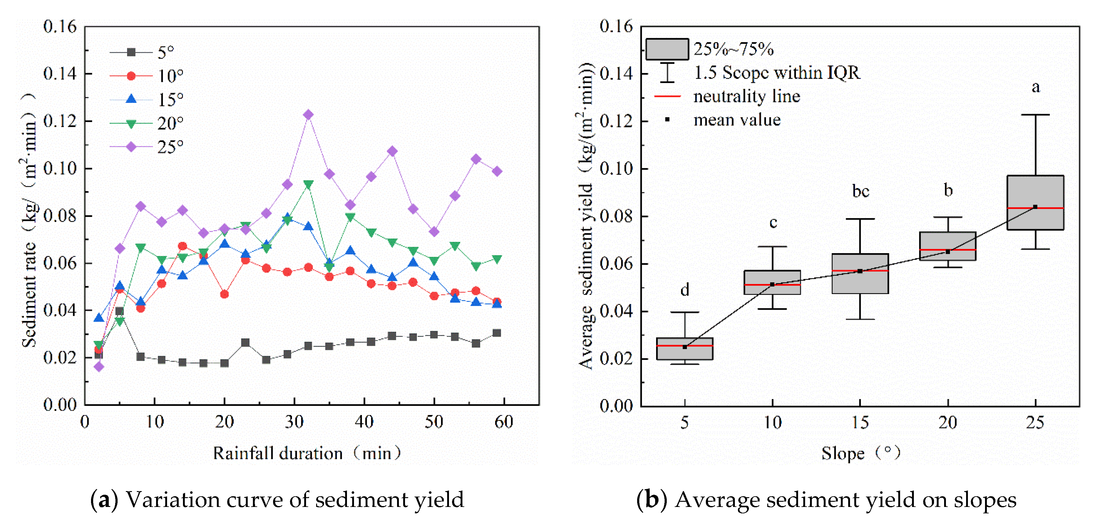
It can be seen from Figure 4 that the sediment yield rate obviously fluctuates on slopes with different gradients during rainfall. Especially on the 25° slope, the maximum fluctuation amplitude exceeded 34.6%, and there was no stable trend until the end of the rainfall. From the beginning to the end of the rainfall, the sediment yield curve was a process of fluctuating rises, and the increasing trend weakened gradually. The sediment yield on slopes with different gradients increased to varying degrees; the increase in sediment yield on the slope with 5° gradient was not obvious, and the trend was relatively flat. When the slope increased, the fluctuation in sediment yield gradually became obvious. The sediment yield on the 25° slope increased rapidly at the beginning of the rainfall, and the growth trend weakened at about 10 min. However, in the middle and late period of rainfall, after 30 min, it began to fluctuate significantly until the end of the rainfall, which was quite different from the variation in sediment yield the on 5° and 10° slopes. The increase in slope made the soil unstable and prone to collapse and gravity erosion under the scouring water flow, and the collapsed soil blocked an increase in sediment yield.
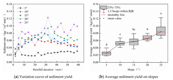
Figure 4.
Effect of different slope gradients on sediment yield.
The variation law of average sediment yield on bare land slopes is similar to that on grassland slopes, and the average sediment yield shows a linear growth trend with increases in slope gradient. With the increase of slope gradient, the gravity along the direction of the slope also increases. Under the action of gravity, soil particles splashed by rainfall are more likely to be transported and moved by runoff, and it is difficult to settle on the slope. Therefore, loose soil particles on the slope will flow off of the slope to a greater extent with runoff. On the other hand, the slope gradient is closely related to the flow conditions. An increase in slope gradient also enhances the shear effect of flow on the slope. Under the same flow conditions, more surface sediment is subject to erosion, which increases the sediment yield rate.
3.3. Erosion Patterns of Bare Black Soil Slopes under Different Gradients
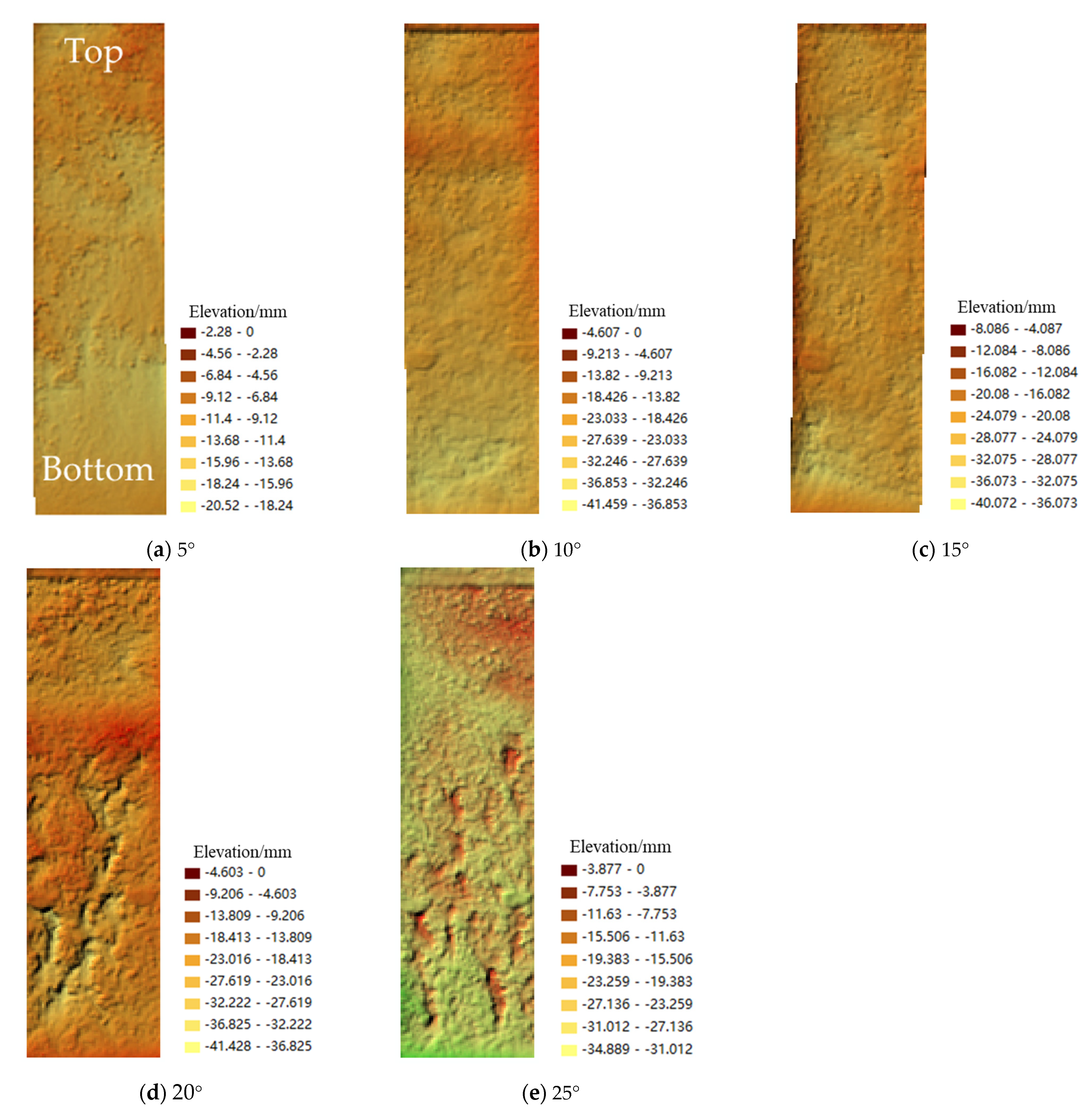
It can be seen from Figure 5 that the erosion morphology of the 5° slope was mainly characterized by sheet erosion, accompanied by splash erosion, and scale pits caused by raindrops can be observed in the slope area. The pit on the top of the slope was serious, and the bottom of the slope was relatively smooth and flat, indicating that the degree of water flow convergence on the top of the slope was weak. The erosion mode was mainly the splash erosion caused by raindrops, and the flow at the bottom of the slope was relatively sufficient and mainly affected by runoff erosion. Runoff is the main driving force of rainfall erosion, and erosion will be more serious in areas with larger runoff. The erosion area was mainly concentrated in the middle and lower parts of the slope, and the average erosion depth was 13.54 mm. Through extraction of the areas with serious slope erosion (erosion depth ≥1.5 cm), it was found that the surface area of the area with serious slope erosion at 5° was 0.087 m2, accounting for 14.5% of the total slope area. With the convergence of water flow, the flow condition was enhanced, and the confluence area gradually increased. When the flow reached the bottom of the slope, the erosion capacity of runoff on the slope reached its maximum, so the erosion area at the bottom of the slope was larger than that in the middle of the slope, and the sheet erosion phenomenon was more obvious. When the slope gradient increased to 10°, the pit depression on the slope was weakened, and the dominant erosion mode was mainly sheet erosion, which masked the influence of raindrop splash erosion on slope morphology. The slope bottom was obviously affected by sheet erosion, and a relatively depressed terrain appeared. The erosion area was mainly concentrated at the bottom of the slope, and the average erosion depth was 16.92 mm. Through the extraction of areas with serious slope erosion, it was found that the surface area of areas with serious slope erosion at 10° was 0.105 m2, accounting for 17.5% of the total slope area. Compared to the 5° slope, the erosion area was closer to the outlet, indicating that with the increase in gradient, the kinetic energy of the flow at the bottom of the slope increased, and the erosion process on the topography at the bottom of the slope was more intense. The erosion morphology of the 15° slope was not significantly different from that of the 5° and 10° slopes, but the upper and middle parts of the slope also began to show the characteristics of sheet erosion, indicating that with the increase in gradient, the runoff scouring ability on different areas on the slope was increased. The erosion was mainly concentrated in the upper and bottom areas of the slope, and the average erosion depth was 19.97 mm. Through the extraction of the areas with serious slope erosion, it was found that the surface area of the area with serious slope erosion at 15° was 0.106 m2, accounting for 17.7% of the total slope area. There were some small scale pits on the slope that had a certain erosion depth and the potential for fall ridge development. It can be seen from Fig. 5 (d) that the erosion morphology of the 20° slope was quite different from that of the previous slopes, and the slope had obvious drop-sill characteristics. The erosion force of runoff in the vertical direction was relatively large, and the flow continued to cut and erode under this convergence, which made it evolve into the lower gully head and show a trend of tracing toward the source and extending upward. Erosion area distribution was uniform but mainly concentrated in the lower part of the slope; the average erosion depth was 19.86 mm. Through the extraction of areas with serious slope erosion, it was found in Figure 6 that the surface area of these areas at 20° gradient was 0.139 m2, accounting for 23.2% of the total slope area. However, with continued increases in the slope gradient, the erosion pattern did not change significantly. The difference was that the development of the fall ridge was more slender, which may be related to the increase in slope gradient. The flow velocity increased, the flow kinetic energy increased, and the local scouring effect was more intense. The distribution of the erosion area was relatively uniform, and the average erosion depth was 20.12 mm. By extracting the areas with serious slope erosion, it was found that their surface area at the 25° gradient was 0.170 m2, accounting for 28.3% of the total slope area. An erosion area with a large catchment area appeared at the top of the slope. In contrast to the erosion characteristics of the middle and lower parts of the slope, the erosion area of the slope was contiguous and showed obvious sheet erosion characteristics.
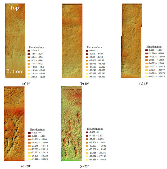
Figure 5.
Morphological characteristics of slope erosion under different slope gradients.
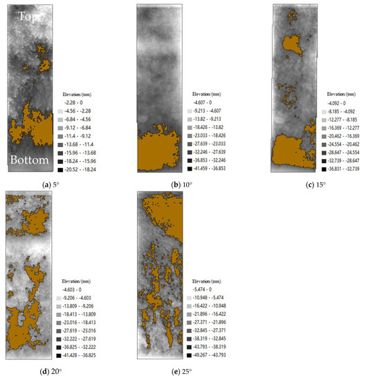
Figure 6.
Severe areas of slope erosion under different slope gradients.
3.4. Confluence Path Development Process
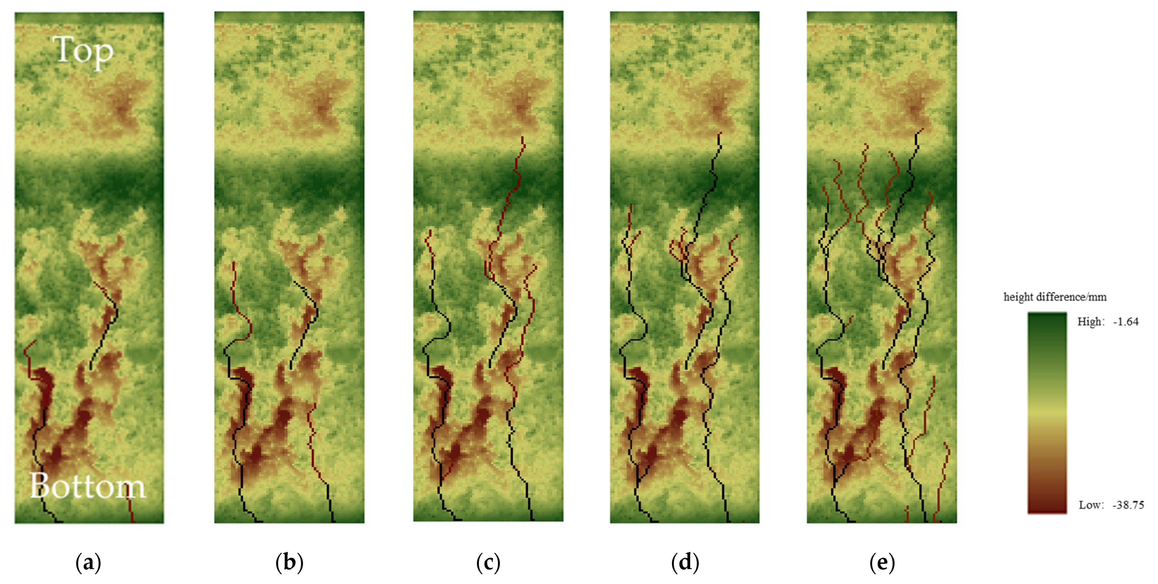
Taking the 20° slope as an example, we studied the confluence path development process. The confluence accumulation was calculated based on the flow direction data. By setting different thresholds, the confluence paths of different confluence accumulations could be extracted. The flow tended to converge from the high to the low, so the closer to the bottom of the slope, the greater the cumulative flow, and the higher the degree of convergence. Setting different cascading cumulative flows from large to small could reflect the derivation and development of the confluence path. Slope runoff was the main driving force of rainfall erosion. The larger the accumulated confluence, the more serious the erosion became, and it was easier to form slope topography such as fall ridges, which provide a universal indication that the development of a confluence path can reflect the development of erosion. First of all, it can be seen in Figure 7a that the flow with a large accumulated confluence mainly occurred near the bottom of the slope, the erosion around the confluence path was relatively serious, and the erosion depth was mostly above 25 mm. The gully erosion at the bottom of the slope was affected by runoff erosion. The channel terrain was relatively low, and the flow easily sank and converged here, which made the accumulated confluence larger. The confluence path in Figure 7b began to show the trend of traceability, extending along the area with deep erosion to the middle of the slope, and extending from the slope area with erosion depth of about 25 mm to the slope area with an erosion depth of about 18 mm. It can be seen from Figure 7c that the confluence path on the slope had developed three water flows with certain conditions, and the water flow further extended to the top of the slope, and there was a trend of bifurcation to form tributaries. It can be seen from Figure 7d that the branched tributaries also began to gradually extend, and the flow length increased, slowly covering the slope area with an erosion depth of about 10 mm. The confluence path in Figure 7e was fully developed. It can be seen that the distribution of the river network on the slope surface was roughly shown. The closer to the top of the slope, the denser the tributaries covered and extended to the area where the erosion was not very deep. Slope erosion is a process of retrogressive erosion, which gradually extends from the bottom of the slope to the top, and gradually develops from the dropper to the lower gully head and then to the shallow gully. Similarly to the evolution and development of erosion, the confluence path extends from the bottom of the slope to the top of the slope, and extends from the slope area with serious erosion to the slope area with small erosion depth. Therefore, by drawing the confluence path of water flow (the black paths in the figure represent the main sink paths, and the red paths represent the branch sink paths), we could roughly predict the trend of erosion occurrence and development, and thus concluded that the erosion caused by rainfall on the slope is a process of steady development and continuous strengthening.
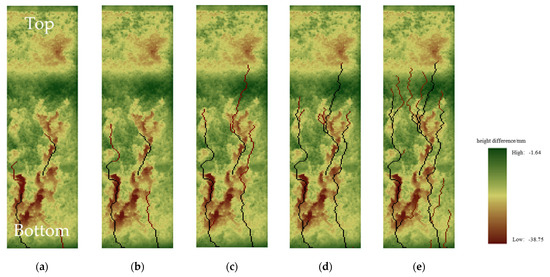
Figure 7.
Development process of the confluence path. (a–e) represents the converging paths at different moments.
4. Discussion
4.1. Effect of Slope on Runoff Erosion
It can be seen from Figure 8, with increases in gradient, runoff increases first and then decreases. The runoff reaches a maximum at 20°, and then begins to decrease as the slope gradient continues to increase. The runoff on the slope is affected by gravity and rainfall. When the slope gradient is small, gravity plays a leading role. The greater the slope gradient, the less rain landing on the slope is converted into infiltration water. Under the action of gravity, the water more easily converges on the slope to form runoff, and the runoff increases. When the slope gradient is large, rainfall plays a leading role. The increase in gradient causes the rainfall area on the slope to decrease, the rainfall that falls on the slope under the same rainfall intensity decreases, and the runoff decreases.
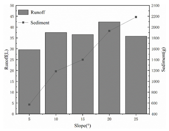
Figure 8.
Runoff erosion under different slope gradients.
The amount of erosion increases with increases in the gradient, showing a linear growth trend. On the one hand, due to the increase in slope gradient and flow conditions, runoff can erode and transport more sediment, and erosion increases in the process of continuous accumulation. On the other hand, it is caused by the stability of the slope itself. The greater the slope gradient, the more unstable the slope soil. Coupled with the scouring effect of water flow, the possibility of collapse and gravity erosion on the slope is increased, and the erosion amount is increased.
4.2. Validation of the Model in Black Soil Area
This experiment verified the realization model of slope runoff and sediment yield caused by each rainfall under different rainfall intensity conditions on the same slope. The parameters adopted in the model are shown in Table 2:
where Q0 is the measured value, Q is the measured average value, Qp is the simulated value, and n is the number of measured values.

Table 2.
Parameter values of black soil test model.
4.3. Validation of Model Production Process
The process of runoff and sediment production involves complex water and sediment exchange and is affected and limited by many factors (rainfall intensity, topography, soil, pre-soil moisture content, microtopography, etc.). The exploration of this process has always been a hot topic in the field of erosion model research. It can be seen through Figure 9, under a rainfall intensity of 30 mm/h, the runoff yield process expressed by the model was roughly the same as the measured runoff yield curve in the trend, and there was no obvious fluctuation feature in the rainfall duration. In the middle and late rainfall period, the simulated value was slightly larger than the experimental value, but the difference was not significant. Under a rainfall intensity of 50 mm/h, the simulated and experimental runoff yield trends were also quite different, and the runoff yield curve was relatively flat without an obvious upward trend. However, it is worth noting that from the early to late stages of rainfall, the simulated value was higher than the experimental value in most rainfall durations. The possible reason is that when the rainfall intensity of 50 mm/h was simulated, the infiltration rate under the first group of conditions was still used, and in the process of refilling the slope, the actual infiltration rate of the slope was different, which led to a differential expression of the simulation results. Under the rainfall intensity of 70 mm/h, the simulated and experimental flow rate trends were slightly different. The flow rate simulated by the model was still flat, while the measured flow rate showed a trend of rapid increase and gradual decrease in the initial stage of rainfall, and the fluctuation characteristics were obvious. A reasonable explanation is that the raindrop impact will disturb the runoff generation process on the slope; however, the disturbance process involves mechanism research, and there are difficulties to be overcome. The specific impact needs to be further supported by theoretical research. Therefore, the current model is still unable to better simulate the real-time runoff generation process on a slope under heavy rainfall intensity. It is necessary to take into account the impact of raindrops and increase the constraint conditions to render the simulation effect more realistic and effective.


Figure 9.
Comparison between measured and simulated runoff rates under different rainfall intensities.
When the rainfall intensity was 30 mm/h, 50 mm/h, and 70 mm/h, the Ens coefficient was calculated by Formula (6) as 0.87, 0.97, and 0.70, respectively. It can be seen that the rainfall intensity of 50 mm/h yielded the largest Ens coefficient and the best model of the runoff simulation process.
4.4. Verification of Sediment Production Process of the Model
It can be seen from Figure 10 that under the rainfall intensity of 30 mm/h, the mid-term experimental value was slightly larger than the simulated value. With continuous rainfall, the simulated value became larger than the experimental value after 32 min. The possible reason is that the soil erosion resistance will gradually change with the increase in soil water content. In the model, the critical shear stress of soil is a constant value for the entire rainfall duration. The difference in anti-corrosion ability accounts for the difference between the simulated and measured results. It is worth noting that the measured sediment yield curve had a different increment in the early stage of rainfall, while the simulated sediment yield curve was relatively flat, and there were no obvious fluctuation characteristics. The actual slope may have different degrees of soil compaction in different regions, resulting in differences in rill erosion resistance. In the process of fighting against runoff erosion, a distinctly strong and weak zone is formed, so the sediment yield rate shows certain fluctuation characteristics. In terms of the model, the degree of soil compaction in different regions of the slope is consistent and there is no difference. Therefore, the calculation is strictly in accordance with the rules, the generation of special situations is expected, and the sediment production process is relatively stable. Under the rainfall intensity of 50 mm/h, the simulation value of sediment yield in the early stage of rainfall was less than the experimental value, because the main process of slope erosion caused by early rainfall was splash erosion. A large number of loose soil particles were formed by the impact of raindrops and transported to the bottom of the slope with the flow. The model assumes that rill erosion is mainly caused by runoff erosion, that is, the slope water depth is the main driving force for rill erosion, and the splash erosion effect is not considered. Under the rainfall intensity of 70 mm/h, the number of raindrops per unit time on the slope increased, the soil structure was continuously disturbed, it was difficult to maintain stability, the fluctuation of the sediment yield rate was relatively strong, and the data were not representative, so it was not analyzed.

Figure 10.
Comparison between measured and simulated sediment rates under different rainfall intensities.
When the rainfall intensity was 30 mm/h, 50 mm/h, and 70 mm/h, the Ens coefficient was calculated with Formula (6) as 0.52, 0.27, and 0.02, respectively. When the rainfall intensity was 30 mm/h, the Ens coefficient of the model yielded the best sand production simulation process, while when the rainfall intensity was 50 mm/h or 70 mm/h, the Ens coefficient of the model was lower than 0.5, and the validity of the model was poor.
4.5. Verification of Total Yield and Sediment Yield of the Model
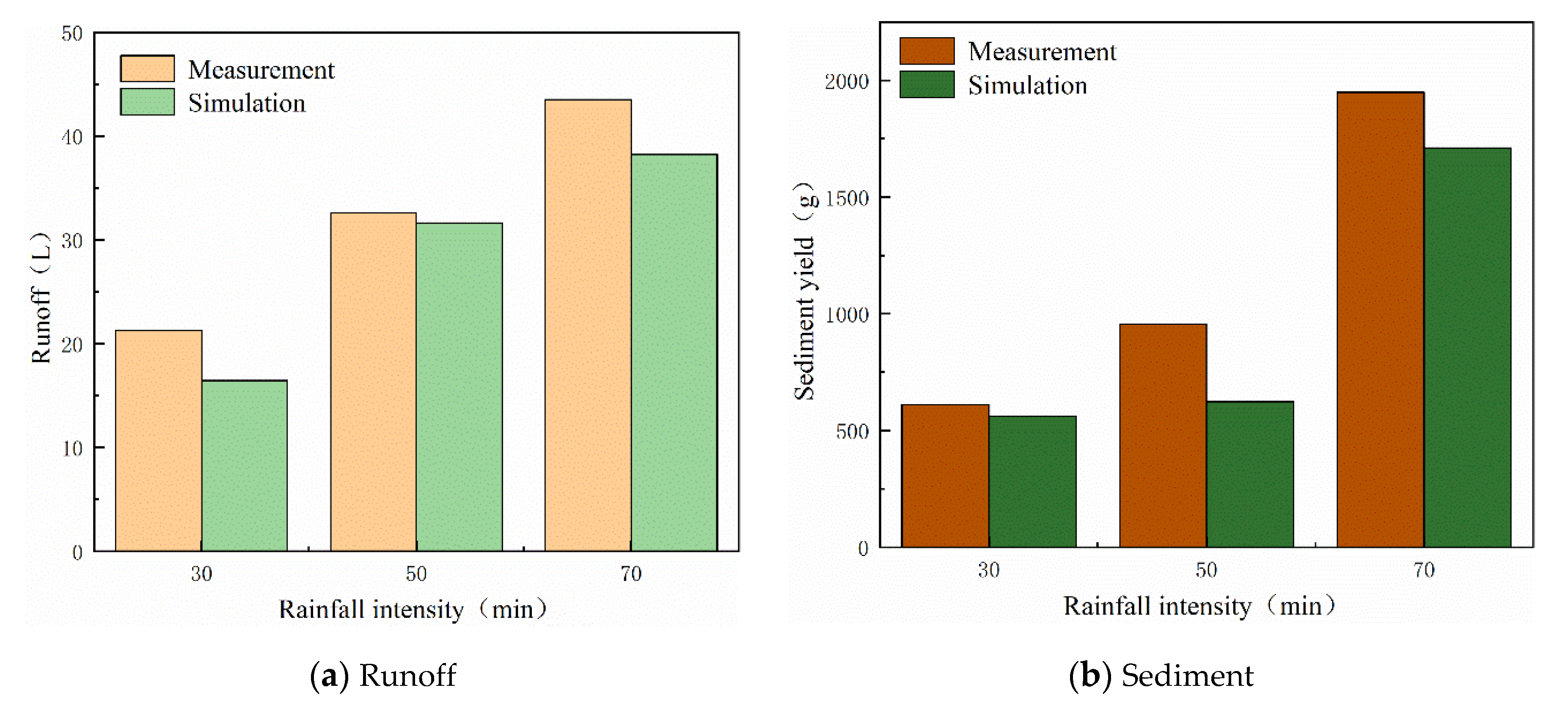
It can be seen from Figure 11a that under different rainfall intensities, the simulation values were smaller than the experimental values, and the error coefficient was between 5.6% and 22.6%. Among them, the model yielded the best simulation effect on runoff under 50 mm/h rainfall intensity, and the error coefficient was 5.6%. As the rainfall intensity continues to increase, the error coefficient increased to 12.1%. The possible explanation is that the increase in rainfall intensity intensified the turbulence of runoff, resulting in more runoff. In the actual rainfall process, raindrops have a disturbance effect on runoff. The raindrop strike will accelerate the formation of crust on the slope, and the surface soil becomes relatively dense, which delays water infiltration on the slope, and rainfall is more likely to converge on the slope to form runoff. Crust formation affects soil erosion by raindrop-impacted flow through changing particle size and cohesion between particles on the soil surface, as well as surface microtopography. Therefore, changes in soil microtopography can, in theory, be employed as a proxy to reflect the complex and dynamic interactions between crust formation and erosion caused by raindrop-impacted flow. However, there are no qualitative explanations for the small changes in soil topography [31]. The model cannot simulate the influence of raindrop impact on the infiltration capacity caused by the formation of crust on the slope surface, so the simulated runoff is less than the experimental value, and the error coefficient increases. From Figure 9(b1,b2), under different rainfall intensities, the error coefficients were between 8.1% and 32.4%, and the experimental values were greater than the simulation values. It should be noted that under the continuous impact of raindrops, soil will be disturbed and soil particles become loose and are more easily separated and transported, so that the amount of erosion shows some difference. In general, the model can effectively predict the amount of runoff erosion on the slope under each rainfall, roughly predict the degree of erosion damage on the slope, and provide support for further erosion prevention and control work.
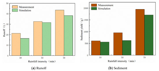
Figure 11.
Total runoff and total sediment yield under different rainfall intensities.
4.6. Validation on Runoff Model in Loess Area
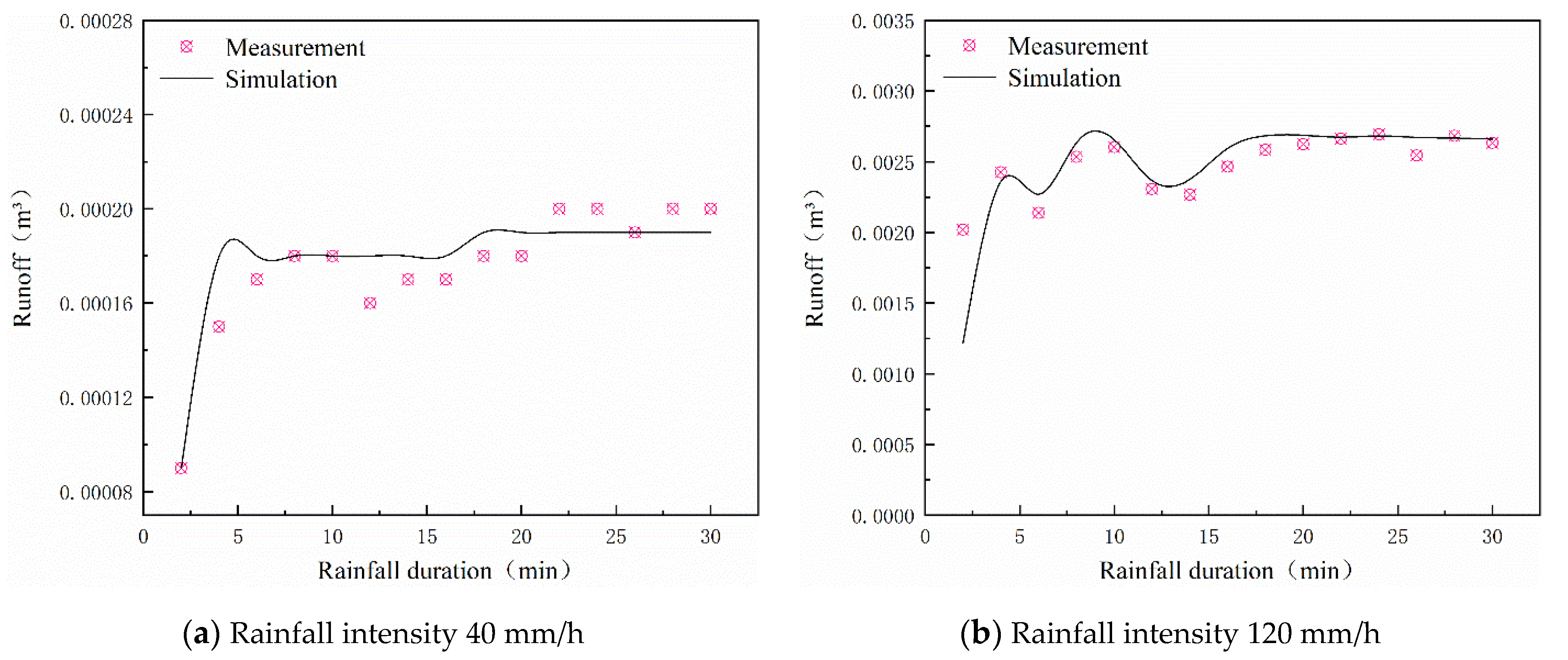
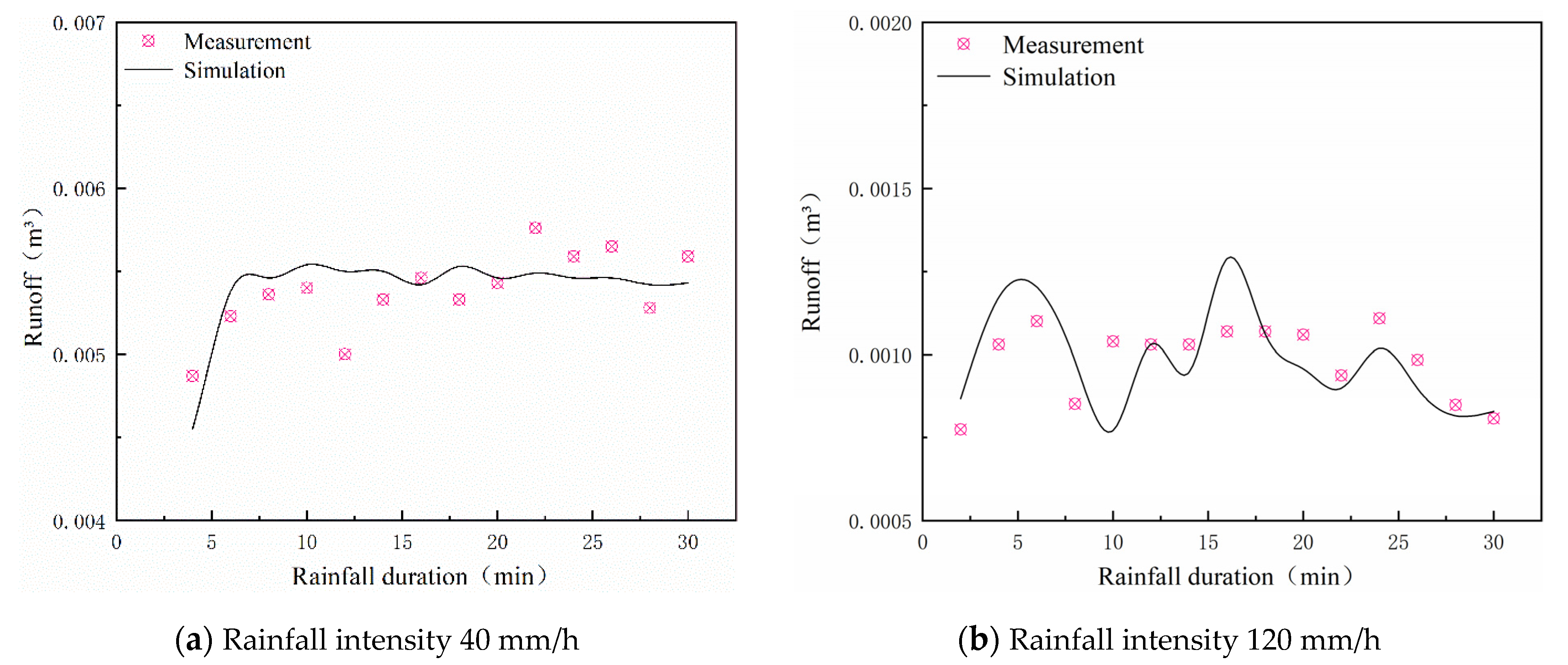
Figure 12 and Figure 13 show the data comparison between simulated and measured values of cellular automata applied to loess. By calculating the error coefficient between the tested and simulated values of the loess slope with a slope of 2 m, the maximum Re was 5.8% when the rain intensity was 40 mm/h, and the minimum was 0. When the slope length was 3 m and the rain intensity was 40 mm/h, the maximum Re was 6.5% and the minimum was 0.5%; when the rain intensity was 120 mm/h, the maximum Re was 9.5% and the minimum was 0, which proves that the cellular automata model is also applicable in the loess area, thus verifying the validity of the model.
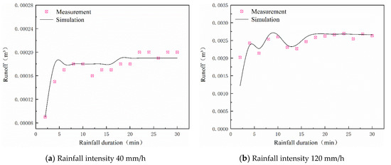
Figure 12.
Comparison between measured and simulated runoff rates under different rainfall intensities (loess test steel trough is 2 m).
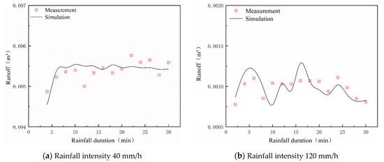
Figure 13.
Comparison between measured and simulated runoff rates under different rainfall intensities (loess test steel trough is 3 m).
4.7. Analysis of Slope Erosion Morphology Development Process
In order to more deeply study the development process of slope erosion morphology, the simulation data generated by the model were used to analyze the development process of slope erosion morphology under the same slope with different rainfall intensities.
It can be seen from Figure 14 that when the rainfall intensity was 30 mm/h, the slope erosion pattern was mainly gully erosion; when the rainfall intensity was 50 mm/h, the slope erosion pattern consisted of both groove erosion and surface erosion; and when the rainfall intensity was 70 mm/h, the erosion pattern on the slope was mainly surface erosion.
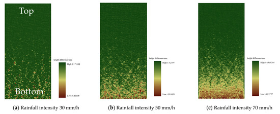
Figure 14.
Slope erosion patterns under different rainfall intensity conditions.
By comparing the experimental values generated by artificial rainfall with those simulated by the rill erosion model based on cellular automata, it was concluded that the simulated conditions of the model were close to the actual sediment yield. Therefore, the simulated values generated by the model were used to simulate and predict the morphology of soil slope erosion using Arcgis technology. Figure 14 shows predicted slope erosion patterns under different rainfall intensity conditions.
The rill erosion model based on cellular automata could not only simulate the erosion process and slope morphology, but also analyze the characteristic parameters of slope erosion. Table 3 shows the extraction results for characteristic parameters of slope erosion.

Table 3.
Parameter values of black soil test model.
With increases in rainfall intensity, slope erosion parameters such as maximum erosion gully length, depth, and density also increase, and characteristic parameters such as slope erosion gradually become more serious. When the rainfall intensity is 70 mm/h, because the slope erosion form is mainly surface erosion, the ditch length, ditch depth and ditch width under the condition of feature parameters were not extracted.
4.8. Limitations and Future Work Prospects
(1) At present, much work has been done at home and abroad on the simulation and prediction of the spatial and temporal dynamics of the erosion and sand production process in watersheds, but the empirical formulae and empirical coefficients used in the models built by the CA method at this stage are mainly oriented to loess areas. The applicability of the model to black soil areas, where there are differences in soil properties, needs to be verified. The topographic data input into the model are for a simulated slope based on slope dimensions that have some deviation from actual slope topography. Therefore, only the erosion patterns of a slope after rainfall are predicted rationally, and the results of the model run are not compared with real erosion patterns. In the later stage, 3D scanning of the slope topography can be carried out before the artificial simulation rainfall tests, and the scanned data can be used as input parameters of the model to increase the realism and reliability of the simulation results.
(2) The hydrodynamic erosion and sand production model for black soil areas established on the basis of experimental conditions only takes into account the effect of runoff scour. In the actual rainfall process, the influence of raindrop impact cannot be ignored. Therefore, the model can be improved by adding the characteristic parameters of raindrops in the subsequent study.
5. Conclusions
The research focus of this paper was on the slope erosion process in black soil areas. Applying the theory and methodology of cellular automata, combined with the principles of hydraulics and rill erosion, a slope rill erosion model based on cellular automata was constructed. The artificial rainfall experiment was used to study the occurrence, development, and evolution of slope erosion under different rainfall intensities on the same slope; at the same time, the actual values generated by the artificial rainfall experiment were compared with the simulated values based on the cellular automata model to verify the effectiveness of the rill erosion model.
(1) Through the analysis of slope erosion morphology after rainfall, it was confirmed that with increases in slope gradient, the surface area and average erosion depth of the area with serious slope erosion gradually increased, the flow conditions were enhanced, and the fulcrums of flow convergence gradually increased. Fish scale-shaped eroded areas such as ridges and pits begin to appear in different regions of the slope.
(2) The slope rill erosion model based on cellular automata was used to simulate erosion by designing a cell space, cell state, neighbor cells, and conversion rules. The model has a simple structure and involves fewer parameters, which reduces the cumbersome steps in the calculation process.
(3) The simulated values generated by inputting the experimental parameters through the CA model were compared with the experimental values generated by artificial rainfall, and the Nash–Sutcliffe coefficient and error coefficient were calculated. The three runoff processes with different rainfall intensities were all greater than 0.5, indicating that the simulation effect of the runoff process was better; the coefficients of the three sediment production processes with different rainfall intensities were all lower than 0.5 except for the 30 mm/h rain intensity, indicating that the simulation of the sediment production process did not achieve the optimal effect and needs further study.
(4) The cellular automata slope rill erosion model could fully demonstrate the development process of slope erosion. When the rainfall intensity was small, the erosion form was mainly dominated by gully erosion. As the rainfall intensity gradually increased, the erosion intensity gradually increased. Gully erosion was converted to surface erosion; from a simulated rainfall, it can be seen that the erosion of the slope was mainly concentrated at the bottom of the slope at the beginning of the rainfall. As time passed, the erosion gradually formed rills upward. As the rainfall intensity increased, the length, width, and erosion intensity of the rills also increased.
Author Contributions
Conceptualization, S.L. and Y.H.; data curation, Q.L.; formal analysis, S.L.; funding acquisition, Y.H.; software, Q.L. and J.C.; supervision, Y.H.; validation, S.L. and Q.L.; writing—original draft, S.L.; writing—review and editing, J.C. and Y.H. All authors have read and agreed to the published version of the manuscript.
Funding
This research was funded by the National Natural Science Foundation of China, grant number 51979275, and National Key R&D Program of China, grant number 2017YFC0404402, and National Natural Science Foundation of China, grant number 51809106, and the Open Research Fund of State Key Laboratory of Information Engineering in Surveying, Map-ping and Remote Sensing, Wuhan University, grant number No. 19R06.
Acknowledgments
This work was supported by the National Natural Science Foundation of China; National Key R&D Program of China; National Natural Science Foundation of China; the Open Research Fund of State Key Laboratory of Information Engineering in Surveying, Mapping and Remote Sensing, Wuhan University. The experimental site was provided by the Heilongjiang Academy of Water Sciences.
Conflicts of Interest
The authors declare no conflict of interest.
References
- Yang, X.M.; Zhang, X.P.; Deng, W.; Fang, H.J. Black soil degradation by rainfall erosion in Jilin, China. Land Degrad. Dev. 2003, 14, 409–420. [Google Scholar] [CrossRef]
- Yin, L.; Zhang, B.; Pan, X.; Shi, D. Current status and comprehensive control strategies of soil erosion for hilly region in the Southern China. Sci. Soil Water Conserv. 2008, 6, 22–27. [Google Scholar]
- Welch, R.; Jordan, T.R.; Thomas, A.W. A photogrammetric technique for measuring soil-erosion. J. Soil Water Conserv. 1984, 39, 191–194. [Google Scholar]
- Dymond, J.R.; Hicks, D.L. Steepland erosion measured from historical aerial photographs. J. Soil Water Conserv. 1986, 41, 252–255. [Google Scholar]
- Gessesse, G.D.; Fuchs, H.; Mansberger, R.; Klik, A.; Rieke-Zapp, D.H. Assessment of Erosion, Deposition and Rill Development on Irregular Soil Surfaces Using Close Range Digital Photogrammetry. Photogramm. Rec. 2010, 25, 299–318. [Google Scholar] [CrossRef]
- Cook, K.L. An evaluation of the effectiveness of low-cost UAVs and structure from motion for geomorphic change detection. Geomorphology 2017, 278, 195–208. [Google Scholar] [CrossRef]
- Vinci, A.; Todisco, F.; Brigante, R.; Mannocchi, F.; Radicioni, F. A smartphone camera for the structure from motion reconstruction for measuring soil surface variations and soil loss due to erosion. Hydrol. Res. 2017, 48, 673–685. [Google Scholar] [CrossRef]
- Milan, D.J.; Heritage, G.L.; Hetherington, D. Application of a 3D laser scanner in the assessment of erosion and deposition volumes and channel change in a proglacial river. Earth Surf. Process. Landf. 2007, 32, 1657–1674. [Google Scholar] [CrossRef]
- Eitel, J.U.H.; Williams, C.J.; Vierling, L.A.; Al-Hamdan, O.Z.; Pierson, F.B. Suitability of terrestrial laser scanning for studying surface roughness effects on concentrated flow erosion processes in rangelands. Catena 2011, 87, 398–407. [Google Scholar] [CrossRef]
- Bremer, M.; Sass, O. Combining airborne and terrestrial laser scanning for quantifying erosion and deposition by a debris flow event. Geomorphology 2012, 138, 49–60. [Google Scholar] [CrossRef]
- Smith, R. The application of cellular automata to the erosion of landforms. Earth Surf. Process. Landf. 1991, 16, 273–281. [Google Scholar] [CrossRef]
- Murray, A.B.; Paola, C. A cellular-model of braided rivers. Nature 1994, 371, 54–57. [Google Scholar] [CrossRef]
- Pilotti, M.; Menduni, G. Application of lattice gas techniques to the study of sediment erosion and transport caused by laminar sheetflow. Earth Surf. Process. Landf. 1997, 22, 885–893. [Google Scholar] [CrossRef]
- D’Ambrosio, D.; Di Gregorio, S.; Gabriele, S.; Gaudio, R. A cellular automats model for soil erosion by water. Phys. Chem. Earth Part B-Hydrol. Ocean. Atmos. 2001, 26, 33–39. [Google Scholar] [CrossRef]
- Wei, L. LANDSAP: A coupled surface and subsurface cellular automata model for landform simulation. Comput. Geosci. 2001, 27, 363–367. [Google Scholar] [CrossRef]
- Bursik, M.; Martinez-Hackert, B.; Delgado, H.; Gonzalez-Huesca, A. A smoothed-particle hydrodynamic automaton of landform degradation by overland flow. Geomorphology 2003, 53, 25–44. [Google Scholar] [CrossRef]
- Valette, G.; Prevost, S.; Lucas, L.; Leonard, J. SoDA project: A simulation of soil surface degradation by rainfall. Comput. Graph. UK 2006, 30, 494–506. [Google Scholar] [CrossRef]
- Rinaldi, P.R.; Dalponte, D.D.; Venere, M.J.; Clausse, A. Cellular automata algorithm for simulation of surface flows in large plains. Simul. Model. Pract. Theory 2007, 15, 315–327. [Google Scholar] [CrossRef]
- Yuan, L.F.; Chang, C.P.; Zhang, Q.F. Soil Erosion and Sediment Yield Model in a Small Watershed Based on Cellular Automata. Bull. Soil Water Conserv. 2008, 28, 85–89. (In Chinese) [Google Scholar]
- Narteau, C.; Zhang, D.; Rozier, O.; Claudin, P. Setting the length and time scales of a cellular automaton dune model from the analysis of superimposed bed forms. J. Geophys. Res. Earth Surf. 2009, 114. [Google Scholar] [CrossRef] [Green Version]
- Yuan, L.F.; Wu, S.F.; Liu, X.F.; Zhang, Q.F.; Huo, Y.Y. Study on loess hill slope rill erosion model based on cellular automata. J. Soil Sci. 2012, 49, 1043–1049. (In Chinese) [Google Scholar]
- Wu, S.; Liu, Z.; Huo, Y.; Meng, Q. Development process and simulation of gully erosion on loess slope. J. Soil Sci. 2015, 052, 48–56. (In Chinese) [Google Scholar] [CrossRef]
- Sun, L.Q.; Wu, S.F.; Zhang, B.B.; Lei, Q. Development of rill erosion and its simulation with cellular automata-rill model in Chinese Loess Plateau. Arch. Agron. Soil Sci. 2020, 1–15. [Google Scholar] [CrossRef]
- Liu, Y.X.; Xin, Y.; Xie, Y.; Wang, W.T. Effects of slope and rainfall intensity on runoff and soil erosion from furrow diking under simulated rainfall. Catena 2019, 177, 92–100. [Google Scholar] [CrossRef]
- de Almeida, W.S.; Seitz, S.; de Oliveira, L.F.C.; de Carvalho, D.F. Duration and intensity of rainfall events with the same erosivity change sediment yield and runoff rates. Int. Soil Water Conserv. Res. 2021, 9, 69–75. [Google Scholar] [CrossRef]
- Horton, R.E. An Approach Toward a Physical Interpretation of Infiltration-Capacity. Soil Sci. Soc. Am. J. 1941, 5, 399–417. [Google Scholar] [CrossRef]
- Fairfield, J.; Leymarie, P. Drainage networks from grid digital elevation models. Water Resour. Res. 1991, 27, 709–717. [Google Scholar] [CrossRef]
- Alberts, E.E.; Nearing, M.A.; Weltz, M.A.; Risse, L.M.; Simanton, J.R. Soil Component; USDA-Water Erosion Prediction Project: Hillslope Profile and Watershed Model Documentation; NSERL Report No.10S; USDA-ARS Nation Soil Erosion Research Laboratory: West Lafayette, IN, USA, 1995. [Google Scholar]
- Zhang, K.L.; Zhang, Z.M. Experimental study of fine gully erosion and its sand production characteristics on steep loess slopes. Nat. Sci. Prog. 2000, 12, 82–85. (In Chinese) [Google Scholar]
- Zhao, L.S.; Zhang, Q.F.; Song, X.Y.; Wu, F.Q. Characterization of surface potholes in loess slope cultivated land based on DEM under micro-scale. J. Soil Sci. 2012, 49, 179–183. (In Chinese) [Google Scholar]
- Hu, Y.; Fister, W.; He, Y.; Kuhn, N.J. Assessment of crusting effects on interrill erosion by laser scanning. PeerJ 2020, 8, e8487. [Google Scholar] [CrossRef]
Publisher’s Note: MDPI stays neutral with regard to jurisdictional claims in published maps and institutional affiliations. |
© 2021 by the authors. Licensee MDPI, Basel, Switzerland. This article is an open access article distributed under the terms and conditions of the Creative Commons Attribution (CC BY) license (https://creativecommons.org/licenses/by/4.0/).

