
DLR HySU—A Benchmark Dataset for Spectral Unmixing

 , , , , , , ,
  and
and
Abstract
:
1. Introduction
- Estimation of the number of materials present in the scene.
- Dimensionality reduction, as an optional step carried out by removing non-relevant spectral ranges or projecting the data onto a new parameter space, which can be defined also based on results from the previous step.
- Endmember extraction, in which the spectra related to materials present in the scene, often referred to as endmembers, are estimated.
- Abundance estimation, in which the fractional coverage of each pixel is estimated in terms of the pure materials present on ground.
2. DLR HySU Benchmark Dataset
2.1. Targets
2.2. Airborne Measurements
2.2.1. HySpex Processing Chain
2.2.2. HySpex Subsets
- Full (86 × 123) contains the whole area of interest and its surroundings, with multiple materials present. It is not possible to give an accurate estimation for the expected value K, but we estimate it to be at least 12.
- All Targets (42 × 24) includes all targets of all sizes, within a non-homogeneous background containing grass, a reference white panel and some image elements close to the road. The expected value of K should be higher than 6 and not larger than 9.
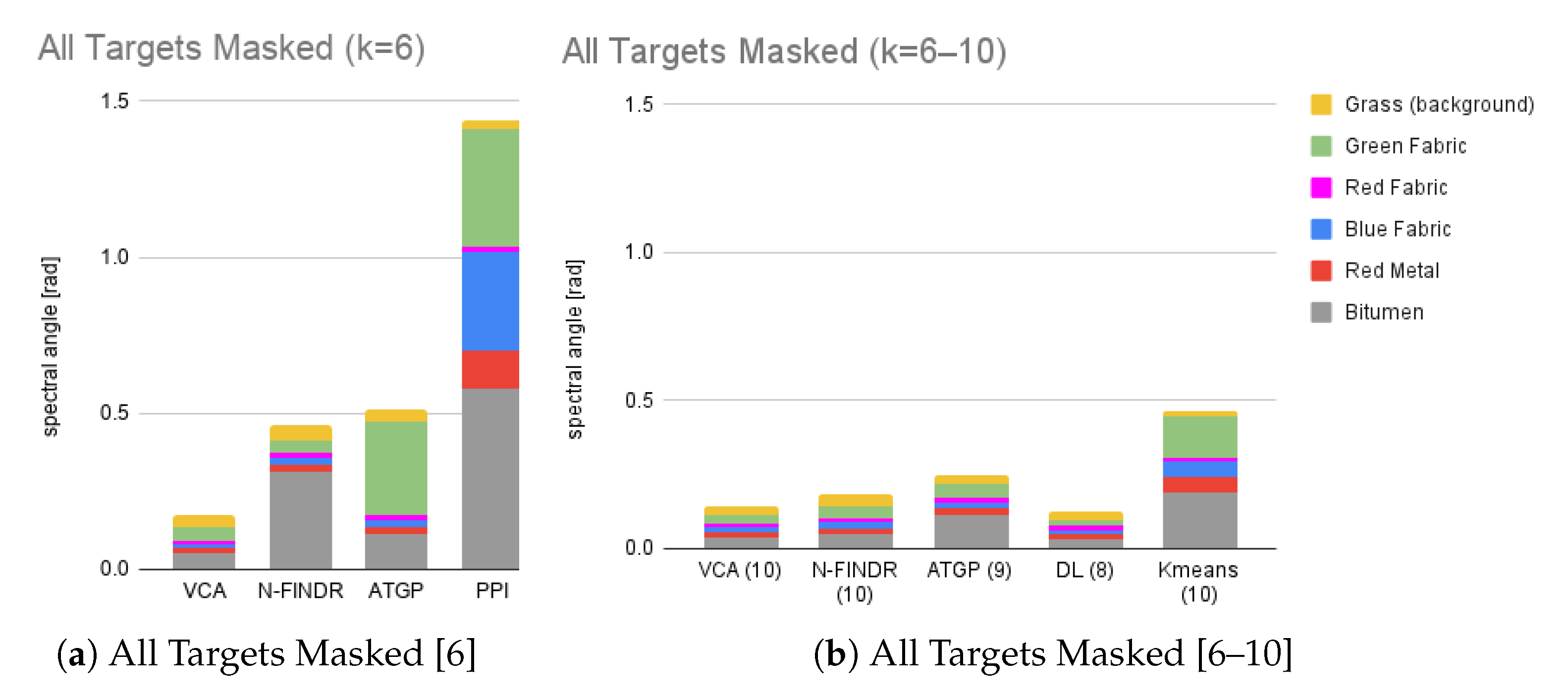
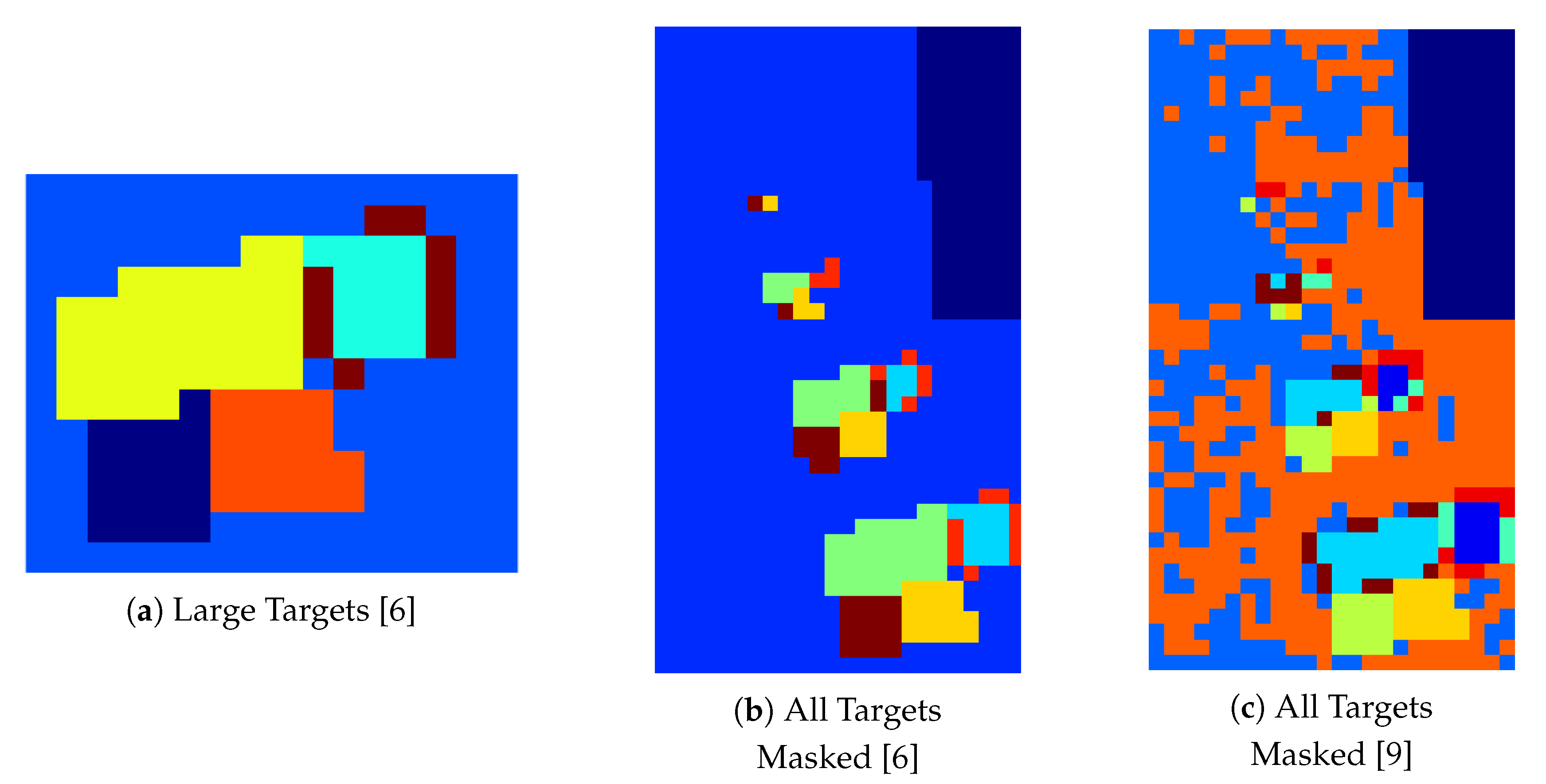
- All Targets Masked (42 × 24, with a total of 884 valid pixels) is the same as above, but with non-homogeneous areas in the background masked out. The expected value of K is 6.
- Small Targets (12 × 12) contains only the 0.25 and 0.5m targets. As the HySpex data are resampled to a m grid, in this subset all pixels are mixed with the exception of the surrounding grass. This allows testing endmember extraction algorithms without the pure pixel assumption. The value K does not apply here due to the high mixing degree of the pixels.
- Large Targets (13 × 16) represents the subset containing only the m targets (five in total) and the surrounding homogeneous grass. This subset is aimed at providing the easiest setting for dimensionality estimation, endmember extraction with pure pixel assumption, and abundance estimation. The expected value of K is 6. In Figure 4d the locations of the representative image elements used for the creation of the spectral library used in this paper are marked in white.
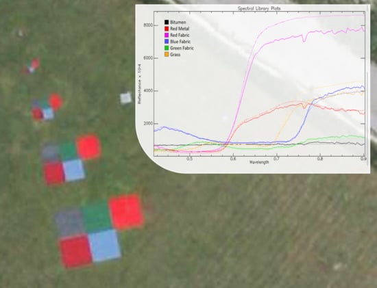
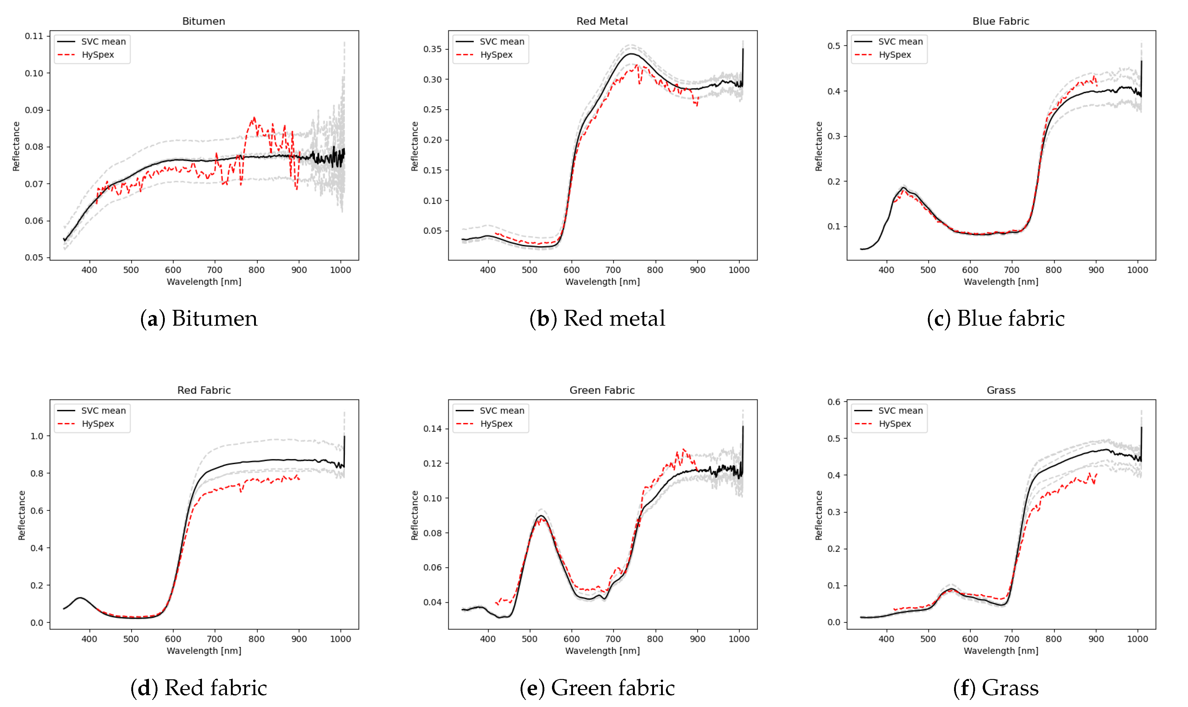
2.3. Field Measurements
3. Dimensionality Estimation
4. Endmember Extraction
4.1. Clustering Experiment
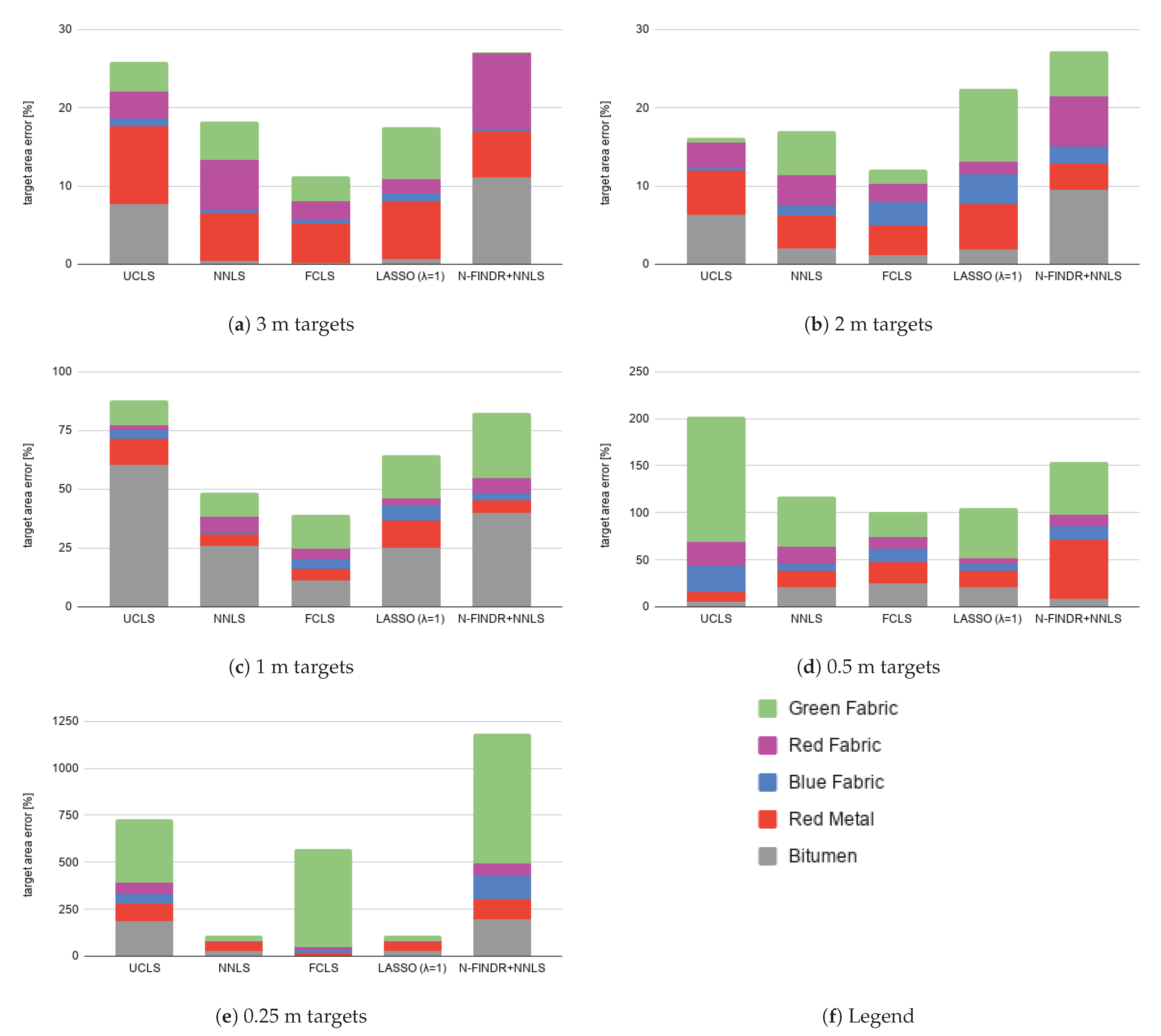
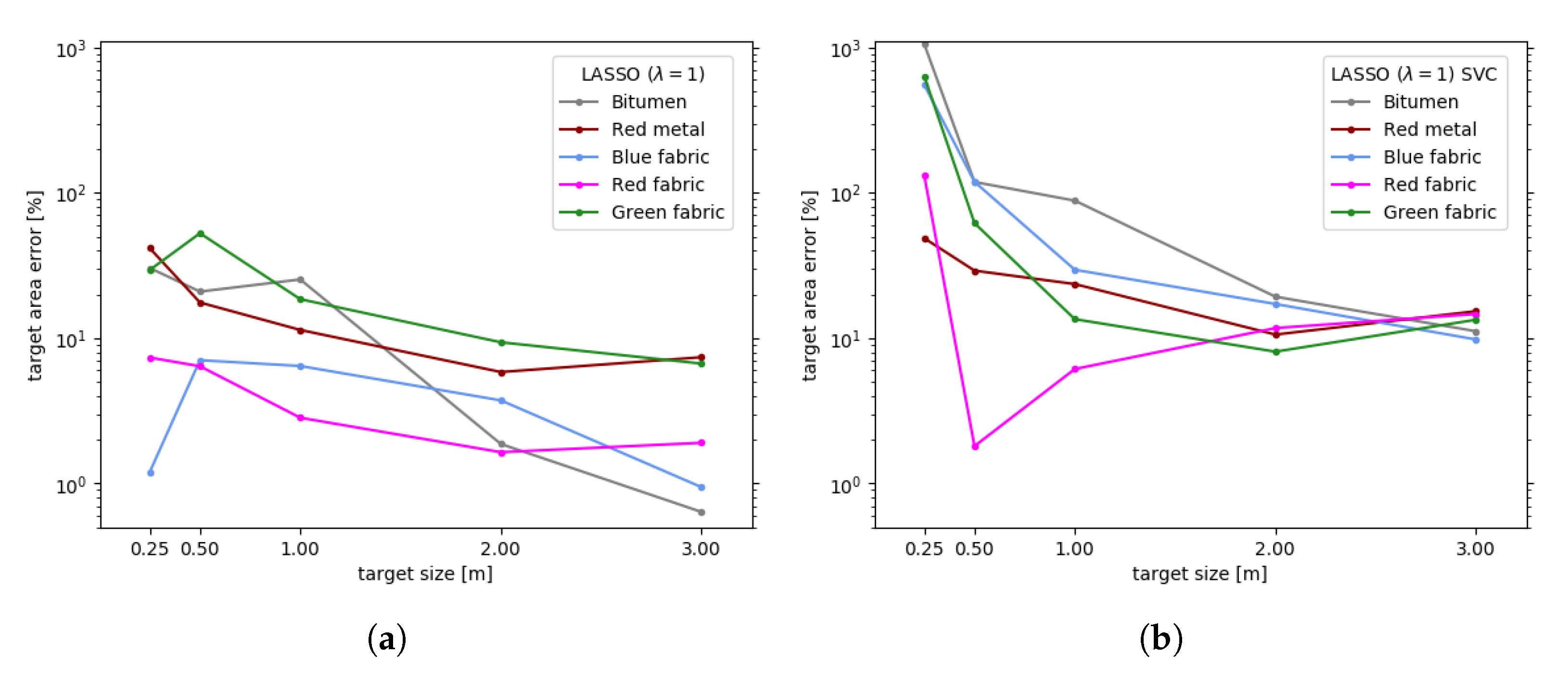
5. Abundance Estimation
6. Other Applications
6.1. Joint Endmember Extraction and Abundance Estimation
6.2. Hidden Target Detection
7. Conclusions
- The confirmation of overestimation by the most used dimensionality estimation method for imaging spectrometer data, HySime, in non-ideal settings, i.e., when applied to images too small in size with non-zero noise contribution.
- The comparison between algorithms working with or without the pure pixel assumption assessed on real data for different targets, suggesting that the latter family of algorithms may perform slightly better at handling complex, highly mixed data. To the best of our knowledge, this is the first time that a comparison between algorithms working with or without the pure pixel assumption is made on real data. In the past, such assessment was made on synthetic images [1].
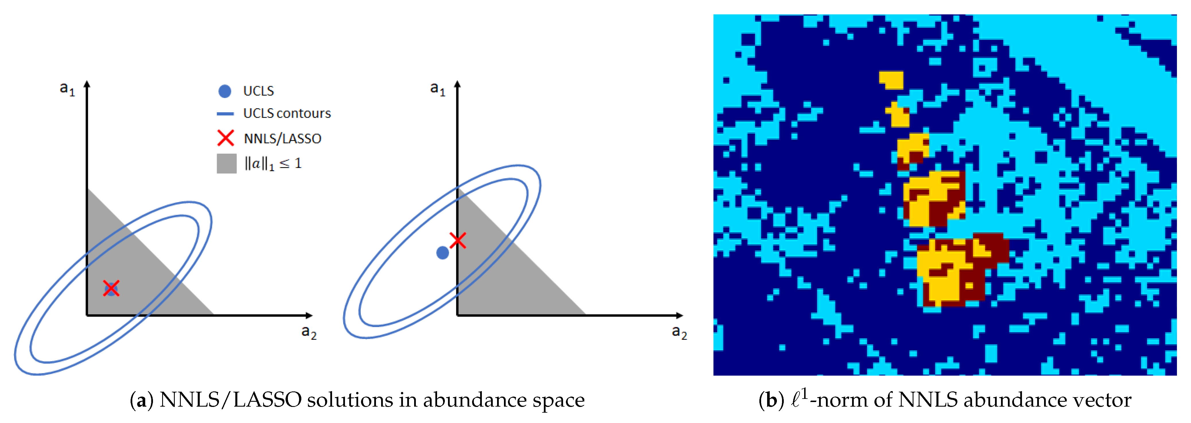
- The equivalence between the NNLS and the LASSO methods for specific cases.
- The effects of enforcing the sum-to-one constraint in FCLS, often used in abundance estimation in the literature, which may introduce severe distortions in the case of image elements with a high degree of mixture. The last aspect adds up to the distortions introduced by FCLS whenever an incomplete spectral library is used [2].
Author Contributions
Funding
Data Availability Statement
Acknowledgments
Conflicts of Interest
Abbreviations
| ATGP | Automatic Target Generation Process |
| DESIS | DLR Earth Sensing Imaging Spectrometer |
| DL | Dictionary Learning |
| DLR | German Aerospace Center |
| DLR HySU | DLR HyperSpectral Unmixing |
| FCLS | Fully Constrained Least Squares |
| GSD | Ground Sampling Distance |
| GPS | Global Positioning System |
| HFC | Harsanyi–Farrand–Chang |
| HySime | Hyperspectral Signal Identification by Minimum Error |
| IMU | Inertial Measurement Unit |
| LASSO | Least Absolute Shrinkage and Selection Operator |
| MNF | Minimum Noise Fraction |
| NMF | Non-negative Matrix Factorization |
| NNLS | Non-negative Least Squares |
| OSP | Orthogonal Subspace Projection |
| PCA | Principal Components Analysis |
| PPI | Pixel Purity Index |
| PSF | Point Spread Function |
| SISAL | Simplex Identification via Split Augmented Lagrangian |
| SNR | Signal-to-Noise Ratio |
| SU | Spectral Unmixing |
| SVC | Spectra Vista Corporation |
| SWIR | Shortwave Infrared |
| UCLS | Unconstrained Least Squares |
| VCA | Vertex Component Analysis |
| VNIR | Visible and Near Infrared |
Appendix A. Target Additional Information

| Target Area [m] | 3 m | 2 m | 1 m | 0.5 m | 0.25 m |
|---|---|---|---|---|---|
| Bitumen | 9.030 | 4.000 | 0.985 | 0.258 | 0.062 |
| Red metal | 8.850 | 3.990 | 0.910 | 0.250 | 0.060 |
| Blue fabric | 8.940 | 4.060 | 1.005 | 0.250 | 0.061 |
| Red fabric | 9.211 | 3.990 | 1.000 | 0.253 | 0.065 |
| Green fabric | 9.075 | 4.020 | 1.000 | 0.248 | 0.066 |
| Target Area [pix] | 3 m | 2 m | 1 m | 0.5 m | 0.25 m |
|---|---|---|---|---|---|
| Bitumen | 18.429 | 8.163 | 2.010 | 0.526 | 0.128 |
| Red metal | 18.061 | 8.143 | 1.857 | 0.510 | 0.123 |
| Blue fabric | 18.245 | 8.286 | 2.051 | 0.510 | 0.125 |
| Red fabric | 18.798 | 8.143 | 2.041 | 0.515 | 0.133 |
| Green fabric | 18.521 | 8.204 | 2.041 | 0.505 | 0.135 |
References
- Bioucas-Dias, J.M.; Plaza, A.; Dobigeon, N.; Parente, M.; Du, Q.; Gader, P.; Chanussot, J. Hyperspectral Unmixing Overview: Geometrical, Statistical, and Sparse Regression-Based Approaches. IEEE J. Sel. Top. Appl. Earth Obs. Remote Sens. 2012, 5, 354–379. [Google Scholar] [CrossRef] [Green Version]
- Cerra, D.; Müller, R.; Reinartz, P. Noise Reduction in Hyperspectral Images Through Spectral Unmixing. IEEE Geosci. Remote Sens. Lett. 2014, 11, 109–113. [Google Scholar] [CrossRef] [Green Version]
- Altmann, Y.; Halimi, A.; Dobigeon, N.; Tourneret, J.Y. Supervised nonlinear spectral unmixing using a post-nonlinear mixing model for hyperspectral imagery. IEEE Trans. Geosci. Remote Sens. 2012, 21, 3017–3025. [Google Scholar]
- Keshava, N.; Mustard, J.F. Spectral unmixing. IEEE Signal Process. Mag. 2002, 19, 44–57. [Google Scholar] [CrossRef]
- Zhu, F. Hyperspectral unmixing: Ground truth labeling, datasets, benchmark performances and survey. arXiv 2017, arXiv:1708.05125. [Google Scholar]
- Imbiriba, T.; Borsoi, R.; Bermudez, J. Low-Rank Tensor Modeling for Hyperspectral Unmixing Accounting for Spectral Variability. IEEE Trans. Geosci. Remote Sens. 2019, 58, 1833–1842. [Google Scholar] [CrossRef] [Green Version]
- HySU Download Link. Available online: https://www.dlr.de/eoc/en/desktopdefault.aspx/tabid-12760/22294_read-73262/ (accessed on 7 June 2021).
- Heylen, R.; Parente, M.; Gader, P. A Review of Nonlinear Hyperspectral Unmixing Methods. IEEE J. Sel. Top. Appl. Earth Obs. Remote Sens. 2014, 7, 1844–1868. [Google Scholar] [CrossRef]
- Zhang, G.; Cerra, D.; Müller, R. Shadow Detection and Restoration for Hyperspectral Images Based on Nonlinear Spectral Unmixing. Remote Sens. 2020, 12, 3985. [Google Scholar] [CrossRef]
- Dobigeon, N.; Altmann, Y.; Brun, N.; Moussaoui, S. Linear and Nonlinear Unmixing in Hyperspectral Imaging. In Resolving Spectral Mixtures with Applications from Ultrafast Time-Resolved Spectroscopy to Super-Resolution Imaging; Ruckebusch, C., Ed.; Data Handling in Science and Technology; Elsevier: Amsterdam, The Netherlands, 2016; Volume 30, pp. 185–224. [Google Scholar] [CrossRef]
- Institute, D.R.S.T. Airborne Imaging Spectrometer HySpex. JLSRF 2016, 2, A93. [Google Scholar] [CrossRef] [Green Version]
- Kurz, F.; Türmer, S.; Meynberg, O.; Rosenbaum, D.; Runge, H.; Reinartz, P.; Leitloff, J. Low-cost Systems for real-time Mapping Applications. Photogramm. Fernerkund. Geoinf. 2012, 159–176. [Google Scholar] [CrossRef]
- Holben, B.; Eck, T.; Slutsker, I.; Tanré, D.; Buis, J.; Setzer, A.; Vermote, E.; Reagan, J.; Kaufman, Y.; Nakajima, T.; et al. AERONET—A Federated Instrument Network and Data Archive for Aerosol Characterization. Remote Sens. Environ. 1998, 66, 1–16. [Google Scholar] [CrossRef]
- Krauß, T.; d’Angelo, P.; Schneider, M.; Gstaiger, V. The Fully Automatic Optical Processing System CATENA at DLR. ISPRS Int. Arch. Photogramm. Remote Sens. Spat. Inf. Sci. 2013, XL-1/W, 177–181. [Google Scholar] [CrossRef] [Green Version]
- Baumgartner, A.; Köhler, C.H. Transformation of point spread functions on an individual pixel scale. Opt. Express 2020, 28, 38682–38697. [Google Scholar] [CrossRef] [PubMed]
- Schwind, P.; Schneider, M.; Müller, R. Improving HySpex Sensor Co-Registration Accuracy using BRISK and Sensor-model based RANSAC. ISPRS Arch. 2014, XL-1, 371–376. [Google Scholar] [CrossRef] [Green Version]
- Müller, R.; Lehner, M.; Müller, R.; Reinartz, P.; Schroeder, M.; Vollmer, B. A program for direct georeferencing of airborne and spaceborne line scanner images. Int. Arch. Photogramm. Remote Sens. Spat. Inf. Sci. 2002, 34, 148–153. [Google Scholar]
- Richter, R.; Schläpfer, D. Geo-atmospheric processing of airborne imaging spectrometry data. Part 2: Atmospheric/topographic correction. Int. J. Remote Sens. 2002, 23, 2631–2649. [Google Scholar] [CrossRef]
- Richter, R. Correction of satellite imagery over mountainous terrain. Appl. Opt. 1998, 37, 4004–4015. [Google Scholar] [CrossRef]
- Bioucas-Dias, J.; Nascimento, J. Hyperspectral subspace identification. IEEE Trans. Geosci. Remote Sens. 2008, 46, 2435–2445. [Google Scholar] [CrossRef] [Green Version]
- Wang, C.M.; Chen, C.; Chung, Y.N.; Yang, S.C.; Chung, P.C.; Yang, C.W.; Chang, C.I. Detection of spectral signatures in multispectral MR images for classification. IEEE Trans. Med. Imaging 2003, 22, 50–61. [Google Scholar] [CrossRef]
- Bioucas Dias, J.M. Code, University of Lisbon. Available online: http://www.lx.it.pt/~bioucas/code.htm (accessed on 21 June 2021).
- Gerg, I. Hyperspectral Toolbox. Available online: https://github.com/isaacgerg/matlabHyperspectralToolbox (accessed on 21 June 2021).
- Chang, C. A Review of Virtual Dimensionality for Hyperspectral Imagery. IEEE J. Sel. Top. Appl. Earth Obs. Remote Sens. 2018, 11, 1285–1305. [Google Scholar] [CrossRef]
- Prades, J.; Safont, G.; Salazar, A.; Vergara, L. Estimation of the Number of Endmembers in Hyperspectral Images Using Agglomerative Clustering. Remote Sens. 2020, 12, 3585. [Google Scholar] [CrossRef]
- Drumetz, L.; Veganzones, M.A.; Marrero Gómez, R.; Tochon, G.; Mura, M.D.; Licciardi, G.A.; Jutten, C.; Chanussot, J. Hyperspectral Local Intrinsic Dimensionality. IEEE Trans. Geosci. Remote Sens. 2016, 54, 4063–4078. [Google Scholar] [CrossRef] [Green Version]
- Ghamisi, P.; Yokoya, N.; Li, J.; Liao, W.; Liu, S.; Plaza, J.; Rasti, B.; Plaza, A. Advances in Hyperspectral Image and Signal Processing: A Comprehensive Overview of the State of the Art. IEEE Geosci. Remote Sens. Mag. 2017, 5, 37–78. [Google Scholar] [CrossRef] [Green Version]
- Berman, M.; Hao, Z.; Stone, G.; Guo, Y. An Investigation Into the Impact of Band Error Variance Estimation on Intrinsic Dimension Estimation in Hyperspectral Images. IEEE J. Sel. Top. Appl. Earth Obs. Remote Sens. 2018, 11, 3279–3296. [Google Scholar] [CrossRef]
- Plaza, J.; Hendrix, E.; García Fernandez, I.; Martín, G.; Plaza, A. On Endmember Identification in Hyperspectral Images Without Pure Pixels: A Comparison of Algorithms. J. Math. Imaging Vis. 2012, 42, 163–175. [Google Scholar] [CrossRef]
- Alonso, K.; Bachmann, M.; Burch, K.; Carmona, E.; Cerra, D.; de los Reyes, R.; Dietrich, D.; Heiden, U.; Hölderlin, A.; Ickes, J.; et al. Data Products, Quality and Validation of the DLR Earth Sensing Imaging Spectrometer (DESIS). Sensors 2019, 19, 4471. [Google Scholar] [CrossRef] [Green Version]
- Nascimento, J.M.P.; Dias, J.M.B. Vertex component analysis: A fast algorithm to unmix hyperspectral data. IEEE Trans. Geosci. Remote Sens. 2005, 43, 898–910. [Google Scholar] [CrossRef] [Green Version]
- Winter, M.E. N-FINDR: An Algorithm for Fast Autonomous Spectral End-Member Determination in Hyperspectral Data. In Imaging Spectrometry V; Descour, M.R., Shen, S.S., Eds.; International Society for Optics and Photonics, SPIE: Washington, DC, USA, 1999; pp. 266–275. [Google Scholar] [CrossRef]
- Ren, H.; Chang, C. Automatic spectral target recognition in hyperspectral imagery. IEEE Trans. Aerosp. Electron. Syst. 2003, 39, 1232–1249. [Google Scholar]
- Chang, C.; Chen, S.; Li, H.; Chen, H.; Wen, C. Comparative Study and Analysis Among ATGP, VCA, and SGA for Finding Endmembers in Hyperspectral Imagery. IEEE J. Sel. Top. Appl. Earth Obs. Remote Sens. 2016, 9, 4280–4306. [Google Scholar] [CrossRef]
- Therien, C. PySptools. Available online: https://pysptools.sourceforge.io/index.html (accessed on 21 June 2021).
- Boardman, J.W. Geometric mixture analysis of imaging spectrometry data. In Proceedings of the IGARSS ’94-1994 IEEE International Geoscience and Remote Sensing Symposium, Pasadena, CA, USA, 8–12 August 1994; Volume 4, pp. 2369–2371. [Google Scholar] [CrossRef]
- Bioucas-Dias, J.M. A variable splitting augmented Lagrangian approach to linear spectral unmixing. In Proceedings of the 2009 First Workshop on Hyperspectral Image and Signal Processing: Evolution in Remote Sensing, Grenoble, France, 26–28 August 2009. [Google Scholar] [CrossRef] [Green Version]
- Miao, L.; Qi, H. Endmember Extraction From Highly Mixed Data Using Minimum Volume Constrained Nonnegative Matrix Factorization. IEEE Trans. Geosci. Remote Sens. 2007, 45, 765–777. [Google Scholar] [CrossRef]
- Pedregosa, F.; Varoquaux, G.; Gramfort, A.; Michel, V.; Thirion, B.; Grisel, O.; Blondel, M.; Prettenhofer, P.; Weiss, R.; Dubourg, V.; et al. Scikit-learn: Machine Learning in Python. J. Mach. Learn. Res. 2011, 12, 2825–2830. [Google Scholar]
- ITAKURA, F. Analysis synthesis telephony based on the maximum likelihood method. In Proceedings of the 6th International Congress on Acoustics, Tokyo, Japan, 21–28 August 1968. [Google Scholar]
- MacQueen, J. Some methods for classification and analysis of multivariate observations. In Proceedings of the Fifth Berkeley Symposium on Mathematical Statistics and Probability, Oakland, CA, USA, 27 December 1965–7 January 1966; pp. 281–297. [Google Scholar]
- Kruse, F.A.; Lefkoff, A.; Boardman, J.; Heidebrecht, K.; Shapiro, A.; Barloon, P.; Goetz, A. The spectral image processing system (SIPS)-interactive visualization and analysis of imaging spectrometer data. In AIP Conference Proceedings; American Institute of Physics: Pasadena, CA, USA, 1993; pp. 192–201. [Google Scholar]
- Shah, D.; Zaveri, T.; Dixit, R. Hyperspectral Endmember Extraction Algorithm Using Convex Geometry and K-Means. In Emerging Technology Trends in Electronics, Communication and Networking; Gupta, S., Sarvaiya, J.N., Eds.; Springer: Singapore, 2020; pp. 189–200. [Google Scholar]
- Martin, G.; Plaza, A. Region-Based Spatial Preprocessing for Endmember Extraction and Spectral Unmixing. IEEE Geosci. Remote Sens. Lett. 2011, 8, 745–749. [Google Scholar] [CrossRef] [Green Version]
- Iordache, M.D.; Bioucas-Dias, J.; Plaza, A. Sparse Unmixing of Hyperspectral Data. IEEE Trans. Geosci. Remote Sens. 2011, 49, 2014–2039. [Google Scholar] [CrossRef] [Green Version]
- Tibshirani, R. Regression Shrinkage and Selection via the Lasso. J. R. Stat. Society. Ser. B 1996, 58, 267–288. [Google Scholar] [CrossRef]
- SPAMS (SPArse Modeling Software). Available online: http://spams-devel.gforge.inria.fr/index.html (accessed on 21 June 2021).
- Mairal, J.; Bach, F.R.; Ponce, J.; Sapiro, G. Online Learning for Matrix Factorization and Sparse Coding. J. Mach. Learn. Res. 2010, 11, 19–60. [Google Scholar]
- Mairal, J.; Bach, F.; Ponce, J.; Sapiro, G. Online Dictionary Learning for Sparse Coding. In Proceedings of the International Conference on Machine Learning, Montreal, QC, Canada, 14–18 June 2009. [Google Scholar]


| Dataset | Full | All Targets | All Targets Masked | Large Targets |
|---|---|---|---|---|
| Nr. of Pixels | 10,578 | 1008 | 884 | 208 |
| K | 12+ | 7–9 | 6 | 6 |
| HySime | 16 | 18 | 20 | 46 |
| HFC () | 57 | 7 | 7 | 6 |
| HFC () | 48 | 7 | 7 | 6 |
| HFC () | 40 | 7 | 7 | 5 |
| Material | 3m | 2m | 1m | 0.5m | 0.25m | |||||
|---|---|---|---|---|---|---|---|---|---|---|
| UCLS | ||||||||||
| Bitumen | 19.839 | (+7.7%) | 8.678 | (+6.3) | 3.221 | (+60%) | 0.555 | (+5.5%) | 0.363 | (+185%) |
| Red metal | 16.255 | (−10%) | 7.682 | (−5.7%) | 1.649 | (−11%) | 0.457 | (−10%) | 0.009 | (>−93%) |
| Blue fabric | 18.072 | (−0.9%) | 8.250 | (−0.4%) | 1.974 | (−3.8%) | 0.372 | (−27%) | 0.057 | (>) |
| Red fabric | 18.142 | (−3.5%) | 7.886 | (−3.2%) | 2.001 | (−1.9%) | 0.380 | ( −26%) | 0.051 | (−62%) |
| Green fabric | 17.824 | (−3.8%) | 8.156 | (−0.6%) | 1.823 | (−11%) | −0.164 | (−133%) | −0.319 | (#x2212;336%) |
| Average | 5.2% | 3.2% | 18% | >40% | >146% | |||||
| NNLS | ||||||||||
| Bitumen | 18.356 | (−0.4%) | 8.000 | (−2.0%) | 2.534 | (+26%) | 0.416 | (−21%) | 0.166 | (+30%) |
| Red metal | 16.943 | (−6.2%) | 7.800 | (−4.2%) | 1.767 | (−4.8%) | 0.600 | (+18%) | 0.072 | (−42%) |
| Blue fabric | 18.175 | (−0.4%) | 8.401 | (+1.4%) | 2.065 | (+0.7%) | 0.474 | (−7.0%) | 0.124 | (−1.2%) |
| Red fabric | 17.603 | (−6.4%) | 7.833 | (−3.8%) | 1.907 | (−6.6%) | 0.418 | (−19%) | 0.142 | (+7.3%) |
| Green fabric | 17.616 | (−4.9%) | 7.739 | (−5.7%) | 1.832 | (−10%) | 0.239 | (−53%) | 0.175 | (+29%) |
| Average | 3.6% | 3.4% | 9.7% | 23% | 22% | |||||
| FCLS | ||||||||||
| Bitumen | 18.465 | (+0.2%) | 8.072 | (−1.1%) | 2.233 | (+11%) | 0.395 | (−25%) | 0.123 | (−3.6%) |
| Red metal | 17.157 | (−5.0%) | 7.825 | (−3.9%) | 1.766 | (−4.9%) | 0.627 | (+23%) | 0.141 | (+15%) |
| Blue fabric | 18.328 | (+0.5%) | 8.525 | (+2.9%) | 2.138 | (+4.2%) | 0.439 | (−14%) | 0.106 | (−15%) |
| Red fabric | 18.361 | (−2.3%) | 7.955 | (−2.3%) | 1.951 | (−4.4%) | 0.449 | (−13%) | 0.110 | (−17%) |
| Green fabric | 17.909 | (−3.3%) | 8.053 | (−1.8%) | 2.340 | (+15%) | 0.638 | (+26%) | 0.838 | (+520%) |
| Average | 2.3% | 2.4% | 7.9% | 20% | >114% | |||||
| LASSO (λ = 1) | ||||||||||
| Bitumen | 18.311 | (−0.6%) | 8.011 | (−) | 2.519 | (+25%) | 0.416 | (−21%) | 0.166 | (+30%) |
| Red metal | 16.727 | (−7.4%) | 7.667 | (−5.8%) | 1.646 | (−11%) | 0.600 | (+18%) | 0.072 | (−42%) |
| Blue fabric | 18.417 | (+0.9%) | 8.595 | (+3.7%) | 2.183 | (+6.4%) | 0.474 | (−7.0%) | 0.124 | (−1.2%) |
| Red fabric | 18.440 | (−1.9%) | 8.009 | (−1.6%) | 1.983 | (−2.8%) | 0.482 | (−6.4%) | 0.142 | (+7.3%) |
| Green fabric | 17.283 | (−6.7%) | 7.436 | (−9.4%) | 1.663 | (−19%) | 0.239 | (−53%) | 0.175 | (+29%) |
| Average | 3.5% | 4.5% | 13% | 21% | 22% | |||||
| N-FINDR+NNLS | ||||||||||
| Bitumen | 16.383 | (−11%) | 7.391 | (−9.5%) | 2.809 | (+40%) | 0.571 | (+8.6%) | 0.378 | (+196%) |
| Red metal | 16.990 | (−5.9%) | 7.869 | (−3.4%) | 1.956 | (+5.3%) | 0.828 | (+62%) | 0.258 | (+111%) |
| Blue fabric | 18.211 | (−0.2%>) | 8.474 | (+2.3%) | 2.114 | (+3.1%) | 0.585 | (+15%) | 0.278 | (+122%) |
| Red fabric | 16.967 | (−9.7%) | 7.629 | (−6.3%) | 1.910 | (−6.4%) | 0.453 | (−12%) | 0.216 | (+63%) |
| Green fabric | 18.545 | (+0.1%) | 8.682 | (+5.8%) | 2.611 | (+28%) | 0.789 | (+56%) | 1.073 | (+693%) |
| Average | 5.4% | 5.4% | 16% | 31% | 237% | |||||
Publisher’s Note: MDPI stays neutral with regard to jurisdictional claims in published maps and institutional affiliations. |
© 2021 by the authors. Licensee MDPI, Basel, Switzerland. This article is an open access article distributed under the terms and conditions of the Creative Commons Attribution (CC BY) license (https://creativecommons.org/licenses/by/4.0/).
Share and Cite
Cerra, D.; Pato, M.; Alonso, K.; Köhler, C.; Schneider, M.; de los Reyes, R.; Carmona, E.; Richter, R.; Kurz, F.; Reinartz, P.; et al. DLR HySU—A Benchmark Dataset for Spectral Unmixing. Remote Sens. 2021, 13, 2559. https://doi.org/10.3390/rs13132559
Cerra D, Pato M, Alonso K, Köhler C, Schneider M, de los Reyes R, Carmona E, Richter R, Kurz F, Reinartz P, et al. DLR HySU—A Benchmark Dataset for Spectral Unmixing. Remote Sensing. 2021; 13(13):2559. https://doi.org/10.3390/rs13132559
Chicago/Turabian StyleCerra, Daniele, Miguel Pato, Kevin Alonso, Claas Köhler, Mathias Schneider, Raquel de los Reyes, Emiliano Carmona, Rudolf Richter, Franz Kurz, Peter Reinartz, and et al. 2021. "DLR HySU—A Benchmark Dataset for Spectral Unmixing" Remote Sensing 13, no. 13: 2559. https://doi.org/10.3390/rs13132559
APA StyleCerra, D., Pato, M., Alonso, K., Köhler, C., Schneider, M., de los Reyes, R., Carmona, E., Richter, R., Kurz, F., Reinartz, P., & Müller, R. (2021). DLR HySU—A Benchmark Dataset for Spectral Unmixing. Remote Sensing, 13(13), 2559. https://doi.org/10.3390/rs13132559