Abstract
Remote sensing images have been widely applied in various industries; nevertheless, the resolution of such images is relatively low. Panchromatic sharpening (pan-sharpening) is a research focus in the image fusion domain of remote sensing. Pan-sharpening is used to generate high-resolution multispectral (HRMS) images making full use of low-resolution multispectral (LRMS) images and panchromatic (PAN) images. Traditional pan-sharpening has the problems of spectral distortion, ringing effect, and low resolution. The convolutional neural network (CNN) is gradually applied to pan-sharpening. Aiming at the aforementioned problems, we propose a distributed fusion framework based on residual CNN (RCNN), namely, RDFNet, which realizes the data fusion of three channels. It can make the most of the spectral information and spatial information of LRMS and PAN images. The proposed fusion network employs a distributed fusion architecture to make the best of the fusion outcome of the previous step in the fusion channel, so that the subsequent fusion acquires much more spectral and spatial information. Moreover, two feature extraction channels are used to extract the features of MS and PAN images respectively, using the residual module, and features of different scales are used for the fusion channel. In this way, spectral distortion and spatial information loss are reduced. Employing data from four different satellites to compare the proposed RDFNet, the results of the experiment show that the proposed RDFNet has superior performance in improving spatial resolution and preserving spectral information, and has good robustness and generalization in improving the fusion quality.
1. Introduction
For a long time, remote sensing images have been widely applied in various industries, such as agricultural yield prediction, plant diseases and pests detection, disaster prediction, geological exploration, national defense, vegetation coverage and land use, environmental change detection, and so on [1,2]. However, due to the limitations of satellite sensor technology, it is impossible to obtain images with high spatial resolution and high spectral resolution at the same time. Only PAN images with high spatial resolution and low spectral resolution and MS images with low spatial resolution and high spectral resolution can be obtained [3]. Notwithstanding, a variety of fields need to make use of images with both high spatial resolution and high spectral resolution (HRHM), and even images with high temporal resolution.
HRHM images are obtained by taking advantage of the redundant and complementary information of high spatial resolution and low spectral resolution images and high spectral resolution and low spatial resolution (LRMS) images. At present, the major image processing technologies consist of image enhancement, super-resolution reconstruction, image fusion, and so on. One of the most used and main technologies is image fusion, which generates a higher quality and more abundant information image by making good use of multiple images of the same object in different shapes. Certain fusion methods can be helpful for improving our visual perception and making more accurate decisions.
Fusion technology of multispectral (MS) images and panchromatic (PAN) images (pan-sharpening) [4] is one of the critical researches in the field of remote sensing image processing. The MS and PAN images are processed by fusion technology, which can make full use of spatial details and spectral information to improve spatial resolution and spectral resolution. The processed image can be used for remote sensing image classification, target recognition, environmental change detection, disaster prediction and monitoring, geological exploration, national defense, vegetation coverage and land use, urban construction, and other aspects [1,5]. In this way, we can achieve more reliable and richer information, clearer spatial details, and more recognizable images so as to facilitate decision makers to make more accurate decisions.
Pan-sharpening methods can be roughly divided into traditional methods and deep-learning-based methods. The traditional methods include the component substitution (CS) method, multiresolution analysis (MRA) method, hybrid method, and model-based method [4]. The CS-based method converts a MS image from one projection space to another projection space, separates the spatial structure from the MS image, and then replaces the separated spatial information components with a high spatial resolution image to generate a new image [4]. Then, the generated image is transformed inversely and the HRMS image can be obtained—for instance, intensity–hue–saturation (IHS) [6], generalized IHS [7], fast IHS [8], adaptive IHS [9], and other variants. The above methods are simple and fast. However, there are the problems of spectral distortion, and fusion quality is relatively low; further, this method is inefficient for large amounts of remote sensing data. Principal component analysis (PCA) is a statistical analysis method that converts relevant data into irrelevant or relatively low correlation data, then replaces the original first principal component image with a PAN image [10,11,12]. PCA can transform the problem from high-dimensional space to low-dimensional space, and can use any number of bands, but it is prone to spectral distortion. Brovey transform (BT) [7] is used to normalize the three bands and then multiply the result by the corresponding weight data to obtain the fused image. Gram–Schmidt (GS) [1] pan-sharpening is an extension of the PCA method. It avoids the spectral response range inconsistency caused by the overconcentration of some band information and the new high spatial resolution panchromatic band wavelength range expansion. It can maintain the consistency of spectral information before and after fusion. PCA, BT, and GS are widely used and even integrated in software. Nevertheless, spectral distortion and oversharpening still exist. The MRA method [13] is also known as the multiscale analysis method. For example, wavelet transform (WT) [14,15] has no translation invariance; it cannot best represent the edge of the image, and it cannot effectively extract the geometric features of the image. In addition, the sampling method leads to spectrum aliasing, which results in a ringing phenomenon. Due to the problems of WT, a fusion algorithm based on contourlet transform (CT) [16,17] was proposed. CT effectively utilizes the better performance of contourlet in processing two-dimensional and higher-dimensional images. It also has the characteristics of multidirection and anisotropy. There is still no translation invariance. Non-subsampled contourlet transform (NSCT) [18] can not only decompose the image in multiscale and multidirection, but also has translation invariance. Smoothing-filter-based intensity modulation (SFIM) [19] is used to match a high-resolution PAN image to LRMS images by smoothing filter. This method is similar to WT, but it is simpler than WT. The proposed method in [20] combined the advantages of CS and MRA, reducing spectral distortion and improving the spatial resolution. Sparse representation (SR) can process data efficiently, and combine with WT for remote sensing image fusion. On this basis, different training dictionaries and fusion rules have been proposed to improve the algorithm, and good fusion results were achieved [21,22,23]. Other decomposition methods in the transform domain include Laplace pyramid decomposition [24,25], curvelet transform [26,27], and so on. In the model-based fusion method, the hierarchical Bayesian model is used to fuse multiple band images with different spectral resolutions and spatial resolutions [28]. The online coupled dictionary learning method (OCDL) makes full use of the spatial information of PAN image to reduce spectral distortion [29]. Sparse matrix decomposition [30] learns a spectral dictionary from LRMS images and then predicts HRHM images based on the learned spectral dictionary and high spatial resolution images. Although the spectral distortion is reduced, the spatial information of the high spatial resolution image cannot be fully utilized, which results in the spatial resolution of the fused image being inferior to that of reference image. In addition, in order to make full use of the high-frequency information of PAN and intensity images, the low-rank decomposition method is used to decompose the high-frequency information into low-rank component and sparse component [31]. Then, the low-rank component and sparse component are fused by appropriate fusion rules, and the fused image is obtained by merging and inverse transformation. Although traditional methods are improving, spectral distortion and loss of spatial details are common problems.
With the development of deep learning (DL) technology, more and more scholars use DL for remote sensing image fusion. CNN is used most in fusion and its model is improved. The super-resolution convolution neural network (SRCNN) [32,33,34] uses a full convolution network to build a nonlinear model of low-resolution image mapping to generate a high-resolution image. SRCNN is relatively shallow, with only three layers, which is relatively easy to implement. However, SRCNN can only be used for a single image. Based on SRCNN, pan-sharpening by convolutional neural network (PNN) [35,36,37] has been proposed, which directly uses a relatively simple three-layer convolution to pan-sharpen making the best of nonlinearity. Yet, SRCNN and PNN may bring about overfitting. Then, residual learning [38] was introduced into the deep convolution neural network—that is, residual network based panchromatic sharpening (DRPNN) [39]. DRPNN makes the most of the nonlinearity of the network to improve spatial resolution and retain spectral information. The RCNN uses the difference between the HRMS image and the LRMS image to pan-sharpen. In order to preserve spatial and spectral information, PanNet was proposed in [40], which adds upsampled MS to the output and trains PanNet parameters in high-pass filtering domain. PanNet is robust to various satellites. MSDCNN was proposed in [41], and consists of two branches to extract features. One is fundamental three-layer CNN, the other is a deeper multiscale feature extraction, which employs skip connection. The application of multiscale features is more conducive to preserving spectral and spatial information, and skip connection is more conducive to the convergence of the network. However, MSDCNN extracts the features of MS and PAN images simultaneously. 3D-CNN [42] fuses MS images and hyperspectral (HS) images to generate high-resolution hyperspectral (HRHS) images. The idea of 3D-CNN is similar to that of 2D-CNN. In order to reduce the amount of computation, it is necessary to use PCA for dimensionality reduction of HS images. The literature in [43] proposes a two-branch feature extraction network, namely, RSIFNN. RSIFNN extracts features from MS and PAN images, respectively, then fuses the features. In order to preserve much more spectral information, RSIFNN introduces residual learning in the last layer. A-PNN was proposed in [44]; A-PNN can not only perform registered images fusion but also carry out unregistered images and multisensor data fusion. A two-stream fusion network (TFNet) was proposed in [45] and comprised three parts. The first extracts features from MS and PAN images, respectively. The second concatenates MS and PAN features, then represents spectral and spatial information, simultaneously. Finally, the pan-sharpened image is reconstructed. Further residual learning is introduced to form ResTFNet. Compared with TFNet, ResTFNet gains better performance in pan-sharpening. The literature in [46] puts forward PSGAN, and was the first to apply generative adversarial network (GAN) on pan-sharpening with the goal of generating more realistic images. PSGAN consists of a generator and discriminator. Generator structure is very similar to TFNet, which can preserve more spectral information and spatial details, and skip connection makes the network faster. However, it is prone to causing gradient vanish. Discriminator employs reference MS as input to determine the performance of pan-sharpening, making use of full convolution. In order to solve the problem of shallow network and detail loss, a residual encoder–decoder conditional generative adversarial network (RED-cGAN) was proposed in [47]. Different from PSGAN, the generator of RED-cGAN makes use of residual encoder–decoder module to extract multiscale features to generate pan-sharpened images. The discriminator employs (pan-sharpened, PAN) and (reference, PAN) as input to determine pan-sharpened images. It proves that RED-cGAN outperforms PSGAN. To deal with the issues that the current CNN needs to be supervised and spatial details are lost in the process of fusion, Pan-GAN [48] was proposed. Different from RED-cGAN, Pan-GAN consists of a generator and two discriminators: a spectral discriminator and a spatial discriminator. Generator is implemented based on super-resolution and skip connections, which is simpler and easier to train, and makes full use of supplement information. The spectral discriminator makes a distinction between pan-sharpened images and upsampled LRMS images in order to preserve spectral information. Spatial discriminator makes a distinction between pan-sharpened images and PAN images in order to preserve spatial information. Pan-GAN is a unsupervised network, and not likely to depend on ground-truth during training. Although scholars have studied a variety of networks to improve the performance of pan-sharpening, most of them are one-channel or two-channel, or the network extracts the features of MS and PAN images simultaneously to fuse, or the network extracts features first, respectively, and then concatenates them. Yet, there are still the problems of spectral distortion and loss of spatial details.
Although there are many CNN-based networks at present, the structure of CNN-based networks can be changeable, improving the performance of the pan-sharpening network. Consequently, in consideration of the limitations of the above methods, motivated by the advantages of distributed fusion structure and residual learning, we propose a novel distributed fusion framework based on RCNN, called RDFNet. RDFNet combines the characteristics of distributed fusion structure, which can more effectively preserve spectral information and spatial details from MS and PAN images simultaneously. The main contributions are as follows:
- A new RDFNet pan-sharpening model with powerful robustness and improved generalization performance is proposed, motivated by distributed framework and residual learning.
- A new three-branch pan-sharpening structure is proposed, two branches of which are used to extract MS and PAN images features, respectively. The most important is the third branch, realizing data fusion of three channels, which concatenates the two feature branches and the previous layer’s fusion results, layer by layer, yielding pan-sharpened images.
- A large number of experiments are carried out to verify the robustness and generalization of the proposed RDFNet, employing four different sensors and typical comparison methods, including traditional and DL methods.
The other parts of the paper are arranged as follows: In Section 2, we introduce the relevant theoretical background. In Section 3, we describe the composition of RDFNet in detail. In Section 4, we introduce the training and testing datasets used in the paper, and the evaluation metrics of experiments. We employ the mainstream methods to carry out comparative experiments at reduced and full resolution, respectively. We further analyze experimental results by subjective visual evaluation and objective metrics. In Section 5, we arrive at our conclusions.
2. Background
2.1. Distributed Fusion Structure
Distributed fusion structure is a typical fusion structure in track fusion and has two typical track fusion structures [49]. One track fusion structure is the sensor to sensor, and the other track fusion structure is the sensor to system [50]. The track fusion structure of the sensor to system is shown in Figure 1. During the process of generating the system track by track fusion, not only the track information of sensor A but also the track information of sensor B is applied. In the process of fusion, the known prior conditions are fully utilized to improve the accuracy of fusion track as much as possible [51].
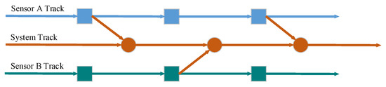
Figure 1.
Distributed fusion structure of multiple sensors.
2.2. Residual Network
He et al. [52] proposed a residual network consisting of a series of basic residual blocks. The residual network is very effective in solving the problems of gradient disappearance and gradient explosion, and can ensure better performance of the network even when the depth of the network increases. The basic residual module is shown in Figure 2a, which can be expressed as [53]
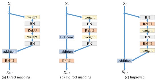
Figure 2.
Three different residual modules: (a) Direct mapping residual module; (b) indirect mapping residual module; (c) improved residual module.
The residual block consists of two parts: direct mapping and residual mapping. The left part of Figure 2a is direct mapping; the right part of Figure 2a is the residual part , which generally includes 2 or 3 convolutional layers. If the dimensions of input and output are different, it is necessary to use the 1 × 1 convolution operation to reduce or increase the dimension of the input, which is as shown in Figure 2b and can be expressed as [53]
where is the skip connection part and is the 1 × 1 convolution kernel.
If the network uses n residual modules, then the corresponding relationship between input and output can be expressed as [53]
Moreover, the gradient of the layer is transmitted to any other layer, and information transmission between the upper layer and the lower layer is realized [53].
The location of the activation function in the network will also affect the performance of the residual network. He et al. [53] improves the residual network and proves that the residual module of the structure shown in Figure 2c has the best performance. This structure puts the batch normalization (BN) and ReLU activation function before the convolution operation. Further, the activation function of the second layer moves from the addition operation to the residual part.
3. Methods
Activated by the advantages of distributed architecture and the residual module, we propose a new three-branch distributed fusion framework of MS and PAN images based on the residual module, RDFNet. The processes of fusion on LRMS and PAN images are roughly divided into four steps:
- MS and PAN images fed into RDFNet need to be preprocessed. Due to the different levels of remote sensing data obtained by different researchers, different preprocessing operations are also needed for remote sensing images; for example, radiometric correction including radiometric calibration and atmospheric correction, registration, and so forth. On account of the Landsat-8 and Landsat-7, the obtained data is L1T level, which has finished geometric accurate correction and radiometric correction; we only register the data following [54,55]. The GF-2 data is the 2A level, which has finished primary geometric correction and radiometric correction, so we carry out geometric accurate correction for it to make use of ENVI. QuickBird data is used as a standard product, and then we carry out geometric accurate correction for it to make use of ENVI. GF-2 and QuickBird data are registered with the same method as Landsat-8.
- The LRMS and PAN images are fused to generate the HRMS images. In fact, there are no MS images with the same spatial resolution as the fused HRMS images. Consequently, according to Wald’s protocol [56], the original-scale MS and PAN images are downsampled, denoted as DLMS and LPAN images, respectively; the specific process is shown in Figure 3. According to the resolution of MS and PAN images, the scaling factor is determined. As the size of MS and PAN images fed into RDFNet has to be kept the same, it is necessary to interpolate DLMS images to the size of LPAN image. Therefore, the original MS images can be used as ground truth.
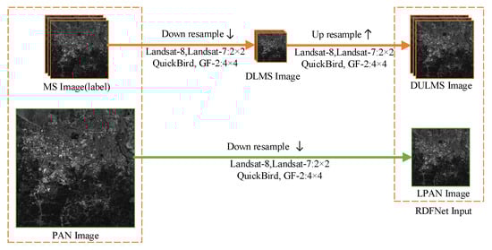 Figure 3. Workflow of generating training datasets according to Wald protocol.
 - The DULMS and LPAN images are fed into RDFNet, and the original MS images are the output of RDFNet, as shown in Figure 4. DULMS, LPAN, and MS images are randomly cropped 64 × 64 subimages to form training samples. By adjusting the super parameters and structure of the network, and after sufficient training, the optimal network is obtained. As shown in Figure 5 and Figure 6, the parameters of the well-trained network are then frozen and the performance of the network is tested on reduced-resolution and full-resolution MS and PAN images, respectively.
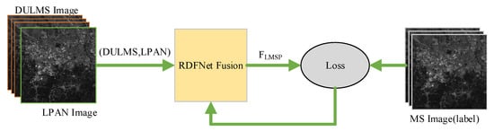 Figure 4. Training workflow of proposed RDFNet.
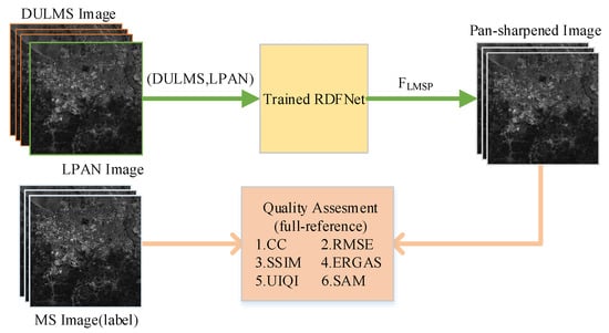 Figure 5. Testing and evaluating RDFNet with DULMS and LPAN images with reduced resolution.
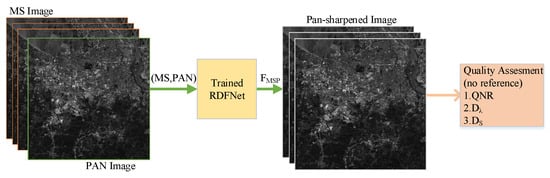 Figure 6. Testing and evaluating RDFNet with MS and PAN images with full resolution.
 - Eventually, the pan-sharpened images with reduced resolution are evaluated subjectively and quantitatively with the original MS images, making use of the full-reference metrics mentioned in Section 4.2, as shown in Figure 5. Additionally, the full-resolution, pan-sharpened images are evaluated subjectively and quantitatively, making use of the no-reference metrics mentioned in Section 4.2, as shown in Figure 6. Proceeding to the next step, the pan-sharpening performance of the proposed network is verified by analyzing the indicators and by subjective visual evaluation.
3.1. Overall Structure
Activated by the advantages of distributed architecture and the residual module, we propose a new three-branch distributed fusion framework of MS and PAN images based on the residual module, RDFNet. In the pan-sharpening of remote sensing images, the information collected by the MS and PAN sensors can be used simultaneously. Not only are the MS and PAN images under the current scale fused, but also the fused image of the previous different scale is fused. In this way, multiscale information is fully utilized to improve the accuracy of the generated HRMS image; the proposed RDFNet’s overall framework of pan-sharpening is as shown in Figure 7. From the perspective of mathematical theory, the fusion process is shown as follows.
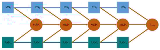
Figure 7.
The overall framework for MS and PAN images pan-sharpening.
The proposed fusion structure consists of three branches: MS features extraction, PAN features extraction, cross-scale fusion.
The MS features extraction branch can be defined as
where is the LRMS image and is the MS input of the fusion network. is other representations of after the residual module. means the residual module acting on the . represents MS images at different scales, which represent the features of different levels of , where is the lowest level feature and is the highest level feature. Different scale features of the spectral image are fused at each layer, which can make the best of each scale information of MS images. This means the method expresses more MS information so as to reduce spectral distortion.
The PAN features extraction branch can be defined as
where is the high-spatial-resolution PAN image and is the PAN input of fusion network. is other representations of after the residual module. means the residual module acting on the . denotes high-resolution PAN images at different scales, which represent different feature levels of , where is the lowest level feature and is the highest level feature. Different scale features of the PAN image are fused at each layer, which can make the best of each scale information of PAN image. As a result, the method expresses more spatial details so as to improve the spatial resolution of the fused image.
The cross scale fusion branch can be defined as
where , , , and are the fusion results of different levels. is equal to the fusion rule. They are the fusion results of the , of ith feature extraction layer, and the different scales of th fusion layer . In this way, it realizes cross-layer fusion. It can make better use of the local information of multisource images and then reduce the information loss in the convolution process.
3.2. Network Structure
The pan-sharpening model RDFNet proposed in this paper is composed of three branches; the RDFNet structure is shown in Figure 8. The two branches are used to extract the features of MS and PAN images, respectively. The last branch is used to fuse the features of the two branches and the fusion results of the previous step, layer by layer, until the last layer generates the pan-sharpened image. The first branch is for multiscale feature extraction of MS images. Four residual modules REM1, REM2, REM3, and REM4 are used to process the MS images so as to extract the multiscale features, as shown in the left of Figure 8. The third branch is used for multiscale feature extraction of PAN images. The four residual modules REP1, REP2, REP3, and REP4 are used to process the PAN images so as to extract the multiscale features, as shown on the right of Figure 8. The second branch is used for fusion, which is composed of FMP1, FMP2, FMP3, FMP4, and FMP5 modules; FMP5 module is the last convolution layer. It realizes the fusion of the two branches’ multiscale MS images, PAN image, and the fusion result of the previous layer, as shown in the middle part of Figure 8. For the sake of preserving the spectral information of the MS images and the spatial details of the PAN images as much as possible, the network uses full convolution instead of pooling. As pooling will miss some information, which may cause spectral distortion as well as texture and detail loss. RDFNet is equivalent to a powerful fusion function, in which the LRMS image and PAN image are input, and HRMS image is output.
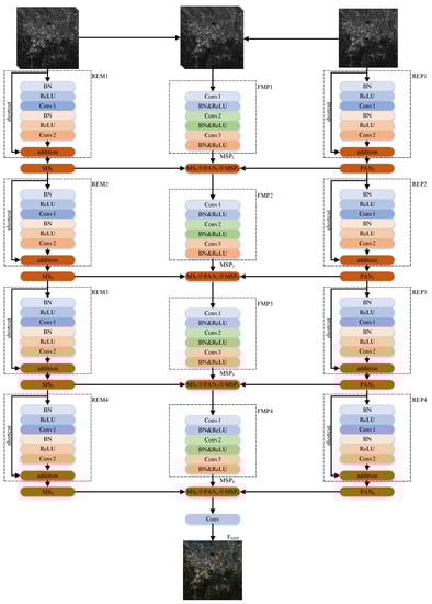
Figure 8.
Proposed RDFNet for pan-sharpening. RDFNet is divided into three branches. The left branch is for multiscale feature extraction of MS image. The right branch is the multiscale feature extraction branch of PAN image. The middle branch is used for fusion of the two branches.
Each module of the MS images features extraction branch can be expressed as follows:
REMi module:
where is the input of REMi module; is the output of REMi module; indicates the skip connection; * represents the convolution operation; is the REMi module convolution kernel, the size of which is 1 × 1, and the number of convolution kernels is 32, 64, 128, 256 in the skip connection, respectively. This operation is used to increase dimension and transfer information across scales. represents the residual part; is the convolution kernel; the size of the convolution kernel is 3 × 3, and there are 32, 64, 128, 256 convolution kernels in the residual part, respectively.
Then, the feature extraction branch of MS images can be expressed as
where is the output of the ith residual module. It can be seen from the expression that the cross-layer transmission of information is realized, which is related to the residual part of residual module.
Each module of the PAN image features extraction branch can be expressed as follows:
REPi module:
where is the input of REPi module; is the output of REPi module; is the REPi module convolution kernel, the size of which is 1 × 1, and the number of convolution kernels is 32, 64, 128, 256 in the skip connection, respectively. This operation is used to increase dimension and transfer information across scales. represents the residual part; is the convolution kernel; the size of the convolution kernel is 3 × 3, and there are 32, 64, 128, 256 convolution kernels in the residual part, respectively.
Then, the feature extraction branch of PAN image can be expressed as follows:
where is the output of the ith residual module.
The operation of each part of fusion branch can be expressed as follows:
FMPi module:
where is the result of the fusion module FMPi, is the fusion result of FMP5 module and the whole network. () is the input of the FMPi module, which represents the concatenated images , , and on the channel. () is the 1 × 1 convolution kernel and there are 32, 64, 128, 256 convolution kernels at each fusion layer, respectively. is the 1 × 1 × 3 convolution kernel of the last fusion layer. is equivalent to the fusion function.
RDFNet can generate a powerful remote sensing image fusion model after sufficient training of samples. In order to improve the accuracy of the RDFNet, the residual module uses the combination mode with higher accuracy. First, BN is performed; then, nonlinear operation is carried out using the ReLU activation function; finally, the convolution operation is performed. Different from the conventional residual module, the last layer of ReLU activation function is moved from the addition operation to the residual part. In the fusion module, the 1 × 1 convolution layer is used to realize multichannel information fusion, and the ReLU activation function is used to increase the nonlinearity and improve the fusion ability of the fusion model. The fusion model of the whole RDFNet can be expressed as ; is the fusion model.
3.3. Loss Function
Assuming that the input of the network is LM and the ideal fusion result is HM (label), then the training samples of the network can be expressed as , where N is the total number of training samples. Then, the training process of the fusion network is to find the fusion model , where is the prediction output, that is, the actual output of the fusion network. The process of training the fusion function is actually the problem of the regression function. The mean square error (MSE) is chosen as the loss function of the network.
where m is the batch size, that is, the number of training samples used in each iteration. In the process of training, Adam optimizer [57] is used to optimize the loss function, that is, the minimum value of LF is obtained. During the optimization process, the weights are updated as follows.
where is the exponential moving averages of the gradient, is the squared gradient, and are the bias-corrected estimates, represents the previous time, t represents the current time, a is the learning rate, the initial iteration is set to , and a is set reasonably according to the number of iterations so that the learning rate in the later stage is not too low. The exponential decay rate of first-order moment estimation is set to 0.9 and second-order moment estimation is set to 0.999. is a very small value, ensuring that the denominator is not 0, set to .
4. Experimental Results and Analysis
4.1. Study Area and Datasets
The datasets are divided into training datasets and testing datasets. The data of the Landsat-8 satellite are used as the training datasets. In order to verify the fusion performance of RDFNet, the data of Landsat-8, Landsat-7, QuickBird, and GF-2 satellites are used as the testing datasets. The Landsat-8 and Landsat-7 data download address is https://glovis.usgs.gov/ (accessed on 3 March 1879).
Landsat-8 carries two sensors: Operational Land Imager (OLI) and Thermal Infrared Sensor (TIRS). OLI has nine bands, of which the spatial resolution of bands is 1–7, 9 is 30 m, and band 8 is panchromatic band with 15 m spatial resolution. TIRS consists of 10 band and 11 band. The band range is shown in Table 1. In this paper, 4, 3, and 2 bands are used as R, G, and B channels, respectively.

Table 1.
Satellite parameters.
The Landsat-7 satellite carries an Enhanced Thematic Mapper (ETM+) with a total of eight bands, among which the resolution of 1, 2, and 3 bands is 30 m, and the resolution of 8-band is 15 m. As shown in Table 1, we use the 3, 2, and 1 bands of the multispectrum as the R, G, and B channels, respectively.
The resolution of the PAN image of QuickBird satellite products is 0.61–0.72 m, and the spatial resolution of the MS image is 2.44–2.88 m. The resolution of the images we used is 0.7 m and 2.8 m, as shown in Table 1.
GF-2 satellite products have a total of five bands. The resolution of PAN image is 1 m, and the spatial resolution of MS image is 4 m. In this paper, 4, 3, and 2 bands of multispectrum are used as R, G, and B channels, respectively, as shown in Table 1.
4.1.1. Training Datasets
We use two Landsat-8 image pairs in total, the first and left half of the second images are used as training data, and the right half of the second image is used as testing data. The sizes of the two MS images are 4584 × 4674 and 4566 × 4644, respectively, and the corresponding PAN images sizes are 9168 × 9348 and 9132 × 9288. One of the training datasets is shown in Figure 9 (For better typesetting, the size of MS and PAN images are shown as the same size even when they have different resolutions in actuality.). The images are obtained by the Landsat-8 satellite sensors. The corresponding date of the remote sensing images is 6 May 2020. The corresponding area is near the South Bay in Haikou City, Hainan Province, where Figure 9a is the MS image with a resolution of 30 m and pixel size of 600 × 600; Figure 9b is the PAN image with a resolution of 15 m and pixel size of 1200 × 1200. As there are no MS images with a spatial resolution of 15 m in the actual collected data, in order to verify the fusion performance of the proposed network RDFNet, we follow Wald’s criterion [56] to downsample the remote sensing images to obtain simulated images.

Figure 9.
Training datasets of Landsat-8 near the South Bay in Haikou City, Hainan Province. (a) MS image with 30 m spatial resolution; (b) PAN image with 15 m spatial resolution.
According to the bicubic resampling method [58], the PAN image with spatial resolution of 15 m is downsampled to 30 m; the MS images with spatial resolution of 30 m are also downsampled to 60 m. In this way, the downsampled PAN image with a spatial resolution of 30 m and the MS images with spatial resolution of 60 m can be fused to obtain the MS images with spatial resolution of 30 m. The fused MS images obtained by the RDFNet are compared with the 30 m MS images obtained in reality (the ideal output image of the network). Then, the performance of the fusion network is evaluated. As the input of the network needs to maintain the same size, it is also necessary to perform an upsampling operation on the MS images with a spatial resolution of 60 m to obtain the MS images with the same size as the PAN image with spatial resolution of 30 m. As the size of the input network is different, subimages are randomly cropped from the preprocessed images as training datasets. We simulate 20,688 image pairs using Lansat-8 images for training and 5172 image pairs for validating the fusion network.
4.1.2. Testing Datasets
In order to verify the generalization ability and fusion performance of the RDFNet proposed in this paper, four different satellites’ data are used for experiments. In order to better illustrate that the proposed network can fuse different sizes of images, the size of the testing data we employed is different from that of the training data. Some testing datasets are shown in Figure 10 (For better typesetting, the size of MS and PAN images are shown as the same size even when they have different resolutions in actuality.). There are four different regions of different satellites.
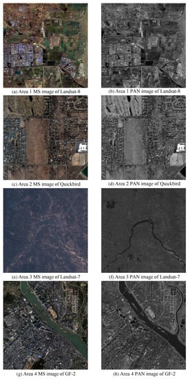
Figure 10.
Testing datasets of four different satellites: (a) Area 1 MS image with 30-m resolution of Landsat-8. (b) Area 1 PAN image with 15-m resolution of Landsat-8. (c) Area 2 MS image with 2.8-m resolution of QuickBird. (d) Area 2 PAN image with 0.7-m resolution of QuickBird. (e) Area 3 MS image with 30-m resolution of Landsat-7. (f) Area 3 PAN image with 15-m resolution of Landsat-7. (g) Area 4 MS image with 4-m resolution of GF-2. (h) Area 4 PAN image with 1-m resolution of GF-2.
Area 1 images are acquired by the Landsat-8 satellite sensors as a part of testing data. This testing data comes from the right side of the second image in Section 4.1.1. There is no overlap between area 1 and the training datasets, as shown in Figure 10a,b. The remote sensing images were acquired on 15 June 2017 at an area near Bohai Bay in Cangzhou City, Hebei Province. Figure 10a shows the corresponding MS image with a spatial resolution of 30 m and pixel size of 600 × 600. Figure 10b shows the corresponding PAN image with a spatial resolution of 15 m and pixel size of 1200 × 1200. According to Wald’s criterion, the 15-m PAN and 30-m MS images are downsampled by a factor of 2 to obtain 30-m PAN and 60-m MS simulation images, respectively. We simulated 55 testing image pairs for Landsat-8.
Images of area 2 are some testing datasets obtained by QuickBird satellite, located in the Inner Mongolia Autonomous Region, as shown in Figure 10c,d. Figure 10c is the MS images with a spatial resolution of 2.8 m and pixel size of 510 × 510. Figure 5d is the corresponding PAN image with a resolution of 0.7 m and pixel size of 2040 × 2040. According to Wald’s criterion, the PAN and MS images are downsampled by a factor of 4 to obtain 2.8 m PAN and 11.2 m MS simulation images, respectively. We simulated 48 testing image pairs for QuickBird.
Area 3 is a part of image pairs of Haikou City, Hainan Province, near the South China Sea, acquired by the Landsat-7 satellite on 8 November 2000, as shown in Figure 10e,f. Figure 10e is the MS image with a spatial resolution of 30 m and pixel size 600 × 600. Figure 10f is the corresponding PAN image with a spatial resolution of 15 m and pixel size 1200 × 1200. According to Wald’s criterion, the PAN and MS images are downsampled by a factor of 2 to obtain 30 m PAN and 60 m MS simulation images, respectively. We simulated 50 testing image pairs for Landsat-7.
Area 4 is the partial images of Haikou City, Hainan Province acquired by the GF-2 satellite sensors on 9 December 2016, as shown in Figure 10g,h. Figure 10g is the MS image with a spatial resolution of 4 m and pixel size of 785 × 822. Figure 10h is the corresponding PAN image with a resolution of 1 m and pixel size of 3140 × 3288. According to Wald’s criterion, the PAN and MS images are downsampled by a factor of 4 to obtain 4 m PAN and 16 m MS simulation images, respectively. We simulated 45 testing image pairs for GF-2.
4.2. Fusion Quality Metrics
The final fusion results are evaluated by subjective visual perception and objective metrics. Subjective visual perception evaluation is used to compare the fusion result, reference image, and the original image with human vision and observe the clarity, color, outline, and some details, then to judge whether the fusion effect is good or bad. Subjective visual perception evaluation will vary from person to person, and can only represent the judgment results of certain people, which is somewhat one-sided. A reliable, quantitative, and objective quality metric is also needed to further analyze the fusion results to determine the fusion effect. Among them, the following objective quality indicators are mainly used to evaluate the fusion results, which can be divided into full-reference and no-reference indicators. The full-reference indexes we use include correlation coefficient () [56], Root Mean Square Error () [59], Structural similarity () [60], Spectral angle mapping () [61], Erreur Relative Globale Adimensionnelle de Synthése () [14], and universal image quality index () [62]. The no-reference indexes we use consist of , , [63].
The definition of [56] of images T and F is expressed as
where is the similarity index, T is the reference image, and F is the fused image. represents the spatial similarity of images T and F, and the value of is between [−1,1]. The image size of T and F is . is the covariance of T and F, is the standard deviation of T, is the standard deviation of F, represents the mean value of image T, represents the mean value of image F if and only if , —that is, if the T and F images are more similar, the corresponding is closer to 1. Therefore, the closer the is to 1, the better the corresponding fusion effect.
[59] is defined as
represents the difference degree of pixels between the fused image F and the reference image T, and it is the evaluation metric of spatial detail information if and only if , , so the ideal value of is 0. The smaller the , the smaller the difference between the fusion image and the reference image and the better the fusion effect.
[60] is expressed as
Generally, is the covariance of image T and F, is the variance of the image T, and is the variance of image F. For the sake of preventing the denominator from being 0, , , and are constants; L is the dynamic range of pixel values; ; and . ; then, we can obtain the equation of .
In each calculation, we take a window from the image, and then slide the window continuously for calculation. Finally, we take the average value as the global . For MS images, is calculated in different bands and the average value is taken. is a number between 0 and 1. The larger the , the smaller the difference between the fused image and the reference image—that is, the better the image quality. When two images are such as two peas, .
[61] considers the spectrum of a pixel as a vector and measures the similarity of the spectrum by calculating the angle between two vectors. The more similar the fusion spectrum is to the reference spectrum, the better the corresponding fusion effect. The mathematical expression is defined as
where is the spectral vector of the reference image and is the spectral vector of fused image. When and only when , . The closer the is to 0, the smaller the degree of spectral distortion and the better the fusion effect.
[14] is mainly used to calculate the degree of spectral distortion, and its expression is defined as
Among them, represents the spatial resolution of PAN image, represents the spatial resolution of MS image, is the root mean square error of the ith band of the reference image and the pan-sharpened image, represents the average value of the ith band of the reference image. The smaller the value, the better the fusion effect.
[62] is used to estimate the similarity between images T and F, and its expression is defined as
If and only if , . Therefore, the more similar T and F are, the closer the Q value is to 1, and the better the spectral quality of the corresponding fused image.
Quality with no-reference () metric [63] is introduced on the basis of . For pan-sharpening evaluation, it does not need the ideal output as the reference metric. It includes two indexes: spectral distortion and spatial distortion.
Spectral distortion is represented as , which is related to LRMS image and fusion image, the formula is expressed as
Among them, expresses the lth band of the LRMS image, means the rth band of the fused image, B is the number of bands, and p is a positive integer for amplifying the spectral difference—the default is 1.
Spatial distortion is represented by , which is related to the LRMS image, PAN image, and fusion image. Its formula is expressed as
where P is PAN image and is the PAN image degraded from P to LRMS image resolution. The expression of is defined as
The smaller the degree of spectral distortion and spatial distortion between the fusion image, LRMS image, and PAN image, the larger the corresponding value.
4.3. Implementation Details
The datasets are divided into a training dataset, Landsat-8, and testing datasets, Landsat-8, Landsat-7, QuickBird, and GF-2. According to Wald’s protocol, the obtained degraded LPAN and DULMS images of the training dataset Landsat-8 are randomly cropped; the subimage size is 64 × 64 and augments the subimage with rotation. Experiments of RDFNet fusion model are performed on a TensorFlow hardware setup with an Intel Xeon CPU, a NVIDIA Tesla V100 PCIE GPU, and 16 GB RAM.
4.4. Simulation Datasets Experimental Results
In this section, we employ the current mainstream remote sensing image pan-sharpening methods compared with RDFNet proposed in this paper so as to demonstrate the RDFNet fusion performance on the reduced resolution of training and testing datasets, including widely used traditional methods and CNN-based methods. The eight comparison methods we used are as follows: Brovey [7], GS [1], SFIM [19], IFCNN [64], PNN [36], DRPNN [39], PanNet [40], ResTFNet [45]. The parameters of these methods are set according to the literature. The URLs of IFCNN, PNN, DRPNN, PanNet, and ResTFNet code are github.com/uzeful/IFCNN (accessed on 6 November 2019), www.grip.unina.it (accessed on 1 January 2016), github.com/Decri (accessed on 19 May 2018), github.com/oyam/PanNet-Landsat (accessed on 10 February 2020), github.com/liouxy/tfnet (accessed on 12 December 2017 and we change it according to [45]), respectively. In order to evaluate the performance of RDFNet, we employ several full-reference indexes proposed in the literature. For instance, CC [56], RMSE [59], SSIM [60], UIQI [62], SAM [61], ERGAS [14].
The fusion results of the Landsat-8 training data are shown in Figure 11; the objective evaluation metrics of the fusion results are calculated and the corresponding bar chart is shown in Figure 12. Figure 11a is the degraded MS image with a spatial resolution of 60 m (The size of LRMS is the same as PAN and fused images even when they have different resolutions in actuality.). Figure 11b is the degraded PAN image with a spatial resolution of 30 m. Figure 11c is the only upsampled MS image by Figure 11a. Figure 11m is the MS image collected with a spatial resolution of 30 m, namely, the ground truth. Figure 11d–k are the Brovey, GS, SFIM, IFCNN, PNN, DRPNN, PanNet, and ResTFNet fusion results with spatial resolutions of 30 m, respectively, which are obtained by fusing Figure 11a,b. Figure 11l is the proposed RDFNet fusion result with a spatial resolution of 30 m. In order to better subjectively evaluate the fusion effect, the red box area in the figures is enlarged, as shown in the red box in the lower right corner of the figures.
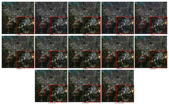
Figure 11.
Subjective visual comparison between RDFNet and the current mainstream fusion methods for the testing dataset fusion results of Landsat-8 with reduced resolution. (a) LRMS; (b) PAN; (c) Bicubic; (d) Brovey; (e) GS; (f) SFIM; (g) IFCNN; (h) PNN; (i) DRPNN; (j) PanNet; (k) ResTFNet; (l) RDFNet (ours); (m) ground truth.
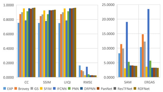
Figure 12.
Quantitative evaluation metrics of the Landsat-8 training dataset with reduced resolution.
Through careful observation of the pan-sharpening results shown in Figure 11 and Figure 12, these methods can improve the spatial resolution, but the degree of improvement is not the same, and there is some spectral distortion. From Figure 12, we can see that the proposed RDFNet achieves the best performance on the basis of all indexes, except SAM, which is second only to SFIM. For CC and SSIM, RDFNet method is the best, which shows that this method extracts more details. Although the metric SAM of RDFNet is a little bigger than SFIM, it is smaller than any other method, and ERGAS is the smallest of the comparison methods. The quality of pan-sharpening is further improved by establishing the network with three branches and a residual module, especially reducing spectral distortion and preserving spatial details. Bicubic interpolation is represented by EXP [44,54,55] and no details are injected. Numerical results show that the performance of IFCNN is the worst. As the IFCNN network is a general fusion model, the fusion network is not sensitive to remote sensing images because of the unique MS and PAN information of remote sensing images. We can clearly see that the performance of PNN is very different from DRPNN. The network using residual is obviously better than PNN in preserving both spectral information and spatial details. DRPNN and PanNet have similar performance. The performance of ResTFNet is better than that of DRPNN and PanNet, the success of which is attributed to the feature extraction of MS and PAN images by two branches. Interestingly, we found that the proposed RDFNet performance is superior to ResTFNet. This is because the proposed RDFNet with the three branches fusion structure can make full use of the spectral information and spatial structure, so as to reduce the spectral distortion and the loss of spatial details.
From Figure 11, we can find that all the methods produce visually clearer pan-sharpened images than LRMS. The pan-sharpened image generated by the proposed method is very similar to the ground truth image in terms of vision. The spatial information is well preserved, and there is no noticeable ringing phenomenon and spectral distortion. The EXP image is very blurry. Brovey and GS can significantly improve the spatial resolution, but there are problems of oversharpening and spectral distortion. Although SFIM can suppress the oversharpening problem, it will cause the fusion result to be blurred and the spectrum to be slightly distorted. The fusion result of IFCNN gives rise to serious spectral distortion, and the image is vague. The spectral distortion of PNN is reduced, but there are problems of blur and ringing effects. DRPNN improves the definition slightly on the basis of PNN. In fact, the residual-based pan-sharpening effects of DRPNN, PanNet, ResTFNet, and RDFNet are quite good; however, we can find that the RDFNet pan-sharpened image is closest to the ground truth. In more detail, the buildings in the red box of the PanNet result have the greatest color contrast, followed by ResTFNet and DRPNN, while RDFNet is the closest to the reference image. The RDFNet method can ensure higher spatial resolution; simultaneously, it has the least spectral and spatial distortion, so the fusion performance of the fusion network proposed in this paper is superior.
In order to better represent the difference between the pan-sharpened MS image and the ground-truth MS image, the average intensity difference maps and the average spectral difference maps [65] between the pan-sharpened MS image and the ground-truth MS image are given in Figure 13. The color map is used to represent the difference value of the comparison methods. The color bar is at the bottom of Figure 13, and the value increases gradually from left to right. The top row are the average intensity difference maps of the whole image; the second row are the average intensity difference maps of the enlarged area in Figure 11; the third row are the average spectral difference maps of the whole image; and the bottom row are the average spectral difference maps of the enlarged area in Figure 11. In the top row of Figure 13, it can be seen that the difference of the proposed method is the smallest. The difference of Brovey is greatest in Figure 13a. In the second row of Figure 13, it can be seen that the difference shown by the proposed method is smallest. The great differences are shown in Figure 13a Brovey, Figure 13b GS, and Figure 13d IFCNN; these methods have serious spectral distortion. Figure 13c displays SFIM. Although SFIM retains the spectral information, the detail information is lost; hence, its spatial resolution is relatively low. It can be observed from Figure 13e–h—PNN, DRPNN, PanNet, and ResTFNet, respectively—that, the spectral information of ResTFNet is well preserved and more details are extracted. However, the spectral distortion and spatial distortion of the proposed method, RDFNet (Figure 13i), are lower.

Figure 13.
Average intensity difference maps and average spectral difference maps between a pan-sharpened MS image and ground-truth MS image for the Landsat-8 training dataset with reduced resolution; the top row are the average intensity difference maps of the whole image, the second row are the average intensity difference maps of the enlarged area in Figure 11, the third row are the average spectral difference maps of the whole image, and the bottom row are the average spectral difference maps of the enlarged area in Figure 11. (a) Brovey; (b) GS; (c) SFIM; (d) IFCNN; (e) PNN; (f) DRPNN; (g) PanNet; (h) ResTFNet; (i) RDFNet (ours).
In order to verify the performance of the proposed RDFNet, we carried out a lot of experiments on low resolution and full resolution, respectively, using MS and PAN images of four different satellites, including Landsat-8, QuickBird, Landsat-7, and GF-2. This section is used to present the degraded resolution fusion results.
The degraded resolution experimental results of the Landsat-8 testing data are shown in Figure 14. The representation of each image is the same as that in Figure 11. The average intensity difference maps and the average spectral difference maps are shown in Figure 15. It can be seen from Figure 14 that the proposed method is closer to the ground truth image. Figure 15i also shows the smallest difference. It can be seen from Figure 14 that compared with ground truth, Brovey and GS (Figure 14d,e) fusion results are oversharpened, and there is spectral distortion. The corresponding images in Figure 15a,b show a relatively large intensity difference and spectral difference. We also observe in Figure 14g that IFCNN apparently loses much spectral information, and its spectral difference and detail information difference are relatively large in Figure 15d. In Figure 14f, although there is less spectral distortion of SFIM fusion results, the spatial resolution improvement is lower, and the fusion images look vague compared with the ground truth images. In Figure 14h–l, comparing the fusion results of PNN, DRPNN, PanNet, ResTFNet, and RDFNet with the ground truth image, we can see that the spectral fidelity of these methods is fairly good. However, we can see in the difference from color maps of Figure 15 that RDFNet retains the best spectral and structural information, followed by ResTFNet.
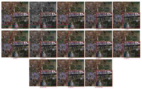
Figure 14.
Subjective comparison between RDFNet and the current mainstream fusion methods for testing dataset fusion results of Landsat-8 with reduced resolution. (a) LRMS; (b) PAN; (c) Bicubic; (d) Brovey; (e) GS; (f) SFIM; (g) IFCNN; (h) PNN; (i) DRPNN; (j) PanNet; (k) ResTFNet; (l) RDFNet (ours); (m) ground truth.
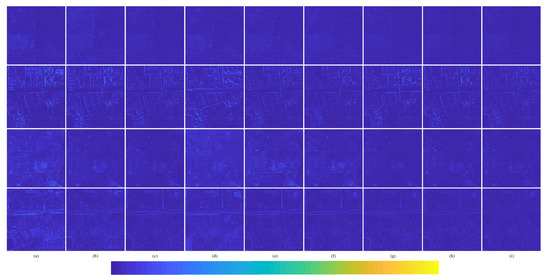
Figure 15.
Average intensity difference maps and average spectral difference maps between the pan-sharpened MS image and ground-truth MS image for the Landsat-8 testing dataset with reduced resolution; the top row are the average intensity difference maps of the whole image, the second row are the average intensity difference maps of the enlarged area in Figure 14, the third row are the average spectral difference maps of the whole image, and the bottom row are the average spectral difference maps of the enlarged area in Figure 14. (a) Brovey; (b) GS; (c) SFIM; (d) IFCNN; (e) PNN; (f) DRPNN; (g) PanNet; (h) ResTFNet; (i) RDFNet (ours).
The degraded resolution experimental results of QuickBird testing data are shown in Figure 16. The average intensity difference maps and the average spectral difference maps are shown in Figure 17. The QuickBird has only four bands, but the spectral range of visible light is very similar to that of Landsat-8. It can be seen from Figure 16 that the proposed method is closer to the reference image in terms of spectral information and clarity. Figure 17i also shows that the proposed method RDFNet retains much more spectral and structural information. The spectral distortions of Figure 17a Brovey, Figure 17b GS, Figure 17d IFCNN, and Figure 17e PNN are more serious, and the severity is less in turn. From Figure 17f–i, comparing the fusion results of DRPNN, PanNet, and ResTFNet with RDFNet, we observe that the spectral fidelity of RDFNet is fairly good and preserves more details.
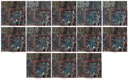
Figure 16.
Subjective comparison between RDFNet and the current mainstream fusion methods for testing dataset fusion results of QuickBird with reduced resolution. (a) LRMS; (b) PAN; (c) Bicubic; (d) Brovey; (e) GS; (f) SFIM; (g) IFCNN; (h) PNN; (i) DRPNN; (j) PanNet; (k) ResTFNet; (l) RDFNet (ours); (m) ground truth.

Figure 17.
Average intensity difference maps and average spectral difference maps between the pan-sharpened MS image and ground-truth MS image for the QuickBird testing dataset with reduced resolution; the top row are the average intensity difference maps of the whole image, the second row are the average intensity difference maps of the enlarged area in Figure 16, the third row are the average spectral difference maps of the whole image, and the bottom row are the average spectral difference maps of the enlarged area in Figure 16. (a) Brovey; (b) GS; (c) SFIM; (d) IFCNN; (e) PNN; (f) DRPNN; (g) PanNet; (h) ResTFNet; (i) RDFNet (ours).
The degraded resolution experimental results of Landsat-7 testing data are shown in Figure 18. The average intensity difference maps and the average spectral difference maps are shown in Figure 19 and Figure 20. In Figure 19, the top row are the average intensity difference maps of the whole image, the second row are the average spectral difference maps of the whole image. In Figure 20, the top row are the enlarged views of the yellow box in Figure 18, the middle row are the intensity difference maps of the enlarged area of the yellow box in Figure 18, and the bottom row are the spectral difference maps of the enlarged area of the yellow box in Figure 18. Obviously, it can be observed from Figure 18 and Figure 19 that the proposed fusion model RDFNet is much better for both improving spatial resolution and retaining spectral information. Figure 20 shows an enlarged view of the river branch. From the details, we can clearly distinguish the difference of each comparison method in retaining spectral information and spatial information. Figure 20b GS and Figure 20d IFCNN lose much more spectral information. In Figure 20c SFIM and Figure 20e PNN, there are no differences in the top row, but if we look at the middle row and the bottom row, we find that SFIM retains more spectral information and slightly less detail. The fusion performance of Figure 20f DRPNN, Figure 20g PanNet, and Figure 20h ResTFNet are good for reducing spectral distortion and retaining details, but ResTFNet is better. However, the proposed fusion method RDFNet has superior performance.
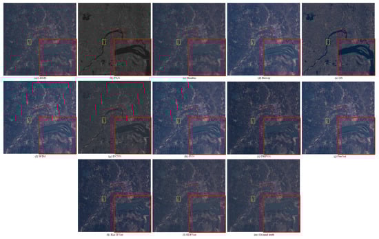
Figure 18.
Subjective comparison between RDFNet and the current mainstream fusion methods for testing dataset fusion results of Landsat-7 with reduced resolution. (a) LRMS; (b) PAN; (c) Bicubic; (d) Brovey; (e) GS; (f) SFIM; (g) IFCNN; (h) PNN; (i) DRPNN; (j) PanNet; (k) ResTFNet; (l) RDFNet (ours); (m) ground truth.

Figure 19.
Average intensity difference maps and average spectral difference maps between pan-sharpened MS image and ground-truth MS image for testing dataset Landsat-7 with reduced resolution; the top row are the average intensity difference maps, the bottom row are the average spectral difference maps. (a) Brovey; (b) GS; (c) SFIM; (d) IFCNN; (e) PNN; (f) DRPNN; (g) PanNet; (h) ResTFNet; (i) RDFNet (ours).
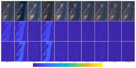
Figure 20.
Enlarged view of the yellow box in Figure 18, the corresponding average intensity difference maps, and the average spectral difference maps; the top row are the enlarged views of the yellow box in Figure 18, the middle row are average intensity difference maps, the bottom row are average spectral difference maps. (a) Brovey; (b) GS; (c) SFIM; (d) IFCNN; (e) PNN; (f) DRPNN; (g) PanNet; (h) ResTFNet; (i) RDFNet (ours); (j) ground truth.
The degraded resolution experimental results of GF-2 testing data are shown in Figure 21. The average intensity difference maps and the average spectral difference maps are shown in Figure 22. From Figure 21 and Figure 22, the spectral distortion of IFCNN, Brovey, and GS is still serious; however, compared with these three methods, the structure of IFCNN is closer to the ground truth. In comparison, the spectral information of SFIM is better preserved. However, the spatial information is a little sharpened and there are artifacts compared with the proposed pan-sharpened model RDFNet. From Figure 21h–l, comparing the fusion results of PNN, DRPNN, PanNet, and ResTFNet with the ground truth image, we can see that the spectral fidelity of these methods is fairly good. However, we can see from the difference of the color maps in Figure 22 that ResTFNet has less spectral distortion with a little sharpening. On the whole, the effect of the model proposed is better. In summary, compared with the aforementioned algorithms, the proposed RDFNet fusion result not only improves the spatial resolution, but also has less spectral distortion and almost no oversharpening.
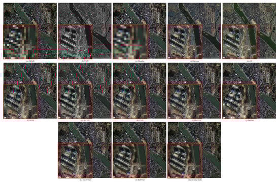
Figure 21.
Subjective comparison between RDFNet and the current mainstream fusion methods for testing dataset fusion results of GF-2 with reduced resolution. (a) LRMS; (b) PAN; (c) Bicubic; (d) Brovey; (e) GS; (f) SFIM; (g) IFCNN; (h) PNN; (i) DRPNN; (j) PanNet; (k) ResTFNet; (l) RDFNet (ours); (m) ground truth.

Figure 22.
Average intensity difference maps and average spectral difference maps between pan-sharpened MS image and ground-truth MS image for testing dataset GF-2 with reduced resolution; the top row are the average intensity difference maps of the whole image, the second row are the average intensity difference maps of the enlarged area in Figure 21, the third row are the average spectral difference maps of the whole image, the bottom row are the average spectral difference maps of the enlarged area in Figure 21. (a) Brovey; (b) GS; (c) SFIM; (d) IFCNN; (e) PNN; (f) DRPNN; (g) PanNet; (h) ResTFNet; (i) RDFNet (ours).
The objective evaluation indexes of fusion results on testing datasets are calculated, and the corresponding bar charts are shown in Figure 23, Figure 24, Figure 25 and Figure 26, respectively. From the value of each metric, the effect of RDFNet proposed in this paper is the best. It can be seen from the bar chart in Figure 23 that the indexes of CC, SSIM, and UIQI of the proposed method are the largest, while RMSE, SAM, and ERGAS are the smallest, respectively. This shows that the proposed method retains more spectral information while preserving spatial structure information, which is more conducive to providing better HRMS images. From the digital indicators in Figure 23, Brovey and GS have little difference, which is consistent with visual perception (Figure 14). However, the RMSE, SAM, and ERGAS numerical values of IFCNN are relatively large, and the fusion effect is not good. The fusion results of DRPNN and PanNet have similar digital indicators, which are better than PNN. Further, the digital index of ResTFNet fusion result is better than that of DRPNN and PanNet. In a word, the digital index of proposed RDFNet method is optimal. The indexes of other testing datasets are shown in Figure 24, Figure 25 and Figure 26. Similarly, it can be seen from bar charts (Figure 24, Figure 25 and Figure 26) that each evaluation index of the proposed method is optimal. Consequently, the fusion performance of the proposed RDFNet is the most outstanding. This shows that the proposed method can simultaneously improve the spatial resolution and retain the spectral information better. Although there is little difference with the existing methods, it improves the spatial resolution and retains more spectral information on the basis of the existing methods. This is of great significance to applications that require higher spatial resolution or higher spectral resolution, and has certain significance in practical applications.
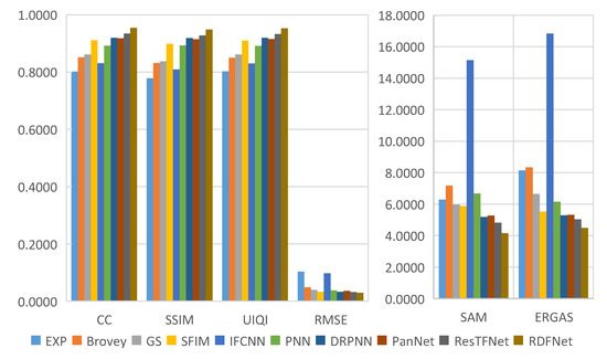
Figure 23.
Quantitative metrics of testing dataset fusion results on Landsat-8 with reduced resolution.
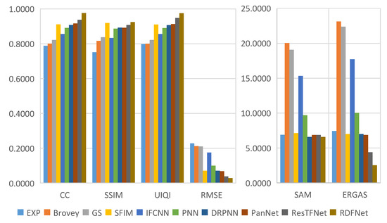
Figure 24.
Quantitative metrics of testing dataset fusion results on QuickBird with reduced resolution.

Figure 25.
Quantitative metrics of testing dataset fusion results on Landsat-7 with reduced resolution.

Figure 26.
Quantitative metrics of testing dataset fusion results on GF-2 with reduced resolution.
In order to comprehensively analyze the fusion performance of the network, Figure 27 shows the fusion time of the testing datasets on low resolution. In the future, we will employ the combination of extracting high-frequency information and deep network to explore the lighter fusion model.
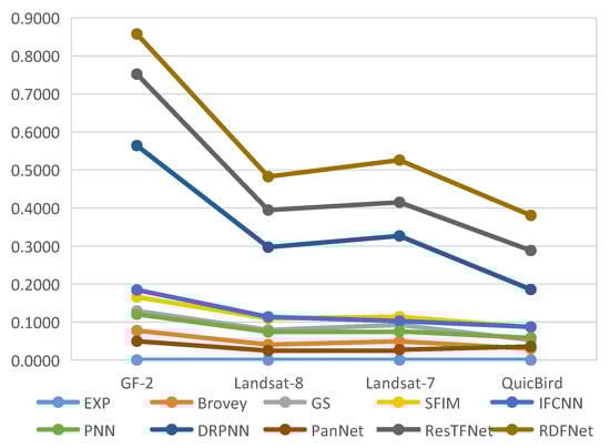
Figure 27.
All the CNN-based methods are implemented on a GPU, other methods are implemented on a CPU. Test time (s) of testing datasets with reduced resolution.
4.5. Full-Resolution Datasets’ Experimental Results
In this section, remote sensing data collected from Landsat-8, QuickBird, Landsat-7, and GF-2 are used for pan-sharpening. The visual perception comparison of mainstream methods on fusion results is shown in Figure 28, Figure 29, Figure 30 and Figure 31. Among them, ULMS is an upsampled MS image by the original MS image. From Figure 28, Figure 29, Figure 30 and Figure 31, we observe that the spatial resolution of all the fusion results is improved compared with ULMS. However, it can be seen from Figure 28 that fusion results of Brovey, IFCNN, and PanNet have obvious spectral distortion. By observing the fusion results of other methods corresponding to the two yellow regions of ULMS image, we find that the result of RDFNet is closer to the spectrum of ULMS image. In addition, ResTFNet is blurrier than RDFNet. From Figure 29, the resolution of all fusion results is improved. It can be seen that the SFIM, PNN, and DRPNN methods have the problems of blur and artifacts. Compared with ULMS, the Brovey, GS, IFCNN, and PanNet methods have obvious spectral distortion. Visually, compared with the luminance of ULMS image, the fusion result of ResTFNet is darker, while the fusion result of RDFNet is more consistent with the ULMS image. In Figure 30, the resolution of the fusion results of all methods is higher than that of ULMS. The fusion results of IFCNN and PanNet show serious spectral distortion. The fusion results of Brovey, GS, SFIM, PNN and DRPNN also show spectral distortion, but the color of Brovey, SFIM, PNN, and DRPNN are darker than that of ULMS, and the color of GS is lighter than that of ULMS. The fusion results of the ResTFNet method are better than the above methods, but compared with the fusion result of RDFNet method proposed, the fusion result of RDFNet method has higher resolution and preserves more spectral information. For Figure 31, compared with ULMS, the resolution of all fusion results is improved. However, Brovey, GS, and IFCNN all produce severe spectral distortion. In terms of SFIM, PNN, and PanNet, the fusion results are blurry and produce ringing artifacts. Relatively speaking, the fusion results generated by DRPNN, ResTFNet, and RDFNet are better. However, by carefully observation, we show that the fusion result of RDFNet is more accurate than ResTFNet and DRPNN. All in all, compared with these methods, the RDFNet proposed in the paper has higher spatial resolution and the least spatial and spectral distortion.
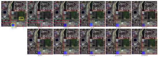
Figure 28.
Subjective comparison between RDFNet and the current mainstream fusion methods for fusion results on the Landsat-8 testing dataset with full resolution. (a) ULMS; (b) PAN; (c) Brovey; (d) GS; (e) SFIM; (f) IFCNN; (g) PNN; (h) DRPNN; (i) PanNet; (j) ResTFNet; (k) RDFNet (ours).
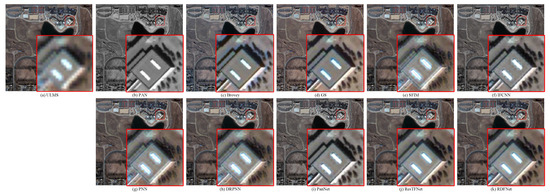
Figure 29.
Subjective comparison between RDFNet and the current mainstream fusion methods for fusion results on the QuickBird testing dataset with full resolution. (a) ULMS; (b) PAN; (c) Brovey; (d) GS; (e) SFIM; (f) IFCNN; (g) PNN; (h) DRPNN; (i) PanNet; (j) ResTFNet; (k) RDFNet (ours).
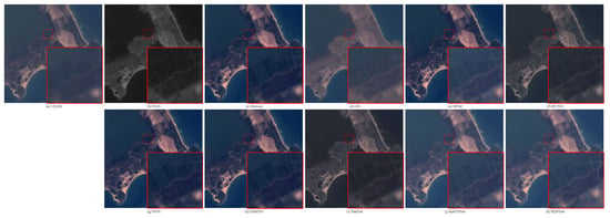
Figure 30.
Subjective comparison between RDFNet and the current mainstream fusion methods for fusion results on the Landsat-7 testing dataset with full resolution. (a) ULMS; (b) PAN; (c) Brovey; (d) GS; (e) SFIM; (f) IFCNN; (g) PNN; (h) DRPNN; (i) PanNet; (j) ResTFNet; (k) RDFNet (ours).
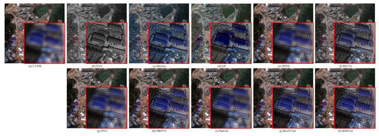
Figure 31.
Subjective comparison between RDFNet and the current mainstream fusion methods for fusion results on the GF-2 testing dataset with full resolution. (a) ULMS; (b) PAN; (c) Brovey; (d) GS; (e) SFIM; (f) IFCNN; (g) PNN; (h) DRPNN; (i) PanNet; (j) ResTFNet; (k) RDFNet (ours).
The objective evaluation indicators for the fusion results of Landsat-8, QuickBird, Landsat-7, and GF-2 with full resolution are shown in Table 2 and Table 3, respectively; the best results are displayed in bold. From the numerical indicators, as shown in Table 2, it can be seen that on the Landsat-8 testing dataset, the value of RDFNet is the best, followed by ResTFNet, DRPNN, PNN, and PanNet. Compared with DRPNN and PNN, the performance of PanNet is worse. Combined with the experimental results of low resolution, the fusion results of PanNet with full resolution show overfitting. From the value of QuickBird testing dataset, as shown in Table 2, it can be observed that although the of RDFNet ranks third (there is little difference with the other two values), the value is the most optimal. In terms of PanNet, because the value of is relatively large, there is serious spectral distortion, so the QNR value is relatively small. However, the values of and are the largest, and the spectral and spatial distortion is serious. The difference of the value of other methods is small. For the digital indexes of the fusion results on the Landsat-7 testing dataset, RDFNet is the best in and , yet, ranked third, with only 0.0018 and 0.0008 difference from first and second, respectively. In terms of GF-2, the index value of RDFNet is the best. From the above analysis, the IFCNN method is not sensitive to remote sensing data and the fusion effect is poor. PanNet shows a serious overfitting phenomenon in our datasets. From an overall point of view, the proposed RDFNet minimizes spectral distortion and spatial distortion, and preserves more spatial details and spectral information.
Table 2.
Quantitative indicators of Landsat-8 and QuickBird fusion results with full resolution.
Table 3.
Quantitative indicators of Landsat-7 and GF-2 fusion results with full resolution.
5. Conclusions
In this paper, we propose a distributed fusion framework based on residual CNN (RCNN), namely, RDFNet, which realizes the data fusion of three channels. It can make the most of the spectral information and spatial information of LRMS and PAN images. The proposed fusion network employs a distributed fusion architecture to make the best of the fusion outcome of the previous step in the fusion channel, so that the subsequent fusion acquires much more spectral and spatial information. Moreover, two feature extraction channels are used to extract the features of MS and PAN images, respectively, using the residual module, and features of different scales are used for the fusion channel. In this way, spectral distortion and spatial information loss are reduced. We employ data from four different satellites to compare the proposed RDFNet, such as Landsat-8, Landsat-7, QuickBird, and GF-2. Comparative experiments are carried out with reduced resolution and full resolution, respectively. The results of the experiment demonstrate that the proposed RDFNet has superior performance in improving spatial resolution and preserving spectral information, and has good robustness and generalization in improving the fusion quality.
Author Contributions
Conceptualization, Y.W.; methodology, Y.W.; software, Y.W.; validation, Y.W.; formal analysis, Y.L.; investigation, M.H. and S.F.; resources, M.H.; data curation, M.H., S.F. and D.W.; writing—original draft preparation, Y.W.; writing—review and editing, Y.W., Y.L. and D.W.; visualization, Y.W.; supervision, M.H. and S.F.; project administration, M.H.; funding acquisition, M.H. All authors have read and agreed to the published version of the manuscript.
Funding
This research was funded by Hainan Provincial Natural Science Foundation of China under Grant 2019CXTD400, and the National Key Research and Development Program of China under Grant 2018YFB1404400.
Institutional Review Board Statement
Not applicable.
Informed Consent Statement
Not applicable.
Data Availability Statement
The data provided in this study can be provided at the request of the corresponding author. The data has not been made public because it is still used for further research in the study field.
Acknowledgments
We greatly thank Sanya Research Center, Institute of Remote Sensing, Chinese Academy of Sciences providing GF-2 data for us. Thank Giuseppe Scarpa for offering codes of PNN in [36]. Thank Wei and Yuan in [39] for sharing DRPNN codes. Thank Yang, J. in [40] for sharing PanNet codes. Thank Liu, X. in [45] for sharing ResTFNet codes.
Conflicts of Interest
The authors declare no conflict of interest.
Abbreviations
The following abbreviations are used in this manuscript:
| MS | Multispectral |
| HRMS | High-resolution multispectral |
| LRMS | Low-resolution multispectral |
| Pan-sharpening | Panchromatic sharpening |
| PAN | Panchromatic |
| CNN | Convolutional neural network |
| RCNN | Residual CNN |
| HRHM | High spatial resolution and high spectral resolution |
| HRHS | High-resolution hyperspectral |
| CS | Component substitution |
| MRA | Multiresolution analysis |
| IHS | Intensity–hue–saturation |
| PCA | Principal component analysis |
| BT | Brovey transform |
| WT | Wavelet transform |
| GS | Gram–Schmidt |
| NSCT | Non-subsampled contourlet transform |
| SFIM | Smoothing filter-based intensity modulation |
| SR | Sparse representation |
| OCDL | Online coupled dictionary learning method |
| DL | Deep learning |
| SRCNN | Super-Resolution Convolutional Neural Network |
| PNN | pan-sharpening by convolutional neural network |
| DRPNN | residual network based panchromatic sharpening |
| HS | hyperspectral |
| GAN | generative adversarial network |
| RED-cGAN | residual encoder–decoder conditional generative adversarial network |
| BN | batch normalization |
| OLI | Operational Land Imager |
| TIRS | Thermal Infrared Sensor |
| CC | correlation coefficient |
| RMSE | Root Mean Square Error |
| SSIM | structural similarity |
| SAM | Spectral angle mapping |
| ERGAS | Erreur Relative Globale Adimensionnelle de Synthése |
| UIQI | universal image quality index |
| QNR | Quality with no reference |
| ULMS | up-sampled low resolution multispectral |
| DLMS | down-sampled low resolution multispectral |
| DULMS | down-sampled and up-sampled low resolution multispectral |
| LPAN | low resolution panchromatic |
| GF-2 | Gaofen-2 |
References
- Ghassemian, H. A review of remote sensing image fusion methods. Inf. Fusion 2016, 32, 75–89. [Google Scholar] [CrossRef]
- Qian, X.; Lin, S.; Cheng, G.; Yao, X.; Ren, H.; Wang, W. Object Detection in Remote Sensing Images Based on Improved Bounding Box Regression and Multi-Level Features Fusion. Remote Sens. 2020, 12, 143. [Google Scholar] [CrossRef] [Green Version]
- Li, S.; Kang, X.; Fang, L.; Hu, J.; Yin, H. Pixel-level image fusion: A survey of the state of the art. Inf. Fusion 2016, 33, 100–112. [Google Scholar] [CrossRef]
- Meng, X.; Shen, H.; Li, H.; Zhang, L.; Fu, R. Review of the Pansharpening Methods for Remote Sensing Images Based on the Idea of Meta-analysis: Practical Discussion and Challenges. Inf. Fusion 2018, 46, 102–113. [Google Scholar] [CrossRef]
- Lu, Z.; Xu, B.; Sun, L.; Zhan, T.; Tang, S. 3D Channel and Spatial Attention Based Multi-Scale Spatial Spectral Residual Network for Hyperspectral Image Classification. IEEE J. Sel. Top. Appl. Earth Obs. Remote Sens. 2020, 13, 4311–4324. [Google Scholar] [CrossRef]
- Carper, W.J.; Lillesand, T.M.; Kiefer, P.W. The use of intensity-hue-saturation transformations for merging SPOT panchromatic and multispectral image data. Photogramm. Eng. Remote Sens. 1990, 56, 459–467. [Google Scholar]
- Tu, T.M.; Su, S.C.; Shyu, H.C.; Huang, P.S. A new look at IHS-like image fusion methods. Inf. Fusion 2001, 2, 177–186. [Google Scholar] [CrossRef]
- Tu, T.M.; Huang, P.S.; Hung, C.L.; Chang, C.P. A Fast Intensity–Hue–Saturation Fusion Technique With Spectral Adjustment for IKONOS Imagery. IEEE Geosci. Remote Sens. Lett. 2004, 1, 309–312. [Google Scholar] [CrossRef]
- Rahmani, S.; Strait, M.; Merkurjev, D.; Moeller, M.; Wittman, T. An Adaptive IHS Pan-Sharpening Method. IEEE Geosci. Remote Sens. Lett. 2010, 7, 746–750. [Google Scholar] [CrossRef] [Green Version]
- Gonzalez-Audicana, M.; Saleta, J.L.; Catalan, R.G.; Garcia, R. Fusion of Multispectral and Panchromatic Images Using Improved IHS and PCA Mergers Based on Wavelet Decomposition. IEEE Trans. Geosci. Remote Sens. 2004, 42, 1291–1299. [Google Scholar] [CrossRef]
- Shahdoosti, H.R. Combining the spectral PCA and spatial PCA fusion methods by an optimal filter. Inf. Fusion 2016, 27, 150–160. [Google Scholar] [CrossRef]
- Shah, V.P.; Younan, N.H.; King, R.L. An Efficient Pan-Sharpening Method via a Combined Adaptive PCA Approach and Contourlets. IEEE Trans. Geosci. Remote Sens. 2008, 46, 1323–1335. [Google Scholar] [CrossRef]
- Li, S.; Yang, B.; Hu, J. Performance comparison of different multi-resolution transforms for image fusion. Inf. Fusion 2011, 12, 74–84. [Google Scholar] [CrossRef]
- Zhou, J.; Civco, D.L.; Silander, J.A. A wavelet transform method to merge Landsat TM and SPOT panchromatic data. Int. J. Remote Sens. 1998, 19, 743–757. [Google Scholar] [CrossRef]
- Nunez, J.; Otazu, X.; Fors, O.; Prades, A.; Pala, V.; Arbiol, R. Multiresolution-based image fusion with additive wavelet decomposition. IEEE Trans. Geosci. Remote Sens. 1999, 37, 1204–1211. [Google Scholar] [CrossRef] [Green Version]
- Upla, K.P.; Joshi, M.V.; Gajjar, P.P. An Edge Preserving Multiresolution Fusion: Use of Contourlet Transform and MRF Prior. IEEE Trans. Geosci. Remote Sens. 2014, 53, 3210–3220. [Google Scholar] [CrossRef]
- Chang, X.; Jiao, L.; Liu, F.; Xin, F. Multicontourlet-Based Adaptive Fusion of Infrared and Visible Remote Sensing Images. IEEE Geosci. Remote Sens. Lett. 2010, 7, 549–553. [Google Scholar] [CrossRef]
- Cunha, D.; Arthur, L.; Zhou, J.; Minh, N. The Nonsubsampled Contourlet Transform: Theory, Design, and Applications. IEEE Trans. Image Process. 2006, 15, 3089–3101. [Google Scholar] [CrossRef] [Green Version]
- Liu, J.G. Smoothing Filter-based Intensity Modulation: A spectral preserve image fusion technique for improving spatial details. Int. J. Remote Sens. 2000, 21, 3461–3472. [Google Scholar] [CrossRef]
- Zhong, S.; Zhang, Y.; Chen, Y.; Wu, D. Combining Component Substitution and Multiresolution Analysis: A Novel Generalized BDSD Pansharpening Algorithm. IEEE J. Sel. Top. Appl. Earth Obs. Remote Sens. 2017, 10, 2867–2875. [Google Scholar] [CrossRef]
- Cheng, M.; Wang, C.; Li, J. Sparse Representation Based Pansharpening Using Trained Dictionary. IEEE Geosci. Remote Sens. Lett. 2014, 11, 293–297. [Google Scholar] [CrossRef]
- Cheng, J.; Liu, H.; Liu, T.; Wang, F.; Li, H. Remote sensing image fusion via wavelet transform and sparse representation. Isprs J. Photogramm. Remote Sens. 2015, 104, 158–173. [Google Scholar] [CrossRef]
- Vicinanza, M.; Restaino, R.; Vivone, G.; Dalla Mura, M.; Chanussot, J. A Pansharpening Method Based on the Sparse Representation of Injected Details. IEEE Geosci. Remote Sens. Lett. 2015, 12, 180–184. [Google Scholar] [CrossRef]
- Burt, P.J.; Adelson, E.H. The Laplacian Pyramid as a Compact Image Code. Read Comput. Vis. 1987, 31, 671–679. [Google Scholar]
- Vivone, G.; Marano, S.; Chanussot, J. Pansharpening: Context-Based Generalized Laplacian Pyramids by Robust Regression. IEEE Trans. Geosci. Remote Sens. 2020, 58, 6152–6167. [Google Scholar] [CrossRef]
- Ghahremani, M.; Ghassemian, H. Remote-sensing image fusion based on curvelets and ICA. Int. J. Remote Sens. 2015, 36, 4131–4143. [Google Scholar] [CrossRef]
- Ji, X.; Zhang, G. Image fusion method of SAR and infrared image based on Curvelet transform with adaptive weighting. Multimed. Tools Appl. 2015, 76, 17633–17649. [Google Scholar] [CrossRef]
- Wei, Q.; Dobigeon, N.; Tourneret, J.Y. Bayesian Fusion of Multi-Band Images. IEEE J. Sel. Top. Signal Process. 2015, 9, 1117–1127. [Google Scholar] [CrossRef] [Green Version]
- Guo, M.; Zhang, H.; Li, J.; Zhang, L.; Shen, H. An Online Coupled Dictionary Learning Approach for Remote Sensing Image Fusion. IEEE J. Sel. Top. Appl. Earth Obs. Remote Sens. 2014, 7, 1284–1294. [Google Scholar] [CrossRef]
- Huang, B.; Song, H.; Cui, H.; Peng, J. Spatial and Spectral Image Fusion Using Sparse Matrix Factorization. IEEE Trans. Geosci. Remote Sens. 2013, 52, 1693–1704. [Google Scholar] [CrossRef]
- Sun, L.; He, C.; Zheng, Y.; Tang, S. SLRL4D: Joint Restoration of Subspace Low-Rank Learning and Non-Local 4-D Transform Filtering for Hyperspectral Image. Remote Sens. 2020, 12, 2979. [Google Scholar] [CrossRef]
- Joshi, M.V.; Chaudhuri, S.; Panuganti, R. A learning-based method for image super-resolution from zoomed observations. IEEE Trans. Syst. Man Cybern. Part B 2005, 35, 527–537. [Google Scholar] [CrossRef]
- Dong, C.; Loy, C.C.; He, K.; Tang, X. Image Super-Resolution Using Deep Convolutional Networks. IEEE Trans. Pattern Anal. Mach. Intell. 2016, 38, 295–307. [Google Scholar] [CrossRef] [Green Version]
- Dong, W.; Fu, F.; Shi, G.; Cao, X.; Wu, J.; Li, G.; Li, X. Hyperspectral Image Super-Resolution via Non-Negative Structured Sparse Representation. IEEE Trans. Image Process. 2016, 25, 2337–2352. [Google Scholar] [CrossRef]
- Huang, W.; Xiao, L.; Liu, H.; Wei, Z.; Tang, S. A New Pan-Sharpening Method With Deep Neural Networks. IEEE Geosci. Remote Sens. Lett. 2015, 12, 1037–1041. [Google Scholar] [CrossRef]
- Giuseppe, M.; Davide, C.; Luisa, V.; Giuseppe, S. Pansharpening by Convolutional Neural Networks. Remote Sens. 2016, 8, 594. [Google Scholar]
- Azarang, A.; Ghassemian, H. A new pansharpening method using multi resolution analysis framework and deep neural networks. In Proceedings of the International Conference on Pattern Recognition and Image Analysis, Shahrekord, Iran, 19–20 April 2017; pp. 1–5. [Google Scholar]
- Rao, Y.; He, L.; Zhu, J. A residual convolutional neural network for pan-shaprening. In Proceedings of the International Workshop on Remote Sensing with Intelligent Processing (RSIP), Shanghai, China, 19–21 May 2017; pp. 1–4. [Google Scholar]
- Wei, Y.; Yuan, Q.; Shen, H.; Zhang, L. Boosting the Accuracy of Multispectral Image Pansharpening by Learning a Deep Residual Network. IEEE Geosci. Remote Sens. Lett. 2017, 14, 1795–1799. [Google Scholar] [CrossRef] [Green Version]
- Yang, J.; Fu, X.; Hu, Y.; Huang, Y.; Ding, X.; Paisley, J. PanNet: A Deep Network Architecture for Pan-Sharpening. In Proceedings of the 2017 IEEE International Conference on Computer Vision (ICCV), Venice, Italy, 22–29 October 2017; pp. 1753–1761. [Google Scholar]
- Yuan, Q.; Wei, Y.; Meng, X.; Shen, H.; Zhang, L. A Multi-Scale and Multi-Depth Convolutional Neural Network for Remote Sensing Imagery Pan-Sharpening. IEEE J. Sel. Top. Appl. Earth Obs. Remote Sens. 2018, 11, 978–989. [Google Scholar] [CrossRef] [Green Version]
- Palsson, F.; Sveinsson, J.R.; Ulfarsson, M.O. Multispectral and Hyperspectral Image Fusion Using a 3-D-Convolutional Neural Network. IEEE Geosci. Remote Sens. Lett. 2017, 14, 639–643. [Google Scholar] [CrossRef]
- Shao, Z.; Cai, J. Remote Sensing Image Fusion With Deep Convolutional Neural Network. IEEE J. Sel. Top. Appl. Earth Obs. Remote Sens. 2018, 11, 1656–1669. [Google Scholar] [CrossRef]
- Scarpa, G.; Vitale, S.; Cozzolino, D. Target-Adaptive CNN-Based Pansharpening. IEEE Trans. Geosci. Remote Sens. 2018, 56, 5443–5457. [Google Scholar] [CrossRef] [Green Version]
- Liu, X.; Liu, Q.; Wang, Y. Remote sensing image fusion based on two-stream fusion network. Inf. Fusion 2020, 55, 1–15. [Google Scholar] [CrossRef] [Green Version]
- Liu, X.; Wang, Y.; Liu, Q. Psgan: A Generative Adversarial Network for Remote Sensing Image Pan-Sharpening. In Proceedings of the IEEE International Conference on Image Processing, Athens, Greece, 7–10 October 2018; pp. 873–877. [Google Scholar]
- Shao, Z.; Lu, Z.; Ran, M.; Fang, L.; Zhou, J.; Zhang, Y. Residual Encoder-Decoder Conditional Generative Adversarial Network for Pansharpening. IEEE Geosci. Remote Sens. Lett. 2019, 17, 1573–1577. [Google Scholar] [CrossRef]
- Ma, J.; Yu, W.; Chen, C.; Liang, P.; Guo, X.; Jiang, J. Pan-GAN: An unsupervised pan-sharpening method for remote sensing image fusion. Inf. Fusion 2020, 62, 110–120. [Google Scholar] [CrossRef]
- Mnks, U.; Trsek, H.; Dürkop, L.; Genei, V.; Lohweg, V. Towards distributed intelligent sensor and information fusion. Mechatronics 2016, 34, 63–71. [Google Scholar] [CrossRef]
- Liggins, M.E.; Hall, D.L.; James, L. Handbook of Multisensor Data Fusion: Theory and Practice; CRC Press: Boca Raton, FL, USA, 2008; pp. 165–176. [Google Scholar]
- Liggins, M.E.; Chong, C.Y.; Kadar, I.; Alford, M.; Vannicola, V.; Thomopoulos, S. Distributed fusion architectures and algorithms for target tracking. Proc. IEEE 1997, 85, 95–107. [Google Scholar] [CrossRef] [Green Version]
- He, K.; Zhang, X.; Ren, S.; Sun, J. Deep Residual Learning for Image Recognition. In Proceedings of the IEEE Conference on Computer Vision and Pattern Recognition, Las Vegas, NV, USA, 27–30 June 2016; pp. 770–778. [Google Scholar]
- He, K.; Zhang, X.; Ren, S.; Sun, J. Identity Mappings in Deep Residual Networks. In Proceedings of the European Conference on Computer Vision, Amsterdam, The Netherlands, 8–16 October 2016; pp. 630–645. [Google Scholar]
- Vivone, G.; Alparone, L.; Chanussot, J.; Mura, M.; Garzelli, A.; Licciardi, G.A.; Restaino, R.; Wald, L. A Critical Comparison Among Pansharpening Algorithms. IEEE Trans. Geosci. Remote Sens. 2015, 53, 2565–2586. [Google Scholar] [CrossRef]
- Aiazzi, B.; Alparone, L.; Baronti, S.; Garzelli, A.; Selva, M. MTF-tailored Multiscale Fusion of High-resolution MS and Pan Imagery. Photogramm. Eng. Remote Sens. 2006, 72, 591–596. [Google Scholar] [CrossRef]
- Wald, L.; Ranchin, T.; Mangolini, M. Fusion of satellite images of different spatial resolutions: Assessing the quality of resulting images. Photogramm. Eng. Remote Sens. 1997, 63, 691–699. [Google Scholar]
- Kingma, D.; Ba, J. Adam: A Method for Stochastic Optimization. arXiv 2014, arXiv:1412.6980. [Google Scholar]
- Aiazzi, B.; Baronti, S.; Selva, M.; Alparone, L. Bi-cubic interpolation for shift-free pan-sharpening. Isprs J. Photogramm. Remote Sens. 2013, 86, 65–76. [Google Scholar] [CrossRef]
- Zhu, X.X.; Bamler, R. A Sparse Image Fusion Algorithm with Application to Pan-Sharpening. IEEE Trans. Geosci. Remote Sens. 2013, 51, 2827–2836. [Google Scholar] [CrossRef]
- Wang, Z.; Bovik, A.C.; Sheikh, H.R.; Simoncelli, E.P. Image quality assessment: From error visibility to structural similarity. IEEE Trans. Image Process. 2004, 13, 600–612. [Google Scholar] [CrossRef] [PubMed] [Green Version]
- Yuhas, R.H.; Goetz, A.F.H.; Boardman, J.W. Discrimination among semi-arid landscape endmembers using the Spectral Angle Mapper (SAM) algorithm. In Proceedings of the Summaries of the Third Annual JPL Airborne Geoscience Workshop, Pasadena, CA, USA, 1–5 June 1992; pp. 147–149. [Google Scholar]
- Wang, Z.; Bovik, A.C. A universal image quality index. IEEE Signal Process. Lett. 2002, 9, 81–84. [Google Scholar] [CrossRef]
- Alparone, L.; Aiazzi, B.; Baronti, S.; Garzelli, A.; Nencini, F.; Selva, M. Multispectral and Panchromatic Data Fusion Assessment Without Reference. Photogramm. Eng. Remote Sens. 2008, 74, 193–200. [Google Scholar] [CrossRef] [Green Version]
- Zhang, Y.; Liu, Y.; Sun, P.; Yan, H.; Zhao, X.; Zhang, L. IFCNN: A general image fusion framework based on convolutional neural network. Inf. Fusion 2020, 54, 99–118. [Google Scholar] [CrossRef]
- Qu, Y.; Baghbaderani, R.K.; Qi, H.; Kwan, C. Unsupervised Pansharpening Based on Self-Attention Mechanism. IEEE Trans. Geosci. Remote Sens. 2020, 59, 3192–3208. [Google Scholar] [CrossRef]
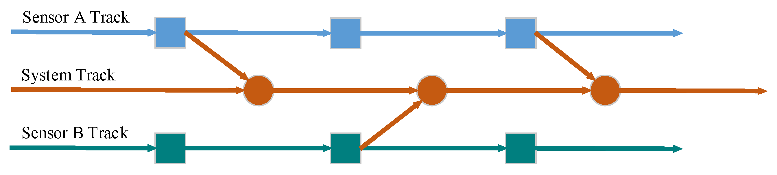
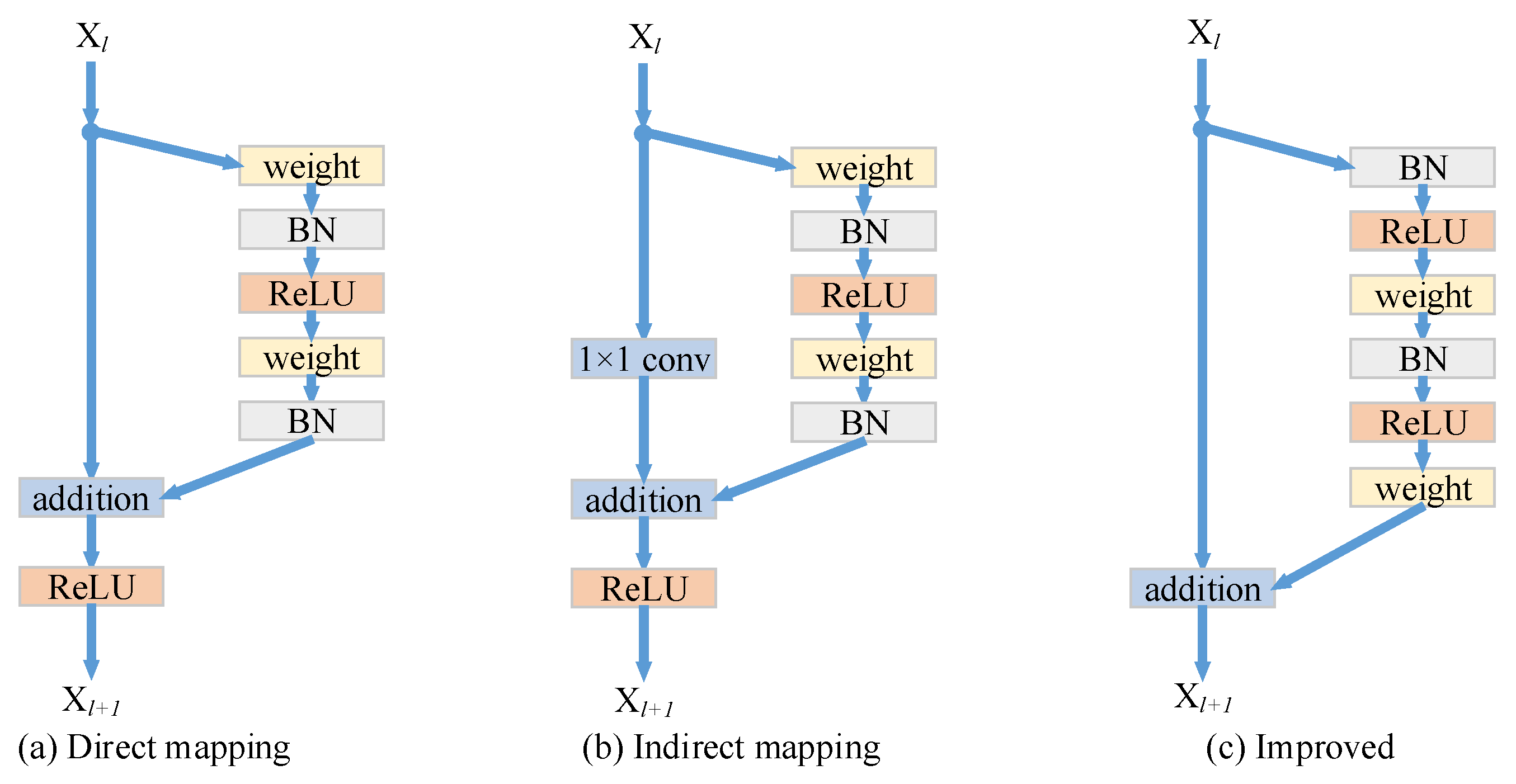
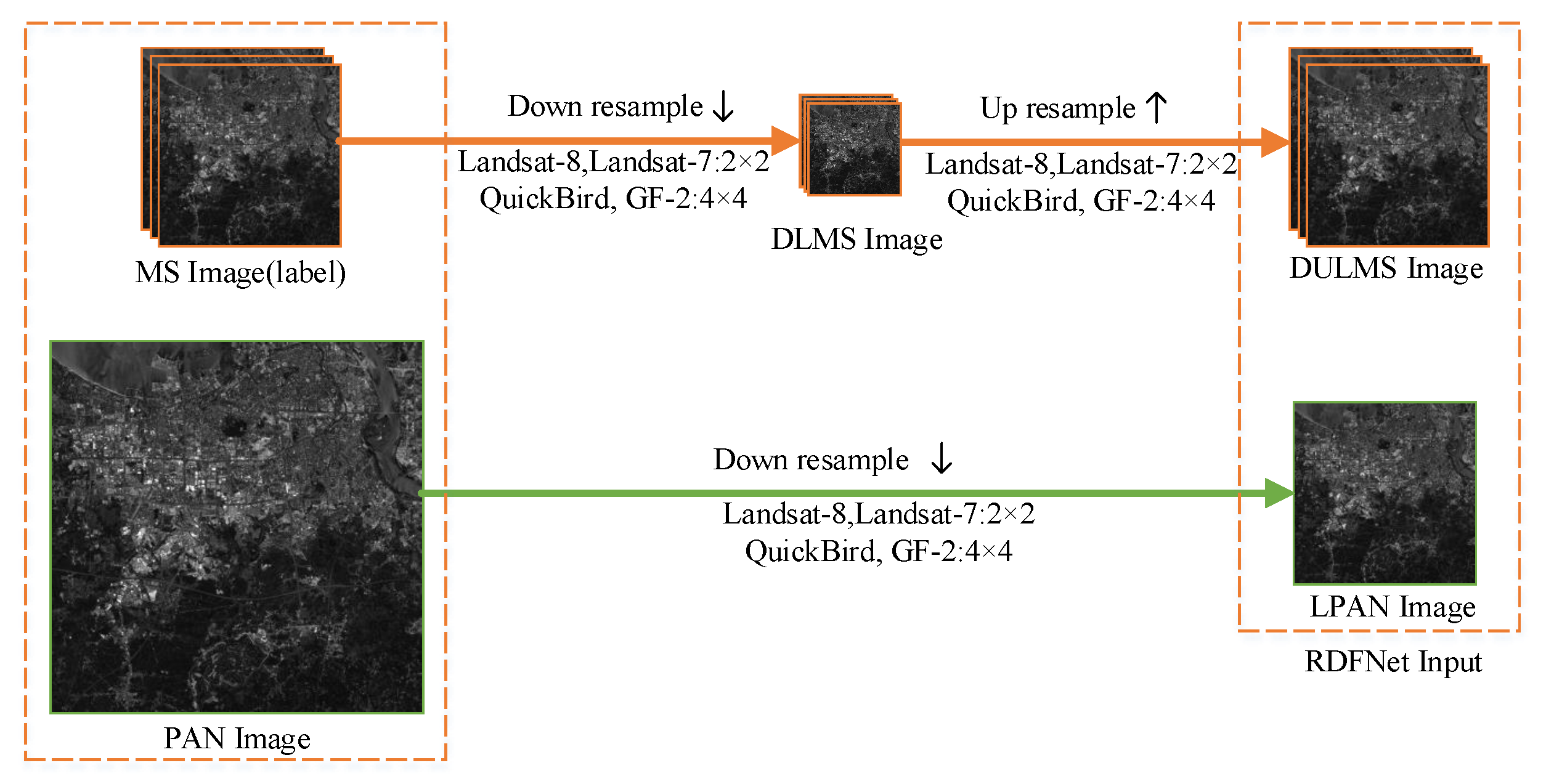
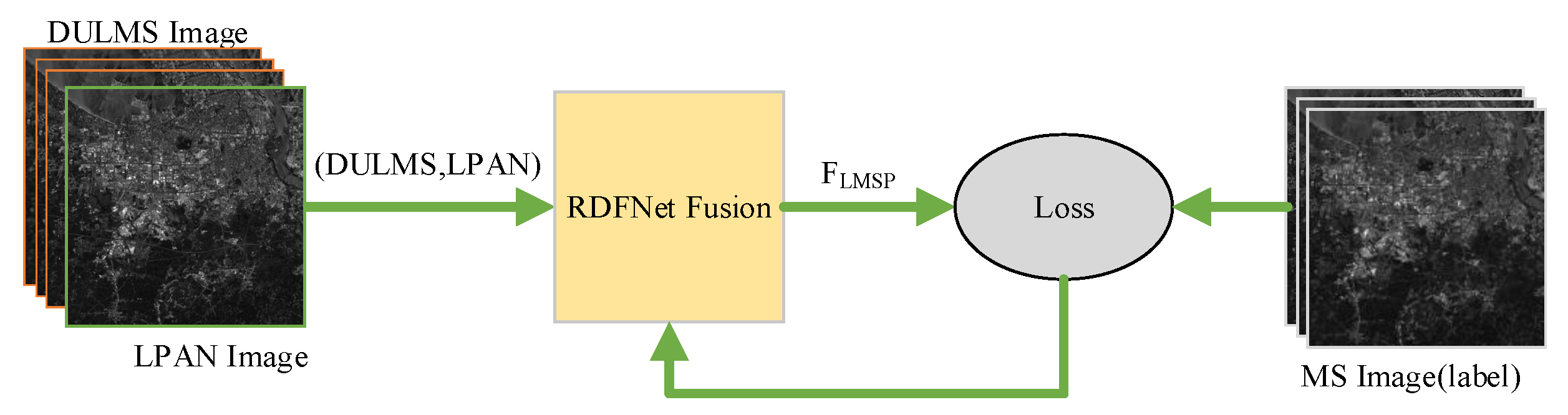
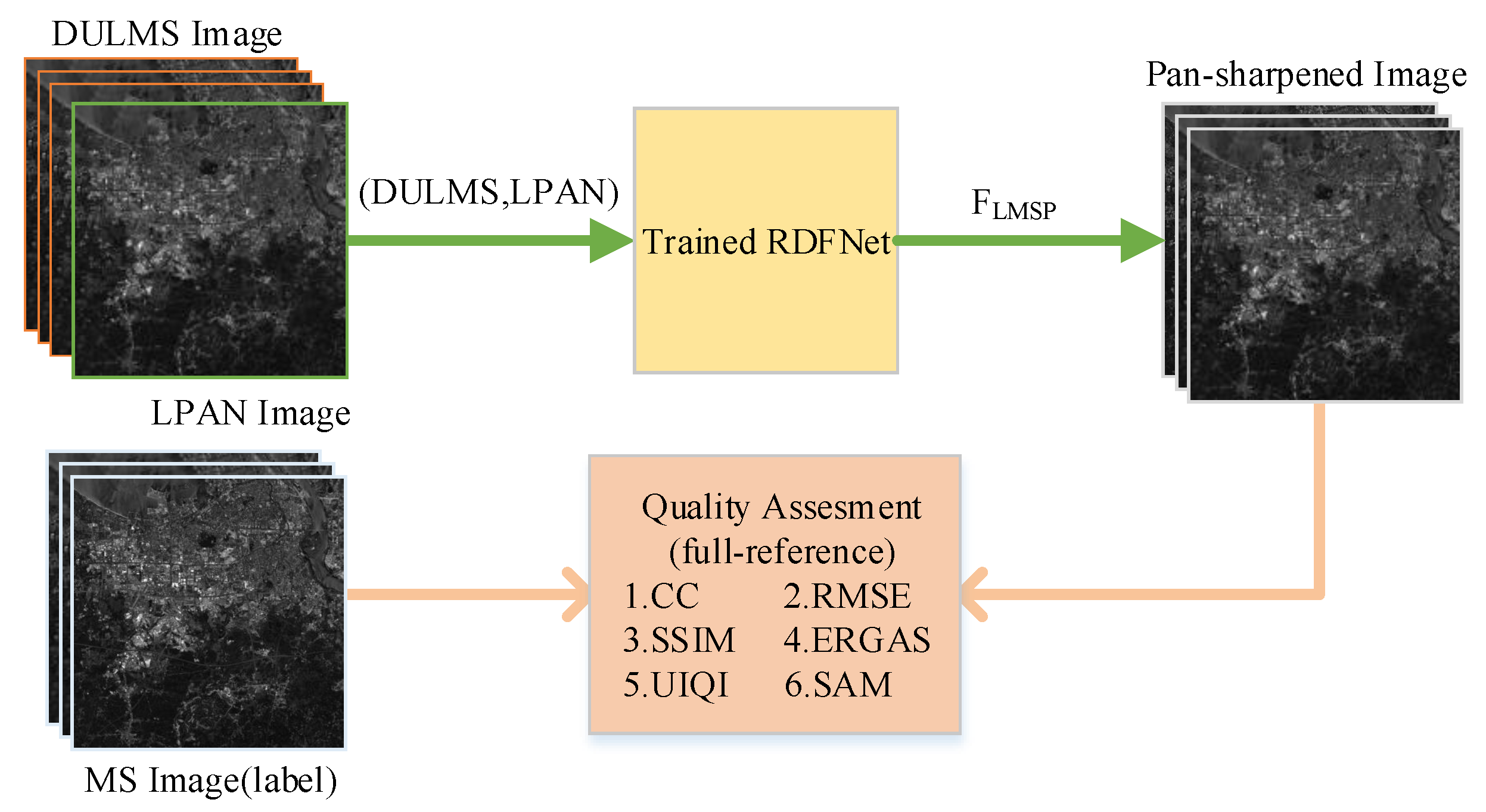
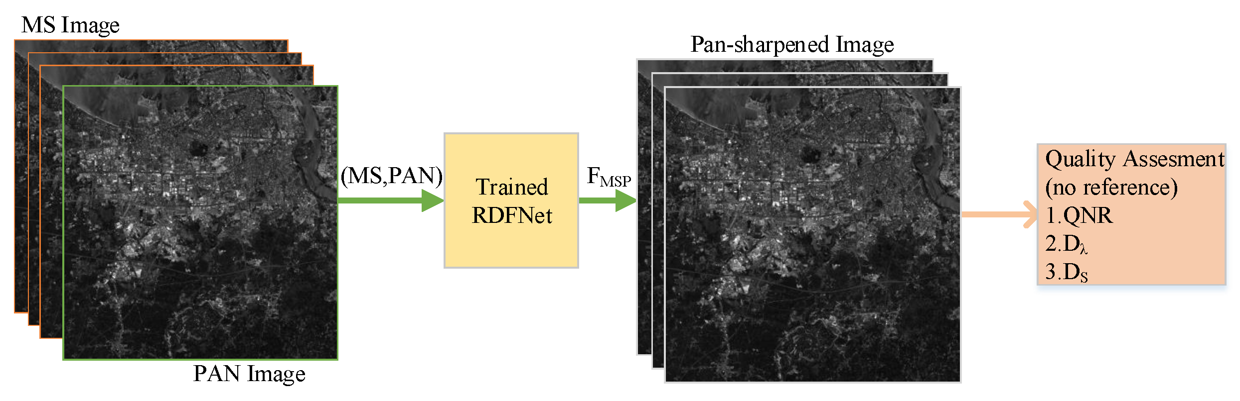
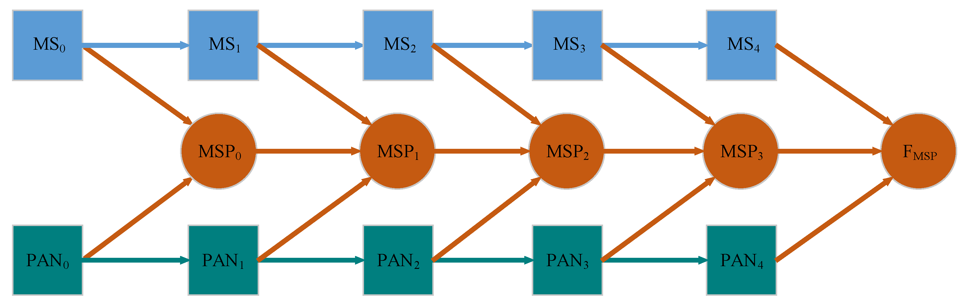

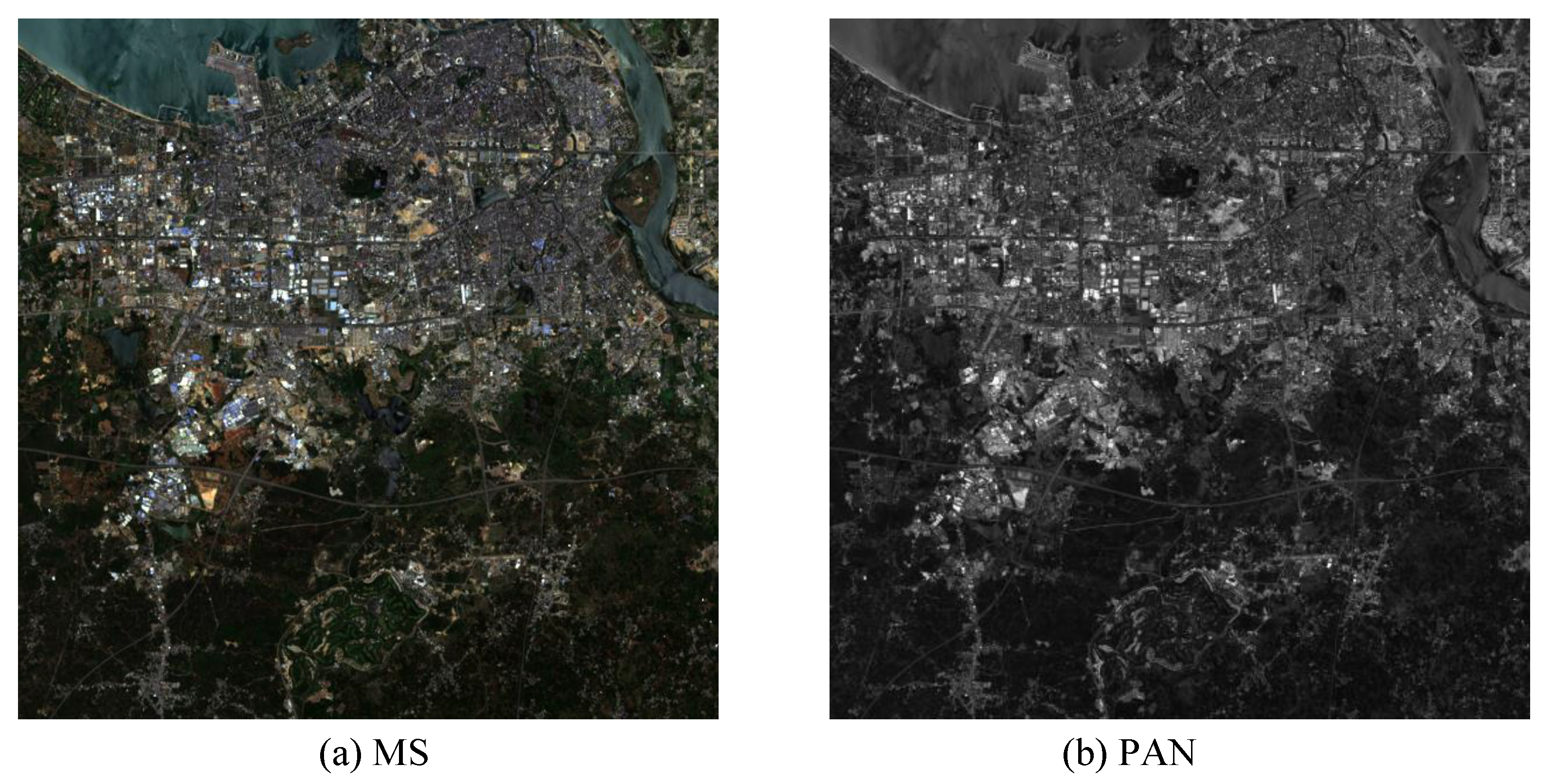
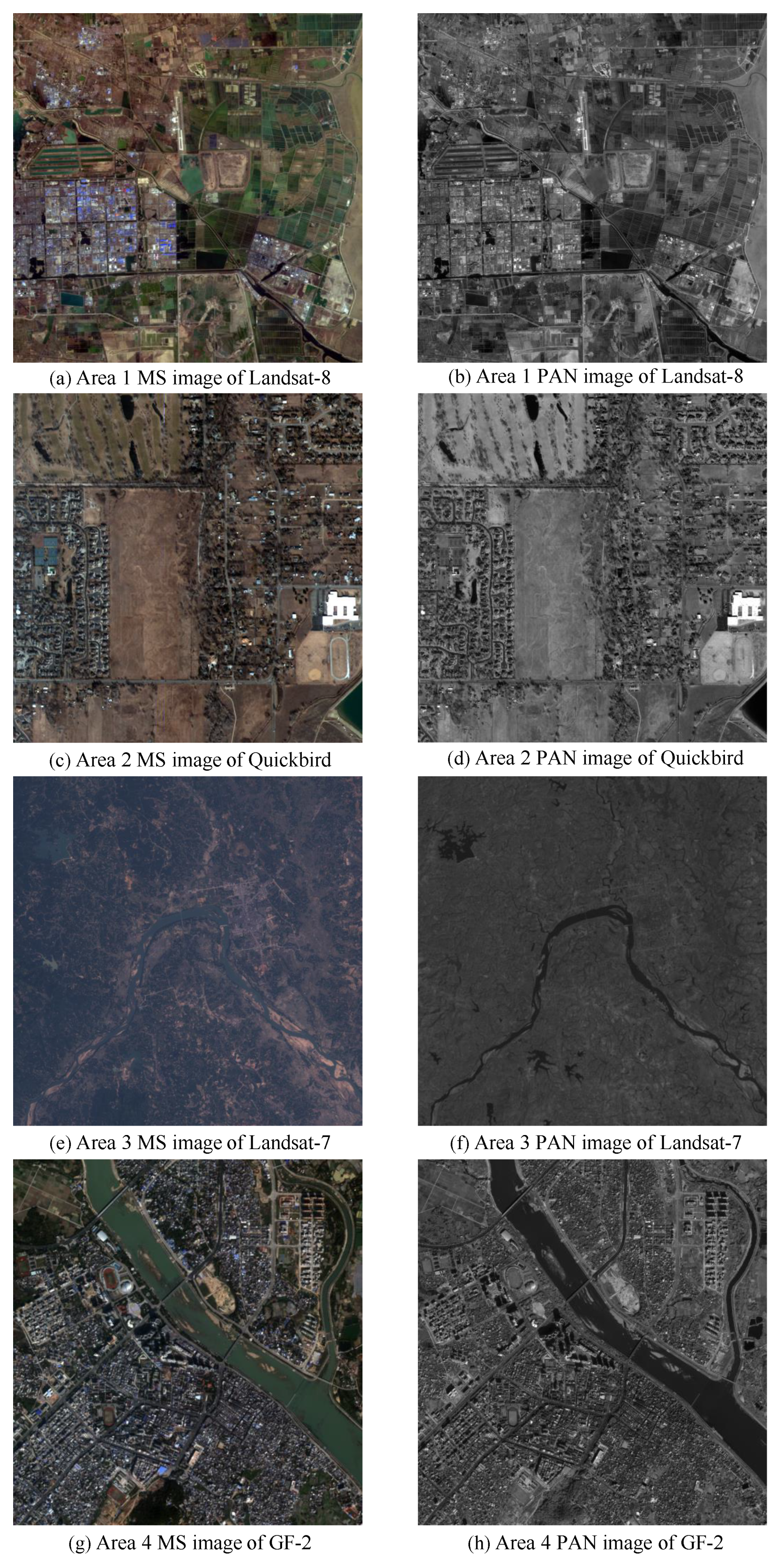
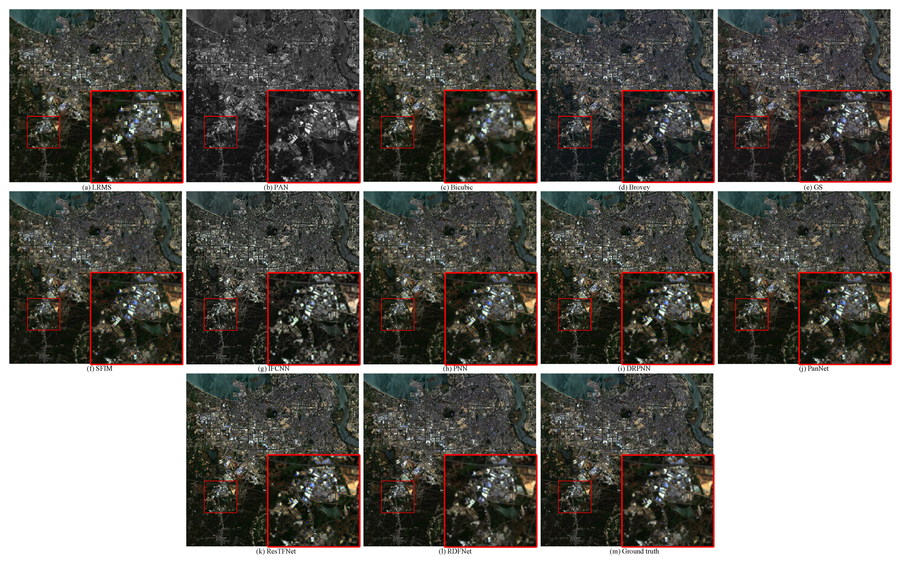
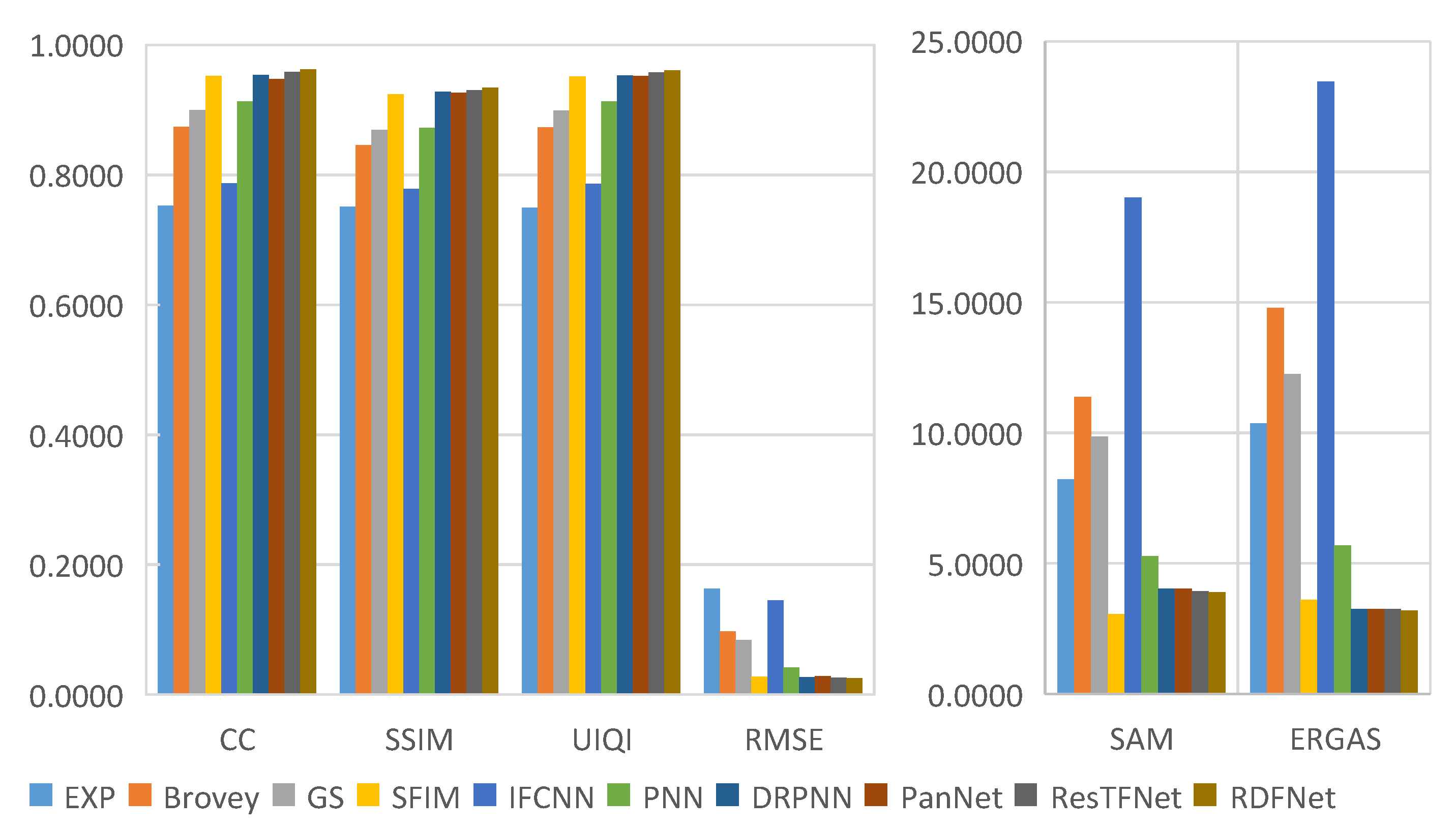
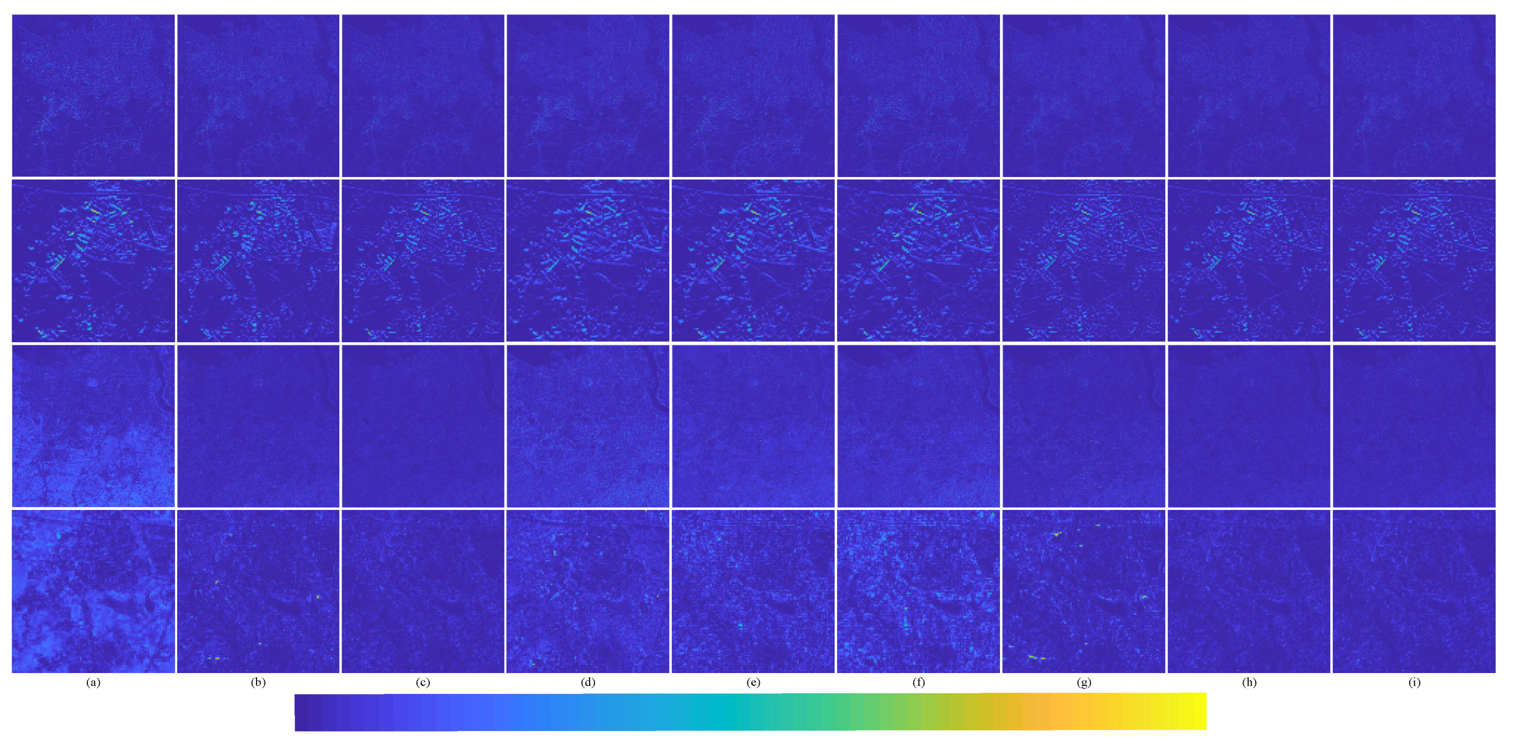
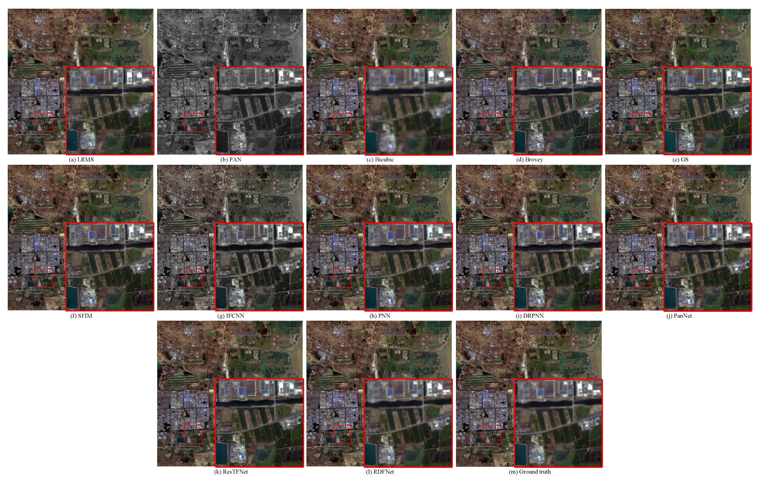
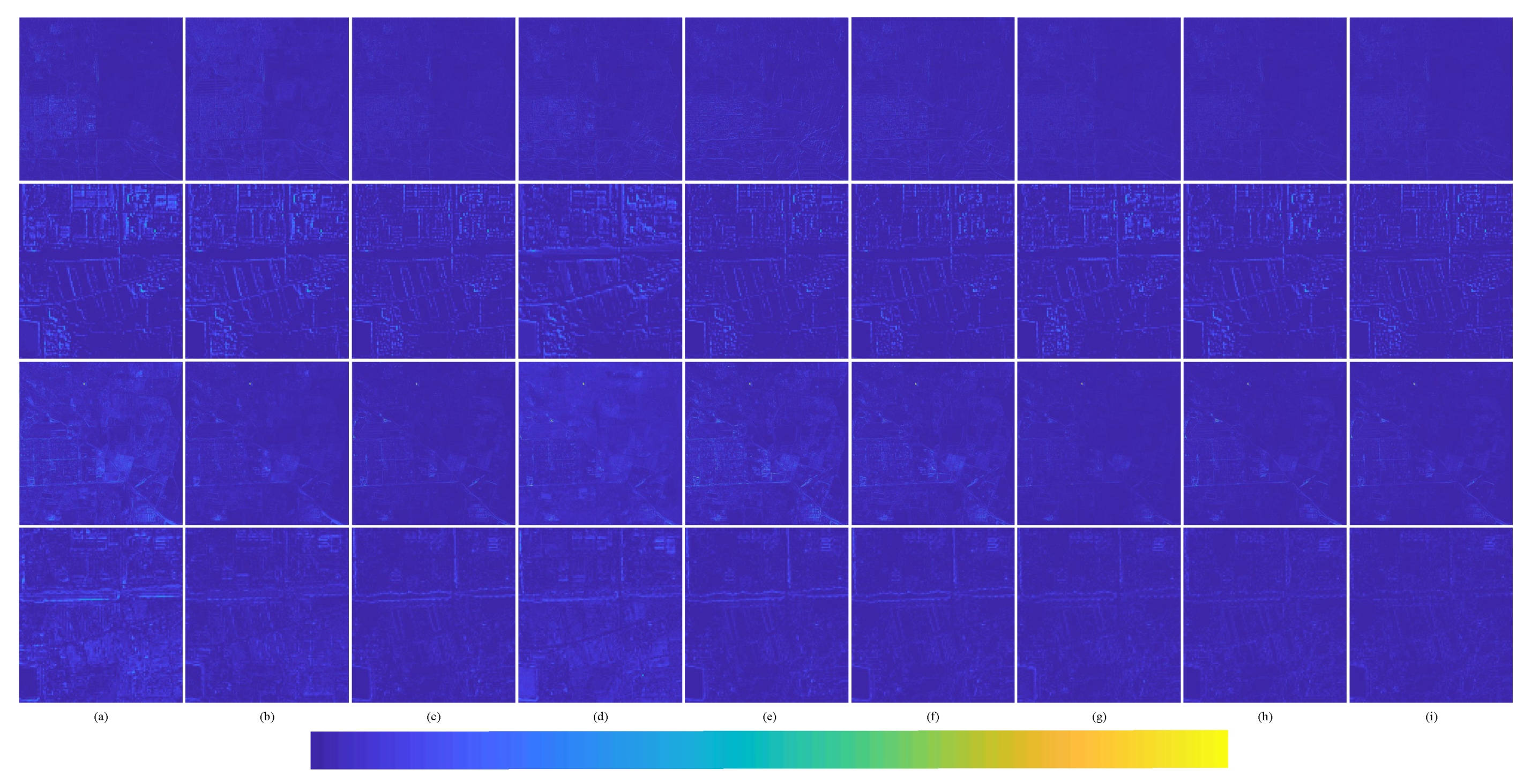
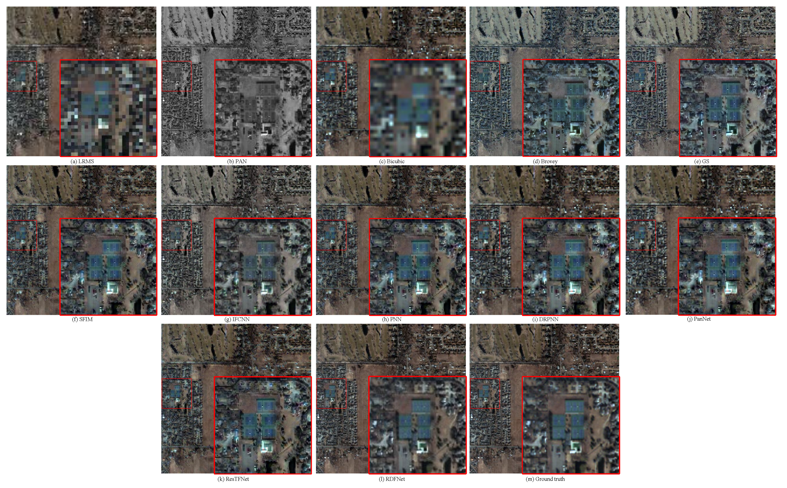
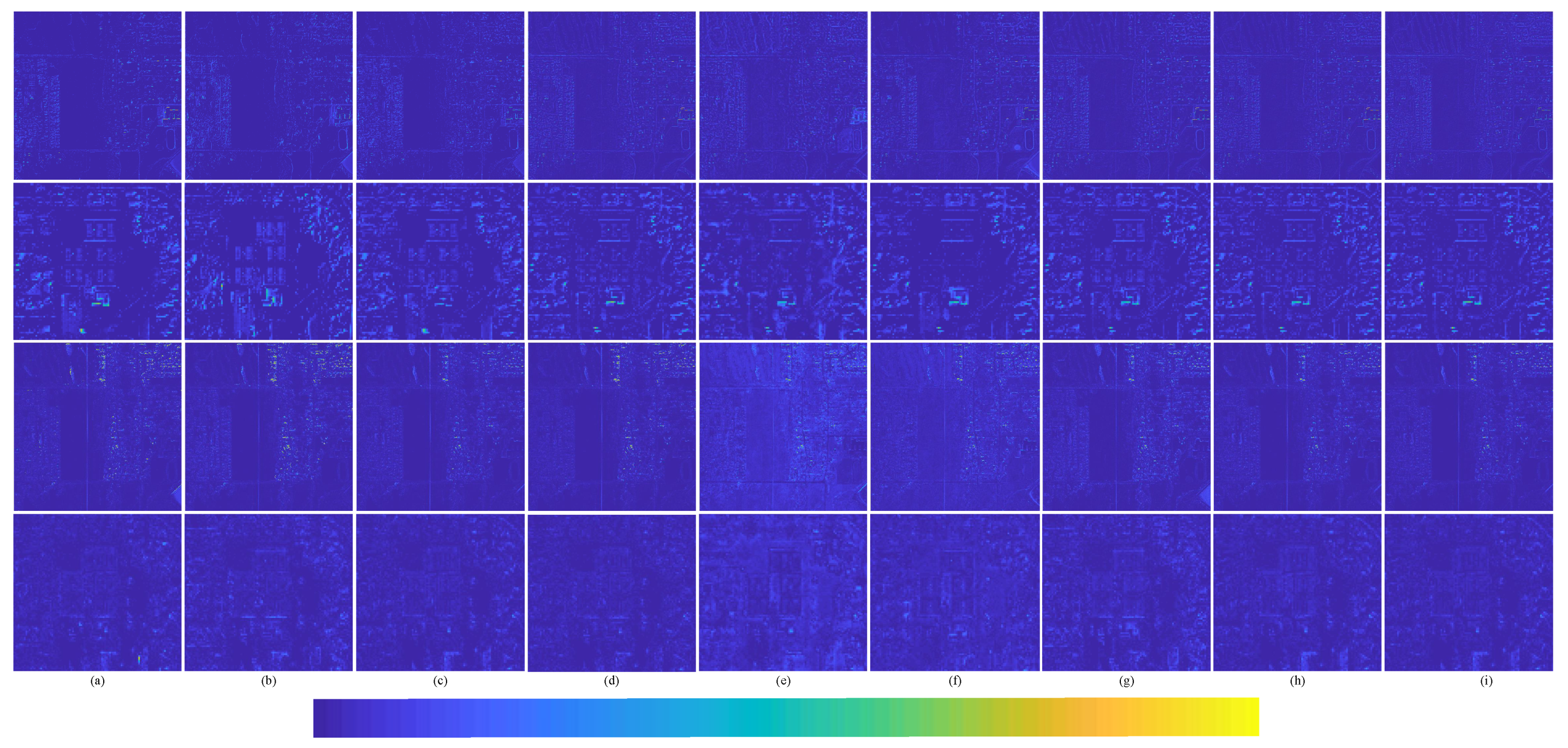
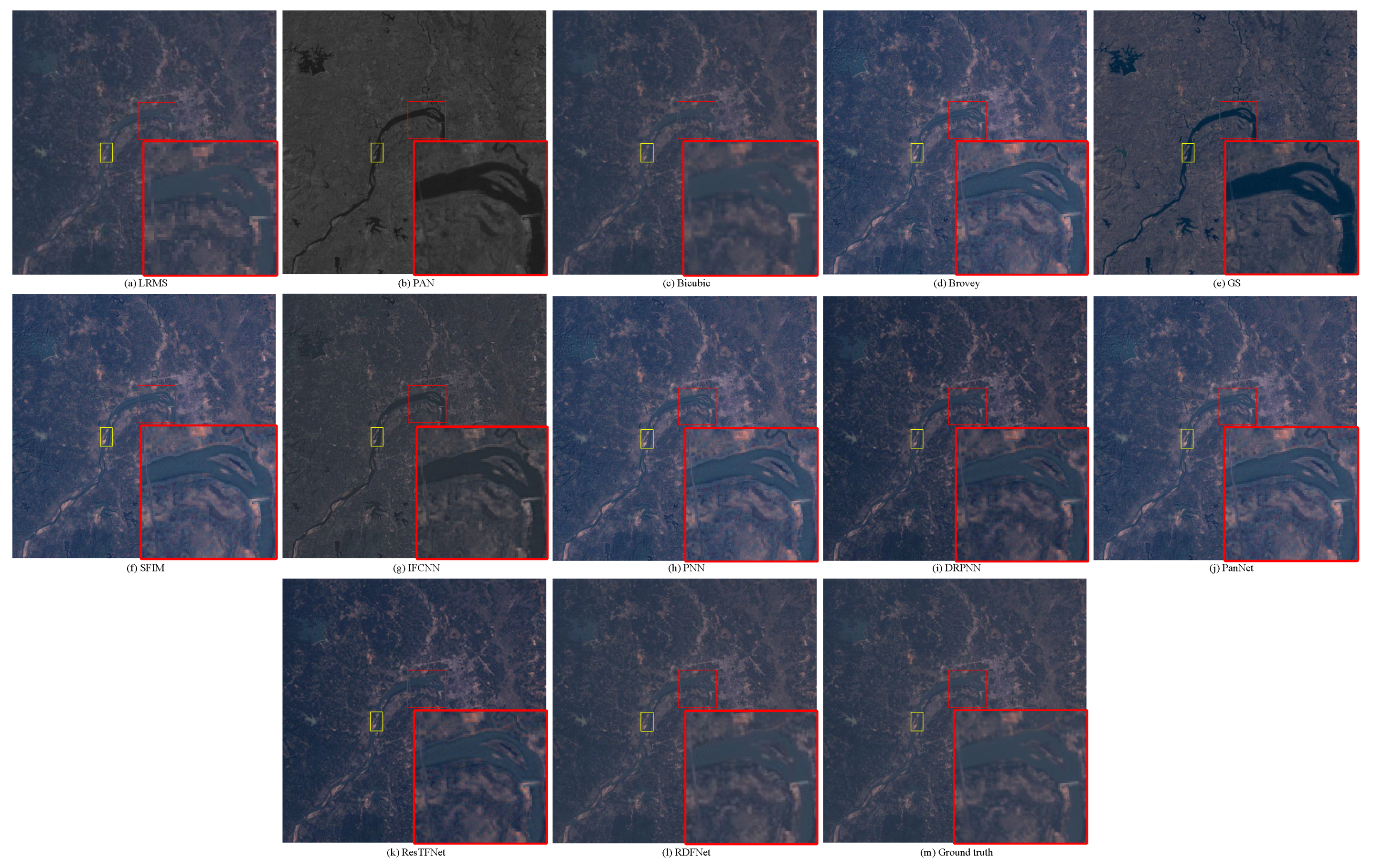
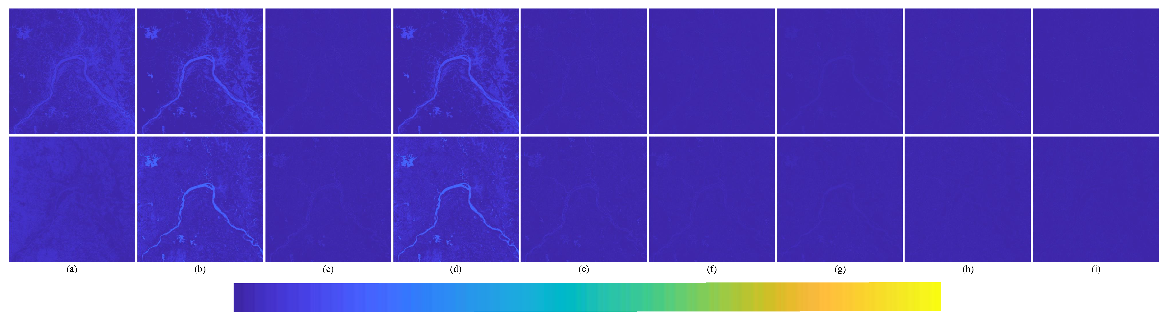
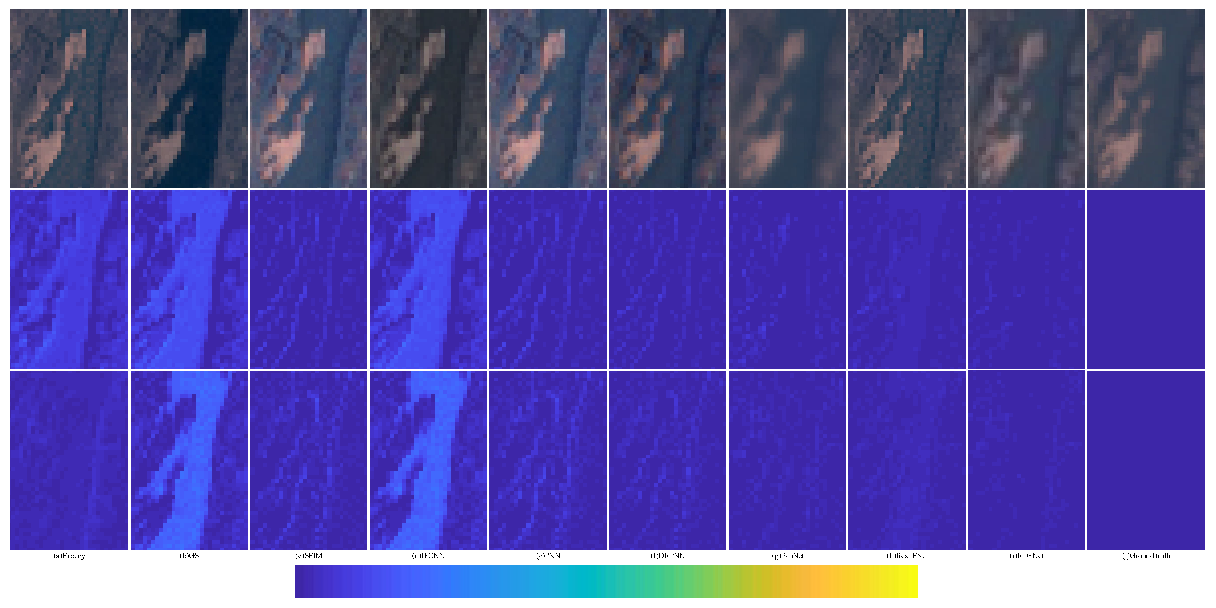
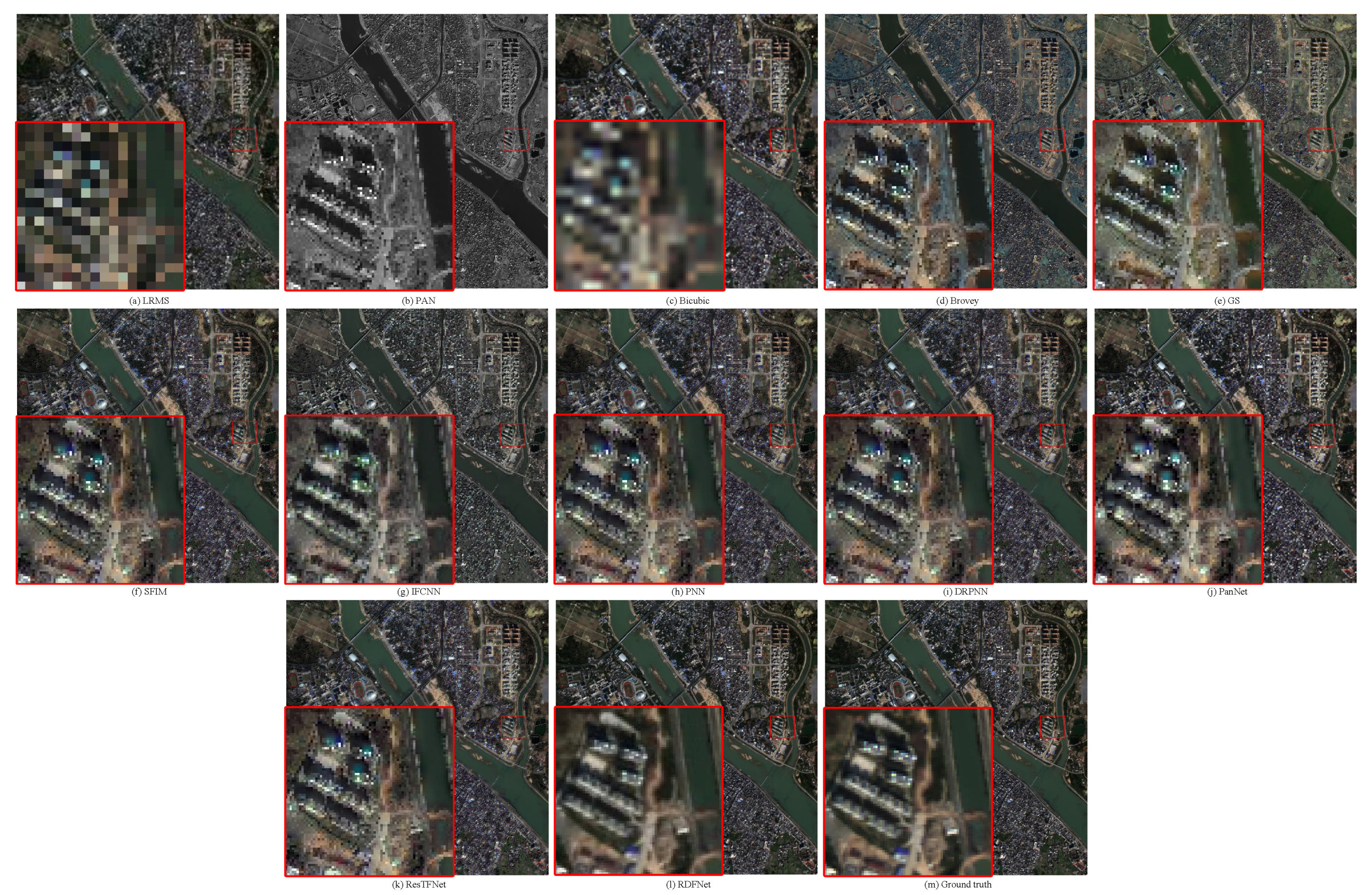
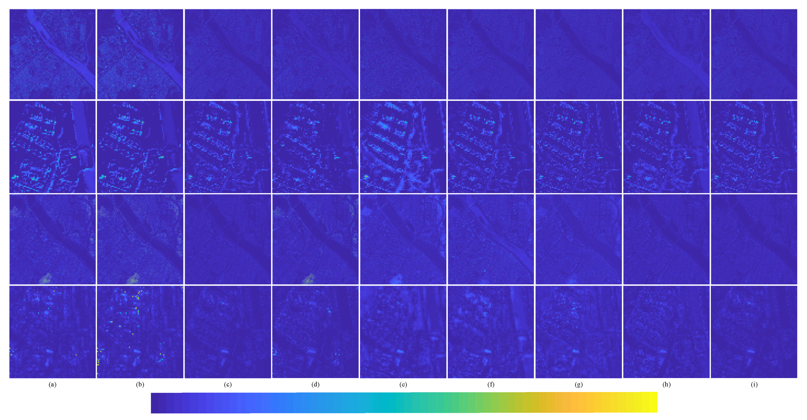
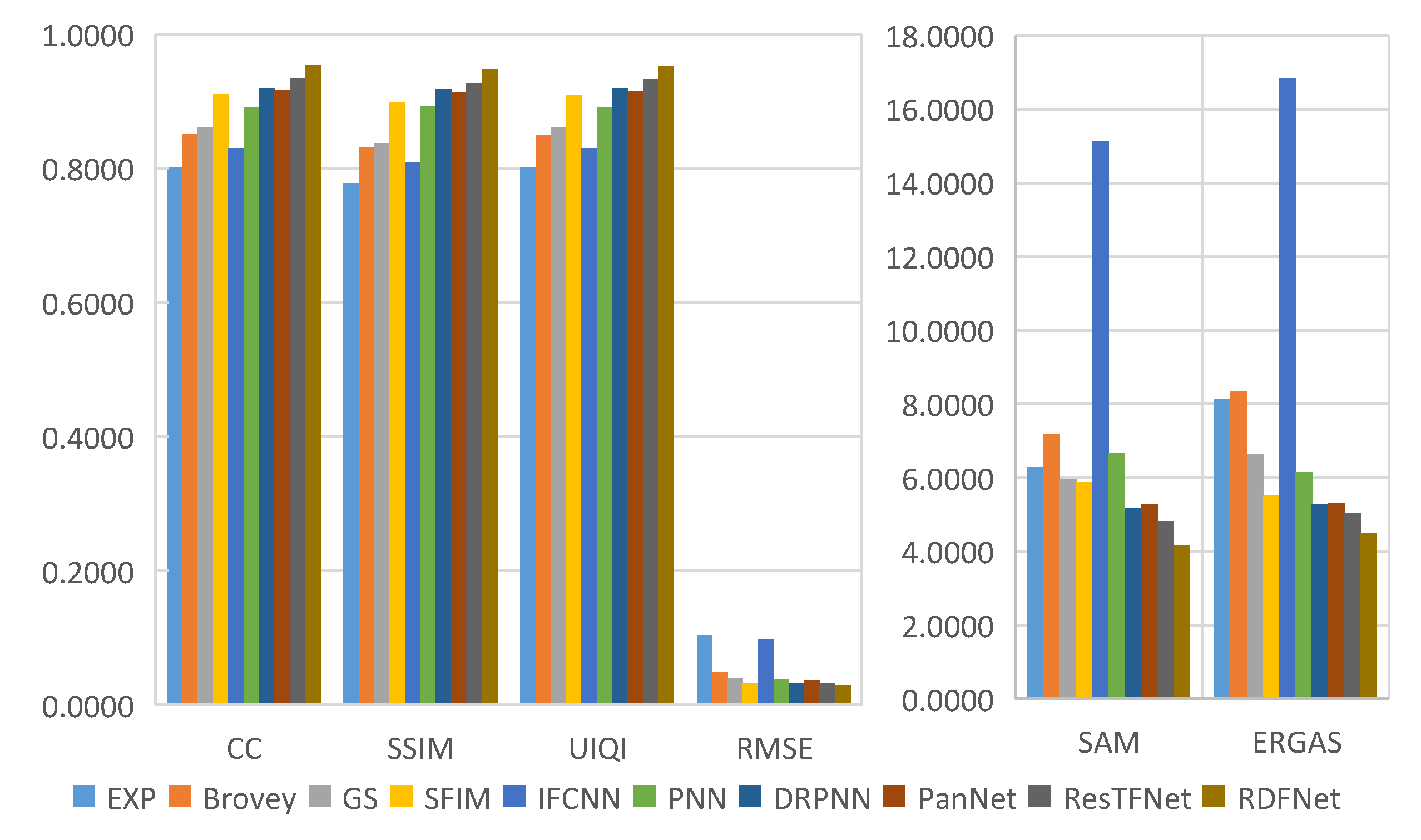
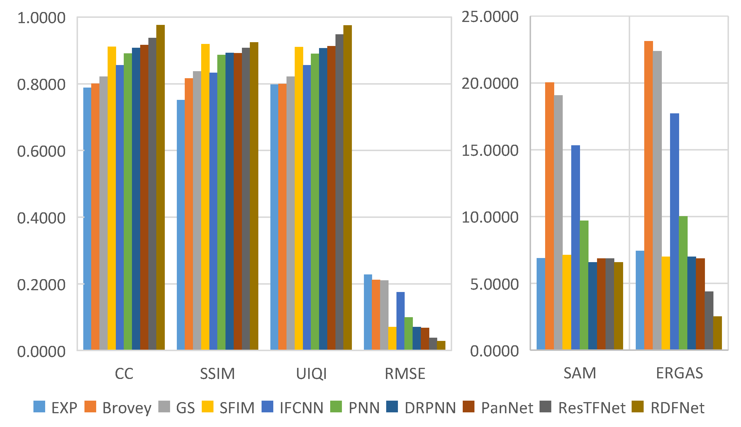
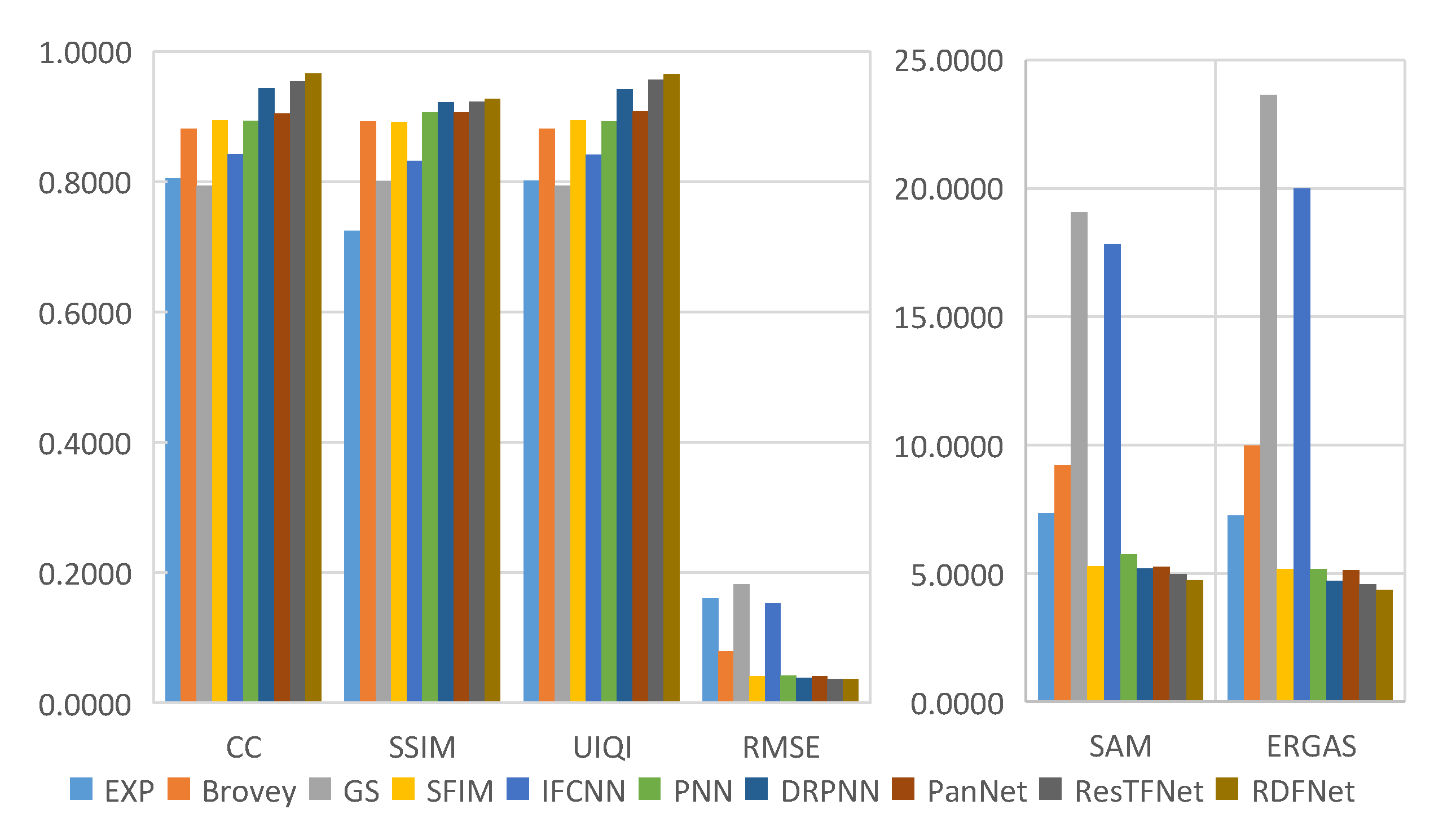
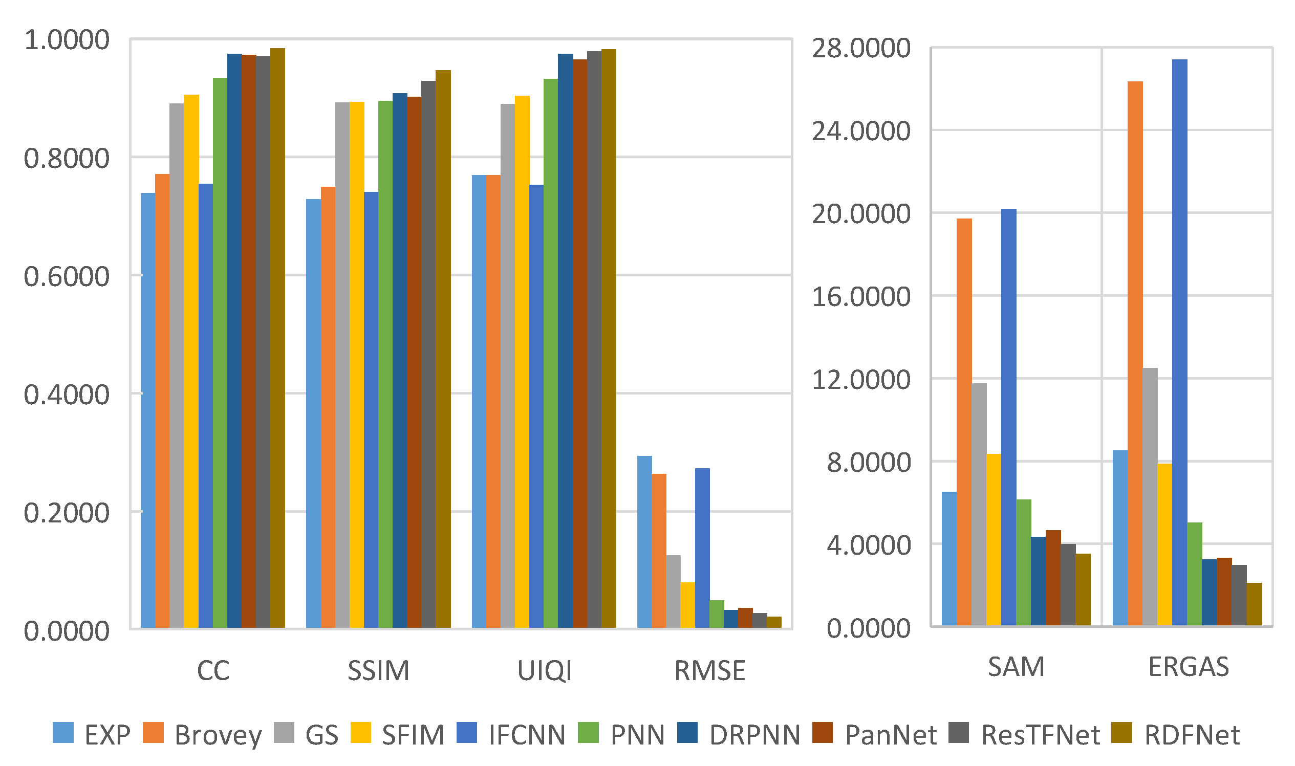
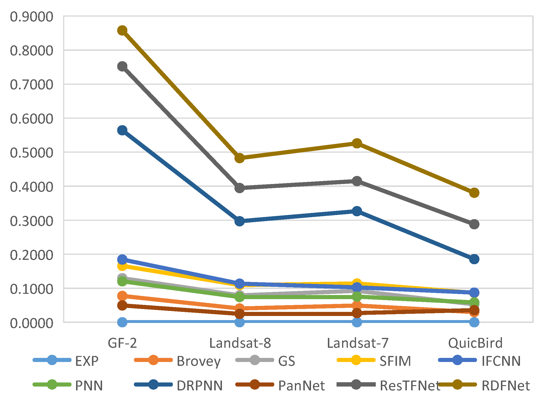
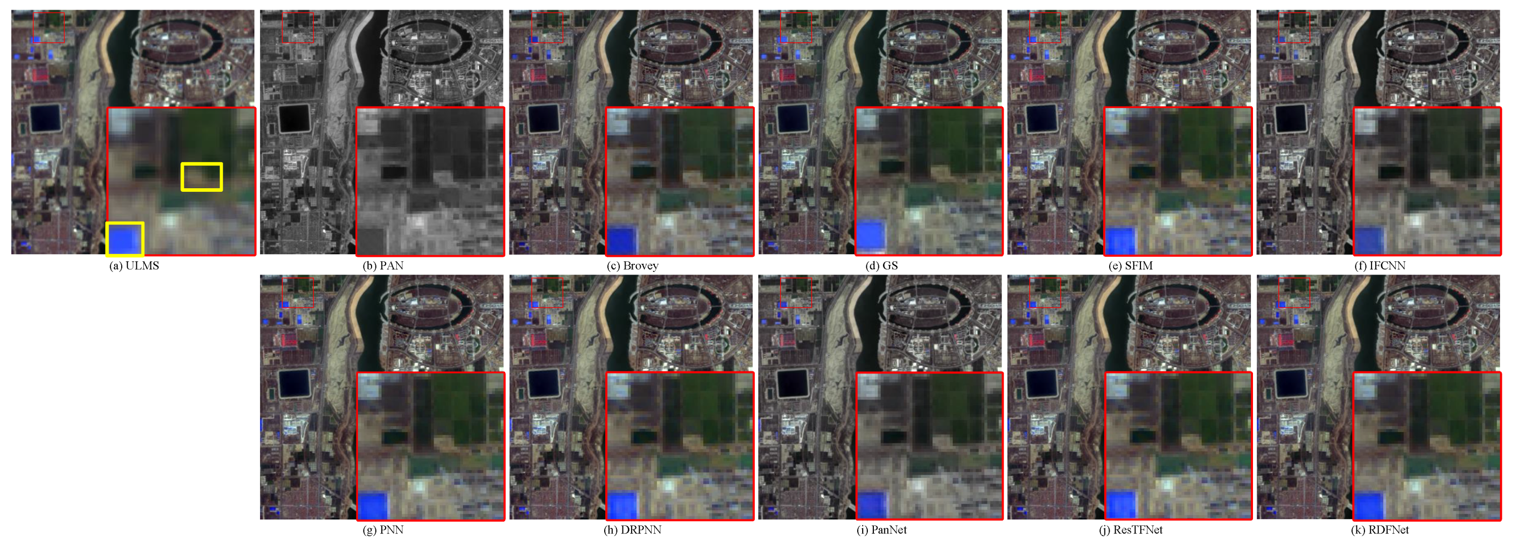
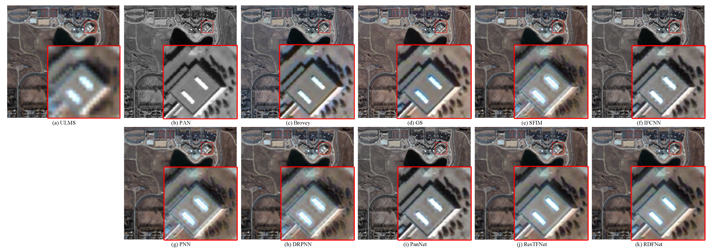


Publisher’s Note: MDPI stays neutral with regard to jurisdictional claims in published maps and institutional affiliations. |
© 2021 by the authors. Licensee MDPI, Basel, Switzerland. This article is an open access article distributed under the terms and conditions of the Creative Commons Attribution (CC BY) license (https://creativecommons.org/licenses/by/4.0/).