
A Colourimetric Approach to Ecological Remote Sensing: Case Study for the Rainforests of South-Eastern Australia


Abstract
:
1. Introduction
1.1. Rationale for a Colourimetric Approach
1.1.1. Colourimetry and Interpretation
1.1.2. Scalability
1.1.3. Reducing Sampling Cost with Satellite Imagery Interpretation
1.2. Colourimetric Ontologies and Multidimensional Colour Blending
1.3. Simplicity and Transparency through One-Class, One-Index Density Slicing
2. Case Study: Rainforests of South-Eastern Australia
Existing Approaches to Rainforest Mapping and the Need for Detail and Automation
3. Methods
3.1. Study Area and Knowledge Base
3.2. Ecological Colourimetric Deduction and Interpretation Ontology for Rainforests
3.3. Two Stage Classification Design
3.4. Phenologic Imagery Selection and Processing
3.5. Selection of Candidate Indices and False Colour Band Ratio RGB Combinations
3.6. Density Slicing with Colourimetric Benchmarks
3.7. Accuracy Assessment Design
4. Results
5. Discussion
- Ideal combinations separate features of interest as much as possible on the colour wheel—Analogous (neighbouring) colours like red and orange can be difficult to distinguish; however, complementary or triadic colours like red and blue (as those in the Aravena Rainforest Band Ratio RGB Blend) are much easier to separate.
- The feature should ideally be distinctly represented from other features by either red or magenta in order to only require one threshold from an extreme to be determined and to avoid any saturation or loss of data across the colour wheel’s discontinuity. This is because red is the first colour in the colour wheel from 0 degrees, while magenta is the last colour in the colour wheel before 360 degrees.
- RGBs with overly dark or bright tones are usually not preferred, as they have the potential to contain multiple hues that are difficult to discern visually.
Cautions for Implementation
6. Conclusions
Author Contributions
Funding
Institutional Review Board Statement
Informed Consent Statement
Conflicts of Interest
Appendix A

| Reference Visualisation (R,G,B: NIR, SWIR1, Red): Rainforest in Orange | 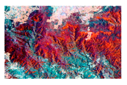 | ||
|---|---|---|---|
| (NIR/Red)-(SWIR1/NIR) | (SWIR1/Green)-(SWIR1/Red) | (Red/Blue)-(SWIR1/Green) | Examples |
| * | * | * |  |
| * | / | * |  |
| * | * | / |  |
| * | / | / |  |
| / | / | / |  |
| / | * | / |  |
| / | / | * |  |
| / | * | * |  |
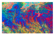
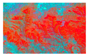
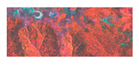
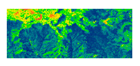
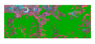
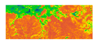
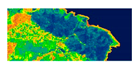
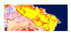
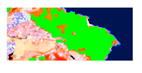
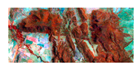
| Ontological Reference Image ‘Land/Water’ RGB | 15 m Aravena Rainforest Index in Pseudo Colour  | 15 m Aravena Rainforest Index Classification | 15 m Aravena Rainforest Band Ratio RGB Blend | 15 m Aravena Rainforest Band Ratio RGB Blend HSV Hue in Pseudo Colour  | 15 m Aravena Rainforest Band Ratio RGB Blend HSV Hue Classification | Existing 100 m Reference Classification on ‘Land/Water’ RGB |
|---|---|---|---|---|---|---|
| Example 1: Subtropical Rainforests; Location: 28.485 S, 152.716 E; Scale: 1:40,000. | ||||||
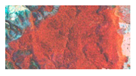 | 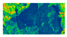 | 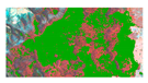 | 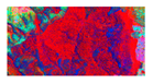 | 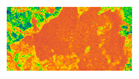 | 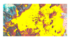 |  |
| Example 2: Northern Warm Temperate Rainforests; Location: 31.423 S, 152.134 E; Scale 1:60,000. | ||||||
 |  |  |  |  |  |  |
| Example 3: Southern Warm Temperate Rainforests; Location: 36.033 S, 149.880 E; Scale: 1:20,000. | ||||||
 |  |  |  |  |  |  |
| Example 4: Cool Temperate Rainforests; Location: 32.062 S, 151.481 E; Scale: 1:60,000. | ||||||
 |  |  |  |  |  |  |
| Example 5: Dry Rainforests; Location: 31.043 S, 152.214 E; Scale: 1:40,000. | ||||||
 |  |  |  |  |  |  |
| Example 6: Littoral (coastal) Rainforests; Location: 32.213 S, 152.553 E; Scale: 1:20,000. | ||||||
 |  |  |  |  |  |  |
| Example 7: Western Vine Thickets; Location: 29.661 S, 150.324 E; Scale: 1:30,000. | ||||||
 |  |  |  |  |  |  |
| Ecoregion | Indices (%) | Band Ratio RGB Hues (%) | |||||
|---|---|---|---|---|---|---|---|
| NDVI | EVI2 | NGRDI | Aravena Rainforest Index | SWIR1/Natural Colour Band Ratio RGB | SWIR1/Infrared Colour Band Ratio RGB | Aravena Rainforest Band Ratio RGB Blend | |
| North Coast | |||||||
| User Not Rainforest | 99.45 | 99.44 | 97.33 | 94.65 | 91.89 | 94.65 | 92.82 |
| User Rainforest | 13.17 | 14.97 | 40.72 | 55.09 | 59.88 | 48.50 | 62.87 |
| Producer Not Rainforest | 55.69 | 56.04 | 64.26 | 69.76 | 71.37 | 66.67 | 73.18 |
| Producer Rainforest | 95.65 | 95.65 | 93.51 | 90.52 | 87.08 | 89.20 | 88.89 |
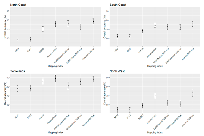
| Overall accuracy | 58.33 | 58.91 | 70.34 | 75.84 | 76.55 | 72.46 | 78.49 |
| South Coast | |||||||
| User Not Rainforest | 100 | 100 | 99.47 | 98.40 | 94.88 | 97.25 | 97.38 |
| User Rainforest | 13.61 | 14.29 | 28.57 | 43.54 | 43.54 | 40.14 | 47.62 |
| Producer Not Rainforest | 59.87 | 59.94 | 64.07 | 69.11 | 68.54 | 67.66 | 70.66 |
| Producer Rainforest | 100 | 100 | 97.62 | 95.45 | 87.14 | 91.53 | 93.59 |
| Overall accuracy | 62.21 | 62.28 | 68.26 | 74.34 | 72.62 | 72.24 | 75.80 |
| Tablelands and Rangelands | |||||||
| User Not Rainforest | 99.05 | 99.04 | 95.92 | 95.45 | 95.19 | 96.00 | 95.15 |
| User Rainforest | 38.18 | 38.18 | 67.27 | 76.36 | 54.55 | 65.45 | 74.55 |
| Producer Not Rainforest | 75.36 | 75.37 | 84.92 | 88.18 | 80.15 | 84.21 | 87.80 |
| Producer Rainforest | 95.45 | 95.45 | 89.47 | 89.80 | 85.71 | 89.47 | 89.13 |
| Overall accuracy | 77.99 | 78.05 | 86.03 | 88.69 | 81.33 | 85.35 | 88.13 |
| Northwest Slopes | |||||||
| User Not Rainforest | 100 | 100 | 100 | 98.36 | 100 | 98.46 | 96.72 |
| User Rainforest | 0 | 0 | 10.71 | 35.71 | 17.86 | 16.07 | 44.64 |
| Producer Not Rainforest | 54.47 | 54.47 | 57.26 | 64.71 | 58.93 | 58.41 | 67.71 |
| Producer Rainforest | 0 | 0 | 100 | 94.74 | 100 | 88.89 | 91.83 |
| Overall accuracy | 54.47 | 54.47 | 59.17 | 69.67 | 61.90 | 60.80 | 72.95 |
References
- Ali, I.; Greifeneder, F.; Stamenkovic, J.; Neumann, M.; Notarnicola, C. Review of Machine Learning Approaches for Biomass and Soil Moisture Retrievals from Remote Sensing Data. Remote Sens. 2015, 7, 16398–16421. [Google Scholar] [CrossRef] [Green Version]
- Fassnacht, F.; Latifi, H.; Stereńczak, K.; Modzelewska, A.; Lefsky, M.; Waser, L.; Straub, C.; Ghosh, A. Review of studies on tree species classification from remotely sensed data. Remote Sens. Environ. 2016, 186, 64–87. [Google Scholar] [CrossRef]
- Ball, J.E.; Anderson, D.T.; Chan, C.S. Comprehensive survey of deep learning in remote sensing: Theories, tools, and challenges for the community. J. Appl. Remote Sens. 2017, 11, 042609. [Google Scholar] [CrossRef] [Green Version]
- Janik, A.; Sankaran, K.; Ortiz, A. Interpreting Black-Box Semantic Segmentation Models in Remote Sensing Applications; Archambault, D., Nabney, I., Peltonen, J., Eds.; Machine Learning Methods in Visualisation for Big Data: Porto, Portugal, 2019. [Google Scholar]
- Roscher, R.; Bohn, B.; Duarte, M.F.; Garcke, J. Explain it to me—Facing remote sensing challenges in the bio- and geosciences with explainable machine learning. ISPRS Ann. Photogramm. Remote Sens. Spat. Inf. Sci. 2020, 3, 817–824. [Google Scholar] [CrossRef]
- Carvalho, D.V.; Pereira, E.M.; Cardoso, J.S. Machine Learning Interpretability: A Survey on Methods and Metrics. Electronics 2019, 8, 832. [Google Scholar] [CrossRef] [Green Version]
- Kovalerchuk, B.; Ahmad, M.A.; Teredesai, A. Survey of Explainable Machine Learning with Visual and Granular Methods Beyond Quasi-Explanations. Econom. Financ. Appl. 2021. [Google Scholar] [CrossRef]
- Campos-Taberner, M.; García-Haro, F.J.; Martínez, B.; Izquierdo-Verdiguier, E.; Atzberger, C.; Camps-Valls, G.; Gilabert, M.A. Understanding deep learning in land use classification based on Sentinel-2 time series. Sci. Rep. 2020, 10, 1–12. [Google Scholar] [CrossRef] [PubMed]
- Chatzimparmpas, A.; Martins, R.M.; Jusufi, I.; Kerren, A. A survey of surveys on the use of visualization for interpreting machine learning models. Inf. Vis. 2020, 19, 207–233. [Google Scholar] [CrossRef] [Green Version]
- Wester, K.; Lundén, B.; Bax, G. Analytically processed Landsat TM images for visual geological interpretation in the northern Scandinavian Caledonides. ISPRS J. Photogramm. Remote Sens. 1990, 45, 442–460. [Google Scholar] [CrossRef]
- Pekel, J.-F.; Cottam, A.; Gorelick, N.; Belward, A.S. High-resolution mapping of global surface water and its long-term changes. Nature 2016, 540, 418–422. [Google Scholar] [CrossRef]
- Keim, D.; Andrienko, G.; Fekete, J.D.; Görg, C.; Kohlhammer, J.; Melançon, G. Visual Analytics: Definition, Process, and Challenges. In Information Visualization; Springer: Berlin/Heidelberg, Germany, 2008. [Google Scholar]
- Ray, R.G. Aerial Photographs in Geologic Interpretation and Mapping, Geological Survey Professional Paper 373; United States Government Printing Office: Washington, DC, USA, 1960. [Google Scholar]
- Fensham, R.; Fairfax, R. Aerial photography for assessing vegetation change: A review of applications and the relevance of findings for Australian vegetation history. Aust. J. Bot. 2002, 50, 415–429. [Google Scholar] [CrossRef]
- Horning, N. Justification for Using Photo Interpretation Methods to Interpret Satellite Imagery Version 1.0; American Museum of Natural History, Center for Biodiversity and Conservation: New York, NY, USA, 2004. [Google Scholar]
- Morgan, J.L.; Gergel, S.E.; Coops, N. Aerial Photography: A Rapidly Evolving Tool for Ecological Management. Bioscience 2010, 60, 47–59. [Google Scholar] [CrossRef]
- White, R. Human expertise in the interpretation of remote sensing data: A cognitive task analysis of forest disturbance attribution. Int. J. Appl. Earth Obs. Geoinf. 2019, 74, 37–44. [Google Scholar] [CrossRef]
- Bey, A.; Díaz, A.S.-P.; Maniatis, D.; Marchi, G.; Mollicone, D.; Ricci, S.; Bastin, J.-F.; Moore, R.; Federici, S.; Rezende, M.; et al. Collect Earth: Land Use and Land Cover Assessment through Augmented Visual Interpretation. Remote Sens. 2016, 8, 807. [Google Scholar] [CrossRef] [Green Version]
- Smuts, J.C. Holism and Evolution; Macmillan: New York, NY, USA, 1926. [Google Scholar]
- Zonneveld, I.S. The land unit – A fundamental concept in landscape ecology, and its applications. Landsc. Ecol. 1989, 3, 67–86. [Google Scholar] [CrossRef]
- Avery, E.T.; Berlin, G.L. Fundamentals of Remote Sensing and Airphoto Interpretation; Macmillan: Stuttgart, Germany, 2003. [Google Scholar]
- White, R.A.; Çöltekin, A.; Hoffman, R.R. Remote Sensing and Cognition: Human Factors in Image Interpretation, 1st ed.; CRC Press: Boca Raton, FL, USA, 2018. [Google Scholar]
- Glenn, E.P.; Huete, A.R.; Nagler, P.L.; Nelson, S.G. Relationship Between Remotely-sensed Vegetation Indices, Canopy Attributes and Plant Physiological Processes: What Vegetation Indices Can and Cannot Tell Us About the Landscape. Sensors 2008, 8, 2136–2160. [Google Scholar] [CrossRef] [PubMed] [Green Version]
- Metcalfe, D.; Green, P. Chapter 15. Rainforests and Vine Thickets. In Australian Vegetation, 3rd ed.; Keith, D., Ed.; Wiley: Hoboken, NJ, USA, 2017; p. 766. [Google Scholar]
- Sultan, M.; Arvidson, R.E.; Sturchio, N.C.; Guinness, E.A. Lithologic mapping in arid regions with Landsat thematic mapper data: Meatiq dome, Egypt. Geol. Soc. Am. Bull. 1987, 99, 748–762. [Google Scholar] [CrossRef]
- Horning, N. Selecting the Appropriate Band Combination for an RGB Image Using Landsat Imagery Version 1.0; American Museum of Natural History, Center for Biodiversity and Conservation: New York, NY, USA, 2004. [Google Scholar]
- Van der Meer, F.D.; Van der Werff, H.M.; Van Ruitenbeek, F.J.; Hecker, C.A.; Bakker, W.H.; Noomen, M.F.; van der Meijde, M.; Carranza, E.J.M.; de Smeth, J.B.; Woldai, T. Multi-and Hyperspectral geologic remote sensing: A review. Int. J. Appl. Earth Obs. Geoinf. 2012, 14, 112–128. [Google Scholar] [CrossRef]
- Jensen, J.R. Biophysical Remote Sensing. Ann. Assoc. Am. Geogr. 1983, 73, 111–132. [Google Scholar] [CrossRef]
- Estes, J.E.; Hajic, E.J.; Tinney, L.R. Fundamentals of image analysis: Analysis of visible and thermal infrared data. In Manual of Remote Sensing; Colwell, R.N., Ed.; American Society of Photogrammetry: Falls Church, VI, USA, 1983. [Google Scholar]
- Campbell, J.B. Introduction to Remote Sensing; Guiliford Press: New York, NY, USA, 2002. [Google Scholar]
- Bianchetti, R.A.; MacEachren, A.M. Cognitive Themes Emerging from Air Photo Interpretation Texts Published to 1960. ISPRS Int. J. Geoinf. 2015, 4, 551–571. [Google Scholar] [CrossRef] [Green Version]
- Joblove, G.H.; Greenberg, D. Color spaces for computer graphics. ACM SIGGRAPH Comput. Graph. 1978, 12, 20–25. [Google Scholar] [CrossRef]
- Movia, A.; Beinat, A.; Sandri, T. Land use classification from VHR aerial images using invariant colour components and texture. ISPRS Int. Arch. Photogramm. Remote Sens. Spat. Inf. Sci. 2016, 41, 311–317. [Google Scholar] [CrossRef] [Green Version]
- Pekel, J.-F.; Ceccato, P.; Vancutsem, C.; Cressman, K.; Vanbogaert, E.; Defourny, P. Development and Application of Multi-Temporal Colorimetric Transformation to Monitor Vegetation in the Desert Locust Habitat. IEEE J. Sel. Top. Appl. Earth Obs. Remote Sens. 2011, 4, 318–326. [Google Scholar] [CrossRef]
- Wu, S.; Chen, H.; Zhao, Z.; Long, H.; Song, C. An Improved Remote Sensing Image Classification Based on K-Means Using HSV Color Feature. In Proceedings of the 10th International Conference on Computational Intelligence and Security, CIS 2014, Kunming, China, 15–16 November 2014; pp. 201–204. [Google Scholar]
- Lessel, J.; Ceccato, P. Creating a basic customizable framework for crop detection using Landsat imagery. Int. J. Remote Sens. 2016, 37, 6097–6107. [Google Scholar] [CrossRef]
- Pekel, J.-F.; Vancutsem, C.; Bastin, L.; Clerici, M.; Vanbogaert, E.; Bartholomé, E.; Defourny, P. A near real-time water surface detection method based on HSV transformation of MODIS multi-spectral time series data. Remote Sens. Environ. 2014, 140, 704–716. [Google Scholar] [CrossRef] [Green Version]
- Bertels, L.; Smets, B.; Wolfs, D. Dynamic Water Surface Detection Algorithm Applied on PROBA-V Multispectral Data. Remote Sens. 2016, 8, 1010. [Google Scholar] [CrossRef] [Green Version]
- Namikawa, L.; Körting, T.; Castejon, E. Water body extraction from RapidEye images: An automated methodology based on Hue component of color transformation from RGB to HSV model. Braz. J. Cartogr. 2016, 68, 1097–1111. [Google Scholar]
- Woerd, H.; Wernand, M. Hue-Angle Product for Low to Medium Spatial Resolution Optical Satellite Sensors. Remote Sens. 2018, 10, 180. [Google Scholar] [CrossRef] [Green Version]
- Lehmann, M.K.; Nguyen, U.; Allan, M.; Van Der Woerd, H.J. Colour Classification of 1486 Lakes across a Wide Range of Optical Water Types. Remote Sens. 2018, 10, 1273. [Google Scholar] [CrossRef] [Green Version]
- Zhao, Y.; Shen, Q.; Wang, Q.; Yang, F.; Wang, S.; Li, J.; Zhang, F.; Yao, Y. Recognition of Water Colour Anomaly by Using Hue Angle and Sentinel 2 Image. Remote Sens. 2020, 12, 716. [Google Scholar] [CrossRef] [Green Version]
- Cushman, S.A.; Littell, J.; McGarigal, K. The Problem of Ecological Scaling in Spatially Complex, Nonequilibrium Ecological Systems. In Spatial Complexity, Informatics, and Wildlife Conservation; Springer: Tokyo, Japan, 2010. [Google Scholar]
- Tran, B.N.; Tanase, M.A.; Bennett, L.T.; Aponte, C. Evaluation of Spectral Indices for Assessing Fire Severity in Australian Temperate Forests. Remote Sens. 2018, 10, 1680. [Google Scholar] [CrossRef] [Green Version]
- Stoian, A.; Poulain, V.; Inglada, J.; Poughon, V.; Derksen, D. Land Cover Maps Production with High Resolution Satellite Image Time Series and Convolutional Neural Networks: Adaptations and Limits for Operational Systems. Remote Sens. 2019, 11, 1986. [Google Scholar] [CrossRef] [Green Version]
- Wedding, L.M.; Lepczyk, C.A.; Pittman, S.J.; Friedlander, A.M.; Jorgensen, S. Quantifying seascape structure: Extending terrestrial spatial pattern metrics to the marine realm. Mar. Ecol. Prog. Ser. 2011, 427, 219–232. [Google Scholar] [CrossRef] [Green Version]
- Lewis, D.; Phinn, S. Accuracy assessment of vegetation community maps generated by aerial photography interpretation: Perspective from the tropical savanna, Australia. J. Appl. Remote Sens. 2011, 5, 053565. [Google Scholar] [CrossRef] [Green Version]
- Helmer, E.H.; Nicholas, R.; Goodwin, V.G.; Carlos, M.S., Jr.; Gregory, P.A. Characterizing tropical forests with multispectral imagery. In Land Resources: Monitoring, Modeling and Mapping; Thenkabail, P.S., Ed.; Taylor & Francis Group: Boca Raton, FL, USA, 2015; p. 849. [Google Scholar]
- Gorelick, N.; Hancher, M.; Dixon, M.; Ilyushchenko, S.; Thau, D.; Moore, R. Google Earth Engine: Planetary-scale geospatial analysis for everyone. Remote Sens. Environ. 2017, 202, 18–27. [Google Scholar] [CrossRef]
- Jelinski, D.; Wu, J. The Modifiable Areal Unit Problem and Implications for Landscape Ecology. Landsc. Ecol. 1996, 11, 129–140. [Google Scholar] [CrossRef]
- Roleček, J.; Chytrý, M.; Hájek, M.; Lvončík, S.; Tichý, L. Sampling design in large-scale vegetation studies: Do not sacrifice ecological thinking to statistical purism! Folia Geobot. Phytotaxon. 2007, 42, 199–208. [Google Scholar] [CrossRef] [Green Version]
- Guberman, S.; Maximov, V.; Pashintsev, A. Gestalt and Image Understanding. Gestalt Theory 2012, 34, 143. [Google Scholar]
- Deng, X.; Li, W.; Liu, X.; Guo, Q.; Newsam, S. One-class remote sensing classification: One-class vs. binary classifiers. Int. J. Remote Sens. 2018, 39, 1890–1910. [Google Scholar] [CrossRef]
- Rajbhandari, S.; Aryal, J.; Osborn, J.; Lucieer, A.; Musk, R. Leveraging Machine Learning to Extend Ontology-Driven Geographic Object-Based Image Analysis (O-GEOBIA): A Case Study in Forest-Type Mapping. Remote Sens. 2019, 11, 503. [Google Scholar] [CrossRef] [Green Version]
- Kumar, L.; Schmidt, K.S.; Dury, S.; Skidmore, A.K. Review of hyperspectral remote sensing and vegetation Science. In Imaging Spectrometry: Basic Principles and Prospective Applications; Van Der Meer, F.D., De Jong, S.M., Eds.; Kluwer: Dordrecht, The Netherlands, 2001. [Google Scholar]
- Thenkabail, P.S.; Hall, J.; Lin, T.; Ashton, M.S.; Harris, D.; Enclona, E.A. Detecting floristic structure and pattern across topographic and moisture gradients in a mixed species Central African forest using IKONOS and Landsat-7 ETM+ images. Int. J. Appl. Earth Obs. Geoinf. 2003, 4, 255–270. [Google Scholar] [CrossRef]
- Pasquarella, V.; Holden, C.E.; Kaufman, L.; Woodcock, C.E. From imagery to ecology: Leveraging time series of all available Landsat observations to map and monitor ecosystem state and dynamics. Remote Sens. Ecol. Conserv. 2016, 2, 152–170. [Google Scholar] [CrossRef]
- Chavez, P.S., Jr.; Berlin, G.L.; Sowers, L.B. Statistical method for selecting Landsat MSS ratios. J. Appl. Photogr. Eng. 1982, 8, 23–30. [Google Scholar]
- Sheffield, C. Selecting band combinations from multispectral data. Photogramm. Eng. Remote Sens. 1985, 51, 681–687. [Google Scholar]
- Saha, S.K.; Kudrat, M. Selection of spectral band combination for land cover/land use classification using a brightness value overlapping index (BVOI). J. Indian Soc. Remote Sens. 1991, 19, 141–147. [Google Scholar] [CrossRef]
- Beauchemin, M.; Fung, K.B. On statistical band selection for image visualization. Photogramm. Eng. Remote Sens. 2001, 67, 571–574. [Google Scholar]
- Ming, D.; Du, J.; Zhang, X.; Liu, T. Modified average local variance for pixel-level scale selection of multiband remote sensing images and its scale effect on image classification accuracy. J. Appl. Remote Sens. 2013, 7, 073565. [Google Scholar] [CrossRef]
- Miller, S.D.; Lindsey, D.T.; Seaman, C.J.; Solbrig, J.E. GeoColor: A Blending Technique for Satellite Imagery. J. Atmos. Ocean. Technol. 2020, 37, 429–448. [Google Scholar] [CrossRef]
- Sanchez, H.C.; Boyd, D.; Foody, G. One-Class Classification for Mapping a Specific Land-Cover Class: SVDD Classification of Fenland. IEEE Trans. Geosci. Remote Sens. 2007, 45, 1061–1073. [Google Scholar] [CrossRef] [Green Version]
- Bennett, M.W.A. Rapid monitoring of wetland water status using density slicing. In Proceedings of the 4th Australasian Remote Sensing Conference, Adelaide, Australia, 14–18 September 1987; pp. 682–691. [Google Scholar]
- Frazier, P.S.; Page, K.J. Water Body Detection and Delineation with Landsat TM Data. Photogramm. Eng. Remote Sens. 2000, 66, 1461–1467. [Google Scholar]
- Hamandawana, H.; Eckardt, F.; Ringrose, S. The use of step-wise density slicing in classifying high-resolution panchromatic photographs. Int. J. Remote Sens. 2006, 27, 4923–4942. [Google Scholar] [CrossRef]
- Yang, X.; Tien, D. An automated image analysis approach for classification and mapping of woody vegetation from digital aerial photograph. World Rev. Sci. Technol. Sustain. Dev. 2010, 7, 13–23. [Google Scholar] [CrossRef] [Green Version]
- Brewer, C.K.; Winne, J.C.; Redmond, R.L.; Opitz, D.W.; Mangrich, M.V. Classifying and Mapping Wildfire Severity. Photogramm. Eng. Remote Sens. 2005, 71, 1311–1320. [Google Scholar] [CrossRef] [Green Version]
- Laurance, W.F. Emerging Threats to Tropical Forests. Ann. Mo. Bot. Gard. 2015, 100, 159–169. [Google Scholar] [CrossRef]
- Laurance, S. An Amazonian rainforest and its fragments as a laboratory of global change. Biol. Rev. 2017, 93, 223–247. [Google Scholar] [CrossRef]
- Mayaux, P.; Pekel, J.-F.; Desclée, B.; Donnay, F.; Lupi, A.; Frédéric, A.; Clerici, M.; Bodart, C.; Brink, A.; Nasi, R.; et al. State and evolution of the African rainforests between 1990 and 2010. Philos. Trans. R. Soc. Lond. Ser. B Biol. Sci. 2013, 368, 20120300. [Google Scholar] [CrossRef] [Green Version]
- Australian Government Department of Agriculture, Water and the Environment. NVIS (National Vegetation Information System) V5.1 ©; Australian Government Department of Agriculture, Water and the Environment: Canberra, Australia, 2018. [Google Scholar]
- Montreal Process Implementation Group for Australia and National Forest Inventory Steering Committee. Australia’s State of the Forests Report 2018; ABARES: Canberra, Australia, 2018. [Google Scholar]
- Keith, D. Ocean Shores to Desert Dunes: The Native Vegetation of New South Wales and the ACT. TAXON 2005, 54, 1120. [Google Scholar]
- Keith, D.; Simpson, C. Vegetation Formations and Classes of NSW (Version 3.03), VIS_ID 3848; Department of Planning, Industry and Environment: Canberra, Australia, 2018. [Google Scholar]
- Webb, L.J. A Physiognomic Classification of Australian Rain Forests. J. Ecol. 1959, 47, 551–570. [Google Scholar] [CrossRef] [Green Version]
- Bowman, D.M.J.S. Australian Rainforest: Island of Green in a Land of Fire; Cambridge University Press: Cambridge, UK, 2000. [Google Scholar]
- Australian Government, Department of Environment and Energy. 2017: NVIS Fact Sheet MVG 1—Rainforests and Vine Thickets; Australian Government, Department of Environment and Energy: Canberra, Australia, 2017. [Google Scholar]
- Department of Agriculture, Water and the Environment. Interim Biogeographic Regionalisation for Australia (IBRA v7) Subregions—States and Territories; Department of Agriculture, Water and the Environment: Canberra, Australia, 2012. [Google Scholar]
- Sinha, P.; Kumar, L.; Reid, N. Seasonal Variation in Land-Cover Classification Accuracy in a Diverse Region. Photogramm. Eng. Remote Sens. 2012, 78, 271–280. [Google Scholar] [CrossRef]
- Huete, A.R.; Didan, K.; Shimabukuro, Y.E.; Ratana, P.; Saleska, S.R.; Hutyra, L.R.; Yang, W.; Nemani, R.R.; Myneni, R. Amazon rainforests green-up with sunlight in dry season. Geophys. Res. Lett. 2006, 33. [Google Scholar] [CrossRef] [Green Version]
- Ruefenacht, B. Comparison of Three Landsat TM Compositing Methods: A Case Study Using Modeled Tree Canopy Cover. Photogramm. Eng. Remote Sens. 2016, 82, 199–211. [Google Scholar] [CrossRef]
- Phan, T.N.; Kuch, V.; Lehnert, L. Land Cover Classification using Google Earth Engine and Random Forest Classifier—The Role of Image Composition. Remote Sens. 2020, 12, 2411. [Google Scholar] [CrossRef]
- Fisher, A.; Day, M.; Gill, T.; Roff, A.; Danaher, T.; Flood, N. Large-Area, High-Resolution Tree Cover Mapping with Multi-Temporal SPOT5 Imagery, New South Wales, Australia. Remote Sens. 2016, 8, 515. [Google Scholar] [CrossRef] [Green Version]
- Gillieson, D.; Lawson, T.J.; Searle, L. Applications of High Resolution Remote Sensing in Rainforest Ecology and Management. Living A Dyn. Trop. For. Landsc. 2009, 334–348. [Google Scholar] [CrossRef]
- Sesnie, S.E.; Finegan, B.; Gessler, P.E.; Thessler, S.; Bendana, Z.R.; Smith, A.M.S. The multispectral separability of Costa Rican rainforest types with support vector machines and Random Forest decision trees. Int. J. Remote Sens. 2010, 31, 2885–2909. [Google Scholar] [CrossRef]
- Silva, F.B.; Shimabukuro, Y.E.; Aragao, L.E.; Anderson, L.O.; Pereira, G.; Cardozo, F.; Arai, E. Large-scale heterogeneity of Amazonian phenology revealed from 26-year long AVHRR/NDVI time-series. Environ. Res. Lett. 2013, 8, 024011. [Google Scholar] [CrossRef] [Green Version]
- Verheggen, A.; Mayaux, P.; de Wasseige, C.; Defourny, P. Mapping Congo Basin vegetation types from 300m and 1km multi-sensor time series for carbon stocks and forest areas estimation. Biogeosciences 2012, 9, 5061–5079. [Google Scholar] [CrossRef] [Green Version]
- Rocha, A.V.; Shaver, G.R. Advantages of a two band EVI calculated from solar and photosynthetically active radiation fluxes. Agric. For. Meteorol. 2009, 149, 1560–1563. [Google Scholar] [CrossRef]
- Zhang, X.; Friedl, M.; Tan, B.; Goldberg, M.; Yu, Y. Long-Term Detection of Global Vegetation Phenology from Satellite Instruments. Phenol. Clim. Chang. 2012. [Google Scholar] [CrossRef] [Green Version]
- Washington-Allen, R.; West, N.; Ramsey, R.; Efroymson, R. A Protocol for Retrospective Remote Sensing: Based Ecological Monitoring of Rangelands. Rangelands 2006, 59, 19–29. [Google Scholar] [CrossRef]
- NSW Government (2019) NSW BioNet. Office of Environment and Heritage. 2020. Available online: http://www.bionet.nsw.gov.au/ (accessed on 15 March 2021).
- Lyons, M.B.; Keith, D.A.; Phinn, S.R.; Mason, T.J.; Elith, J. A comparison of resampling methods for remote sensing classification and accuracy assessment. Remote Sens. Environ. 2018, 208, 145–153. [Google Scholar] [CrossRef]
- Department of Environment and Conservation. Natural Resource Management Field Assessment Guidelines—Rainforest Identification Field Guide; NSW: Canberra, Australia, 2004. [Google Scholar]
- Ustin, S.L.; Gamon, J.A. Remote sensing of plant functional types. New Phytol. 2010, 186, 795–816. [Google Scholar] [CrossRef]
- Brown, M.I.; Pearce, T.; Leon, J.; Sidle, R.; Wilson, R. Using remote sensing and traditional ecological knowledge (TEK) to understand mangrove change on the Maroochy River, Queensland, Australia. Appl. Geogr. 2018, 94, 71–83. [Google Scholar] [CrossRef]
- Eddy, I.M.; Gergel, S.E.; Coops, N.C.; Henebry, G.M.; Levine, J.; Zerriffi, H.; Shibkov, E. Integrating remote sensing and local ecological knowledge to monitor rangeland dynamics. Ecol. Indic. 2017, 82, 106–116. [Google Scholar] [CrossRef]
- Koskinen, J.; Leinonen, U.; Vollrath, A.; Ortmann, A.; Lindquist, E.; D’Annunzio, R.; Pekkarinen, A.; Käyhkö, N. Participatory mapping of forest plantations with Open Foris and Google Earth Engine. ISPRS J. Photogramm. Remote Sens. 2019, 148, 63–74. [Google Scholar] [CrossRef]
- Chavolla, E.; Zaldivar, D.; Cuevas, E.; Perez-Cisneros, M.A. Color Spaces Advantages and Disadvantages in Image Color Clustering Segmentation. Econom. Financ. Appl. 2017. [Google Scholar] [CrossRef]
- Fisher, N. Statistical Analysis of Circular Data; Cambridge University Press: Cambridge, UK, 1996. [Google Scholar]


| SII Visual Interpretation Key | |||||
|---|---|---|---|---|---|
| Example of Rainforest Type and Location | VHR GEE Imagery in ‘Natural Colour’ RGB | Sentinel 2 Image in ‘Land/Water’ RGB with the Same Linear stretch in GEE | Interpretation Ontology of General Appearance Consistent to the Same Image Stretch | Existing 100 m Resolution Classification Reference for Rainforests in Green | Sentinel 2 Image in ‘Land/Water’ RGB Enhanced with a Histogram Equalisation at the Current Extent in a GIS |
| Subtropical Rainforests Location: 28.673 S, 152.476 E Scale: 1:100,000 |  | 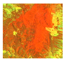 | Hue: Orange. Brightness: Average. Texture: Rough. Shape/size: Large. Association: Scattered along coastal lowlands & escarpment foothills, & may extend up escarpment gullies to altitudes of 900 m. |  | 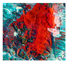 |
| Northern Warm Temperate Rainforests Location: 31.200 S, 152.386 E Scale: 1:100,000 | 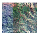 | 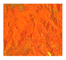 | Hue: Orange. Brightness: Average. Texture: Rough. Shape/size: Varying. Association: In hilly to steep terrain on coastal ranges & plateaux, & may extend above 1000 m. | 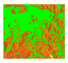 | 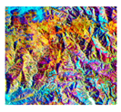 |
| Southern Warm Temperate Rainforests Location: 36.032 S, 149.897 E Scale: 1:80,000 |  | 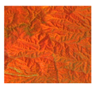 | Hue: Orange. Brightness: Bright. Texture: Smooth. Shape/size: Thin & tributary. Association: Typically in deep, moist, sheltered gullies among coastal ranges & foothills. |  | 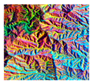 |
| Cool Temperate Rainforests Location: 32.067 S, 151.497 E Scale: 1:100,000 |  | 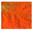 | Hue: Dark orange. Brightness: Duller. Texture: Rough. Shape/size: Varying. Association: High elevation above 900 m. | 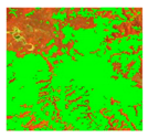 | 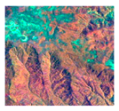 |
| Dry Rainforests Location: 31.054 S, 152.237 E Scale: 1:100,000 |  | 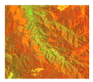 | Hue: Light orange. Brightness: Bright. Texture: Smooth. Shape/size: Patchy. Association: In rough terrain surrounded by Dry Sclerophylls. | 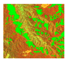 | 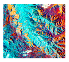 |
| Littoral (coastal) Rainforests Location: 32.431 S, 152.523 E Scale: 1:20,000 | 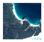 |  | Hue: Orange. Brightness: Bright. Texture: Smooth. Shape/size: Small, patchy or elongated. Association: Next to the ocean. | 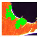 | 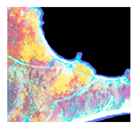 |
| Vine thickets in the Northwest Slopes Location: 29.696 S, 150.322 E Scale: 1:60,000 | 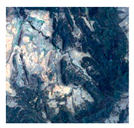 | 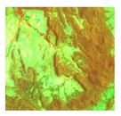 | Hue: Orange to brown. Brightness: Dull. Texture: Varying. Shape/size: Patchy of varying sizes & shape. Association: On flat to rolling terrain. | 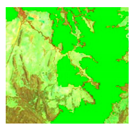 | 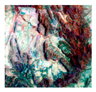 |
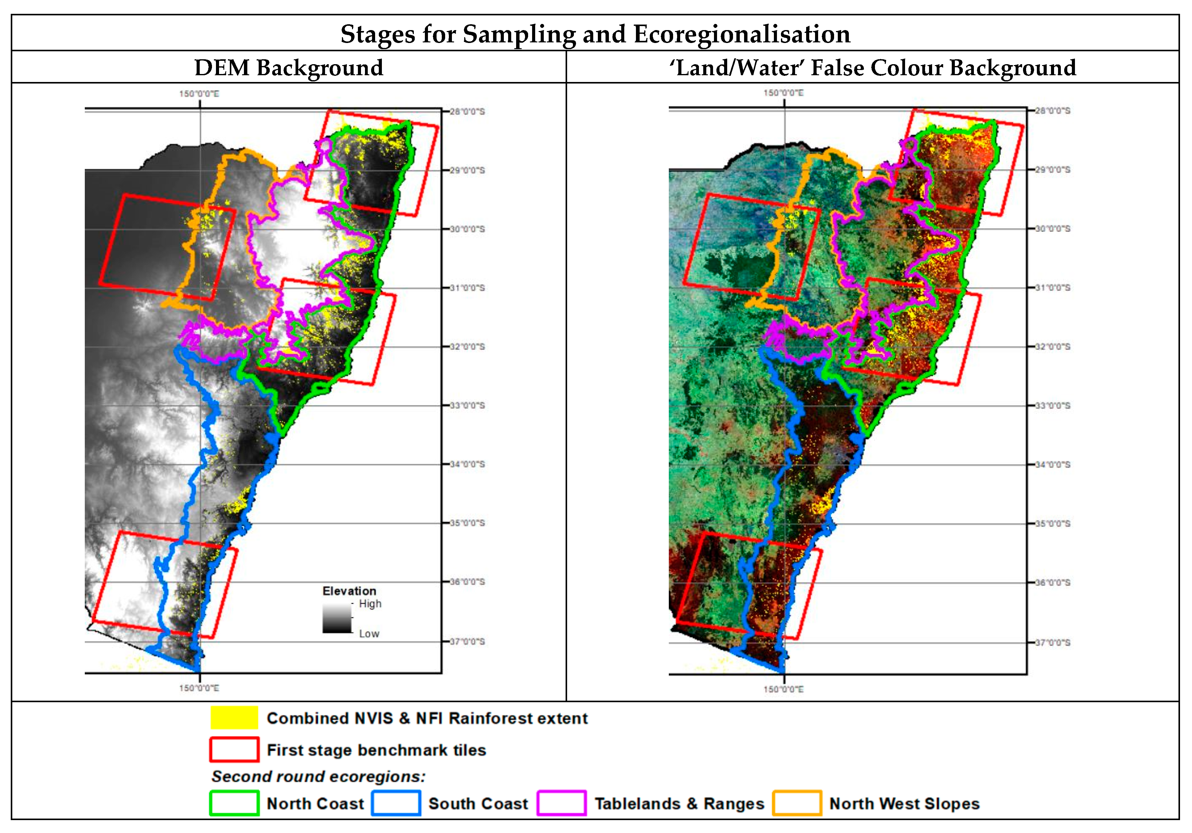
| Ecoregional Strata | Temporal Range for Interannual Composites |
|---|---|
| North Coast | November to December 2015–2018 |
| South Coast | December to January 2015–2018 |
| Tablelands and Ranges | November to January 2015–2018 |
| Northwest Slopes | January to February 2015–2018 |
| Candidate Indices Relative to Reference RGB | |||
|---|---|---|---|
| Reference RGB Visualisation (RGB: NIR, SWIR1, Red): Rainforest in Orange |  | ||
| Candidate Index | Equation or Hue Angle from an RGB Combination | Rationale for Testing | Examples (in Greyscale for Indices and as RGBs for False Colour Band Ratio Combinations) |
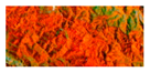
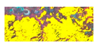
| NDVI | (NIR-Red)/(NIR+Red) | Commonly used vegetation index for maps with rainforests or closed tropical evergreen forests from the past [86,87,88]. |  Rainforest in white |
| EVI 2 | 2.4*(NIR-Red)/(NIR+Red+1) | Two band functional equivalent to the EVI, commonly used in tropical forest studies [89]. EVI 2 has been shown to be less sensitive to background reflectance, including bright soils and non-photosynthetically active vegetation [90,91]. | 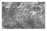 Rainforest in white |
| NGRDI | (Green-Red)/(Green+Red) | Replacing the NIR band (in NDVI) with the Green band appears to reduce the high value saturation produced by NDVI. | 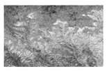 Rainforest in white |
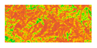
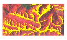
| # Aravena Rainforest Index | (SWIR1/Red)-(SWIR1/Green) | A compromise between the wider spectral range and the lower resolution of the SWIR1 band, subtracting feature related band ratios of SWIR1, where the Red and Green bands are derived from the NGRDI. |  Rainforest in white |
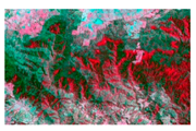
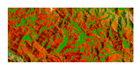
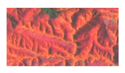
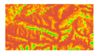
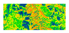
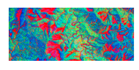
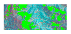
| # SWIR1/Natural Colour Band Ratio RGB hue | Hue angle from band ratio R,G,B: SWIR1/Red, SWIR1/Green, SWIR1/Blue | A distinct hue from a band ratio RGB combination, differentiating the SWIR1 band which displays the highest water absorption, with the bands from the ‘Natural Colour’ RGB combination to include structural and greenness data and narrow down and emphasise the moisture and brightness characteristic of rainforests compared to other forest types. | 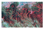 Rainforest in orange |
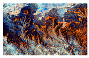
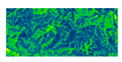
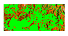
| # SWIR1/Infrared Colour Band Ratio RGB hue | Hue angle from band ratio R,G,B: SWIR1/NIR, SWIR1/Red, SWIR1/Green | A distinct hue from a band ratio RGB differentiating the SWIR1 band with the bands from the ‘Infrared Colour’ RGB combination to include structural, greenness and wetness data. |  Rainforest in green |
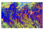
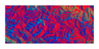
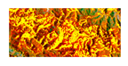
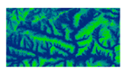
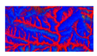
| # Aravena Rainforest Band Ratio RGB Blend hue | Hue angle from band ratio R,G,B: SWIR1/Red, Red/Green, (Red/Blue)/(SWIR1/Green) | A distinct hue from a band ratio RGB blend, selectively multiplying or dividing band ratios to produce the maximum spectral separability between rainforests and all other features in the landscape. |  Rainforest in red |
| Indices (%) | Band Ratio RGB Hues (%) | ||||||
|---|---|---|---|---|---|---|---|
| Ecoregions | NDVI | EVI2 | NGRDI | Aravena Rainforest Index | SWIR1/Natural Colour Band Ratio RGB | SWIR1/Infrared Colour Band Ratio RGB | Aravena Rainforest Band Ratio RGB Blend |
| North Coast | 58.27 | 58.91 | 70.25 | 75.78 | 76.60 | 72.47 | 78.51 |
| South Coast | 62.20 | 62.28 | 68.28 | 74.33 | 72.65 | 72.27 | 75.74 |
| Tablelands and Ranges | 77.91 | 77.98 | 85.98 | 88.54 | 81.37 | 85.35 | 88.02 |
| Northwest Slopes | 54.47 | 54.47 | 59.02 | 69.77 | 61.98 | 60.83 | 72.95 |
 | |||||||
| Ecoregions | Total Area From Existing 100 m Resolution Combined NVIS and NFI Classification (Ha) | Total from 15 m Resolution Classification from This Study (Ha) | Percentage Difference | Index Used |
|---|---|---|---|---|
| North Coast | 385,902 | 395,238 | 2.4% more | Aravena Rainforest Band Ratio RGB Blend |
| South Coast | 120,779 | 82,564 | 31.6% less | Aravena Rainforest Band Ratio RGB Blend |
| Tablelands and Ranges | 198,924 | 257,819 | 29.6% more | Aravena Rainforest Index |
| Northwest Slopes | 57,470 | 28,726 | 50% less | Aravena Rainforest Band Ratio RGB Blend |
| Index or Hue | Area and % of Agriculture Misclassified as Rainforest by Ecoregion | |||||||
|---|---|---|---|---|---|---|---|---|
| North Coast | South Coast | Tablelands and Ranges | Northwest Slopes | |||||
| Area (Ha) | % | Area (Ha) | % | Area (Ha) | % | Area (Ha) | % | |
| SWIR1/Natural Colour Band Ratio RGB Hue | 218,190 | 55.2 | 95,850 | 116.1 | 104,781 | 40.6 | 39,746 | 138.4 |
| Aravena Rainforest Band Ratio RGB Blend Hue | 31,478 | 8 | 24,101 | 29.2 | 68,030 | 26.4 | 25,163 | 87.6 |
| Aravena Rainforest Index | 17,386 | 4.4 | 15,168 | 18.4 | 53,163 | 20.6 | 20,895 | 72.7 |
| SWIR1/Infrared Colour Band Ratio RGB Hue | 7809 | 2 | 5735 | 6.9 | 7399 | 2.9 | 5654 | 19.7 |
| EVI 2 | 3231 | 0.8 | 739 | 0.9 | 3623 | 1.4 | 9495 | 33.1 |
| NDVI | 3046 | 0.8 | 686 | 0.8 | 3475 | 1.3 | 9208 | 32.1 |
| NGRDI | 2914 | 0.7 | 1071 | 1.3 | 7627 | 3 | 7863 | 27.4 |
Publisher’s Note: MDPI stays neutral with regard to jurisdictional claims in published maps and institutional affiliations. |
© 2021 by the authors. Licensee MDPI, Basel, Switzerland. This article is an open access article distributed under the terms and conditions of the Creative Commons Attribution (CC BY) license (https://creativecommons.org/licenses/by/4.0/).
Share and Cite
Aravena, R.A.; Lyons, M.B.; Roff, A.; Keith, D.A. A Colourimetric Approach to Ecological Remote Sensing: Case Study for the Rainforests of South-Eastern Australia. Remote Sens. 2021, 13, 2544. https://doi.org/10.3390/rs13132544
Aravena RA, Lyons MB, Roff A, Keith DA. A Colourimetric Approach to Ecological Remote Sensing: Case Study for the Rainforests of South-Eastern Australia. Remote Sensing. 2021; 13(13):2544. https://doi.org/10.3390/rs13132544
Chicago/Turabian StyleAravena, Ricardo A., Mitchell B. Lyons, Adam Roff, and David A. Keith. 2021. "A Colourimetric Approach to Ecological Remote Sensing: Case Study for the Rainforests of South-Eastern Australia" Remote Sensing 13, no. 13: 2544. https://doi.org/10.3390/rs13132544
APA StyleAravena, R. A., Lyons, M. B., Roff, A., & Keith, D. A. (2021). A Colourimetric Approach to Ecological Remote Sensing: Case Study for the Rainforests of South-Eastern Australia. Remote Sensing, 13(13), 2544. https://doi.org/10.3390/rs13132544