Remote Sensing-Based Statistical Approach for Defining Drained Lake Basins in a Continuous Permafrost Region, North Slope of Alaska

Abstract

Lake formation and drainage are pervasive phenomena in permafrost regions. Drained lake basins (DLBs) are often the most common landforms in lowland permafrost regions in the Arctic (50% to 75% of the landscape). However, detailed assessments of DLB distribution and abundance are limited. In this study, we present a novel and scalable remote sensing-based approach to identifying DLBs in lowland permafrost regions, using the North Slope of Alaska as a case study. We validated this first North Slope-wide DLB data product against several previously published sub-regional scale datasets and manually classified points. The study area covered >71,000 km², including a >39,000 km² area not previously covered in existing DLB datasets. Our approach used Landsat-8 multispectral imagery and ArcticDEM data to derive a pixel-by-pixel statistical assessment of likelihood of DLB occurrence in sub-regions with different permafrost and periglacial landscape conditions, as well as to quantify aerial coverage of DLBs on the North Slope of Alaska. The results were consistent with previously published regional DLB datasets (up to 87% agreement) and showed high agreement with manually classified random points (64.4–95.5% for DLB and 83.2–95.4% for non-DLB areas). Validation of the remote sensing-based statistical approach on the North Slope of Alaska indicated that it may be possible to extend this methodology to conduct a comprehensive assessment of DLBs in pan-Arctic lowland permafrost regions. Better resolution of the spatial distribution of DLBs in lowland permafrost regions is important for quantitative studies on landscape diversity, wildlife habitat, permafrost, hydrology, geotechnical conditions, and high-latitude carbon cycling.

1. Introduction

Permafrost-region lakes and drained lake basins (DLBs) are dominant landforms in Arctic lowland regions and play an important role in the geomorphological and ecological diversity of landscapes, as a wildlife habitat and for high-latitude carbon cycling [1,2,3,4,5]. Lakes and DLBs are prevalent landforms of the continuous permafrost zone in areas characterized by a high ground ice content (thermokarst lakes and drained thermokarst lake basins), as well as in areas with low to moderate ground ice content (mainly non-thermokarst lakes and drained lake basins) [6,7,8,9,10]. Local- to regional-scale studies in lowland ice-rich terrain have shown that the area of both lakes and DLBs can occupy 50% to 75% of the landscape [11], and that DLB coverage is typically two to three times higher than the areal coverage of extant lakes [12,13].

The presence of both lakes and DLBs and their relative distribution in the landscape have been the subject of numerous studies, which have also focused on their role in permafrost-region carbon cycling, habitat provision, and human land use practices. Thermokarst lakes are important landscape features due to their significant role in permafrost carbon mobilization [14,15,16], their role as freshwater sources that are critical for Arctic settlements and industry [17,18,19], and as an important habitat that supports resident and migratory wildlife [20,21].

Lake drainage and the formation of DLBs can be triggered through a wide range of mechanisms such as bank erosion of adjacent rivers, headward stream erosion, underground piping, bank overflow, or ice wedge degradation [22,23,24,25]. Drainage events are highly variable both spatially and temporally [26], though studies have shown a recent increase in the rate of lake drainage events in Arctic permafrost landscapes [27]. After lake drainage, DLBs become sites of plant colonization, peat accumulation, and permafrost aggradation and critical areas for carbon sequestration. Regionally, DLBs create a unique mosaic of tundra habitats characterized by various stages of post-drainage succession and diverse plant communities [2,22,28]. As such, accurately mapping both lakes and DLBs is critical for understanding how lowland permafrost regions in the Arctic may change in response to a warming climate [22].

Many studies have used remote sensing techniques to map permafrost-region lakes and DLBs [29,30,31]. Lakes and other surface water bodies can be mapped using multispectral and radar remote sensing technologies [26,32]. Remote sensing data have been used to study different characteristics of lakes such as morphometry (area, shape, orientation, length/width ratios) [7], ice coverage ratios, lake depth [33], lake ice formation, ice cover duration, methane ebullition, and ice regimes (floating ice, bedfast ice) [34,35,36,37,38,39,40]. Remote sensing can also be used to classify lake drainage mechanisms [27]. Through image time series analysis, abrupt decreases in surface water coverage can be interpreted, including lake initiation, growth, and shrinkage or drainage events [27,41]. Existing studies focusing on mapping DLBs are limited to local and regional scales [6,7,42]. Challenges in mapping DLBs arise from their spatial overlap with older generations of basins, a sometimes very shallow topography, and their spectral similarity to the surrounding tundra surfaces. Early studies using remote sensing data to map DLBs required significant manual interaction, such as digitizing basin perimeters by hand from satellite imagery [6,42]. Such approaches are not feasible for mapping DLBs over large areas or upscaling to the pan-Arctic. Automated and semi-automated approaches have been applied to selected areas in Alaska. Frohn et al. [6] classified DLBs on the western Arctic Coastal Plain of Alaska using image segmentation and Landsat-7 acquisitions from 2000–2002. Image segmentation proved to be a crucial part of their approach, as it considered the shapes of the image objects as opposed to relying solely on pixel-based approaches. Mapping of DLBs also relies on the successional patterns of vegetation, soils, and permafrost observed in basins after drainage, including barren ground in the first years, followed by wet fen development on lake sediments over the first decades, which is eventually succeeded by transitions to bogs and polygonal tundra vegetation over several centuries [7,10,43].

Expanding upon existing regional DLB datasets and working towards a pan-Arctic DLB dataset is a crucial step in furthering our understanding of Arctic landscapes on a circumpolar scale, as well as an important milestone for efforts seeking to upscale field measurements, such as carbon stocks and habitat change, and to better represent permafrost landscapes in Earth system models. To work towards pan-Arctic mapping of DLBs, a scalable mapping approach utilizing widely available data and accessible methodologies is necessary. In this study, we present a novel DLB mapping approach utilizing freely available data (Landsat imagery and the ArcticDEM), which can be readily transferred and scaled to other areas within the pan-Arctic permafrost region. This study provides the impetus and a framework for future large-scale mapping of DLB areas in lowland Arctic permafrost regions.

2. Materials and Methods

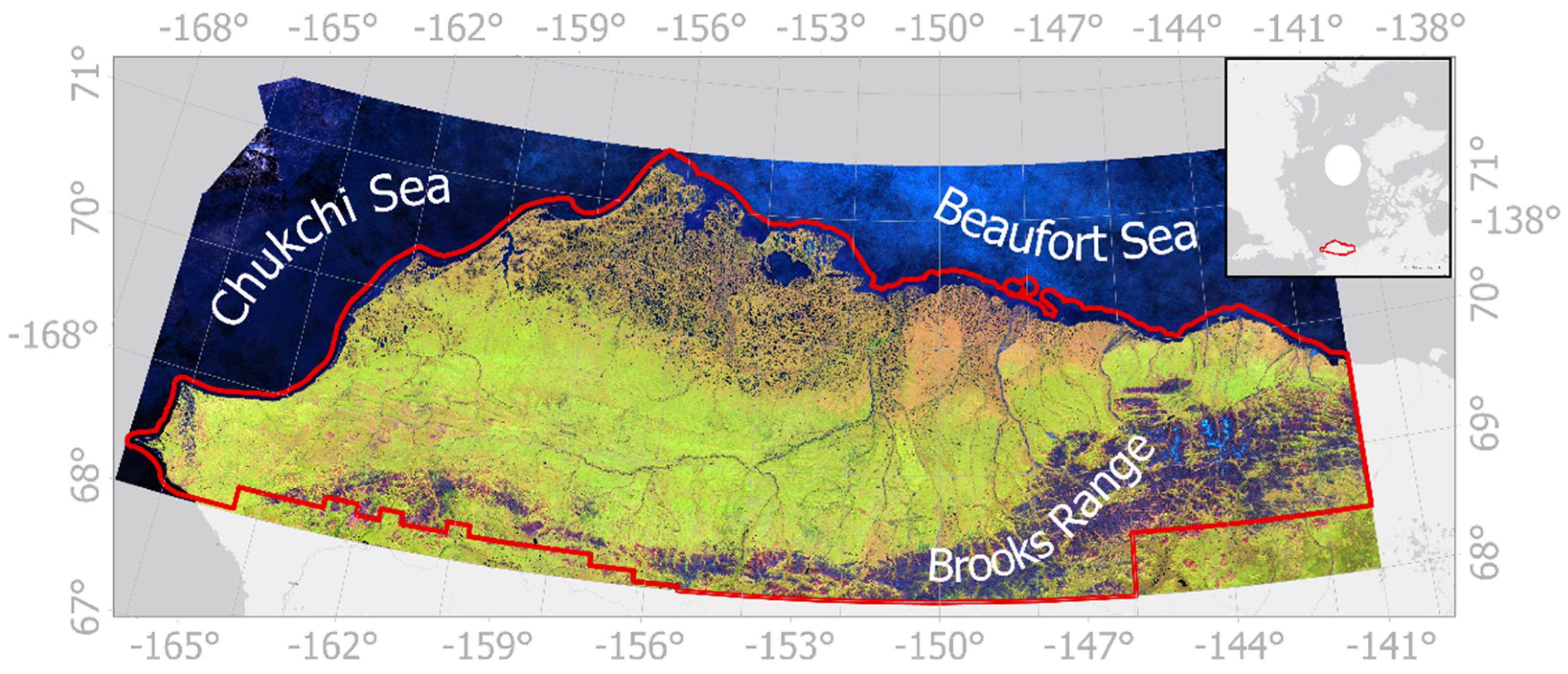
2.1. Study Area

In this study, we focus on the lake-rich region of the North Slope of Arctic Alaska, an area (>71,000 km²) that is delineated by the administrative borders of the North Slope Borough (see Figure 1) and the Canadian border, as well as natural borders such as the Brooks Range to the south and the Arctic Ocean (Beaufort and Chukchi sea) coastline to the north and west [44].

The North Slope region is underlaid by thick, continuous permafrost (200–600 m) [45]. The surficial geology (Figure 2) varies across the study region, with the most prevalent being aeolian silt, marine sand, and eolian sand [12]. High ground ice content occurs in regions underlaid by marine, fluvial, and eolian silt deposits with large ice wedges, ranging from 50 to 90% of the total volumetric ice content [9]. In these areas, development of thermokarst (surface subsidence caused by the melting of massive ground ice) is common [12,46]. In other areas with coarser sediment, such as sand and gravels, the permafrost tends to be less ice-rich, with less subsidence upon thawing. Lakes and DLBs in these regions are typically considered to be of non-thermokarst origin [9]. The active layer, being the ground surface layer that thaws during the summer and freezes during the winter, reaches from 20 cm to more than 100 cm thickness [45]. However, active layer thickness can vary greatly on a local level, being strongly influenced by local air and surface temperatures [47], the thermal conductivity of the soil, the thickness of the surficial organic mat, and snow thickness distribution. The North Slope region is characterized by numerous lakes, DLBs, and other thermokarst features [11]. Vegetation across the North Slope varies along a north to south gradient from the coast towards the Brooks Range [48]. Tundra vegetation is present across the region, with sedges, mosses and dwarf shrubs being dominant in lowland areas and tussock-forming sedges, dwarf shrubs, and mosses being dominant in uplands [48,49,50]. Vegetation varies between DLBs and the surrounding areas, as well as among DLBs of different drainage ages [42].

2.2. Data Selection and Pre-Processing

2.2.1. Landsat-8 Mosaic

In this study, we utilized Landsat-8 Tier-1 Top of Atmosphere (TOA) late summer imagery (August to mid-September) from 2014–2019 through Google Earth Engine (GEE) [51] to create a complete cloudless mosaic for the North Slope of Alaska. Landsat-8 provides multispectral data in multiple bands, including 3 bands in the visible spectrum, a near infrared band (NIR, 0.85–0.88 µm), and 2 short-wave infrared bands (SWIR, 1.57–1.65 µm; 2.11–2.29 µm) at a moderate spatial resolution (30 m). TOA imagery is necessary when working with Tassled Cap indices (as the coefficients are calibrated for TOA), which are described below. Mid- to late summer imagery was chosen to avoid early summer flooding caused by snow melt, which would lead to an overestimation of lake size and interfere with unambiguously defining DLBs. The Landsat-8 mosaic was filtered using a series of additional steps prior to analysis. First, to achieve the cloudless mosaic and to exclude pixels influenced by the presence of clouds, we took advantage of the Simple Cloud Score Algorithm, implemented in GEE. The algorithm computes a single cloud likelihood score (the likelihood of a pixel being cloud from 0 to 100), considering brightness, temperature, and the normalized difference snow index (NDSI) (https://developers.google.com/earth-engine/landsat; last accessed on 21 April 2021). The resulting cloud likelihood score is suitable for use as a simple cloud mask. Landsat-8 pixels with cloud likelihood scores below 20 were included in the mosaicking process. Other studies have limited their selection of pixels to those with cloud likelihood scores below 10 [52,53,54]; however, due to the scarcity of cloud-free Landsat acquisitions, we expanded the limit to include imagery with a cloud likelihood score of up to 20. Pixels fulfilling this criterion were used to create a median mosaic from all included imagery, taking the median value of each available pixel over the time series. Using the median value instead of the mean value served as a second step to exclude pixels that were outliers due to cloud influence or ephemeral flooding during a year with high precipitation. The resulting cloud-free Landsat-8 mosaic (Figure 1) was used for all further analyses in this study. To exclude water bodies, including lakes, rivers, and the ocean, we used the normalized difference water index (NDWI) with a threshold of 0.4 [55]. This threshold included both larger lakes as well as smaller surface water bodies, such as remnant lakes within partially drained basins. Finally, mountainous areas were masked from the Landsat-8 mosaic using a landform dataset presented in [56], which is further described in Section 2.2.3.

Figure 2. General geology of the study area based on [56], with gray areas representing areas outside of the study area.

Figure 2. General geology of the study area based on [56], with gray areas representing areas outside of the study area.

For the mapping of DLBs, the Tasseled Cap transformation (TCT) was derived from the cloud-free Landsat-8 mosaic. The TCT is a well-established multispectral transformation that provides information on the brightness, greenness, and wetness of a given pixel and has been successfully used to monitor Arctic landscapes [57,58], including the evolution of retrogressive thaw slumps [59], landcover changes [60], and lake drainage events [61]. We used the TCT coefficients published by Baig et al. [62] with the transformation coefficients as reported in

Table 1. Tasseled Cap transformation (TCT) coefficients for Landsat-8 for top-of-atmosphere reflectance values as published in [62].

Landsat-8 TCT	Blue Band 2	Green Band 3	Red 4 Band 4	NIR Band 5	SWIR1 Band 6	SWIR2 Band 7
Brightness	0.3029	0.2786	0.4733	0.5599	0.5080	0.1872
Greenness	−0.2941	−0.2430	−0.5424	0.7276	0.0713	−0.1608
Wetness	0.1511	0.1973	0.3283	0.3407	−0.7117	−0.4599
TCT4	−0.8239	0.0849	0.4396	−0.0580	0.2013	−0.2773
TCT5	−0.3294	0.0557	0.1056	0.1855	−0.4349	0.8085
TCT6	0.1079	−0.9023	0.4119	0.0575	−0.0259	0.0252

.

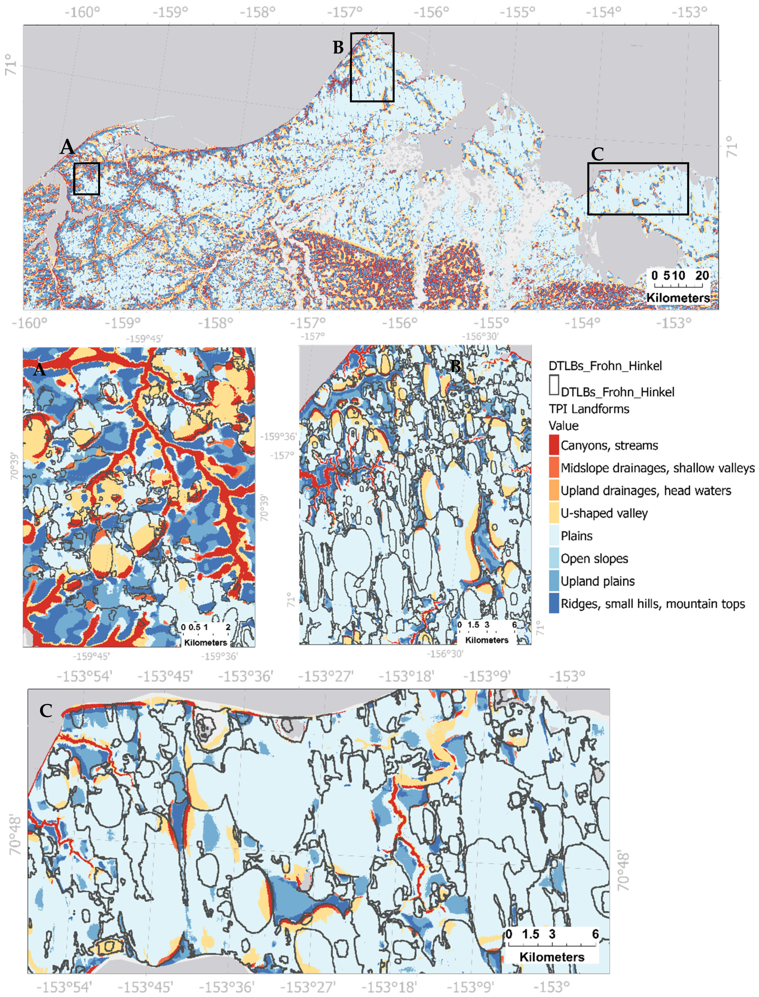
2.2.2. Landform Classification

To complement the spectral information from the Landsat-8 mosaic, we used the ArcticDEM [63] to develop a general landform classification. The ArcticDEM is a high-resolution circumpolar elevation dataset provided by the Polar Geospatial Center (PGC) [63]. ArcticDEM data were derived from high-resolution WorldView-1, WorldView-2, WorldView-3, and GeoEye-1 panchromatic stereo imagery. The ArcticDEM Mosaic product’s full resolution is 2 m, which we aggregated, using the median elevation value, to a 10 m digital elevation model (DEM) to minimize irregularities in the data, while still retaining a spatial resolution capable of resolving primary landform features. The ArcticDEM was also used because it covers the entire circumpolar region and allows for a future expansion of our workflow to other regions in the Arctic.

Based on an approach presented by Guisan et al. [64], Weiss [65] proposed a GIS-based landform classification approach based on the Topographic Position Index (TPI) or the difference from mean elevation (DIFF) as defined by Gallant and Wilson [66]. The TPI describes the relative topographic position of a point as the difference between its elevation and the mean elevation of a predetermined neighborhood with a set radius. The approach introduced by [65,66,67], and applied in a number of landscape-scale studies (e.g., [68,69,70,71]), allowed us to differentiate the study area into 10 distinct landform classes: (1) deeply incised streams, (2) mid-slope drainages and shallow valleys, (3) upland drainages and headwaters, (4) U-shaped valleys, (5) lowland plains, (6) open slopes, (7) upland plains, (8) local ridges/hills in valleys, (9) mid-slope ridges and small hills in plains, and (10) mountain tops and high ridges. In our study, we used this landform classification method through the ArcGIS extension published by [67] to create a TPI-based landform classification using the ArcticDEM for our study area (see

Table 2. The landform parameters (LPs) for the different landforms resulting from the Topographic Position Index (TPI), including the area (in %) which the different landforms occupy within and outside DLBs as classified by Frohn et al. [6].

Landforms	DLB Area Classified as Landform in %	Non-DLB Area Classified as Landform in %	Area % of Landform Classified as DLB	LP
Streams	10.5	13.7	22.9	0.7
Mid-slope drainages, shallow valleys	2.8	2.1	34.1	0.5
Upland drainages, head waters	0.3	0.6	16.3	0.4
U-shaped valleys	16.1	14.1	30.6	1
Plains	61.6	33.7	41.5	1
Open slopes	5.9	0.05	16.1	0.8
Upland plains	0.01	2.35	16.3	0.2
Local ridges, mid-slope ridges, small hills, mountain tops, high ridges	2.5	20.8	15.1	0

). The 10 landform classes resulting from this approach were adapted to better describe periglacial landforms, as this terminology differed from the terminology more commonly used in these settings. Landforms included in the analysis are shown in Figure 3.

2.2.3. Ancillary Geospatial Datasets

Maps detailing the surficial geology of the North Slope of Alaska published in Jorgenson et al. [56] were used to exclude mountainous areas, large rivers, and active floodplains from the data set prior to any statistical analysis. Previously published local and regional DLB datasets were used for comparison with our remote sensing-based statistical approach. These include data published in Frohn et al. [6] based on Landsat ETM+ data for the western Arctic Coastal Plain of Alaska, in Jones and Arp [11] for an area north of Teshekpuk Lake based on Landsat ETM+ data and an IfSAR digital surface model, and in Jones et al. [72] for an area within the Anaktuvuk River fire [73] area based on TPI analysis of down-sampled LiDAR data.

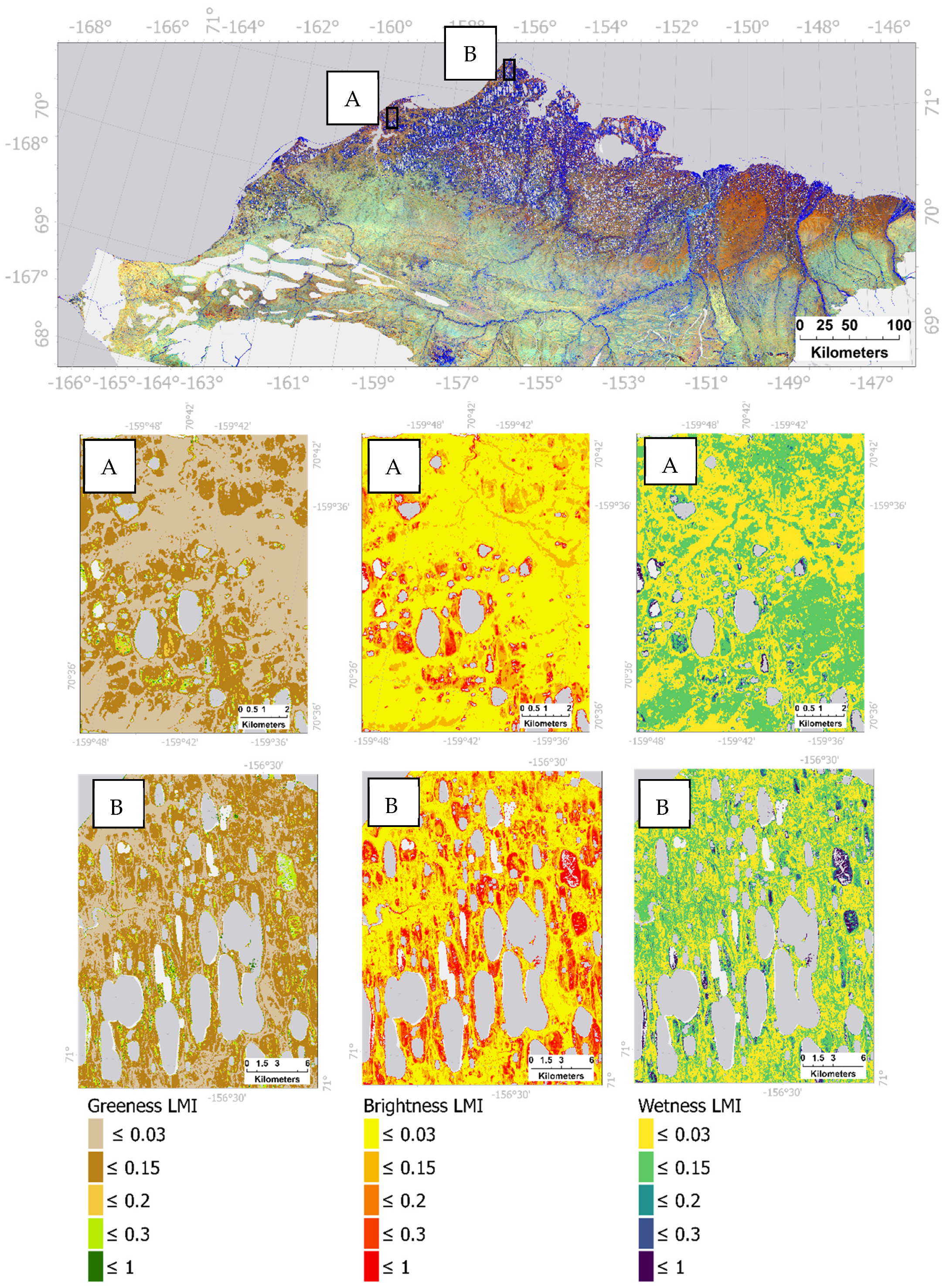
2.3. Local Moran’s I Statistic

We used the local Moran’s I statistic to develop a per-pixel statistical likelihood DLB product based on the TCT from the Landsat-8 mosaic (Figure 4). The Local Moran’s I statistic of spatial association is based on the global Moran’s I and it was first proposed by Anselin [74] as a local indicator of spatial association (LISA) statistic. It is commonly used to detect patterns of spatial clusters. While the global Moran’s I provides a measure for the spatial autocorrelation of a given dataset, the local Moran’s I relates each observation (in the case of satellite imagery, this means each pixel) to its neighbors and it gives an indication of spatial autocorrelation on a local scale. To achieve this, the local Moran’s I estimates and captures the strength of the similarity in x between observations i and j within the neighborhood of i. This statistic is calculated as follows:

$$I_i=\left(\frac{z_i}{\frac{{\sum }_i{z}_i^2}{n}}\right){\displaystyle \sum }_j{w}_{ij}{z}_j$$

(1)

where $z_i=x_i-\overline{x}$ and $w_{ij}$ is the matrix of weights. Equation (1) standardized the value x for observation i. It determined if this value was high or low relative to the regional mean value and subsequently standardized the values of x for j to determine if the neighborhood had high or low values relative to the mean.

In this study, we calculated the local Moran’s I using the MoranLocal function included in the R raster package [75]. The MoranLocal function was applied to the greenness, brightness, and wetness bands of the TCT based on the cloud-free Landsat-8 mosaic. The statistic was calculated using a moving window with a size of 3 × 3 pixels applied to the different bands of the TCT. Different sizes for the moving window were tested with 3 × 3 pixels showing the best results following visual interpretation. High values for the local Moran’s I statistic generally indicate that a given pixel is part of a local cluster, surrounded by pixels showing similarly high or low pixel values. Negative values for the local Moran’s I statistic indicate that the pixel is surrounded by dissimilar values, making it a spatial outlier. Values of 0 represent perfect randomness and no autocorrelation of the pixel and the surrounding values.

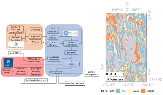
2.4. Remote Sensing-Based Statistical Classification Approach

Our novel remote sensing-based statistical classification approach for mapping DLBs on the North Slope of Alaska combined the results of the local Moran’s I statistic from the TCT data and a landform parameter based on the TPI analysis of the ArcticDEM. We assumed that DLBs had comparably large local Moran’s I values within the basin, caused by DLBs differing from their surrounding areas in greenness, brightness, and wetness and therefore forming clusters with similarly high or low values. was is assumed that areas of negative local Moran’s I values could be excluded from the subsequent analysis, as they represented areas of spatial outliers and were not part of clusters that could signify DLBs. A linear combination of the results from the local Moran’s I statistics of greenness, brightness, and wetness was chosen to determine if the pixels were likely to be located in DLBs. To determine the optimal coefficients for the linear combination of the local Moran’s I results, different coefficients were tested and their results compared with a manually classified point dataset (see Section 2.5). The results of this iterative approach are reported in Section 3.2,

Table 3. Results of the t-test (mean value, p-value, t-value, degrees of freedom (DF)) comparing local Moran’s I (LMI) values for Tasseled Cap (TC) brightness, greenness, and wetness for areas within and outside of the DLBs as classified by Frohn et al. [6].

LMI TCT	Greenness	Brightness	Wetness
DLB Mean	0.08	0.12	0.06
Non-DLB Mean	0.03	0.03	0.03
p-Value	<0.001	<0.001	<0.001
t-value	1591.3	1475.1	553.7
DF	845,5903	756,8750	777,3206

and Figure 7.

The coefficients in Equation (2) were found to be the combination that resulted in the most accurate DLB classification and were used for the DLB dataset presented in this study.

$$\begin{array}{c}{\mathrm{pDLB}}_{\mathrm{raw}}=\mathrm{LMI}\left(\mathrm{brightness}\right)+2\times \mathrm{LMI}\left(\mathrm{greenness}\right)\\ -\mathrm{LMI}\left(\mathrm{wetness}\right)\end{array}$$

(2)

$$\mathrm{pDLB}={\mathrm{pDLB}}_{\mathrm{raw}}\times \mathrm{LP}$$

(3)

Equation (2), including the parameters local Moran’s I (LMI) value for brightness, greenness, and wetness, results in the pDLB_raw value (the probability of a pixel being a DLB), depending solely on the statistics based on the TC values of the Landsat-8 mosaic. Equation (3) combines pDLB_raw with the landform parameter (LP, see Equation (3)) for each pixel based on the landform classification of the ArcticDEM.

This landform parameter (LP) was created to exploit the information contained in a DEM to increase the accuracy of the DLB mapping approach. The LP adjusts the pDLB_raw value depending on the landform classification. As described in Equation (3), the LP can only lower the value of pDLB_raw for certain landforms, not increase the value. Landform types that are assumed to rule out the possibility of DLBs (e.g., smaller mountain tops and ridges missed by the masking approach) were given LP values of 0. For these topographic high points, the pDLB value was set to 0. For each landform type, LP values were chosen by comparing the DEM-based landform classification with satellite imagery and visually assessing the likelihood of DLBs occurring within this landform. Landforms like U-shaped valleys and plains were given the LP value of 1, meaning the pDLB_raw value would not be adjusted. Other landforms were assigned values between 0 and 1, depending on how frequently DLBs occur in these landform types.

2.5. Accuracy Assessment and Calibration

To assess the validity of the remote sensing-based statistical classification approach for classifying DLBs on the North Slope of Alaska, 1500 points were randomly generated using the ArcGIS Create Random Points tool and manually classified in ArcGIS into DLB vs. non-DLB. Of the randomly generated points, 147 points were in excluded or masked areas, resulting in 1353 points available for validation within the study area. These random points were compared to with DLB classification results and formed the basis of our primary accuracy assessment. For the comparison, the pDLB as well as DLB classes (DLB/non-DLB, described in Section 2.7) were extracted using the manually classified points. The manual classification was then compared with both the pDLB values and the DLB classes generated by the approach presented in this study. To complement the random point datasets, we also used several ancillary DLB datasets with localized coverage, published in the past, as a secondary accuracy assessment. The datasets used for this purpose are described in Section 2.2.3. To strengthen the results, a Welch 2-sample t-test, as implemented in R as the t.test function, was used to show the validity of the model selection as well as to corroborate the initial assumption of the suitability of the local Moran’s I and Tasseled Cap approach.

2.6. Quantifying Area of Lakes and Drained Lake Basins

To quantify the area of lakes and DLBs in areas of different surficial geology [56], lakes were extracted from the water-mask dataset used to remove water bodies from the DLB mapping analysis. The water-mask included larger lakes as well as remnant lakes within partially drained basins. To separate lakes from other water bodies included in the mask dataset, the raster data were transformed to polygons, and features such as the ocean, coastal water, and rivers were excluded manually.

2.7. Classifying Drained Lake Basins

From the 1353 random points generated for the accuracy assessment, thresholds for DLB presence/absence classification were derived for subsets of the study area. The dataset was divided into subsets representing the areas of the different surficial geology classes based on [56] present in the study area (see Figure 2). Based on the agreement of the manually classified random points for different subsets, thresholds were determined to separate the pDLB values into DLB/non-DLB classes. Due to the data preparation prior to analysis, the non-DLB class did not include rivers, lakes, and mountainous areas. For each subset representing a unique surficial geology class, the lower threshold was defined as the average of the median value of random points classified as DLB and the median value of random points classified as non-DLB. Values under this lower threshold were classified as non-DLB. Values above the median of random points classified as DLB were assigned to the DLB class. To account for areas where pDLB values might not be clearly separable (see the boxplots in Figure 8), a third class for ambiguous values was created, encompassing values above the lower threshold and under the median of pDLB values classified as DLBs.

3. Results

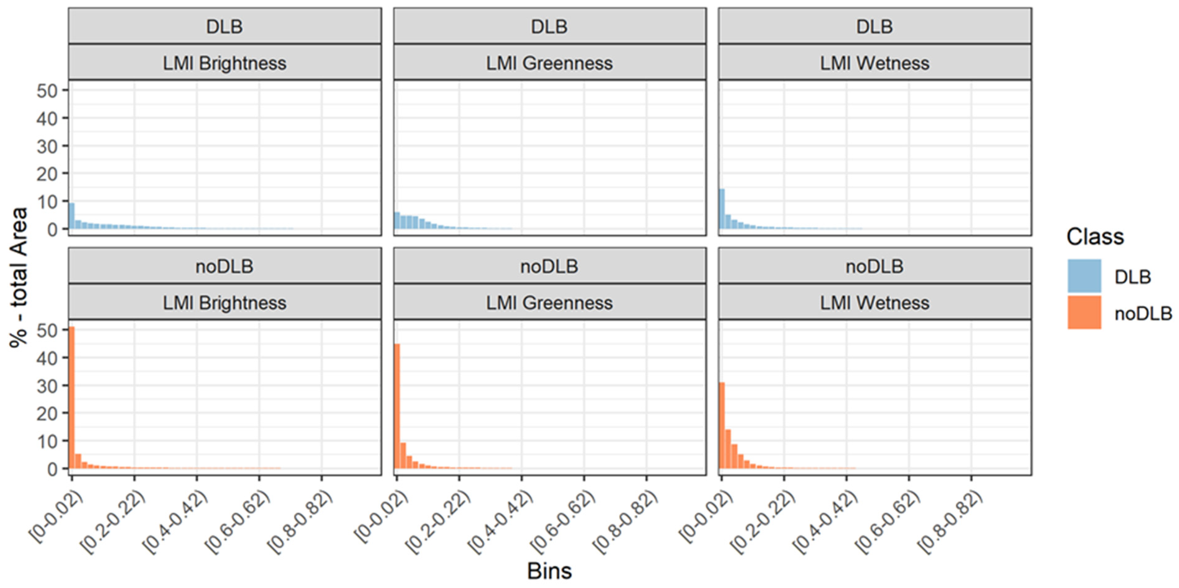
3.1. Local Moran’s I Statistic Based on Tasseled Cap Transformation

The remote sensing-based statistical classification approach using the cloud-free Landsat-8 mosaic for the North Slope of Alaska resulted in a likelihood index for the presence of DLBs. The basis of the DLB likelihood index (pDLB_raw) presented in this study was formed by the statistical analysis of the TCT derived from the cloud-free Landsat-8 mosaic. The local Moran’s I for greenness, brightness, and wetness showed distinct features, suggesting that a combination of all three variables could be suitable for distinguishing between areas likely to be DLBs and those that are unlikely to be DLBs (Figure 5). Figure 5 shows local examples of the local Moran’s I for greenness, brightness, and wetness, with likely areas of DLBs being especially distinct in the greenness and brightness layers. This observation is supported by the histograms shown in Figure 6, which compare the local Moran’s I values for greenness, brightness, and wetness within and outside of DLB areas, based on data from a previously published DLB dataset [63]. For all three parameters (local Moran’s I values for greenness, brightness, and wetness), the areas which were not previously classified as DLBs showed a high percentage of their area to be covered by low values, with >50%, >40%, and >30% of the non-DLB areas showing values between 0 and 0.2 for the local Moran’s I of brightness, greenness, and wetness, respectively. The results of two-sample t-tests supported this observation, showing significant (p-value < 0.001) differences in mean values for the local Moran’s I values for greenness, brightness, and wetness representing areas within and outside of the DLB areas as classified by Frohn et al. [6] (Table 3).

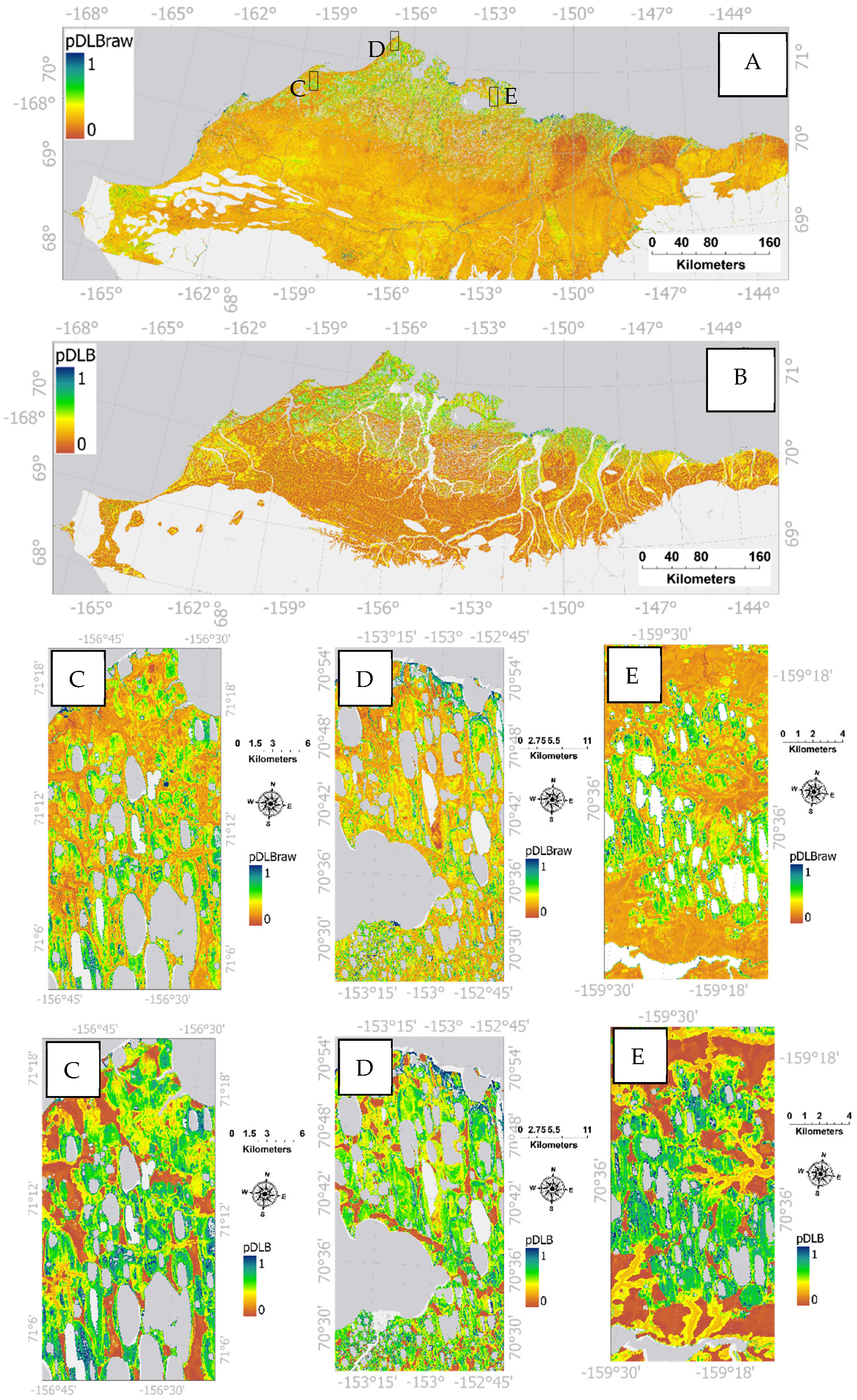
3.2. Defining Drained Lake Basins

The DLB classification presented in this study was based on the equations reported in Section 2.4 (Equations (2) and (3)). Figure 7 shows the comparison of the pDLBraw values to manually classified points. This comparison revealed the ability of the different coefficients to possibly distinguish DLBs. Version 7 was chosen, as it showed the largest differences between pDLB_raw median values for points classified as DLB/non-DLB. The coefficients also exhibited the largest absolute t-value (−21.497, see

Table 4. Coefficients (Coeff.) for local Moran’s I values for brightness, greenness, and wetness (B, G, W) tested during development of the DLB mapping approach, including the results (mean value, p-value, t-value, degree of freedom (DF)) of a two-sample t-test. Version 7 was used in the final equation.

Coefficient Version	Coeff. B	Coeff. G	Coeff. W	pDLBraw Mean within DLB	pDLBraw Mean outside DLB	p-Value	t-Value	DF
1	1	−1	1	0.49	0.17	<0.001	−15.157	298
2	1	−1	−1	0.53	0.23	<0.001	−9.3428	276.67
3	−1	−1	1	0.36	0.18	<0.001	−8.5516	296.02
4	−1	1	−1	0.45	0.16	<0.001	−14.553	292.37
5	1	1	−2	0.41	0.1	<0.001	−16.834	253.5
6	2	2	−1	0.42	0.08	<0.001	−20.691	205.84
7	1	2	−1	0.44	0.1	<0.001	−21.497	246.61

), indicating that this combination of coefficients was the most suitable for distinguishing between DLB and non-DLB areas (Figure 8).

The pDLB_raw parameter, which describes the results of the DLB classification approach before the inclusion of landform information, showed visible delineation of DLBs (see Figure 9). The inclusion of DEM information into the classification approach led to a clearer delineation of DLB features (see Figure 9).

Thresholds for separating the pDLB values into DLB/ambiguous/non-DLB classes were determined separately for areas of different surficial geology (see

Table 5. Areas of lakes and DLBs for different types of surficial geology. DLB areas are based on the final DLB classification. DLB areas includes area directly classified as DLBs; DLB area ranges include areas classified as ambiguous (this includes ground ice content, based on [56]).

Surficial Geology	Lake Area [km2]	DLB Area [km2]	Area Ratio DLB/Lakes	Ranges of DLB Area	Massive Ground Ice Content	pDLB Thresholds
Glaciomarine	1415.40	1049.53	0.74	1049.53–1389.45	10–30%	0.23
Glaciofluvial, old	23.94	12.13	0.5	12.13–59.35	5–30%	0.31
Glacial, young	36.17	-	-	-	10–80%	-
Glacial, old	31.70	0.07	0.002	0.07–0.28	10–80%	0.17
Fluvial, old	1579.88	504.14	0.32	504.14–1069.58	5–30%	0.39
Eolian silt	502.78	35.49	0.07	35.49–12,438.35	30–70%	0.18
Eolian sand	4098.44	2082.32	0.51	2082.32–5410.78	5–10%	0.21
Colluvium upland	45.51	1.02	0.02	1.02–11,177.98	5–10%	0.16
Colluvium basin	13.36	272.66	20.4	272.66–306.83	10–30%	0.28
Coastal plain	4725.8	5599.32	1.18	5599.32–12,162.36	10–30%	0.25

). Initial tests using one threshold for the entire study area did not lead to satisfactory results. Figure 8 shows the pDLB values for manually classified random points with distinct differences among the different surficial geology types. For some types of surficial geology (for example, eolian sand), points manually classified as DLB and non-DLB, respectively, had distinctly different pDLB values. For other surficial geology types, such as colluvium (upland), values for DLB and non-DLB areas had a significant overlap (see Figure 8).

Based on the pDLB values and the manually classified points, the results of this study are the DLB maps presented in Figures 10–13. The DLB maps, based on the pDLB values and the thresholds found through the data presented in Figure 8, were created separately for the areas with different types of surficial geology that are included in Figure 8.

3.3. Accuracy Assessment

A comparison of the manually classified points with the DLB classification results (Figure 8) revealed that of the points manually classified as DLBs, 64.46% were classified as DLB areas by our approach, 31% were classified as ambiguous areas, and 4.54% were classified as non-DLBs by our approach (

Table 6. Error matrix showing the results of the comparison of the DLB classification with the manually classified points.

Reference Datasets		DLB Classification
	DLB	Ambiguous	Non-DLB
DLB	64.46%	31%	4.54%
Non-DLB	4.6%	12.2%	83.2%

). Of the points which were manually classified as non-DLBs, 83.2% were classified as non-DLBs by our approach, 12.2% were classified as ambiguous, and 4.6% were classified as DLBs by our approach (Table 6). These percentages varied greatly among different surficial geology types (see Figure 10, Figure 11 and Figure 12).

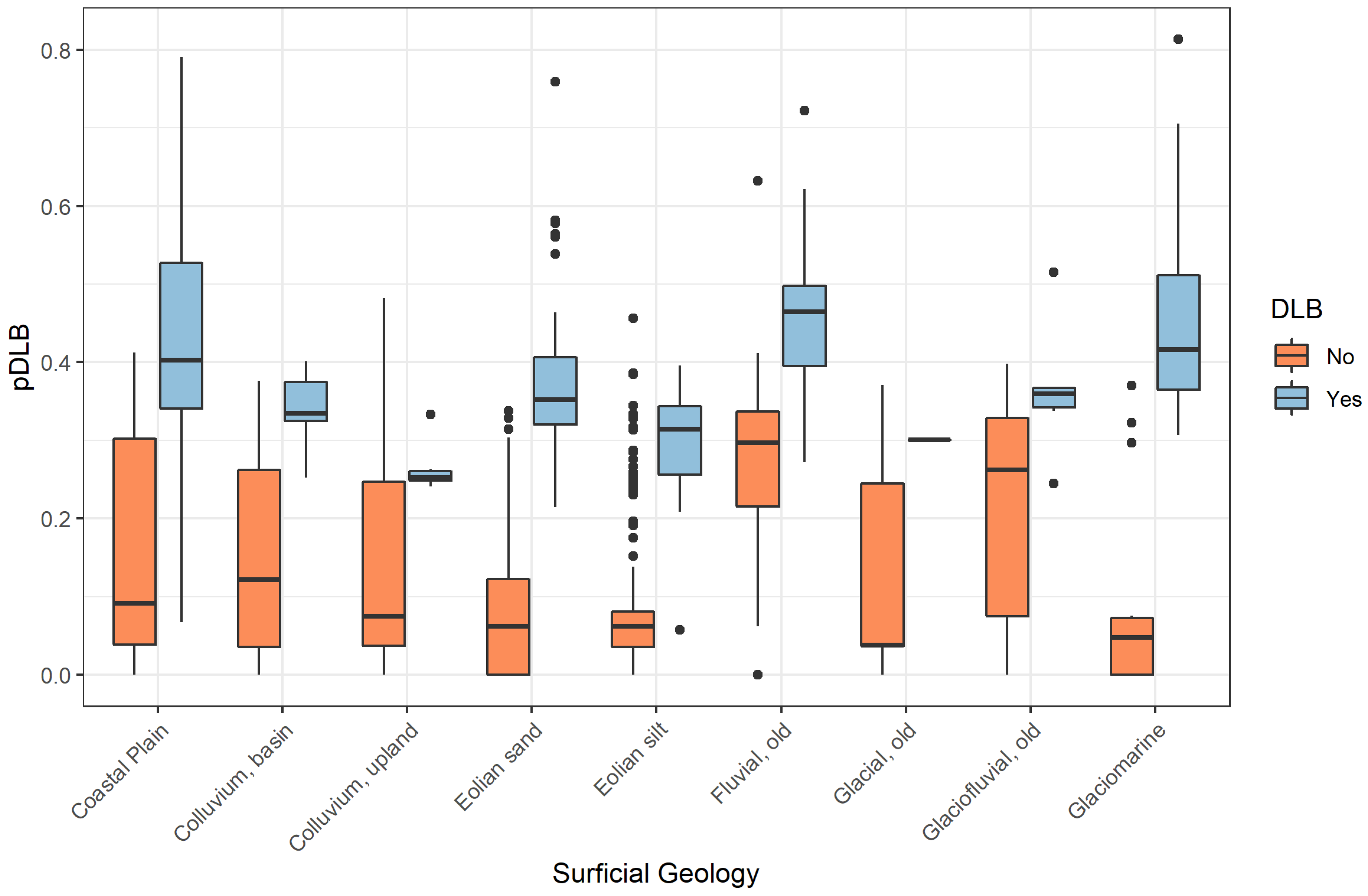
3.4. Areas of Lakes and DLBs for Regions with Different Surficial Geology

The relative area occupied by DLBs is not equally distributed across the subregions of the study area. Areas of different surficial geology have different DLB area extents. Table 4 shows the estimated lake area, based on the water-mask used in this analysis, and the DLB areas for the different surficial geology types present in the study area. The highest areal coverage of both DLBs and lakes was found in areas of the coastal plain and areas of eolian sand. When we considered the ratio of DLB area to lake area, areas described as colluvium basin and the coastal plain had the highest values. Ranges of DLB areas included minimum values based on the extent of the DLB class and the extent of both the DLB and the ambiguous class combined.

4. Discussion

4.1. DLB Data Product

Our approach resulted in a comprehensive DLB classification for the North Slope of Alaska covering >71,000 km², including previously mapped areas [6,11,73], as well as 55% of newly mapped terrain (Figure 13). The classification approach captured the diversity in DLBs prevalent in the study area, including permafrost areas with varying volumetric ground ice content, and in regions with differing tundra vegetation communities. This approach differs from previously published mapping methodologies that relied on DLBs’ similarity to each other, assuming DLBs are similar to each other in spectral values and shape and match a substantial amount of the training data [6,7]. The training data of these previous approaches required significant manual interaction in the classification workflows. Our approach relied on the DLBs demonstrating different characteristics compared with the surrounding areas in greenness, wetness, and brightness and in landform characteristics, as derived from the ArcticDEM. Exploiting this difference in characteristics instead of relying on classification methods based on basins’ similarity to each other in pixel values or shape parameters allowed this approach to be applied to a wide range of environments and DLB types, such as shallower basins, recently drained basins, and basins drained thousands of years ago.

The basis of the classification approach presented in this paper was the results of the local Moran’s I for the three bands of the Tasseled Cap Transformation (brightness, greenness, and wetness). This was shown to be a suitable approach for extracting DLB areas from Landsat imagery, with significant differences (p-value < 0.001) between DLB and non-DLB areas (as classified by Frohn et al. [6]). The results of the t-test strengthened the initial observations based on visual interpretation of the TCT (Figure 9), which suggested that the DLBs can be identified by using the TCT. The local Moran’s I was calculated by using a set moving window size of 3 × 3 pixels, translating to an area of 90 m × 90 m (taking into account the 30 m Landsat-8 pixel size). Larger window sizes are likely to miss smaller DLBs, as well as drained areas of partially drained basins. While smaller than 90 m × 90 m window sizes might be suitable for DLB mapping utilizing higher resolution satellite imagery, with the given resolution of Landsat-8 (30 m), this would not be a valid approach.

Our approach relies in part on a landform classification [67] separating different relief types which can be associated with DLB features (e.g., valleys, slopes) or that can be assumed not to be DLBs (e.g., ridges, summits, streams, and drainages). In order to include the landform information into the DLB classification approach, each landform was assigned an LP value, adjusting the pDLB_raw value. It is important to note that this adjustment was designed to lower the pDLB_raw value for areas with landforms unlikely to be DLBs and had no possibility of increasing the pDLB_raw value. It therefore could not be higher than the value resulting from Equation (3), based on the Tasseled Cap local Moran’s I values. Specific LP values for the different landform classes were derived by visual comparison of the landform classification and previously published DLB data (specifically from Frohn et al. [6]; see Figure 3). Before possibly applying this method to a different or a larger study area, revisiting or adjusting this parameter to suit the specific study region is prudent. However, the area of interest in this study covers a wide range of Arctic tundra landscape types, ranging from coastal areas to the foothills of the Brooks Range. It can therefore be assumed that the LP values used in this study are somewhat robust. The TPI has been previously used in studies in combination with multispectral imagery [76,77,78]; however, the combination of a Landsat-8 based TCT with TPI inferred landform classes for landform mapping on a large scale is, to the best of our knowledge, a novel approach. While this landform classification approach was not originally designed for Arctic or cold-region environments, it proved to be a valuable tool for excluding certain areas from the DLB mapping approach, as well as showing the increased likelihood of other areas being DLBs. However, when DLBs that had low elevation differences from the surrounding landscape (e.g., low relief DLBs) or that had especially steep rims, low pDLB values were resolved for DLBs in some parts of the study area, resulting in misclassification and thus exclusion from the DLB dataset. Low-relief DLBs are often missed by the landform classification used in this approach [67,69] and are instead classified as part of plains and included in the ambiguous category. We argue that the use of DEMs with higher vertical resolution and accuracy, such as provided, for example, by airborne Light Detection and Ranging (LiDAR), could overcome the challenge of misclassifying very shallow DLBs. However, for a pan-Arctic approach, this type of data is not available. In addition, the TPI classification is sensitive to the resolution of the input DEM data. The ArcticDEM is available in 2-m resolution (as well as versions with reduced spatial resolutions of 10 m, 32 m, 100 m, 500 m, and 1 km). To reduce the influence of potential noise within the DEM data, as well as to cut down the computing time needed for applying this method to large study areas, the 10-m resolution version was chosen for our approach. It was assumed that this resolution would be sufficient to adequately represent DLB features. However, if this method would be applied, for example, to study spatial differences within basins, remnant lake features, or other features with small scale variability, a higher-resolution DEM might be more suitable.

In this study, pixels classified as DLBs were limited to areas which had completely drained, meaning that remnant lakes and other areas with open water within DLB features were not included in the results and were missing from the estimation of DLB area presented here. This should be taken into consideration when comparing the numbers presented here with already published or future estimates of DLB area on a pan-Arctic scale. While our study offers a comprehensive and novel approach to the classification of DLBs, the classification method cannot directly distinguish separate parts of overlapping or joined DLB features. Multi-generation separation of individual sub-basins from such coalesced DLBs would require manual post-processing of the presented dataset. Overlapping DLB features with often more than two connected or overlapping basins are common within the study area [6,10]. As such, in other regions, multiple overlapping basin generations are also common. For example, on the northern Seward Peninsula, up to seven overlapping generations of basins have been identified [10]. In the Lena Delta, the Yedoma uplands contain a large number of nested DLBs that form large complexes of deeply incised drained lake basins [16]. In several regions of northeastern Siberia, such as the Kolyma lowlands, overlapping DLBs dominate the landscape entirely, indicating massive degradation of permafrost by lake formation and drainage in the past [13]. Hence, the limitation in our approach to identify individual DLB features may result in an underestimate of the number of individual DLB features. However, our primary focus was on estimating the total areal coverage of DLBs, and a count of separate DLB features was not attempted here.

In addition, individual DLBs are not homogeneous features [7,42] and often show spatial heterogeneity within one basin, particularly as the basin ages [42]. These spatial differences include differences in surface moisture, vegetation patterns, and the presence or absence of remnant water bodies caused by partial drainage and complex drainage histories [11,23,25,27]. The spatial heterogeneity with DLBs led to differences in pDLB values within single basins and added to the difficulty of delineating basins based on the results presented in this study. Further separation of identified basin areas could rely on spectral characteristics associated with successional dynamics post-drainage [10,43] and potentially morphometric object-based characteristics [7].

The classification of our results into the DLB/ambiguous/non-DLB classes allowed for a better quantification of DLB areas compared with the pDLB results. Comparing the results with existing datasets as well as with manually classified random points showed the high potential of the approach for scaling to larger domains. Figure 8 shows the importance of treating areas with different surficial geology separately for classification. Manually classified random points did not allow for a clear separation of DLB and non-DLB areas for all areas with different surficial geology. The ambiguous class encompassed values that cannot be assigned to the other classes with statistical confidence. This allowed for a conservative estimate of DLB area (only including the DLB class) and a more encompassing estimate, including both the DLB and ambiguous classes, indicating the potential maximum range in DLB coverage of a landscape cover. Thresholds used for the classification were derived separately for the areas with different surficial geology (Table 5) and varied between a pDLB of 0.16 and 0.39. These large differences in thresholds further highlight the importance of treating areas with different surficial conditions separately in this process. For surficial geology classes where pDLB values were not clearly separated between DLB and non-DLB, the potential for misclassification of DLB as non-DLB areas (or the opposite) became more likely. For these areas, the ambiguous class naturally becomes of greater importance, as it will limit misclassified areas and, instead, clearly indicates the underlying uncertainty involved for these specific regions. Potential users of the dataset could decide on an application-specific basis if they wish to use the conservative estimate excluding the ambiguous class, or to utilize all classes, potentially including a larger area of non-DLBs which were misclassified.

Additional sources of uncertainty include the wide temporal range of the Landsat input data due to the requirement of creating a cloud-free mosaic, resulting in the potential for missing recent lake drainage events. A further potential source of error is the data gaps in the Arctic DEM, which may be relevant in some Arctic regions more affected by poor imaging conditions.

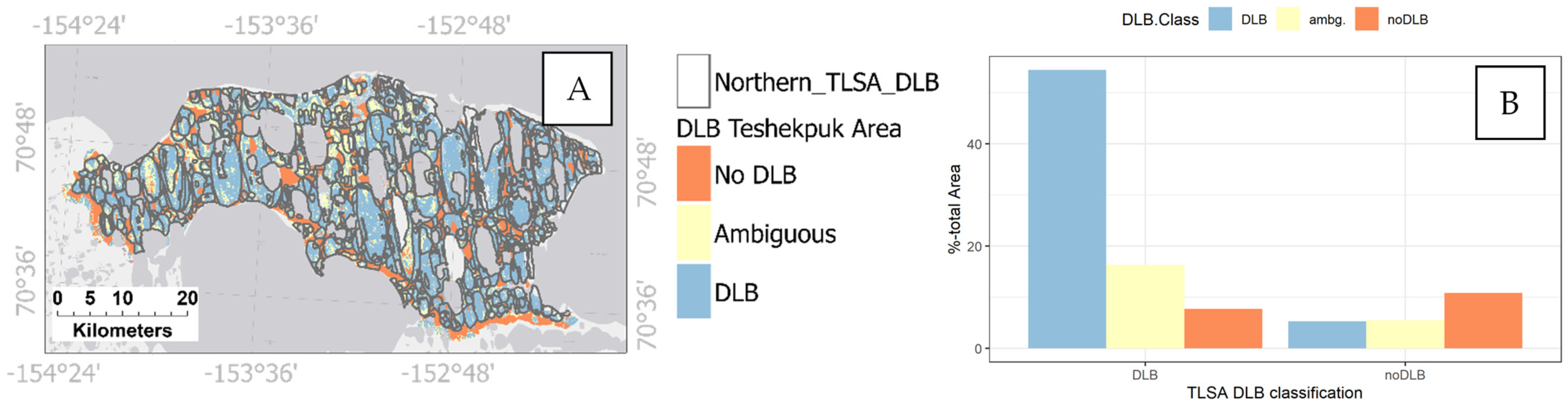
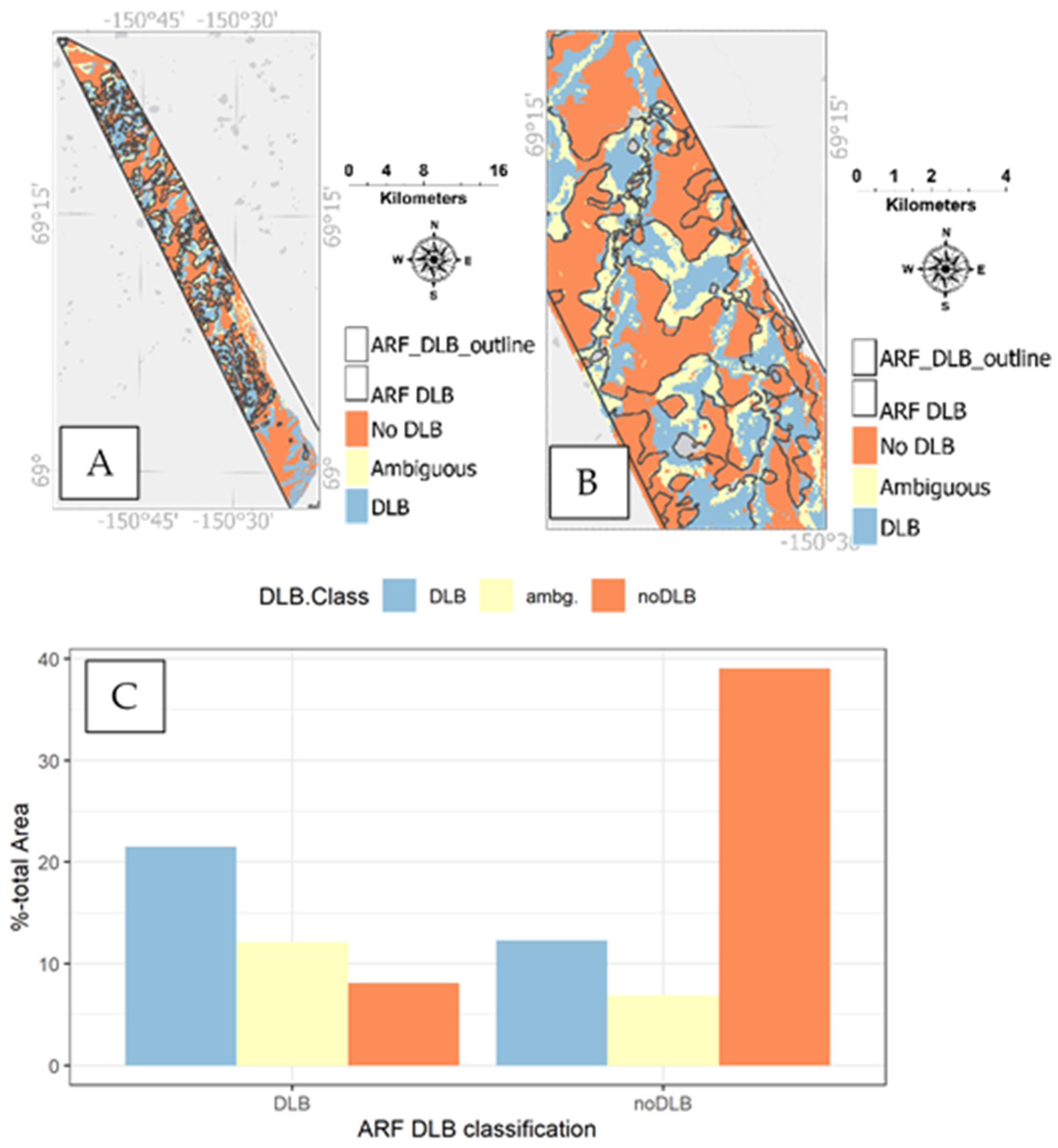
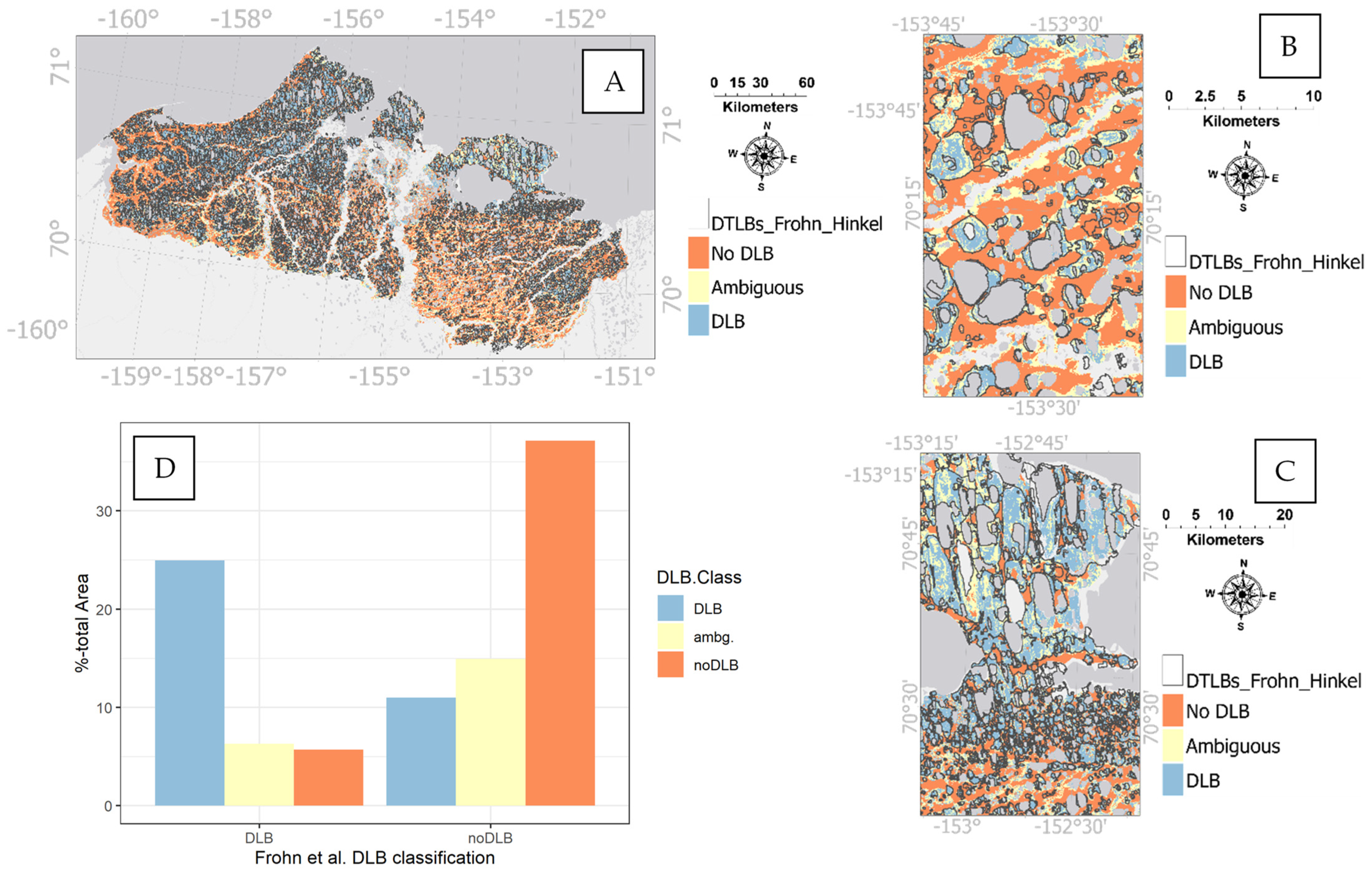
4.2. Comparison of DLB Classification with Previously Published Datasets

A comparison of the DLB classification results with existing DLB datasets for parts of the study area was made as a secondary accuracy assessment (Figure 10, Figure 11 and Figure 12). A comparison of the DLB classification results to the DLB dataset presented in Frohn et al. [6] is shown in Figure 9 and indicates an agreement of 25% of the area classified as DLBs and >36% classified as non-DLB sin both datasets. Approximately 21% of the area was classified as ambiguous in our approach, with most of this area being classified as non-DLB area in the previously published dataset. For 15% of the area, our classification results and the Frohn dataset disagreed, with a majority of these areas being classified as DLBs in our approach and as non-DLBs by Frohn et al. [6]. A comparison of our results with the dataset presented by Jones et al. [11], shown in Figure 11, reveals good general agreement, with >53% of the total area being classified as DLBs in both datasets and 11% of the area being classified as non-DLBs by both datasets; however 7% of the area was classified as DLBs in the previously published dataset but as non-DLBs by our approach. A comparison of our results with the DLB data published in Jones et al. [73] (Figure 12) shows that a large portion of the area was classified as non-DLB in both datasets (39%) and 21% of the area was classified as DLBs in both datasets; however, 12% of the area was classified as non-DLBs in the previously published dataset but as DLBs by our approach.

4.3. Lakes and Drained Lake Basins on the North Slope of Alaska

Lakes and DLBs are common features in the Arctic landscape of the North Slope of Alaska. Previous studies have described the distribution of lakes and DLBs for different terrain types in the region, but a wall-to-wall map of the North Slope was lacking [6,22,79,80,81]. By quantifying the proportion of lakes and DLBs in particular areas (i.e., by differing surficial geologies) and across the entirety of the North Slope, for the first time, this study provides critical information as to the rate of past landscape changes and a lens on the variability in landscape dynamics operating over the course of millennia. For example, general geology types that contain generally ice-rich permafrost deposits have a DLB:lake ratio that exceeds 0.7. In terrain with generally moderate to low permafrost ground ice content, the DLB:lake ratio ranges from 0.3 to 0.5, while in terrain with generally ice-poor permafrost deposits, the DLB:lake ratio is essentially zero. Thus, identifying the ratio of DLBs to lakes in regions with varying permafrost ground ice conditions provides a better understanding regarding the dynamics of surficial processes and the underlying landscape characteristics. Mapping the variability in permafrost ground ice conditions is inherently challenging (e.g., [9]); therefore, the observations provided by our remote-sensing based approach in this study could be used to better inform regional and pan-Arctic permafrost region mapping efforts.

4.4. Potential Applications and Upscaling of the Results

By using widely available input data, such as Landsat imagery, the ArcticDEM, and ancillary geospatial datasets that describe surface geology conditions, our classification approach appears to be useful for mapping DLBs in lowland permafrost regions across the Arctic. This makes the approach a valuable tool for a wide range of applications which require reliable DLB maps as inputs for their analysis. Possible applications for this dataset could be the upscaling of relevant field measurements in connection with the presence or absence of DLBs, upscaling basin ages based on radiocarbon dating results to achieve an estimate of basin age distribution across larger study regions [10,42,43], and habitat mapping for lowland permafrost regions in the Arctic. The dataset also has the potential to act as input data in future modeling approaches, including hydrological models, snow modeling, and permafrost models. The wide availability of Landsat-8 imagery and the generally good coverage over Arctic areas allows for potentially applying this approach on a circumpolar or pan-Arctic scale. While the ArcticDEM is available on a pan-Arctic level, it currently has gaps, especially over parts of Siberia. Regions with poor ArcticDEM coverage might require an alternate or supplemental DEM dataset, filling the gaps or extending the study area southward (as the ArcticDEM is limited to areas above 60° N) to apply this classification approach. A pan-Arctic DLB product would substantially help with efforts concerning quantification of soil carbon, particularly permafrost soil carbon affected by prior lake thermokarst [81,82,83,84,85]. Further, understanding DLBs’ distribution and ages will help in quantifying quaternary lake formation and persistence dynamics, which is directly relevant for determining lakes’ history as well as lakes’ methane dynamic [86]. A wide-spanning and especially a pan-Arctic DLB product will also help scaling high-latitude wetland methane emissions during the Holocene [86] and more generally help place current lake drainage dynamics in a wider spatial and temporal perspective [11,24,26,27].

5. Conclusions

The approach to mapping areas of DLBs in permafrost environments presented in this study was shown to be effective over areas with different Quaternary histories and over the large environmental and climatic gradient that is present on the North Slope of Alaska. The area included in this study covers >71,000 km², including a >39,000 km² area not previously covered in existing DLB datasets. We showed the importance of treating areas with different surficial geology separately in DLB classification schemes due to DLBs in different areas having distinct characteristics and requiring different classification thresholds. The results were shown to be consistent with prior existing regional DLB datasets (up to 87% agreement, depending on the dataset) and show high agreement with manually classified random points (64.4–95.5% for DLB and 83.2–95.4% for non-DLB areas). This methodology has the potential to map DLBs on a pan-Arctic scale, providing a comprehensive workflow for DLB mapping where suitable Landsat imagery, ArcticDEM data, and information on variability in surficial geology exist. Comprehensive mapping of DLB areas across the circumpolar permafrost landscape would allow for future utilization of these data in pan-Arctic models and greatly further our understanding of DLBs in the context of permafrost landscapes. This approach relies on freely available multispectral and DEM datasets, highlighting the importance of freely available and accessible remote sensing datasets to the research community.

References

1. Lara, M.J.; Nitze, I.; Grosse, G.; Martin, P.; McGuire, A.D. Reduced Arctic Tundra Productivity Linked with Landform and Climate Change Interactions. Sci. Rep. 2018, 8, 2345. [Google Scholar] [CrossRef] [PubMed]
2. Lantz, T.C. Vegetation Succession and Environmental Conditions Following Catastrophic Lake Drainage in Old Crow Flats, Yukon. Arctic 2017, 70, 177–189. [Google Scholar] [CrossRef]
3. Hashemi, J.; Zona, D.; Arndt, K.A.; Kalhori, A.; Oechel, W.C. Seasonality Buffers Carbon Budget Variability across Heterogeneous Landscapes in Alaskan Arctic Tundra. Environ. Res. Lett. 2021, 16, 35008. [Google Scholar] [CrossRef]
4. Arp, C.D.; Jones, B.M.; Hinkel, K.M.; Kane, D.L.; Whitman, M.S.; Kemnitz, R. Recurring Outburst Floods from Drained Lakes: An Emerging Arctic Hazard. Front. Ecol. Environ. 2020, 18, 384–390. [Google Scholar] [CrossRef]
5. Grosse, G.; Jones, B.M.; Arp, C.D. Thermokarst lakes, drainage, and drained basins. In Treatise on Geomorphology; Shroder, J.F., Ed.; Elsevier: Amsterdam, The Netherlands, 2013; Volume 8, pp. 325–353. [Google Scholar]
6. Frohn, R.C.; Hinkel, K.M.; Eisner, W.R. Satellite Remote Sensing Classification of Thaw Lakes and Drained Thaw Lake Basins on the North Slope of Alaska. Remote Sens. Environ. 2005, 97, 116–126. [Google Scholar] [CrossRef]
7. Hinkel, K.M.; Frohn, R.C.; Nelson, F.E.; Eisner, W.R.; Beck, R.A. Morphometric and Spatial Analysis of Thaw Lakes and Drained Thaw Lake Basins in the Western Arctic Coastal Plain, Alaska. Permafr. Periglac. Process. 2005, 16, 327–341. [Google Scholar] [CrossRef]
8. Jorgenson, M.T.; Shur, Y. Evolution of Lakes and Basins in Northern Alaska and Discussion of the Thaw Lake Cycle. J. Geophys. Res. Earth Surf. 2007, 112, F02S17. [Google Scholar] [CrossRef]
9. Kanevskiy, M.; Shur, Y.; Jorgenson, M.T.; Ping, C.L.; Michaelson, G.J.; Fortier, D.; Stephani, E.; Dillon, M.; Tumskoy, V. Ground Ice in the Upper Permafrost of the Beaufort Sea Coast of Alaska. Cold Reg. Sci. Technol. 2013, 85, 56–70. [Google Scholar] [CrossRef]
10. Jones, M.C.; Grosse, G.; Jones, B.M.; Walter Anthony, K. Peat Accumulation in Drained Thermokarst Lake Basins in Continuous, Ice-Rich Permafrost, Northern Seward Peninsula, Alaska. J. Geophys. Res. Biogeosci. 2012, 117. [Google Scholar] [CrossRef]
11. Jones, B.M.; Arp, C.D. Observing a Catastrophic Thermokarst Lake Drainage in Northern Alaska. Permafr. Periglac. Process. 2015, 26, 119–128. [Google Scholar] [CrossRef]
12. Farquharson, L.M.; Mann, D.H.; Grosse, G.; Jones, B.M.; Romanovsky, V.E. Spatial Distribution of Thermokarst Terrain in Arctic Alaska. Geomorphology 2016, 273, 116–133. [Google Scholar] [CrossRef] [Green Version]
13. Veremeeva, A.; Nitze, I.; Günther, F.; Grosse, G.; Rivkina, E. Geomorphological and Climatic Drivers of Thermokarst Lake Area Increase Trend (1999–2018) in the Kolyma Lowland Yedoma Region, North-eastern Siberia. Remote Sens. 2021, 13, 178. [Google Scholar] [CrossRef]
14. Hughes-Allen, L.; Bouchard, F.; Laurion, I.; Séjourné, A.; Marlin, C.; Hatté, C.; Costard, F.; Fedorov, A.; Desyatkin, A. Seasonal Patterns in Greenhouse Gas Emissions from Thermokarst Lakes in Central Yakutia (Eastern Siberia). Limnol. Oceanogr. 2021, 66, S98–S116. [Google Scholar] [CrossRef]
15. Serikova, S.; Pokrovsky, O.S.; Laudon, H.; Krickov, I.V.; Lim, A.G.; Manasypov, R.M.; Karlsson, J. High Carbon Emissions from Thermokarst Lakes of Western Siberia. Nat. Commun. 2019, 10, 1552. [Google Scholar] [CrossRef] [PubMed] [Green Version]
16. Morgenstern, A.; Grosse, G.; Günther, F.; Fedorova, I.; Schirrmeister, L. Spatial Analyses of Thermokarst Lakes and Basins in Yedoma Landscapes of the Lena Delta. Cryosphere 2011, 5, 849–867. [Google Scholar] [CrossRef] [Green Version]
17. Sibley, P.K.; White, D.M.; Cott, P.A.; Lilly, M.R. Introduction to Water Use from Arctic Lakes: Identification, Impacts, and Decision Support. J. Am. Water Resour. Assoc. 2008, 44, 273–275. [Google Scholar] [CrossRef] [Green Version]
18. Jones, B.M.; Arp, C.D.; Hinkel, K.M.; Beck, R.A.; Schmutz, J.A.; Winston, B. Arctic Lake Physical Processes and Regimes with Implications for Winter Water Availability and Management in the National Petroleum Reserve Alaska. Environ. Manag. 2009, 43, 1071–1084. [Google Scholar] [CrossRef]
19. Alessa, L.; Kliskey, A.; Lammers, R.; Arp, C.; White, D.; Hinzman, L.; Busey, R. The Arctic Water Resource Vulnerability Index: An Integrated Assessment Tool for Community Resilience and Vulnerability with Respect to Freshwater. Environ. Manag. 2008, 42, 523–541. [Google Scholar] [CrossRef] [PubMed]
20. Derksen, D.V.; Eldridge, W.D.; Weller, M.W. Habitat Ecology of Pacific Black Brant and Other Geese Moulting near Teshekpuk Lake, Alaska. Wildfowl 1982, 33, 39–57. [Google Scholar]
21. Arp, C.D.; Jones, B.M.; Schmutz, J.A.; Urban, F.E.; Jorgenson, M.T. Two Mechanisms of Aquatic and Terrestrial Habitat Change along an Alaskan Arctic Coastline. Polar Biol. 2010, 33, 1629–1640. [Google Scholar] [CrossRef] [Green Version]
22. Jones, B.M.; Grosse, G.; Arp, C.D.; Jones, M.C.; Walter Anthony, K.M.; Romanovsky, V.E. Modern Thermokarst Lake Dynamics in the Continuous Permafrost Zone, Northern Seward Peninsula, Alaska. J. Geophys. Res. Biogeosci. 2011, 116, G00M03. [Google Scholar] [CrossRef]
23. Hinkel, K.M.; Jones, B.M.; Eisner, W.R.; Cuomo, C.J.; Beck, R.A.; Frohn, R. Methods to Assess Natural and Anthropogenic Thaw Lake Drainage on the Western Arctic Coastal Plain of Northern Alaska. J. Geophys. Res. Earth Surf. 2007, 112, F02S16. [Google Scholar] [CrossRef] [Green Version]
24. Marsh, P.; Russell, M.; Pohl, S.; Haywood, H.; Onclin, C. Changes in Thaw Lake Drainage in the Western Canadian Arctic from 1950 to 2000; John Wiley & Sons, Ltd.: Hoboken, NJ, USA, 2009; Volume 23, pp. 145–158. [Google Scholar]
25. Jones, B.M.; Arp, C.D.; Grosse, G.; Nitze, I.; Lara, M.J.; Whitman, M.S.; Farquharson, L.M.; Kanevskiy, M.; Parsekian, A.D.; Breen, A.L.; et al. Identifying Historical and Future Potential Lake Drainage Events on the Western Arctic Coastal Plain of Alaska. Permafr. Periglac. Process. 2020, 31, 110–127. [Google Scholar] [CrossRef] [PubMed] [Green Version]
26. Nitze, I.; Grosse, G.; Jones, B.M.; Romanovsky, V.E.; Boike, J. Remote Sensing Quantifies Widespread Abundance of Permafrost Region Disturbances across the Arctic and Subarctic. Nat. Commun. 2018, 9, 5423. [Google Scholar] [CrossRef] [PubMed]
27. Nitze, I.; Cooley, S.W.; Duguay, C.R.; Jones, B.M.; Grosse, G. The Catastrophic Thermokarst Lake Drainage Events of 2018 in Northwestern Alaska: Fast-Forward into the Future. Cryosphere 2020, 14, 4279–4297. [Google Scholar] [CrossRef]
28. Van Der Kolk, H.J.; Heijmans, M.M.P.D.; Van Huissteden, J.; Pullens, J.W.M.; Berendse, F. Potential Arctic Tundra Vegetation Shifts in Response to Changing Temperature, Precipitation and Permafrost Thaw. Biogeosciences 2016, 13, 6229–6245. [Google Scholar] [CrossRef] [Green Version]
29. Sellmann, P.V.; Brown, J.; Lewellen, R.I.; McKim, H.; Merry, C. The Classification and Geomorphic Implications of Thaw Lakes on the Arctic Coastal Plain, Alaska; US Department of Defense, Department of the Army, Corps of Engineers, Cold Regions Research and Engineering Laboratory: Hanover, Germany; New Hampshire, NE, USA, 1975; Volume 344. [Google Scholar]
30. Wang, J.; Sheng, Y.; Hinkel, K.M.; Lyons, E.A. Drained Thaw Lake Basin Recovery on the Western Arctic Coastal Plain of Alaska Using High-Resolution Digital Elevation Models and Remote Sensing Imagery. Remote Sens. Environ. 2012, 119, 325–336. [Google Scholar] [CrossRef]
31. Labrecque, S.; Lacelle, D.; Duguay, C.R.; Lauriol, B.; Hawkings, J. Contemporary (1951–2001) Evolution of Lakes in the Old Crow Basin, Northern Yukon, Canada: Remote Sensing, Numerical Modeling, and Stable Isotope Analysis. Arctic 2009, 62, 225–238. [Google Scholar] [CrossRef] [Green Version]
32. Qin, Y.; Lu, P.; Li, Z. Semi-Automated Detection of Thaw Lakes in Permafrost Areas in Qinghai-Tibet Plateau from Sentinel-2 Images Using Markov Random Field. In Proceedings of the IGARSS 2019—2019 IEEE International Geoscience and Remote Sensing Symposium; Institute of Electrical and Electronics Engineers (IEEE), Yokohama, Japan, 28 July–2 August 2019; pp. 4036–4039. [Google Scholar]
33. Simpson, C.E.; Arp, C.D.; Sheng, Y.; Carroll, M.L.; Jones, B.M.; Smith, L.C. Landsat-Derived Bathymetry of Lakes on the Arctic Coastal Plain of Northern Alaska. Earth Syst. Sci. Data 2021, 13, 1135–1150. [Google Scholar] [CrossRef]
34. Bartsch, A.; Pointner, G.; Leibman, M.O.; Dvornikov, Y.A.; Khomutov, A.; Trofaier, A.M. Circumpolar Mapping of Ground-Fast Lake Ice. Front. Earth Sci. 2017, 5, 12. [Google Scholar] [CrossRef] [Green Version]
35. Al-Roubaiey, A.; Sheltami, T.; Mahmoud, A.; Shakshuki, E.; Mouftah, H. AACK: Adaptive Acknowledgment Intrusion Detection for MANET with Node Detection Enhancement. In Proceedings of the 24th IEEE International Conference on Advanced Information Networking and Applications, Perth, Australia, 20–23 April 2010; Volume 17, pp. 634–640. [Google Scholar] [CrossRef]
36. Surdu, C.M.; Duguay, C.R.; Pour, H.K.; Brown, L.C. Ice Freeze-up and Break-up Detection of Shallow Lakes in Northern Alaska with Spaceborne SAR. Remote Sens. 2015, 7, 6133–6159. [Google Scholar] [CrossRef] [Green Version]
37. Engram, M.; Anthony, K.W.; Meyer, F.J.; Grosse, G. Synthetic Aperture Radar (SAR) Backscatter Response from Methane Ebullition Bubbles Trapped by Thermokarst Lake Ice. Can. J. Remote Sens. 2013, 38, 667–682. [Google Scholar] [CrossRef]
38. Zhang, S.; Pavelsky, T.M. Remote Sensing of Lake Ice Phenology across a Range of Lakes Sizes, ME, USA. Remote Sens. 2019, 11, 1718. [Google Scholar] [CrossRef] [Green Version]
39. Engram, M.; Arp, C.D.; Jones, B.M.; Ajadi, O.A.; Meyer, F.J. Analyzing Floating and Bedfast Lake Ice Regimes across Arctic Alaska Using 25 years of Space-Borne SAR Imagery. Remote Sens. Environ. 2018, 209, 660–676. [Google Scholar] [CrossRef]
40. Pointner, G.; Bartsch, A.; Dvornikov, Y.; Kouraev, A. Mapping Potential Signs of Gas Emissions in Ice of Lake Neyto, Yamal, Russia Using Synthetic Aperture Radar and Multispectral Remote Sensing Data. Cryosphere 2021, 15, 1907–1929. [Google Scholar] [CrossRef]
41. Nitze, I.; Grosse, G.; Jones, B.M.; Arp, C.D.; Ulrich, M.; Fedorov, A.; Veremeeva, A. Landsat-Based Trend Analysis of Lake Dynamics across Northern Permafrost Regions. Remote Sens. 2017, 9, 640. [Google Scholar] [CrossRef] [Green Version]
42. Hinkel, K.M.; Eisner, W.R.; Bockheim, J.G.; Nelson, F.E.; Peterson, K.M.; Dai, X. Spatial Extent, Age, and Carbon Stocks in Drained Thaw Lake Basins on the Barrow Peninsula, Alaska. Arctic Antarct. Alp. Res. 2003, 35, 291–300. [Google Scholar] [CrossRef] [Green Version]
43. Regmi, P.; Grosse, G.; Jones, M.C.; Jones, B.M.; Anthony, K.W. Characterizing Post-Drainage Succession in Thermokarst Lake Basins on the Seward Peninsula, Alaska with TerraSAR-X Backscatter and Landsat-Based NDVI Data. Remote Sens. 2012, 4, 3741–3765. [Google Scholar] [CrossRef] [Green Version]
44. Marcus, M.G.; Wahrhaftig, C. Physiographic Divisions of Alaska. Geogr. Rev. 1967, 57, 581. [Google Scholar] [CrossRef]
45. Osterkamp, T.E.; Payne, M.W. Estimates of Permafrost Thickness from Well Logs in Northern Alaska. Cold Reg. Sci. Technol. 1981, 5, 13–27. [Google Scholar] [CrossRef]
46. Van Everdingen, R.O.; Terminology Working Group. Multi-Language Glossary of Permafrost and Related Ground-Ice Terms in Chinese, English, French, German, Icelandic, Italian, Norwegian, Polish, Romanian, Russian, Spanish, and Swedish; International Permafrost Association: Calgary, Alberta, 1998. [Google Scholar]
47. Hinkel, K.M.; Nelson, F.E. Spatial and Temporal Patterns of Active Layer Thickness at Circumpolar Active Layer Monitoring (CALM) Sites in Northern Alaska, 1995–2000. J. Geophys. Res. Atmos. 2003, 108, 8168. [Google Scholar] [CrossRef]
48. Walker, D.A.; Jia, G.J.; Epstein, H.E.; Raynolds, M.K.; Chapin, I.S.; Copass, C.; Hinzman, L.D.; Knudson, J.A.; Maier, H.A.; Michaelson, G.J.; et al. Vegetation-Soil-Thaw-Depth Relationships along a Low-Arctic Bioclimate Gradient, Alaska: Synthesis of Information from the ATLAS Studies. Permafr. Periglac. Process. 2003, 14, 103–123. [Google Scholar] [CrossRef]
49. Walker, D.A.; Reynolds, M.K.; Daniëls, F.J.A.; Einarsson, E.; Elvebakk, A.; Gould, W.A.; Katenin, A.E.; Kholod, S.S.; Markon, C.J.; Melnikov, E.S.; et al. The Circumpolar Arctic Vegetation Map. J. Veg. Sci. 2005, 16, 267–282. [Google Scholar] [CrossRef]
50. Walker, D.A.; Kuss, P.; Epstein, H.E.; Kade, A.N.; Vonlanthen, C.M.; Raynolds, M.K.; Daniëls, F.J.A. Vegetation of Zonal Patterned-Ground Ecosystems along the North America Arctic Bioclimate Gradient. Appl. Veg. Sci. 2011, 14, 440–463. [Google Scholar] [CrossRef]
51. Gorelick, N.; Hancher, M.; Dixon, M.; Ilyushchenko, S.; Thau, D.; Moore, R. Google Earth Engine: Planetary-Scale Geospatial Analysis for Everyone. Remote Sens. Environ. 2017, 202, 18–27. [Google Scholar] [CrossRef]
52. Li, H.; Wan, W.; Fang, Y.; Zhu, S.; Chen, X.; Liu, B.; Hong, Y. A Google Earth Engine-Enabled Software for Efficiently Generating High-Quality User-Ready Landsat Mosaic Images. Environ. Model. Softw. 2019, 112, 16–22. [Google Scholar] [CrossRef]
53. Johansen, K.; Phinn, S.; Taylor, M. Mapping Woody Vegetation Clearing in Queensland, Australia from Landsat Imagery Using the Google Earth Engine. Remote Sens. Appl. Soc. Environ. 2015, 1, 36–49. [Google Scholar] [CrossRef]
54. Jin, Y.; Liu, X.; Yao, J.; Zhang, X.; Zhang, H. Mapping the Annual Dynamics of Cultivated Land in Typical Area of the Middle-Lower Yangtze Plain Using Long Time-Series of Landsat Images Based on Google Earth Engine. Int. J. Remote Sens. 2020, 41, 1625–1644. [Google Scholar] [CrossRef]
55. Du, Y.; Zhang, Y.; Ling, F.; Wang, Q.; Li, W.; Li, X. Water Bodies’ Mapping from Sentinel-2 Imagery with Modified Normalized Difference Water Index at 10-m Spatial Resolution Produced by Sharpening the Swir Band. Remote Sens. 2016, 8, 354. [Google Scholar] [CrossRef] [Green Version]
56. Jorgenson, M.T.; Kanevskiy, M.; Shur, Y.; Grunblatt, J.; Ping, C.-L.; Michaelson, G. Permafrost Database Development, Characterization, and Mapping for Northern Alaska; Item Type Technical Report Permafrost Database Development, Characterization, and Mapping for Northern Alaska Final Report Prepared for U.S. Fish and Wildlife Service; Arctic LandscapeConservation Cooperative: Anchorage, AK, USA, 2014. [Google Scholar]
57. Raynolds, M.K.; Walker, D.A. Increased Wetness Confounds Landsat-Derived NDVI Trends in the Central Alaska North Slope Region, 1985–2011. Environ. Res. Lett. 2016, 11, 085004. [Google Scholar] [CrossRef] [Green Version]
58. Fraser, R.; Olthof, I.; Carrière, M.; Deschamps, A.; Pouliot, D. A Method for Trend-Based Change Analysis in Arctic Tundra Using the 25-Year Landsat Archive. Polar Rec. 2012, 48, 83–93. [Google Scholar] [CrossRef]
59. Brooker, A.; Fraser, R.H.; Olthof, I.; Kokelj, S.V.; Lacelle, D. Mapping the Activity and Evolution of Retrogressive Thaw Slumps by Tasselled Cap Trend Analysis of a Landsat Satellite Image Stack. Permafr. Periglac. Process. 2014, 25, 243–256. [Google Scholar] [CrossRef]
60. Olthof, I.; Fraser, R.H. Detecting Landscape Changes in High Latitude Environments Using Landsat Trend Analysis: 2. Classification. Remote Sens. 2014, 6, 11558–11578. [Google Scholar] [CrossRef] [Green Version]
61. Nitze, I.; Grosse, G. Detection of Landscape Dynamics in the Arctic Lena Delta with Temporally Dense Landsat Time-Series Stacks. Remote Sens. Environ. 2016, 181, 27–41. [Google Scholar] [CrossRef]
62. Baig, M.H.A.; Zhang, L.; Shuai, T.; Tong, Q. Derivation of a Tasselled Cap Transformation Based on Landsat 8 At-Satellite Reflectance. Remote Sens. Lett. 2014, 5, 423–431. [Google Scholar] [CrossRef]
63. Porter, C.; Morin, P.; Howat, I.; Noh, M.-J.; Bates, B.; Peterman, K.; Keesey, S.; Schlenk, M.; Gardiner, J.; Tomko, K.; et al. ArcticDEM, V3; Harvard Dataverse: Cambridge, MA, USA, 2018. [Google Scholar] [CrossRef]
64. Guisan, A.; Weiss, S.B.; Weiss, A.D. GLM versus CCA Spatial Modeling of Plant Species Distribution. Plant Ecol. 1999, 143, 107–122. [Google Scholar] [CrossRef]
65. Weiss, A.D. Topographic Position and Landforms Analysis. In Proceedings of the 2001 ESRI User Conference, San Diego, CA, USA, 9–13 July 2001; Volume 200. [Google Scholar]
66. Wilson, J.P. Digital Terrain Analysis [EReserve]; John Wiley & Sons, Inc.: Hoboken, NJ, USA, 2000. [Google Scholar]
67. Jenness Enterprises. Topographic Position Index (Tpi_jen.Avx) Extension for ArcView 3.x, v. 1.3a. Jenness Enterprises. 2006. Available online: www.Jennessent.Com/Arcview/Tpi.Htm (accessed on 25 June 2021).
68. Liu, M.; Hu, Y.; Chang, Y.; He, X.; Zhang, W. Land Use and Land Cover Change Analysis and Prediction in the Upper Reaches of the Minjiang River, China. Environ. Manag. 2009, 43, 899–907. [Google Scholar] [CrossRef] [PubMed]
69. Tagil, S.; Jenness, J. GIS-Based Automated Landform Classification and Topographic, Landcover and Geologic Attributes of Landforms around the Yazoren Polje, Turkey. J. Appl. Sci. 2008, 8, 910–921. [Google Scholar] [CrossRef] [Green Version]
70. Illés, G.; Kovács, G.; Heil, B. Comparing and Evaluating Digital Soil Mapping Methods in a Hungarian Forest Reserve. Can. J. Soil Sci. 2011, 91, 615–626. [Google Scholar] [CrossRef]
71. Liu, H.; Bu, R.; Liu, J.; Leng, W.; Hu, Y.; Yang, L.; Liu, H. Predicting the Wetland Distributions under Climate Warming in the Great Xing’an Mountains, Northeastern China. Ecol. Res. 2011, 26, 605–613. [Google Scholar] [CrossRef]
72. Jones, B.M.; Grosse, G.; Arp, C.D.; Miller, E.; Liu, L.; Hayes, D.J.; Larsen, C.F. Recent Arctic Tundra Fire Initiates Widespread Thermokarst Development. Sci. Rep. 2015, 5, 15865. [Google Scholar] [CrossRef] [Green Version]
73. Jones, B.; Kolden, C.; Jandt, R.; Abatzoglou, J.; Urban, F.; Arp, C. Fire Behavior, Weather, and Burn Severity of the 2007 Anaktuvuk River Tundra Fire, North Slope, Alaska. Arctic Antarct. Alp. Res. 2009, 41, 309–316. [Google Scholar] [CrossRef]
74. Anselin, L. Local Indicators of Spatial Association—LISA. Geogr. Anal. 1995, 27, 93–115. [Google Scholar] [CrossRef]
75. Hijmans, R.J.; van Etten, J.; Sumner, M.; Cheng, J.; Baston, D.; Bevan, A.; Bivand, R.; Busetto, L.; Canty, M.; Fasoli, B.; et al. Raster: Geographic Data Analysis and Modeling; Version 3.4-13; R Foundation for Statistical Computing: Vienna, Austria, 2013. [Google Scholar]
76. Ohmann, J.L.; Gregory, M.J.; Roberts, H.M.; Cohen, W.B.; Kennedy, R.E.; Yang, Z. Mapping change of older forest with nearest-neighbor imputation and Landsat time-series. For. Ecol. Manag. 2012, 272, 13–25. [Google Scholar] [CrossRef]
77. Smith, B.; McDermid, G.J. Examination of fire-related succession within the dry mixed-grass subregion of Alberta with the use of MODIS and Landsat. Rangel. Ecol. Manag. 2014, 67, 307–317. [Google Scholar] [CrossRef]
78. Adams, B.; Iverson, L.; Matthews, S.; Peters, M.; Prasad, A.; Hix, D. Mapping forest composition with Landsat time series: An evaluation of seasonal composites and harmonic regression. Remote Sens. 2020, 12, 610. [Google Scholar] [CrossRef] [Green Version]
79. Lara, M.J.; Chipman, M.L. Periglacial Lake Origin Influences the Likelihood of Lake Drainage in Northern Alaska. Remote Sens. 2021, 13, 852. [Google Scholar] [CrossRef]
80. Muster, S.; Roth, K.; Langer, M.; Lange, S.; Cresto Aleina, F.; Bartsch, A.; Morgenstern, A.; Grosse, G.; Jones, B.; Sannel, A.B.K.; et al. PeRL: A Circum-Arctic Permafrost Region Pond and Lake Database. Earth Syst. Sci. Data 2017, 9, 317–348. [Google Scholar] [CrossRef] [Green Version]
81. Anthony, K.M.W.; Zimov, S.A.; Grosse, G.; Jones, M.C.; Anthony, P.M.; Iii, F.S.C.; Finlay, J.C.; Mack, M.C.; Davydov, S.; Frenzel, P.; et al. A Shift of Thermokarst Lakes from Carbon Sources to Sinks during the Holocene Epoch. Nature 2014, 511, 452–456. [Google Scholar] [CrossRef]
82. Turetsky, M.R.; Abbott, B.; Jones, M.C.; Walter Anthony, K.M.; Olefeldt, D.; Schuur, E.A.G.; Grosse, G.; Kuhry, P.; Hugelius, G.; Koven, C.; et al. Carbon Release through Abrupt Permafrost Thaw. Nat. Geosci. 2020, 13, 138–143. [Google Scholar] [CrossRef]
83. Olefeldt, D.; Goswami, S.; Grosse, G.; Hayes, D.; Hugelius, G.; Kuhry, P.; Mcguire, A.D.; Romanovsky, V.E.; Sannel, A.B.K.; Schuur, E.A.G.; et al. Circumpolar Distribution and Carbon Storage of Thermokarst Landscapes. Nat. Commun. 2016, 7, 13043. [Google Scholar] [CrossRef] [PubMed] [Green Version]
84. Strauss, J.; Schirrmeister, L.; Grosse, G.; Fortier, D.; Hugelius, G.; Knoblauch, C.; Romanovsky, V.; Schädel, C.; von Deimling, T.S.; Schuur, E.A.; et al. Deep Yedoma Permafrost: A Synthesis of Depositional Characteristics and Carbon Vulnerability. Earth Sci. Rev. 2017, 172, 75–86. [Google Scholar] [CrossRef] [Green Version]
85. Brosius, L.S.; Walter Anthony, K.M.; Treat, C.; Lenz, J.; Jones, M.; Bret-Harte, M.S.; Grosse, G. Spatiotemporal Patterns of Northern Lake Formation since the Last Glacial Maximum. Quat. Sci. Rev. 2021, 253, 106773. [Google Scholar] [CrossRef]
86. Treat, C.C.; Jones, M.C.; Brosius, L.S.; Grosse, G.; Anthony, K.W.; Frolking, S. The Role of Wetland Successional Processes in Methane Emissions from High-Latitude Wetlands during the Holocene. Quat. Sci. Rev. 2021, 257, 106864. [Google Scholar] [CrossRef]
87. Bergstedt, H.; Jones, B.; Hinkel, K.; Farquharson, L.; Gaglioti, B. Drained Lake Basin classification based on Landsat-8imagery, North Slope, Alaska 2014–2019. Arctic Data Center 2021. [Google Scholar] [CrossRef]
88. Bergstedt, H.; Jones, B.M.; Arp, C. Drained Lake basins on the younger outer coastal plain north of Teshekpuk Lake, North Slope, Alaska, 2010–2014. Arctic Data Center 2021. [Google Scholar] [CrossRef]
89. Bergstedt, H.; Jones, B.; Grosse, G.; Arp, C.; Miller, E.; Liu, L.; Hayes, D.; Larsen, C. Drained Lake basins in the area of the 2007 Anaktuvuk River Tundra Fire, North Slope, Alaska. Arctic Data Center 2021. [Google Scholar] [CrossRef]
Figure 1. Landsat-8 cloudfree mosaic based on 2015–2019 summer acquisitions, showing the boundaries of the North Slope of Alaska (red). The inset map shows the study area’s location in the Northern Hemisphere.
Remotesensing 13 02539 g001
Figure 3. Landform classification based on the Topographic Position Index (TPI) derived from the ArcticDEM, displayed here for a subset of the entire study area (for easier visualization), with subsets for selected sites (the area east of Wainwright (A), the Barrow peninsula (B), and the northern Teshekpuk Lake area (C)) discussed in the text. Overlaid is a DLB layer, as published by Frohn et al. [6].
Remotesensing 13 02539 g003
Figure 4. Workflow of the DLB classification approach. Th workflow was separated into tasks accomplished using Google Earth Engine, R, and ArcGIS. Landsat imagery was processed by Google Earth Engine and transformed via the Tasseled Cap transformation into greenness, brightness, and wetness information (orange box). This information was then further processed using R and by applying local Moran’s I statistics, and further combined into the pDLBraw and pDLB values.
Remotesensing 13 02539 g004
Figure 5. Tasseled Cap transformation and normalized local Moran’s I (LMI) for the bands of the Tasseled Cap index (greenness (first column), brightness (second column) and wetness (third column)) derived from Landsat-8 imagery. Local examples (A,B) correspond to the areas (A) and (B) shown in Figure 3.
Remotesensing 13 02539 g005
Figure 6. Histograms of local Moran’s I values for Tasseled Cap brightness, greenness, and wetness for areas within and outside of the DLBs as classified by Frohn et al. [6]. The x-axis shows data binned into 0.2 wide bins of LMI values.
Remotesensing 13 02539 g006
Figure 7. Manually classified random points (DLB vs. non-DLB) for a test area compared with the pDLBraw parameters resulting from different coefficients chosen during method selection.
Remotesensing 13 02539 g007
Figure 8. Manually classified random points (DLB yes/no) compared with the likelihood of the presence of drained lake basins (pDLB) for the North Slope of Alaska derived from Landsat-8 imagery for different types of surficial geology, based on [56].
Remotesensing 13 02539 g008
Figure 9. Per-pixel likelihood of the presence of drained lake basins excluding (pDLBraw) (A) and including (pDLB) DEM information (B) for the North Slope of Alaska derived from Landsat-8 imagery, including a detailed view of selected areas (CE). The locations of the subsets are indicated in Panel A. Panels in third row show zoomed-in examples of the pDLBraw parameter; Panels in fourth row show zoomed-in examples of the pDLB parameter.
Remotesensing 13 02539 g009
Figure 10. Comparison of the DLB dataset (including the classes non-DLB, ambiguous, and DLB) with the existing dataset, published in Jones et al. [11]. Maps of the overall study area (A) and bar plots (B) showing a comparison of the previously published dataset [11] with the DLB dataset presented in this study.
Remotesensing 13 02539 g010
Figure 11. Comparison of DLB dataset (including the classes non-DLB, ambiguous, and DLB) with existing data from Jones et al. [75]. Maps of the overall study area (A) and a zoomed-in example (B), and bar plots (C), showing a comparison of the previously published dataset [75] with the DLB dataset presented in this study.
Remotesensing 13 02539 g011
Figure 12. Comparison of the DLB dataset (including the classes non-DLB, ambiguous, and DLB) with the existing dataset published in Frohn et al. [6]. Maps of the overall study area (A), zoomed-in examples (B,C), and bar plots (D), showing a comparison of the previously published dataset [6] with the DLB data et presented in this study.
Remotesensing 13 02539 g012
Figure 13. DLB classification including DLB, ambiguous, and non-DLB classes (A). Selected areas showing the results of the DLB classification for different subsets (BD) compared with high-resolution imagery (ArcPro Base maps, copyright ESRI) (EG).
Remotesensing 13 02539 g013