Abstract
The paper presents the first part of a research project concerning the creation of 3D terrain models useful to understand landslide movements. Thus, it illustrates the creation process of a multi-source high-resolution Digital Terrain Model (DTM) in very dense vegetated areas obtained by integrating 3D data coming from three sources, starting from long and medium-range Terrestrial Laser Scanner up to a Backpack Indoor Mobile Mapping System. The point clouds are georeferenced by means of RKT GNSS points and automatically filtered using a Cloth Simulation Filter algorithm to separate points belonging to the ground. Those points are interpolated to produce the DTMs which are then mosaicked to obtain a unique multi-resolution DTM that plays a crucial role in the detection and identification of specific geological features otherwise visible. Standard deviation of residuals of the DTM varies from 0.105 m to 0.176 m for Z coordinate, from 0.065 m to 0.300 m for X and from 0.034 m to 0.175 m for Y. The area under investigation belongs to the Municipality of Piuro (SO) and includes both the town and surrounding valley. It was affected by a dramatic landslide in 1618 that destroyed the entire village. Numerous challenges have been faced, caused both by the characteristics of the area and the processed data. The complexity of the case study turns out to be an excellent test bench for the employed technologies, providing the opportunity to precisely identify the needed direction to obtain future promising results.
1. Introduction
1.1. The Need of a High Resolution DTM
Digital mapping of the territory and its related phenomena has become a fundamental requirement in order to keep track of all the alterations in the surveyed environment. By analyzing the surface morphology of the earth, it is possible to reconstruct the processes that shaped our planet as it is today. In the last few decades, the enormous advances in the field of Remote Sensing (RS) techniques have allowed for collecting an impressive quantity of data representing the earth’s surface and its changes over time by means of imagery [1] and Laser Scanner (LS) [2,3]. This becomes crucial to detect, according to the employed instruments and achieved resolution, even the most localized event, to monitor environmental changes in time, thus building a constantly updated historical archive and establishing successful prevention and mitigation risk strategies [4,5,6,7]. Therefore, consideration should be given to the prediction, detection, and monitoring of those events most responsible for the hydrogeological risk [8,9], such as landslides [1,4,10,11], floods [6,12,13], active tectonics [14,15,16], and bank erosion phenomena [1,17].
In this framework, a complete representation of the area under investigation by means of Digital Terrain Models (DTMs) allows for simulating the events and therefore strategically planning the territory, allowing for detecting and localizing ancient and new instabilities on them. DTMs are usually obtained starting from data collected through RS techniques, such as InSAR (Interferometric Synthetic Aperture Radar) [18,19], LiDAR (Light Detection And Ranging) [3,20], aerial photogrammetry [21], UAV (Unmanned Aerial Vehicle) [22,23], and through cartographic digitalization of pre-existing topographic maps. The high resolution and accuracy of a DTM are particularly relevant in the field of hydrogeological risk, for example when referring to the extraction of geomorphological and hydrological data, crucial to understanding the behavior of the territory in an exhaustive way [24,25,26]. Since the roughness of a surface makes it possible to identify the processes affecting a specific area, the resolution of the DTM is crucial. In fact, the higher the resolution of the DTM, the greater the possibility to map even the smallest geomorphological features, compute geomorphometric indices, and carefully estimate geomorphometric parameters. Regarding this matter, in [27], it is possible to find a literature review regarding the 20 most commonly used indices and the subdivision of the parameters on the basis of geometrical properties, primary and secondary attributes, local, regional, and global variables.
In the context of hydrogeological risk assessment and monitoring by means of high-resolution DTMs, the major contributions in monitoring and management of natural hazards thanks to the use of Remotely Piloted Aircraft Systems (RPASs) are summed up in [6]. In [3], an exhaustive LiDAR literature review regarding high-resolution topographic analyses is provided, subdividing the contribution into natural and engineered landscapes. In 2012, a review of high-resolution DTMs obtained starting from LS for the detection, characterization and monitoring of landslides, rockfalls, and debris flows was presented [28]. Other remarkable works regarding the creation and use of high-resolution DTMs involve: the generation of an optimal DTM from Airborne Laser Scanning (ALS) data obtained with three sequential filtering steps and four interpolation techniques after each step [29]; monitoring of an active Austrian landslide by means of multi-temporal DTMs as input to the range flow algorithm [30]; analysis of short-term erosional features by means of multi-period ALS DTMs [31]; mapping and geomorphometrical evaluation of sliding areas in the Eastern Alps [32]; morphological change detection among multi-period UAV DTMs for mapping, monitoring, and early warning [7]; implementation of a morphological reconstruction method to assess landslide morphology through UAS (Unmanned Aircraft System) DTM [10]; processing of UAS DTM to solve questions related to contrasts in setting lithological boundaries in geological maps [33]; and recognition and extraction of channel network through the study of landform curvature [34].
Based on the presented analyses and surveys, the crucial role of high-resolution DTMs in detecting geomorphological features and producing geomorphological maps clearly arises. They allow for obtaining results that are otherwise unachievable with coarser models [35], including very large areas in considerably less time than traditional surveying methods. The creation of geomorphological maps by means of direct observation and field surveys is in fact very time-consuming and, consequently, cost-intensive, considering the workforce needed to carefully map and describe the features in the field [26,31]. The possibility to analyze a DTM reduces these factors.
The geomorphological evolution of most Alpine territories is affected by large landslides [36]. However, building DTMs in Alpine environments presents a challenge. If on one hand RS techniques allow rapid mapping, on the other hand, they do not support an adequate reconstruction of this kind of territory. As a matter of fact, the presence of steep slopes, very dense vegetation, and hidden and inaccessible areas make a three-dimensional survey not complete and detailed enough. Therefore, the necessity to complete the acquisition with ad-hoc surveys arises, hence creating multi-scale and multi-resolution models in order to obtain the required level of detail wherever necessary.
1.2. The Case Study
The territory under investigation belongs to the Municipality of Piuro (SO), located in the Chiavenna valley, in the northern part of Lombardy region, and includes both the town and the surrounding valley (Figure 1), covering an area of about 6 km2. Mera river runs from east to west and conveys the waters of numerous streams present in the valley. The typical alpine orography characterizes the area: both of the sides, the northern one with an average slope of 28° and the southern one with 34° average slope, are covered with very dense vegetation that includes traces of geomorphological events of glacial origin. This is due to the shaping action of the huge ice flow descending along the entire Chiavenna valley during the last glaciation.
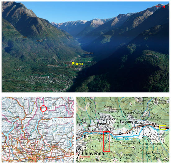
Figure 1.
Location of the study area in the Chiavenna valley, in the northern part of Italy, near the Swiss border. In the yellow and red rectangles, the case study surveyed with medium-range Terrestrial Laser Scanner (TLS) and Backpack Indoor Mobile Mapping System (IMMS) are highlighted—images taken from Google Earth Pro and map.geo.admin.ch.
The tree and shrub species forming the forest include various native entities with a prevalence of chestnut, hornbeam, ash, sycamore, linden, oak, cherry, and mountain ash.
Moreover, large and still visible landslide sediments from to the 1618 landslide, which destroyed the town and surrounding areas, are present throughout the whole region of interest [37]. The dramatic event had a very strong impact on the evolution of the valley, both in terms of geological characterization and loss of human lives; historical documentation reports the entire destruction of Piuro and Scilano villages, causing the death of 1000–2000 inhabitants. It is considered one of the most catastrophic events ever recorded in the region [38].
The research is part of the Interreg project A.M.AL.PI. 18 (Alpi in movimento, Movimento nelle ALpi. Piuro 1618), aimed at realizing a best practice to study historical behavior of dangerous hillsides applicable to all the case studies identified along the Alpine range, that extends from the Gottardo Pass to the Maloja Pass, both on Italian and Swiss territory. The ambitious goal is to increase the attractiveness of the territories of the Bregaglia-Chiavenna valley-Moesa-Ticino axis by focusing on an innovative fruition of natural and cultural resources. The project aims to demonstrate the historical specificity of the involved valleys, symbol of the richness of the Alpine routes, and to investigate the importance of geological knowledge in the prevention of natural disasters. Therefore, the research project consists of the creation of high-resolution 3D terrain models, useful to understand landslides movements of the past, integrating multi-scale and multi-techniques survey methods to produce a sort of reverse-engineering of the territory through a multidisciplinary approach involving the other A.M.AL.PI. 18 project partners. Landslides have historically occurred in the concerned territory and the hydrogeological risk is still significant today [39,40]. For this reason, high-resolution digital mapping helps improve its prevention and mitigation.
The paper presents the first part of the research that is the creation of a high-resolution DTM obtained by integrating 3D data (Point Clouds—PC) coming from several sources, starting from long and medium-range Terrestrial Laser Scanners (TLS) up to a Backpack Indoor Mobile Mapping System (IMMS). Since some specific sites are considered strategic for a proper and complete interpretation of the landslide event in the area under investigation, they are surveyed with LS techniques at a very high resolution (5 mm to 40 mm), in accordance with the other partners involved in the project.
1.3. Data Integration Framework
The integration of data characterized by different resolutions and coming from several sources is something already faced in literature. The chance of creating a multi-resolution model integrating data coming from different kinds of sensors presents the possibility to obtain a constantly updated 3D digital representation that deals with the appropriate level of detail wherever necessary. Considering the limits of a single-sensor approach and the fact that currently a sensor that works effectively in all conditions does not exist, this multi-source approach allows for creating a hybrid model that takes advantage of the potentialities of the employed instruments. Data integration is particularly investigated in the field of surveys for the documentation of complex architectures, where it allows for achieving great adaptability when taking into account 3D metric acquisition in different scenarios and where it constitutes a fundamental instrument for the analysis and interpretation of historical sites [41,42,43].
Things are different when referring to multi-source and multi-resolution surveys in the environmental field, particularly those aimed at providing DTMs for different purposes, from the modeling of gravitational phenomena, rockfall, avalanches, to surface run-off. The Heli-DEM project [44], for example, integrates data at the border territory between Italy and Switzerland in order to create a unique DTM for the alpine and subalpine area, which is useful to analyze the scenario when an event, such as a landslide, happens. Together with the aforementioned multi-source multi-resolution DTM, noteworthy data integrations were conducted at the national or even larger scale, combining data coming from preexisting DTMs with different resolutions and accuracies [45,46,47], vector contour lines from maps, break lines, geodetic points, and photogrammetric data [48].
The investigations and processing cited above include available products with a resolution from 1 m up to 100 m. Given the goal of the current project, however, it is not possible to rely only on the existing datasets, due to their inadequate resolution. The reference is to the 5 m and 20 m resolution DTMs made available by the institutions, and to the 1:10,000 contour lines. Traces left by the events that shaped the area as it appears today would not be visible, like metric and sub-metric morphological highs, erosion of riverbanks due to ancient river course, deposits of finer material, and small fractures with different dips along the sides. Consequently, the possibility of reconstructing precisely the history of the valley would be lost. The need of a big scale high-resolution DTM arises spontaneously.
Therefore, the present research wants to play a key role in the multi-resolution 3D model framework, and it is the opportunity to establish some useful workflows to speed up acquisition and processing time in different scenarios, especially those regarding the monitoring of hydrogeological instability. The resulting DTM is 0.50 m in resolution and accuracy and reaches 0.10 m resolution in specific sites identified with the other A.M.AL.PI. 18 partners, allowing for recognizing even the single rocks dropped from the slopes and deposited on the valley floor. A processed high-resolution DTM such as this one constitutes the starting point from which to assume the evolution of the landform, recognizing the thickness and disposition of the different debris deposits. This will allow for making reliable predictions about the composition of the subsoil and to produce detailed 3D geological sections in order to be able to reconstruct the territory of Piuro back in time. By progressively removing the recognizable volumes from the DTM, a series of derived DTMs corresponding to specific historical periods will be produced, up to hypothesizing how the territory was before the 1618 landslide.
2. Materials and Methods
In this study, several surveys have been conducted, using the appropriate instrument depending on the characteristics of the survey and of the instrument itself. In the following section, data acquisition and processing procedures are presented and grouped on the basis of the employed instrumentation, i.e., long-range LS, medium-range LS and IMMS. A flowchart summarizing the whole adopted methodology and a table listing pros and cons of the employed instrumentation are proposed at the end of the chapter.
2.1. Long-Range TLS RIEGL VZ-4000
Data constituting the most general DTM were collected with long-range TLS RIEGL Vz-4000 between March 2017 and October 2020. The instrument offers an extremely long range of more than 4000 m and a wide field of view of 60° vertical and 360° horizontal. These peculiarities are ideal for the acquisition of both the slopes and the valley floor of the area under investigation, since it extends for about 2.5 km both in the E-O and N-S directions. The scanner is mounted on a tripod, leveled and connected to a laptop and an external battery. The characteristics of the scans, which are the desired resolution and the area range to be surveyed, are set up in the RiSCAN PRO software (RIEGL, Horn, Austria) at the moment of the acquisition. In addition, a built-in calibrated 5-Mpixel camera capturing images deflected by the laser mirror enables the coverage of the entire field of view with an appropriate number of high-resolution images automatically stitched together to create a high-resolution panorama image. This last one enables the creation of RGB colored PCs. In addition, the possibility of recording multiple echoes becomes crucial in order to split ground/non-ground points.
A total of 7 scans (Figure 2) were acquired in the mentioned period, stationing between 450 and 900 masl—the valley floor is about 400 masl, making sure to cover the area as uniformly as possible. Despite surveying the area in times of the year when vegetation is sparser to have a better chance of getting the laser beams to the ground, scan n. 7 is characterized by dense vegetation in the area of the alluvial fan formed by the Valle Drana stream, thus not allowing an accurate ground detection. Furthermore, the high incidence angle of the laser beam did not help reach the ground in an effective way. The final total number of acquired points is 229,179,174 and the 7 scans’ principal characteristics are summarized in Table 1.
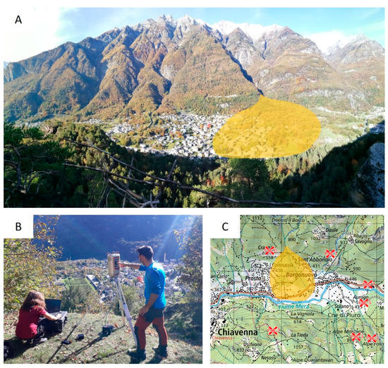
Figure 2.
(A) The valley floor and the north side of the area under study; (B) acquisition with RIEGL Vz-4000 and (C) the 7 scans position. Image modified from map.geo.admin.ch. Valle Drana stream is highlighted in orange in (A,C).

Table 1.
Characteristics of the 7 scans acquired with RIEGL Vz-4000.
Data Processing
The 7 scans were registered using 21 homologous points detected throughout the whole area, obtaining an RMS error of 0.12 m. Subsequently, they have been georeferenced using 13 points coming from an RTK GNSS survey. This procedure allowed for georeferencing the scans all at once because not all of the RTK GNSS points were visible from the 7 different positions. The RMS error related to the RTK GNSS points is 0.36 m. The obtained errors are consistent with the resolution of the PCs and the 1:2000 scale for which the final product is designed.
In order to separate ground and non-ground points, the acquired territory was divided into three homogeneous areas: the valley floor, the north side and south side (Figure 3A), due to common orographic characteristics. The surface-based Cloth Simulation Filter (CSF) algorithm [49], implemented in CloudCompare software [50], was then applied to the single + first echoes of each of the identified areas, each one tilted by ±30°, ±45° and ±60° to preserve points also in the steepest slopes. To tilt the PCs, an interpolating plane was first fitted to the involved area and then made horizontal. The specified rotation matrices were then applied to rotate the PC by the desired angle. The choice of the returns to be selected in order to extract ground points is a matter of debate [51]. The last return is considered the most reliable since it has the highest chance to reach the terrain in dense vegetated areas. However, considering the characteristics of the area under study, which is dominated by dense vegetation on both the sides but made also of large crops, fields and private gardens, even the first echo was used to extract the terrain, in addition to the last echo.
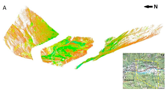
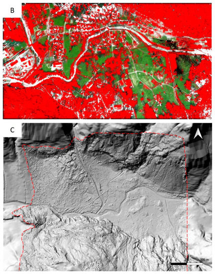
Figure 3.
(A) Division of the whole test territory into three homogeneous areas. From left to right: north side, valley floor and south side; (B) example of ground (RGB colored)—non ground (red colored) separation in a portion of the valley floor after the application of CSF algorithm; (C) comparison of the 0.50 m hillshaded DTM of the whole area, inside the red line, with the 5 m regional hillshaded DTM.
The CSF algorithm plugin is simple to use thanks to the limited number of integer and Boolean parameters to be set. It is based on the cloth simulation 3D computer graphics algorithm [52] and consists of inverting the PC and applying a rigid cloth to it. By analyzing the interactions between the cloth nodes and the corresponding points of the PC, it is possible to define the final shape of the cloth. The plug-in allows for setting the type of terrain, which can be a steep slope, relief, or flat, which then determines the rigidness of the cloth. When dealing with very steep slopes, the internal constraints among particles do not allow a proper reconstruction of the ground. For this reason, there is the possibility to select an extra option to solve the problem. The second step involves the setting of cloth parameters. The resolution refers to the grid size of the cloth used to cover the terrain. The higher the resolution, the sparser the selection of ground points. The classification threshold defines the maximum distance inside which the points of the PC are then taken into consideration to be eventually added to the ground points set. Finally, it is possible to set the maximum number of iterations of the process.
The CSF algorithm was then applied to the 21 obtained PCs—the horizontal ones were also used to extract ground points. After several tests, the final ground points were obtained selecting a 0.50 m cloth resolution and a 0.10 m classification threshold. The obtained points (more than 42 millions) were interpolated in ArcGIS Pro (Esri, Redlands, California) [53], setting a 0.50 m raster cell and using the Inverse Distance Weighting (IDW) algorithm (Figure 3C), which is considered to be a good interpolation technique thanks to a reasonable computational time and the non-addition of artefacts in the final product [29]. Considering the location of the area, the WGS84 UTM 32N projection was assigned to the output raster.
2.2. Medium-Range TLS Leica RTC360
TLS Leica RTC360 is used to collect data in the “Belfort” archaeological site (Figure 4), an area considered strategic for a proper and complete interpretation of the 1618 landslide. Located in the eastern side of the region of interest (highlighted in yellow in Figure 1), the site extends for about 1 ha and is one of the rare remaining and escaped examples of the antique Piuro village before being destroyed by the 1618 landslide. The geometry is very challenging, considering the presence of subways, caves, very high vertical stone walls, and dense vegetation all around.
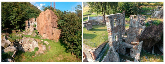
Figure 4.
The “Belfort” archaeological site, characterized by dense vegetation and complex geometry.
Two surveys were performed between September and November 2019, reconstructing the area by means of 122 scans. The first 104 were collected during the first survey, while the last 18, which were necessary to complete the far eastern section, were collected during the second one.
Thanks to the scanner’s 360° horizontal and 300° vertical field of view, even the most closed and narrow environments have been completely acquired without any problems. The acquisition is very fast because the scanner is self-leveling and every scan only requires less than 3 minutes, setting the highest resolution of 3 mm at 10 m. The simultaneous acquisition of full spherical HDR images through the incorporated 36 Mpixel camera allows for obtaining the RGB information to color the PC. Moreover, the PCs are automatically pre-aligned directly on field without using any targets thanks to the real-time tracking of scanner movement between setups based on Visual Inertial System (VIS) [54].
At the end of the survey, the final total number of acquired points was 8,444,710,903.
Data Processing
As mentioned above, the 122 scans were automatically pre-aligned in the associated software Leica Cyclone REGISTER360 (Leica, Wetzlar, Germany) [54]. After an extensive manual cleaning operation and a coarse vegetation removal to improve the final alignment, links among scans were refined and added, obtaining a 4 mm alignment error. Considering that the survey was also conducted in two different months, September and November, the dense vegetation present in the area showed differing characteristics, adversely affecting the alignment phase. For this reason, it was removed from the project. All of the scans were then subsampled to 1 cm with a regular density reduction and subsequently merged, in order to obtain an easier to manage a unique product of 275,968,682 points. The PC was then georeferenced by means of 6 RTK GNSS points, with an RMS error of 0.036 m. Due to the change in scale, when compared to the long-range acquisition, two different approaches had been considered to separate points belonging to the ground. The first was the same CSF algorithm used with the long-range PCs, and the second was a Machine Learning (ML) approach based on the methodology developed in [55,56].
The ML approach uses a Random Forest (RF) classifier trained and evaluated on a manually annotated portion of the dataset (17% of the total number of points) composed of a total of nine semantic classes, together with computed geometric covariance features. The complexity of the area (presence of ancient ruins, caves, dense vegetation) proved a real challenge to the attribution of semantic meaning to the PC. The small amount of required labeled data and the speed of the training process make the RF classifier a good choice; nonetheless, the complex morphology of the surveyed area introduced a higher uncertainty during the selection of the correct training dataset. The 9 considered classes are: building, ground, bridge, fence, tie rods, electric wire, street retaining wall, trellis, and vegetation (Figure 5).
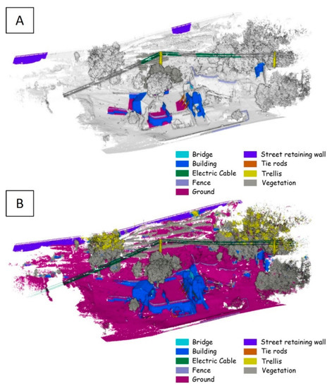
Figure 5.
(A) Training set (10% of the total PC) and (B) obtained classification of the Belfort archaeological site with the ML RF algorithm. 94.56% overall acc.; 79.35% avg. recall; 82.43% avg. F1 score.
Classification results proved satisfactory (94.56% overall acc.; 79.35% avg. recall; 82.43% avg. F1 score) and comparable to the application of the CSF algorithm. However, the time required to find the correct training set, manually segment it, compute geometric features for the whole PC, and spread the classification to the entire area made the CSF a better alternative for its faster application. This is because only the distinction among ground and non-ground points counts for the DTM generation. The ML RF approach would better suit an architectonic dataset that needs a finer classification. For these kinds of datasets, the geometric features distribution among the same class is more uniform and allows the algorithm to better distinguish among different elements. For instance, columns have a certain curvature, and it is remarkably different from that of a floor, thus allowing the algorithm to clearly distinguish among them. For the case study at hand, the covariance features that describe bare ground points are easily confused with those describing rocks and caves, introducing a strong degree of confusion.
The CSF algorithm was tested on a 5 cm subsampled PC (16,160,360 points). The complexity of the archaeological site demanded a large number of tests before finding the optimal parameters and a significant part of manual labor to select all the correct ground points. Considering the operation of the algorithm, to improve the result, those environments like caves and similar were removed before applying it. The resulting points, 4,272,027, were obtained, setting both the cloth resolution and the classification threshold equal to 0.10 m. Subsequently, they were interpolated in ArcGIS Pro, setting a 0.10 m raster cell and using the IDW algorithm again for the reasons explained above (Figure 6B). The WGS84 UTM 32N projection was assigned to the output raster.
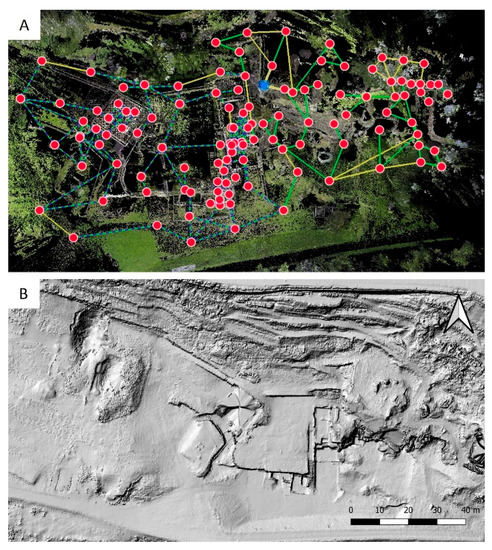
Figure 6.
(A) Position scheme of the 122 scans to survey the “Belfort” archaeological site and links among them; (B) the obtained 0.10 m DTM appropriately hillshaded.
2.3. Backpack LS IMMS Heron MS Twin
Moving towards the hillside, in the areas where dense vegetation prevails and the high incidence of long-range TLS rays and the morphological characteristics of the slope do not allow a proper terrain reconstruction, a Backpack IMMS campaign is done both (i) to obtain higher resolution data of a territory otherwise inaccessible and hidden using other survey techniques, and (ii) to simultaneously test the geometric accuracy that is achievable by an instrument relying on SLAM (Simultaneous Localization And Mapping) technology and strongly tested in such a challenging scenario, with continuous changes of slopes and constant presence of vegetation—trees and evergreen shrubs [57,58].
The surveyed territory is part of a natural reserve. Here, the glacial morphology, characterized by steep slopes, deep cracks, and cliffs, is particularly evident. Ancient caves called “Trone” present along the path are also surveyed. All these factors constitute an excellent test bench for an IMMS survey that is strongly tested since the typical recommendations implemented when dealing with SLAM algorithms are missing. Commonly, in order to refine the point cloud registration along the trajectory, it is recommended to set up a survey scheme made up of closed loops in order to create some rigid constraints that allow for adjusting both horizontal and vertical errors, following a principle similar to the one of the closed polygonal. This means starting and ending the survey at the same point and passing through the same portion of the surveyed environment at different times. The path is about 3 km long with an altitude difference of approximately 350 m, starting from 700 masl and ending at 360 masl (highlighted in red in Figure 1). It took two different days, one in October 2020 and the other one in March 2021, because of storage issues faced during the first day. The Backpack IMMS Heron MS Twin, produced by Gexcel [59], was used to perform the survey (Figure 7). The instrument is characterized by two LiDAR Velodyne Puck sensors, one rotating on the vertical axis and the other one on a 45° tilted axis, which provide 360° horizontal FOV (Field Of View) and 30° vertical FOV each. While walking, it is possible to check in real time the surveyed environment thanks to a portable tablet that can be carried with a dedicated harness, leaving the hands free. The automatic acquisition at 15 Hz of spherical images (1920 × 1080 pixel) makes it possible to color the PC. A total of 7 trajectories were acquired, stopping the acquisition when the operator needed to rest and took about two hours to complete the survey. Their main characteristics are summed up in Table 2. As said before, the slope conformation did not allow for creating well-structured rigid constraints along the trajectory. However, closed loops were built where feasible, precisely in the central part of the trajectory, going off the path without putting the operator in trouble.
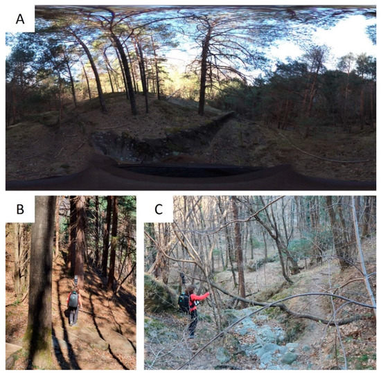
Figure 7.
(A) Example of a spherical image acquired by Heron MS Twin; (B,C) represent moments of the survey.
Table 2.
Heron MS Twin trajectories main characteristics.
Some portions of the surveyed path, reported as an example in Figure 7C, were also quite challenging to survey: the presence of dense stuck branches risked damaging the instrument, with the consequent risk of losing the calibration of the cameras on the top of the pole. In such cases, a second person present in the field helped prevent dangerous situations, alerting the operator when needed.
While walking to reach the upper part of the hillside from which to start the survey, a total of 5 RTK GNSS points were taken in those areas where the cover provided by the vegetation made it possible. Although limited, they are essential for a proper trajectory reconstruction.
Data Processing
The 7 trajectories were reconstructed and processed with Heron Desktop software (Gexcel, Brescia, Italy) [59], following the implemented four-step workflow. The numerous parameters that were set throughout the procedure gave the possibility to operate at will, according to the sensitivity of the operator. Once estimated, the trajectory by checking the accordance between the IMU (Inertial Measurement Unit) and the alignment of the scans (Figure 8A), the third part of the workflow involves the drift effect reduction by creating links all along the trajectory. In this step, it is possible to insert static scans in order to better constrain the IMMS PC. For this purpose, four scans were acquired with TLS FARO Focus 3D × 330 in correspondence with the final part of the surveyed path, paying attention to detect the most possible three-dimensional geometries in order to produce even more rigid constraints. Before being imported into Heron Desktop, they were georeferenced by means of 12 RTK GNSS points, achieving a mean registration error of 0.028 m.
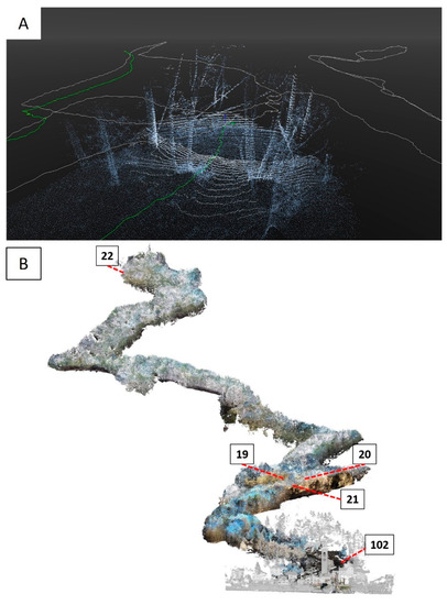
Figure 8.
(A) Trajectory reconstruction with Heron Desktop; (B) the total obtained PC once exported in Reconstructor® and aligned to the FARO Focus 3D × 330 scans. Labels refer to the RTK GNSS points used to adjust the trajectory.
In this phase of the process, it was possible to select specific points in the PC and assign known coordinates and the relative accuracy, named “Heron accuracy” in Table 3. The 5 RKT GNSS points were then added as constraints in order to adjust the trajectory. Specifications of the used points are summarized in Table 3.
Table 3.
RTK GNSS points used to adjust the Heron MS Twin trajectory. The mentioned optimization refers to the iterative process that concludes the trajectory reconstruction phase, in which the creation of rigid links among the IMMS PC and, if available, static scans, and the use of points with known coordinates allow a proper reconstruction.
At the end of an optimization iterative process, in which every link created to strengthen the trajectory is checked and, if needed, refined, the trajectories are exported to Reconstructor® software (Gexcel, Brescia, Italy) [59]. During this phase, it is possible to remove ghost points. This is very useful in case, for example, there are people walking near the surveyor. It is also possible to select a proper range around the sensor in order to export only the useful points. In the present case, a 1–30 m range was selected. Finally, a 0.05 m voxelization was chosen to speed up processing. The exported PC is reported in Figure 8B.
In order to separate ground/non-ground points, in this case, the CSF algorithm was also adopted. Due to the almost constant slope of the surveyed path, the PC was processed all at once. A cloth resolution of 0.20 m and a classification threshold of 0.50 m has ensured the preservation of rocks above the ground level, required for a correct representation of the territory. However, such a threshold has resulted in an incomplete trees removal: the part of the trunk closest to the ground was preserved. For this reason, the CSF algorithm was implemented again on the ground points that were just extracted. This time, a cloth resolution of 0.10 m and a classification threshold of 0.10 m were adopted, allowing for obtaining a correct result.
The obtained 15,707,444 points were interpolated in ArcGIS Pro setting a 0.10 m raster cell and using again the IDW algorithm to compute the DTM. The WGS84 UTM 32N projection was assigned to the output raster, reported in Figure 9.
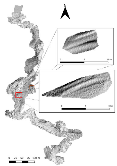
Figure 9.
The 0.10 m hillshaded DTM obtained by interpolating ground points coming from the Heron MS Twin survey. Details of rocks affected by the shaping action of the huge ice flow descending along the entire Chiavenna valley during the last glaciation are reported with a higher scale.
2.4. Unique Multi-Resolution DTM
The last step necessary to obtain a unique multi-resolution DTM is to integrate the different terrain models processed so far. To do this, a mosaic is created using the homonymous function available in ArcGIS Pro. The function returns a unique grid whose resolution coincides with the minimum DTM cell; in this case, it was 0.10 m. The projected reference system WGS84 UTM 32N is associated with the output raster.
A table listing pros and cons of the employed instrumentation is reported in Table 4, while a flowchart summarizing the whole adopted methodology is provided in Figure 10.
Table 4.
Overview of pros and cons of the employed instrumentation.
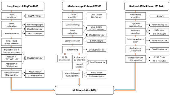
Figure 10.
Flowchart summarizing the entire adopted methodology to obtain the multi-resolution DTM.
3. Results
A quality assessment is reported for each one of the three generated DTMs. Vertical and horizontal accuracies are reported in Table 5. They are calculated by means of standard deviation of residuals, as reported in Equation (1):
where SD refers to Standard Deviation, α corresponds to X, Y, Z coordinates and
Δαi = αi,DTM − αi,CHECK
Table 5.
Vertical and horizontal SD of residuals for each of the generated DTMs. Unit of measures: meter.
The extensive RTK GNSS campaign, resulting in the acquisition of almost 200 points over the entire valley floor of the test area, allowed for computing the SD on a representative sample of check points. ΔZ of the three DTMs is reported in Figure 11.
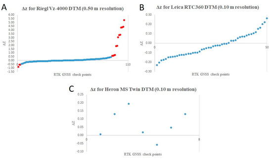
Figure 11.
Difference in Z coordinate between RTK GNSS check points and DTM coming from TLS RIEGL Vz-4000 (A), TLS Leica RTC360 (B), and Backpack IMMS Heron MS Twin (C).
In Figure 11A, check points for which Δz exceeds the threshold value for a 1:2000 scale representation are colored in red. Threshold value is set in a conservative way at 0.50 m. Those points correspond to RTK GNSS points surveyed in the Belfort archaeological area, which has not been properly reconstructed in the 0.50 m resolution DTM. Considering that the final unique multi-resolution DTM has the accuracy attributable to the Leica RTC360 DTM in the Belfort archaeological site, if red points are removed from the SD calculation, it decreases to 0.176 m, respecting the scale representation error.
Another important vertical accuracy check for the 0.50 m resolution DTM is carried out on the south side, in the red-highlighted area in Figure 1. Here, RTK GNSS points were collected to improve the Backpack IMMS PC accuracy. SD is calculated on the three points acquired while walking and is equal to 6.525 m. This kind of result is not unexpected. In this regard, some consideration must be made. Vegetation is very dense in that area and the incidence of LS is high due to the scan position. Even if RIEGL Vz-4000 registers multiple echoes, the probability of reaching the ground is almost null. Moreover, the distance from the scan position causes a low points density. For this reason, the interpolated DTM resulted in an incorrect ground reconstruction, degrading the vertical accuracy when moving towards the side.
Regarding the DTM produced with Backpack IMMS Heron MS Twin, by looking at the plot reported in Figure 11C, the accuracy seems adequate for the obtained product. However, it provides partial information since there are also those used for the improvement of the accuracy in the Heron Desktop software optimization phase among the points used for the calculation of the SD. A global vertical accuracy check is therefore conducted by subtracting the 5 m resolution DTM, made available by the institutions, to the 0.10 m resolution deriving from the Backpack IMMS. The decision to use the 5 m DTM instead of the 0.50 m one comes from the observation previously made about the incorrect reconstruction of the ground in this densely vegetated area. The histogram of the DTMs differences is shown in Figure 12.
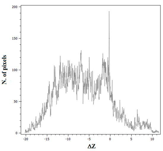
Figure 12.
Difference in Z coordinate between 5 m resolution DTM made available by the institutions and 0.10 m resolution DTM obtained with Heron MS Twin.
Numerous considerations can be made, both about the processing and the obtained results. As for the use of CSF algorithm to separate ground/non-ground points, no manual operation was required to better perform the algorithm when applied to the long-range TLS RIEGL Vz-4000 PC, considering that data were acquired from higher station points with respect to the height of the ground. However, when dealing with the PCs coming from the medium-range TLS Leica RTC360 and Backpack IMMS Heron MS Twin, caves and rooms situated underground were previously manually segmented, losing some of the benefit of using an automated points extraction algorithm. In fact, the presence of underground areas makes it difficult to correctly select points belonging to the terrain since the algorithm turns the PC upside down.
As for the survey conducted with Backpack IMMS Heron MS Twin, tests conducted to reconstruct the trajectory in a proper way have demonstrated the need for points with known coordinates, acquired with a regular frequency, to be added during the optimization phase. In the case reported, the maximum drift error is obtained at a distance of about 350 m from RTK GNSS points 19, 20, and 21, and it consists of about 20 m in the Z-direction. The result is explained when checking the accuracy of the obtained DTM, in Figure 12, and is something expected considering the challenging conditions under which the survey was carried out. As stated in 2.3., the SLAM algorithms need specific practices in order to perform well, and they were not guaranteed.
Regarding the high-resolution DTMs, the 0.50 m DTM obtained by processing RIEGL Vz-4000 PC clearly shows its value. Figure 13 compares the same areas (A–B and C–D) visible in the 0.50 m DTM (A and C) and in the 5 m DTM (B and D) made available by the Institutions. By comparison, it is evident how the high-resolution DTM allows for detecting precisely the incision rate that the Mera river achieves on the sediments (Figure 13C), giving the opportunity to conduct a quantitative analysis. Figure 13A then shows old river-bed traces that are essential to study the evolution of the valley. Such details are invisible on the 5 m DTM and make the high-resolution DTM crucial for the purpose of the A.M.AL.PI. 18 project.
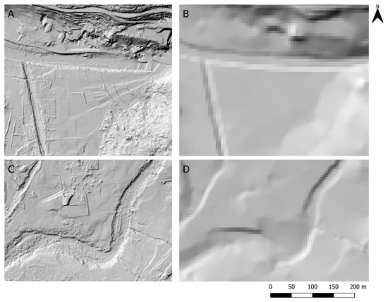
Figure 13.
Comparison of the details detectable on the DTMs with different resolutions. Mera river’s old bed traces are visible on the 0.50 m hillshaded DTM (A), while they cannot be distinguished on the Regional 5 m hillshaded DTM (B). Incision rate achieved on the sediments by Mera river is clearly visible in the 0.50 m DTM (C) whereas it is barely visible on the 5 m DTM (D).
The 0.10 m DTM obtained by processing Leica RTC360 PC related to the Belfort archaeological site is reported in Figure 14 and compared to the same area visible on the 0.50 m DTM. In this case as well, the added value clearly comes to light. It is sufficient to observe that, in the low resolution DTM (on the right), entire portions of the terrain are missing, thus mystifying the reconstruction of the area and creating negative volumes of rock masses (dark areas in the central part of the right image).
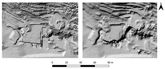
Figure 14.
Comparison of Belfort archaeological site hillshaded DTMs obtained starting from the Leica RTC360 ground points (on the left) and from RIEGL Vz-4000 ground points (on the right).
Regarding the high-resolution 0.10 m DTM processed starting from the Backpack IMMS Heron MS Twin, in Figure 9, two details are enhanced. They refer to outcropping rocks where the shaping action of the ice flow occupying the Chiavenna valley is particularly evident. Details, such as these highlighted, are very precious because they are not visible in any other type of survey, given their location. Moreover, considering that one of the main objectives of the A.M.AL.PI. 18 project is the innovative use of natural resources, a digital reconstruction of an area comprised in a natural reserve could become crucial to establish novel attractiveness strategies.
Along with these virtuous examples, however, it is also necessary to identify areas that have not been properly reconstructed. As mentioned in Section 2.1, one of the scans conducted with long-range TLS was characterized by very dense vegetation in the area of the alluvial fan formed by the Valle Drana stream. Together with the high incidence angle of the laser beam, it has resulted in an incorrect ground reconstruction, detectable in the 0.50 m DTM, as reported in Figure 15. The points classified with the CSF algorithm have a low density and, given the circumstances of the survey, could easily belong to the crowns of the trees.
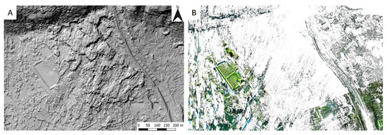
Figure 15.
(A) The alluvial fan formed by the Valle Drana stream improperly reconstructed in the 0.50 m DTM; (B) points classified as ground extracted with the CSF algorithm.
4. Discussion and Conclusions
The paper presents the first part of an ambitious project aimed at realizing a best practice to study historical behavior of dangerous hillsides. Considering the goal of the A.M.AL.PI. 18 project, the presented research includes the creation of high-resolution multi-source 3D terrain models obtained by integrating 3D data coming from different types of Laser Scanning instruments.
Numerous challenges were faced, both due to the characteristics of the test area and to the processed Point Clouds (PCs). Regarding data coming from the long-range Terrestrial Laser Scanner (TLS), the valley conformation has caused the application of the ground points filtering procedure three times in order to also preserve points in the steepest regions. This resulted in tripling the processing time, which was already onerous, given the amount of data to be analyzed. In addition, the dense vegetation present during the second survey and the incidence of the laser scanner rays in a portion of the valley floor gave rise to artifacts that are hard to remove, as illustrated in Figure 15.
Processing and managing the scans acquired with the medium-range TLS was not easy. A huge calculation capacity was required, due to their number and size. Moreover, the presence of caves and other underground spaces demanded a significant manual labor when running the Cloth Simulation Filter (CSF) algorithm to obtain all the correct ground points. The additional test involving the Machine Learning (ML) Random Forest (RF) classification to extract ground points did not bring noticeable advantages, due to the environmental scale of the archaeological site with presence of vegetation. This increases the degree of confusion of the geometric covariance features among the different classes.
The Backpack Indoor Mobile Mapping System (IMMS) survey was a very interesting test to verify how to improve the accuracy of the system, considering that the typical recommendations to be implemented when dealing with Simultaneous Localization And Mapping (SLAM) algorithm were missing. In addition, since the path was entirely reconstructed thanks to two surveys performed during different periods of the year, the matching algorithm to strengthen the trajectory was incredibly stressed. This was due to the presence–absence of leaves on the trees, resulting in an accuracy degradation.
The added value that the final multi-resolution Digital Terrain Model (DTM) brings to the research is clear and broadly demonstrated. Future works aimed at improving the result could regard an ad hoc survey of the alluvial fan formed by the Valle Drana stream. Considering the accessibility of the area thanks to numerous pathways, a Backpack IMMS survey could be the best choice.
Regarding the accuracy check, since the RTK GNSS campaign that has been conducted up until now mainly focuses the valley floor, it would be useful and proper to include both sides in a forthcoming survey.
Lastly, a photogrammetric approach could be added to the SLAM algorithms at the base of the Backpack IMMS to improve the achievable accuracy in those environments where the typical SLAM recommendations are hard to implement. Visual SLAM performs well. By combining the two technologies, promising results could be obtained.
Author Contributions
Conceptualization, F.F.; methodology, F.M. and S.T.; validation, F.M. and G.P.M.V.; investigation, F.M. and S.T.; resources, G.P.M.V. and F.F.; writing—original draft preparation, F.M.; writing—review and editing, F.M., S.T., C.A., G.P.M.V. and F.F.; supervision, C.A. and F.F.; project administration, C.A.; funding acquisition, C.A. All authors have read and agreed to the published version of the manuscript.
Funding
The present work was co-funded through the Interreg V-A Italy-Switzerland Cooperation Program—A.M.AL.PI.2018 “Alpi in Movimento, Movimento nelle Alpi. Piuro 1618-2018”, ID 594274–Axis 2 “Cultural and natural enhancement” of the Cooperation Program IT-CH 2014-2020.
Data Availability Statement
The data presented in this study are available on request from the corresponding author. The data are not publicly available since the Interreg V-A Italy-Switzerland Cooperation Program—A.M.AL.PI.2018 is still in progress.
Acknowledgments
The authors would like to thank Scuola Universitaria Professionale della Svizzera Italiana (SUPSI), in particular Eng. Alessio Spataro for the long-range surveys. Significant thanks go to Gexcel S.r.l., in particular to Ph.D. Eng. Matteo Sgrenzaroli for his precious support in data processing. Finally, the authors would also thank Enrico Pigazzi for the valuable support in the geological interpretation of the obtained results.
Conflicts of Interest
The authors declare no conflict of interest.
References
- Joyce, K.E.; Samsonov, S.V.; Levick, S.R.; Engelbrecht, J.; Belliss, S. Mapping and monitoring geological hazards using optical, LiDAR, and synthetic aperture RADAR image data. Nat. Hazards 2014, 73, 137–163. [Google Scholar] [CrossRef]
- Tarolli, P.; Arrowsmith, J.R.; Vivoni, E.R. Understanding earth surface processes from remotely sensed digital terrain models. Geomorphology 2009, 113, 1–3. [Google Scholar] [CrossRef]
- Tarolli, P. High-resolution topography for understanding Earth surface processes: Opportunities and challenges. Geomorphology 2014, 216, 295–312. [Google Scholar] [CrossRef]
- Toschi, I.; Allocca, M.; Remondino, F. Geomatics Mapping of natural hazards: Overview and experiences. Int. Arch. Photogramm. Remote Sens. Spat. Inf. Sci. ISPRS Arch. 2018, 42, 505–512. [Google Scholar] [CrossRef]
- Toschi, I.; Remondino, F.; Kellenberger, T.; Streilein, A. A survey of geomatics solutions for the rapid mapping of natural hazards. Photogramm. Eng. Remote Sens. 2017, 83, 843–859. [Google Scholar] [CrossRef]
- Giordan, D.; Hayakawa, Y.S.; Nex, F.; Remondino, F.; Tarolli, P. Review article: The use of remotely piloted aircraft systems (RPAS) for natural hazards monitoring and management. Nat. Hazards Earth Syst. Sci. 2018, 18, 3085–3087. [Google Scholar] [CrossRef]
- Casagli, N.; Frodella, W.; Morelli, S.; Tofani, V.; Ciampalini, A.; Intrieri, E.; Raspini, F.; Rossi, G.; Tanteri, L.; Lu, P. Spaceborne, UAV and ground-based remote sensing techniques for landslide mapping, monitoring and early warning. Geoenviron. Disasters 2017, 4, 1–23. [Google Scholar] [CrossRef]
- Guha-Sapir, D.; Hargitt, D.; Hoyois, P. Thirty Years of Natural Disasters 1974–2003: The Numbers; PUL: Lovain-la-Neuve, Belgium, 2004; ISBN 2930344717. [Google Scholar]
- Scaioni, M.; Longoni, L.; Melillo, V.; Papini, M. Remote sensing for landslide investigations: An overview of recent achievements and perspectives. Remote Sens. 2014, 6, 9600–9652. [Google Scholar] [CrossRef]
- Chang, K.J.; Chan, Y.C.; Chen, R.F.; Hsieh, Y.C. Geomorphological evolution of landslides near an active normal fault in northern Taiwan, as revealed by lidar and unmanned aircraft system data. Nat. Hazards Earth Syst. Sci. 2018, 18, 709–727. [Google Scholar] [CrossRef]
- Dewitte, O.; Jasselette, J.-C.; Cornet, Y.; Van Den Eeckhaut, M.; Collignon, A.; Poesen, J.; Demoulin, A. Tracking landslide displacements by multi-temporal DTMs: A combined aerial stereophotogrammetric and LIDAR approach in western Belgium. Eng. Geol. 2008, 99, 11–22. [Google Scholar] [CrossRef]
- Roemer, H.; Kaiser, G.; Sterr, H.; Ludwig, R. Using remote sensing to assess tsunami-induced impacts on coastal forest ecosystems at the Andaman Sea coast of Thailand. Nat. Hazards Earth Syst. Sci. 2010, 10, 729–745. [Google Scholar] [CrossRef]
- Witek, M.; Jeziorska, J.; Niedzielski, T. An experimantal approach to verifying prognoses of floods using unmanned aerial vehicle. Meteorol. Hydrol. Water Manag. 2014, 2, 3–12. [Google Scholar] [CrossRef]
- Deffontaines, B.; Chang, K.-J.; Champenois, J.; Lin, K.-C.; Lee, C.-T.; Chen, R.-F.; Hu, J.-C.; Magalhaes, S. Active tectonics of the onshore Hengchun fault using UAS DSM combine with ALOS PS-InSAR time series (Southern Taiwan). Nat. Hazards Earth Syst. Sci. 2018, 18, 829–845. [Google Scholar] [CrossRef]
- Cunningham, D.; Grebby, S.; Tansey, K.; Gosar, A.; Kastelic, V. Application of airborne LiDAR to mapping seismogenic faults in forested mountainous terrain, southeastern Alps, Slovenia. Geophys. Res. Lett. 2006, 33, 3–7. [Google Scholar] [CrossRef]
- Kondo, H.; Toda, S.; Okumura, K.; Takada, K.; Chiba, T. A fault scarp in an urban area identified by LiDAR survey: A Case study on the Itoigawa-Shizuoka Tectonic Line, central Japan. Geomorphology 2008, 101, 731–739. [Google Scholar] [CrossRef]
- Li, Z.; Miao, Y.; Fa, G.; Wang, Z.; Shao, X. Use Remote Sensing to Detect the Geomorphologic Change and its Effect around Barrow, Us Area. In IOP Conference Series: Earth and Environmental Science; IOP Publishing: Tokyo, Japan, 2020; Volume 581, p. 012046. [Google Scholar] [CrossRef]
- Lin, X.; Fangi, D.S.; Li, F.F. Acqusition of high-precision digital terrain model using P-band airborne repeat-pass SAR interferometry. In Proceedings of the 2016 CIE International Conference on Radar (RADAR), Guangzhou, China, 10–13 October 2016; pp. 1–4. [Google Scholar] [CrossRef]
- Lee, S.K.; Fatoyinbo, T.; Lagomasino, D.; Osmanoglu, B.; Feliciano, E. Ground-level digital terrain model (DTM) construction from TanDEM-X InSAR data and WorldView stereo-photogrammetric images. In Proceedings of the 2016 IEEE International Geoscience and Remote Sensing Symposium (IGARSS), Beijing, China, 10–15 July 2016; pp. 6040–6042. [Google Scholar] [CrossRef]
- Chen, Z.; Gao, B.; Devereux, B. State-of-the-Art: DTM Generation Using Airborne LIDAR Data. Sensors 2017, 17, 150. [Google Scholar] [CrossRef]
- Chen, R.F.; Chang, K.J.; Angelier, J.; Chan, Y.C.; Deffontaines, B.; Lee, C.T.; Lin, M.L. Topographical changes revealed by high-resolution airborne LiDAR data: The 1999 Tsaoling landslide induced by the Chi-Chi earthquake. Eng. Geol. 2006, 88, 160–172. [Google Scholar] [CrossRef]
- Hung, C.-L.J.L.J.; Tseng, C.-W.C.-M.M.W.; Huang, M.-J.J.; Tseng, C.-W.C.-M.M.W.; Chang, K.-J.J. Multi-temporal high-resolution landslide monitoring based on uas photogrammetry and uas lidar geoinformation. In Proceedings of the International Archives of the Photogrammetry, Remote Sensing and Spatial Information Sciences—ISPRS Archives, Prague, Czech Republic, 3–6 September 2019; Volume 42, pp. 157–160. [Google Scholar]
- Hsieh, Y.C.; Chan, Y.C.; Hu, J.C. Digital elevation model differencing and error estimation from multiple sources: A case study from the Meiyuan Shan landslide in Taiwan. Remote Sens. 2016, 8, 199. [Google Scholar] [CrossRef]
- Rocha, J.; Duarte, A.; Silva, M.; Fabres, S.; Vasques, J.; Revilla-Romero, B.; Quintela, A. The importance of high resolution digital elevation models for improved hydrological simulations of a mediterranean forested catchment. Remote Sens. 2020, 12, 3287. [Google Scholar] [CrossRef]
- Jones, A.F.; Brewer, P.A.; Johnstone, E.; Macklin, M.G. High-resolution interpretative geomorphological mapping of river valley environments using airborne LiDAR data. Earth Surf. Process. Landforms 2007, 32, 1574–1592. [Google Scholar] [CrossRef]
- Loibl, D.; Lehmkuhl, F. High-resolution geomorphological map of a low mountain range near Aachen, Germany. J. Maps 2013, 9, 245–253. [Google Scholar] [CrossRef]
- Szypuła, B. Digital elevation models in geomorphology. In Hydro-Geomorphology: Models and Trends; Shukla, D.P., Ed.; IntechOpen: London, UK, 2017; pp. 81–112. [Google Scholar]
- Jaboyedoff, M.; Oppikofer, T.; Abellán, A.; Derron, M.H.; Loye, A.; Metzger, R.; Pedrazzini, A. Use of LIDAR in landslide investigations: A review. Nat. Hazards 2012, 61, 5–28. [Google Scholar] [CrossRef]
- Razak, K.A.; Santangelo, M.; Van Westen, C.J.; Straatsma, M.W.; de Jong, S.M. Generating an optimal DTM from airborne laser scanning data for landslide mapping in a tropical forest environment. Geomorphology 2013, 190, 112–125. [Google Scholar] [CrossRef]
- Ghuffar, S.; Székely, B.; Roncat, A.; Pfeifer, N. Landslide displacement monitoring using 3D range flow on airborne and terrestrial LiDAR data. Remote Sens. 2013, 5, 2720–2745. [Google Scholar] [CrossRef]
- Hsieh, Y.C.; Chan, Y.C.; Hu, J.C.; Chen, Y.Z.; Chen, R.F.; Chen, M.M. Direct measurements of bedrock incision rates on the surface of a large dip-slope landslide by multi-period airborne laser scanning DEMs. Remote Sens. 2016, 8, 900. [Google Scholar] [CrossRef]
- Schmaltz, E.; Steger, S.; Bell, R.; Glade, T.; van Beek, R.; Bogaard, T.; Wang, D.; Hollaus, M.; Pfeifer, N. Evaluation of Shallow Landslides in the Northern Walgau (Austria) Using Morphometric Analysis Techniques. Procedia Earth Planet. Sci. 2016, 16, 177–184. [Google Scholar] [CrossRef][Green Version]
- Deffontaines, B.; Chang, K.-J.; Lee, C.-T.; Magalhaes, S.; Serries, G. Neotectonics of the Southern Hengchun Peninsula (Taiwan): Inputs from high resolution UAS Digital Terrain Model, updated geological mapping and PSInSAR techniques. Tectonophysics 2019, 767, 128149. [Google Scholar] [CrossRef]
- Pirotti, F.; Tarolli, P. Suitability of LiDAR point density and derived landform curvature maps for channel network extraction. Hydrol. Process. 2010, 24, 1187–1197. [Google Scholar] [CrossRef]
- Glenn, N.F.; Streutker, D.R.; Chadwick, D.J.; Thackray, G.D.; Dorsch, S.J. Analysis of LiDAR-derived topographic information for characterizing and differentiating landslide morphology and activity. Geomorphology 2006, 73, 131–148. [Google Scholar] [CrossRef]
- Soldati, M.; Borgatti, L.; Cavallin, A.; De Amicis, M.; Frigerio, S.; Giardino, M.; Mortara, G.; Pellegrini, G.B.; Ravazzi, C.; Surian, N.; et al. Geomorphological evolution of slopes and climate changes in Northern Italy during the late quaternary: Spatial and temporal distribution of landslides and landscape sensitivity implications. Geogr. Fis. Din. Quat. 2006, 29, 164–183. [Google Scholar]
- Scaramellini, G. La frana di Piuro del 4 settembre 1618, un disastro naturale di risonanza europea. Quad. Geodin. Alp. Quat. 2011, 10, 239–242. [Google Scholar]
- Pigazzi, E.; Apuani, T.; Bersezio, R.; Camera, C.; Comunian, A.; Lualdi, M.; Morcioni, A. A multidisciplinary approach to improve and share the understanding of landslide hazard in mountain environments: The PIURO 1618 disaster. In Proceedings of the EGU General Assembly Conference Abstracts, online, 19–30 April 2021. EGU2021-14567. [Google Scholar] [CrossRef]
- Paranunzio, R.; Chiarle, M.; Laio, F.; Nigrelli, G.; Turconi, L.; Luino, F. New insights in the relation between climate and slope failures at high-elevation sites. Theor. Appl. Climatol. 2019, 137, 1765–1784. [Google Scholar] [CrossRef]
- Trigila, A.; Iadanza, C.; Bussettini, M.; Lastoria, B. Dissesto idrogeologico in Italia: Pericolosità e indicatori di rischio—Edizione 2018. Ispra Rapp. 2018, 287, 2018. [Google Scholar]
- Patrucco, G.; Rinaudo, F.; Spreafico, A. Multi-source approaches for complex architecture documentation: The “palazzo ducale” in gubbio (perugia, Italy). ISPRS Ann. Photogramm. Remote Sens. Spat. Inf. Sci. 2019, 42, 953–960. [Google Scholar] [CrossRef]
- Monego, M.; Previato, C.; Bernardi, L.; Menin, A.; Achilli, V. Investigating Pompeii: Application of 3D geomatic techniques for the study of the Sarno Baths. J. Archaeol. Sci. Rep. 2019, 24, 445–462. [Google Scholar] [CrossRef]
- Chiabrando, F.; Sammartano, G.; Spanò, A.; Spreafico, A. Hybrid 3D models: When geomatics innovations meet extensive built heritage complexes. ISPRS Int. J. Geo Inf. 2019, 8, 124. [Google Scholar] [CrossRef]
- Biagi, L.; Carcano, L.; Lucchese, A.; Negretti, M. Creation of a multiresolution and multiaccuracy DTM: Problems and solutions for HELI-DEM case study. Int. Arch. Photogramm. Remote Sens. Spat. Inf. Sci. ISPRS Arch. 2013, 40, 63–71. [Google Scholar] [CrossRef]
- Biagi, L.; Carcano, L.; de Agostino, M. Dtm Cross Validation and Merging: Problems and Solutions for a Case Study Within the Heli-Dem Project. In Proceedings of the International Archives of the Photogrammetry, Remote Sensing and Spatial Information Sciences, Melbourne, Australia, 25 August–1 September 2012. [Google Scholar] [CrossRef]
- Podobnikar, T. Production of integrated digital terrain model from multiple datasets of different quality. Int. J. Geogr. Inf. Sci. 2005, 19, 69–89. [Google Scholar] [CrossRef]
- Yaron, A.F.; Beata, C. Multi-source DEM evaluation and integration at the Antarctica Transantarctic Mountains Project. Int. Arch. Photogramm. Remote Sens. 2000, XXXIII, 117–123. [Google Scholar]
- Podobnikar, T. Data integration for the DTM production. In Proceedings of the ISPRS WG VI/3 and IV/3 Meeting: Bridging the Gap, Ljubljana, Slovenia, 2–5 February 2000; pp. 134–139. [Google Scholar] [CrossRef]
- Zhang, W.; Qi, J.; Wan, P.; Wang, H.; Xie, D.; Wang, X.; Yan, G. An easy-to-use airborne LiDAR data filtering method based on cloth simulation. Remote Sens. 2016, 8, 501. [Google Scholar] [CrossRef]
- Cloud Compare—Open Source Project. Available online: www.danielgm.net/cc/ (accessed on 25 May 2021).
- Meng, X.; Currit, N.; Zhao, K. Ground filtering algorithms for airborne LiDAR data: A review of critical issues. Remote Sens. 2010, 2, 833–860. [Google Scholar] [CrossRef]
- Weil, J. The synthesis of cloth objects. ACM Siggraph Comput. Graph. 1986, 20, 49–54. [Google Scholar] [CrossRef]
- Esri ArcGIS Pro Official Web Page. Available online: www.esri.com (accessed on 25 May 2021).
- Leica Geosystems Official Webpage. Available online: www.leica-geosystems.com (accessed on 25 May 2021).
- Grilli, E.; Farella, E.M.; Torresani, A.; Remondino, F. Geometric features analysis for the classification of cultural heritage point clouds. In Proceedings of the 27th CIPA International Symposium “Documenting the past for a better future”, Avila, Spain, 1–5 September 2019; Volume 42, pp. 541–548. [Google Scholar] [CrossRef]
- Teruggi, S.; Grilli, E.; Russo, M.; Fassi, F.; Remondino, F. A hierarchical machine learning approach for multi-level and multi-resolution 3d point cloud classification. Remote Sens. 2020, 12, 2598. [Google Scholar] [CrossRef]
- Fassi, F.; Perfetti, L. Backpack mobile mapping solution for DTM extraction of large inaccessible spaces. Int. Arch. Photogramm. Remote Sens. Spat. Inf. Sci. ISPRS Arch. 2019, 42, 473–480. [Google Scholar] [CrossRef]
- Jurjevi, L.; Gašparovic, M.; Liang, X.; Balenovic, I. Assessment of Close-Range Remote Sensing Methods for DTM Estimation in a Lowland Deciduous Forest. Remote Sens. 2021, 13, 2063. [Google Scholar] [CrossRef]
- Gexcel Official Web Page. Available online: https://gexcel.it/it/ (accessed on 25 May 2021).


Publisher’s Note: MDPI stays neutral with regard to jurisdictional claims in published maps and institutional affiliations. |
© 2021 by the authors. Licensee MDPI, Basel, Switzerland. This article is an open access article distributed under the terms and conditions of the Creative Commons Attribution (CC BY) license (https://creativecommons.org/licenses/by/4.0/).