Article

Efficient Calculation Method for Tree Stem Traits from Large-Scale Point Clouds of Forest Stands

1
Department of Mechanical Engineering and Intelligent Systems, Graduate School of Informatics and Engineering, The University of Electro-Communications, 1-5-1 Chofugaoka, Chofu, Tokyo 182-8585, Japan
2
Faculty of Agricultural Production and Management, Shizuoka Professional University of Agriculture, 678-1 Tomigaoka, Iwata, Shizuoka 438-8577, Japan
3
Forest Tree Breeding Center, Forestry and Forest Products Research Institute, 3809-1 Ishi, Juo, Hitachi, Ibaraki 319-1301, Japan
*
Author to whom correspondence should be addressed.
Remote Sens. 2021, 13(13), 2476; https://doi.org/10.3390/rs13132476
Submission received: 19 May 2021 / Revised: 15 June 2021 / Accepted: 22 June 2021 / Published: 25 June 2021
(This article belongs to the Section Forest Remote Sensing)

Abstract

:
With the use of terrestrial laser scanning (TLS) in forest stands, surveys are now equipped to obtain dense point cloud data. However, the data range, i.e., the number of points, often reaches the billions or even higher, exceeding random access memory (RAM) limits on common computers. Moreover, the processing time often also extends beyond acceptable processing lengths. Thus, in this paper, we present a new method of efficiently extracting stem traits from huge point cloud data obtained by TLS, without subdividing or downsampling the point clouds. In this method, each point cloud is converted into a wireframe model by connecting neighboring points on the same continuous surface, and three-dimensional points on stems are resampled as cross-sectional points of the wireframe model in an out-of-core manner. Since the data size of the section points is much smaller than the original point clouds, stem traits can be calculated from the section points on a common computer. With the study method, 1381 tree stems were calculated from 3.6 billion points in ~20 min on a common computer. To evaluate the accuracy of this method, eight targeted trees were cut down and sliced at 1-m intervals; actual stem traits were then compared to those calculated from point clouds. The experimental results showed that the efficiency and accuracy of the proposed method are sufficient for practical use in various fields, including forest management and forest research.

Graphical Abstract

1. Introduction

In order to determine the amount of resources in forest stands, surveys are conducted to measure tree growth and various other tree traits. Among the vegetative and reproductive organs of trees, stems occupy a large proportion of an individual-tree’s biomass and are considered one of the most important products in forestry. Morphological characteristics are very important because they affect the biomass production, prices, and wood yields. Morphological characteristics include the size, height, diameter, volume, straightness [1], taper [2], and cross-sectional contour shape [3] of individual stems. Since it is necessary to measure stem traits accurately and efficiently, surveys and evaluations have been carried out in forestry research fields such as silviculture and breeding. Surveys of forests often require a large amount of time and labor, because a large number of trees have to be measured in order to collect sufficient data. In addition, it is difficult to accurately measure complex stem shapes by using conventional field investigation methods.
Terrestrial laser scanning (TLS) is a remote sensing technology that enables obtaining dense three-dimensional (3D) point cloud datasets. It is expected to improve existing forest measurement methods and provide more accurate results, in a more efficient manner. Various methods have been proposed for 3D point processing for forest research. They include (i) methods for separating individual trees in forest stands (e.g., [4]); (ii) methods for modeling whole individual trees (e.g., [5]); and (iii) methods for detecting individual stems and measuring their traits (e.g., [6,7]). TLS is a novel and promising technology for the non-destructive quantification of various tree traits; it can be considered innovative and may lead to major changes to the existing conventional manual methods.
In order to utilize the point clouds acquired by TLS for forest research, it is required to extract tree traits from large-scale point clouds. In recent years, TLS has often been used for forest surveys, research, and management. However, it has been difficult to process large-scale point cloud data efficiently because the data size of point clouds easily exceeds the limit of random access memory (RAM) on common personal computers (PCs). This is especially true with massive-scale forest stand plots, where huge point clouds of hundreds or thousands of individual trees are to be processed.
Typical methods for processing huge point clouds use downsampling. The number of points in a point cloud can be reduced using voxels [8], grids [9], or histograms of each point’s distances from TLS [10]. However, downsampling using large-size voxels or grids can result in a loss of detail of shape and a deterioration of accuracy in calculating tree traits, while adopting small-size ones may necessitate a larger size of computer memory. Similarly, excessive downsampling using histograms would also result in the loss of detail of stem shapes. Thus, the parameters for voxels, grids, and histograms have to be carefully determined depending on the point density of the trees. Therefore, there is a need for an efficient method that can reduce the amount of data while retaining the detailed shape of stems. Additionally, the point density of each point cloud varies depending on the distance from the laser scanner location. While the point densities of individual trees close to the laser scanner location are dense, the point densities of trees further away are sparse. Therefore, a robust point processing method is needed to deal with large-scale forest stands with widely varying point densities. Various methods have been proposed for forest stands (e.g., [4,5,6,7,11,12,13,14,15,16,17,18]); however, unfortunately, a suitable method for large-scale forest stands has not yet been proposed.
In typical conventional methods, individual trees are extracted from point clouds, and their stem shapes are calculated using a circular or cylindrical approximation algorithm. Feature extraction methods using Hough transform are often used to calculate stem diameters [11,12,13,14], but these methods yield a lower resolution than directly handling 3D points [9]. The random sample consensus (RANSAC) method is also used to detect circles or cylinders from point clouds [13,15,16]. Although the RANSAC method is robust for noise and outliers, it causes performance problems when applied to large-scale point clouds [16]. To solve these performance problems, some methods subdivide a point cloud into voxels and locally detected circles and/or cylinders [15,17,18]. However, these methods are still time-consuming for processing large-scale point clouds. Olofsson et al. [9] proposed a more efficient method of directly handling points in voxels, but parameters have to be carefully determined for precisely calculating each stem shape.
The research objectives of this study were (1) to develop an automatic, high-speed, and robust method for extracting stems from huge point clouds of a forest stand; (2) to precisely reconstruct the stem-sectional contours of each stem in a large-scale forest stand; and (3) to accurately estimate stem traits, such as height, diameter, and section area. The main target species in this study was an evergreen coniferous tree, Japanese cedar (Cryptomeria japonica D. Don), which is one of the most important forestry species in Japan.
In our method, huge point clouds are processed without subdividing or downsampling. Even when the data size of the point clouds exceeds RAM limits, our method can extract stems in an out-of-core manner. Our method allows large-scale point clouds to be processed in a practical time. Furthermore, our method can calculate the stem profiles of each stem at arbitrary intervals, regardless of the point density of the stem.
In order to calculate the sectional contours of stems, each point cloud is converted into a wireframe model by connecting neighboring points based on the information of their scanned order in the elevation and azimuth directions. The wireframe model is then sliced by a number of horizontal planes placed at small intervals, and cross-sectional points are calculated at various heights. Since the data size of cross-sectional points is small, they can be maintained on the RAM of a common PC. Various stem traits such as diameter, stem curve, and taper can be precisely calculated using cross-sectional points.
In conventional methods, a stem contour is typically approximated as circles or ellipses [11,19,20], but approximated shapes are often different from the actual contours of stem sections [3]. Some researchers have proposed more precise approximations using Fourier series curves [3] and B-spline curves [21], but these methods require careful determination of the degrees of freedom for contour curves, depending on the number of points.
In this study, the cross-sectional shape of a stem is represented using a method previously proposed by the authors [22]. This method approximates the cross-sectional shape of a stem as an N-sided polygon and applies a subdivision scheme to smoothly interpolate the polygon as a spline curve. This method allows the robust approximation of a sectional shape as a closed curve, regardless of the number of section points [22].

2. Materials and Methods

2.1. Materials and Measurements

2.1.1. Study Sites

In this study, two artificial forest stands of Japanese cedar were measured. These are progeny test sites for tree breeding. Throughout this paper, these two sites are referred to as Sites 1 and 2. The site locations are at the Forest Tree Breeding Center, Forestry and Forest Products Research Institute, Ibaraki Prefecture, Japan (36.69°N, 140.69°E). Initial planting densities at the two sites were 3000 trees/ha and about half of individuals were thinned at the age of 18 years. Since both sites were measured after thinning, canopies were not closed at the time of measurements. The ground of both sites is almost flat in topography and covered with very low-density understory vegetation. Figure 1 shows pictures of the two study sites.
Three types of study were conducted at the two sites (Table 1). At Site 1, the performance of the proposed method was evaluated using large-scale point clouds (Study 1). At this site, there were 636 target individual trees after thinning. At Site 2, destructive measurements were carried out and sectional contours of stems were manually measured from sliced stems. Point clouds were captured prior to the destructive measurements. Two types of study were performed at Site 2. First, stem shapes were calculated from point clouds and compared to the manually measured shapes to verify the accuracy (Study 2). Second, the reproducibility of stem shapes was evaluated by using datasets of point clouds that were measured at different scanner locations on two different days (Study 3).

2.1.2. Acquisition of Point Clouds

Site 1 and Site 2 were measured using FARO Focus 3D S120 and X330 (FARO, FL, USA), respectively. These are phase-based laser scanners and do not support multi-echo measurement. Table 2 shows the specifications and settings of the two laser scanners. In the measurements, planar targets were placed at each site for registration of point clouds. Point clouds were captured in high-density mode so that the detailed shapes of distant trees could be obtained. The angle resolution of the measurement was 0.018° for both the horizontal and vertical directions. In this resolution, 20,480 points were measured per vertical rotation, and about 200 million points were measured in a single scan. FARO Focus 3D has multiple quality settings. In the high-quality setting, measurement variability is reduced at the cost of a slow scan speed and long measurement time. In this study, “2X” quality was used. At this setting, 488,000 measurements were made per second and the time required for 200 million measurements was about 7 min.
Table 1 summarizes the properties of these datasets. Four datasets were captured in three types of study at the two sites.
At Site 1, point clouds were captured at 37 locations using a laser scanner. The total number of points was 3,573,945,616. The scanner locations were selected so that the point clouds of all 636 targeted trees were measured from multiple scanner locations. We refer to these point clouds as Dataset A. At Site 2, three datasets were obtained. We refer to these datasets as Datasets B, C, and D. For Dataset B, point clouds were captured at 19 locations, and the total number of points was 1,237,481,441. Eight trees were then felled for verification. The detailed procedure of destructive measurement is described in Section 2.1.3. Datasets C and D were measured at different scanner locations on two different days at Site 2. On the first day, point clouds were captured at 12 locations. The total number of points in Dataset C was 867,906,402. On the second day, point clouds were captured at 15 locations. The number of points in Dataset D was 1,105,273,190. Three trees were then felled for verification. It should be noted that a seasonal sea breeze occasionally blows over this site. Dataset B was obtained during the windy season and affected by wind sway. Datasets C and D were measured in the windless season, and were almost unaffected by wind sway.

2.1.3. Manual Measurement of Stems

At Site 1, 636 individual tree locations were measured manually. This location record was used to verify whether the stems could be correctly detected from point clouds.
At Site 2, the diameter at breast height (DBH) and the height of each target individual were manually measured using a caliper and Vertex III (Haglöf, Västernorrland, Sweden), respectively. In addition, detailed contour shapes were manually measured by destructive measurements. Each target tree was cut down and thin disks were cut from the stem at 1m intervals. Then, the contour shape of each disk was manually measured in the laboratory. For Dataset B, 8 trees were felled and 82 disks were obtained. For both Datasets C and D, 3 trees were felled and 20 disks were obtained.
To obtain the contour shape of each disk, the disk shape was traced and copied onto paper. Then, the origin was specified near the center and the two orthogonal axes were defined through the origin. Each point on the contour curve was measured as a polar coordinate, consisting of the angle from the axis and the distance from the origin. The polar coordinates were input into a PC, and a closed contour curve was generated by connecting the points.
Figure 2 shows the contours of stem sections obtained from a target tree. These contours were used to compare with the contours calculated from point clouds. The diameter and area could be calculated from each closed curve. In this study, the origin was calculated as the center of gravity of the closed curve and the diameter as the maximum diameter passing through the origin.

2.2. Methods of Point Processing

2.2.1. Outline

The data size of point clouds obtained in large forest stands are often too large to process on a common PC. In our method, cross-sectional points are calculated from point clouds in an out-of-core manner to process huge point clouds with a limited size of RAM.
Figure 3 shows the process outline of calculating the tree traits. The input data are registered point cloud files captured using the laser scanner in a forest stand [step (1)]. Each point cloud file is processed individually. In step (2), the ground is detected from each point cloud using a digital terrain model (DTM), and points on the ground are removed. In step (3), the point cloud is converted into a wireframe model by connecting neighbor points on the same surface. In step (4), the wireframe model is divided into connected components, and small components are removed, such as leaves, branches, or scanning noise other than stems. In step (5), the remaining connected components are sliced with horizontal planes and section points calculated. In step (6), section points are merged on each horizontal plane. After the calculation of section points, the wireframe model is eliminated to free RAM. By applying steps (2)–(6) to each point cloud file, all section points on each horizontal plane can be calculated from all point cloud files in the dataset. In steps (7)–(8), neighboring points are grouped on each horizontal plane and a closed curve is fitted to each group of points.
Vertically aligned closed curves are searched in step (9), and they are used to reconstruct a stem shape. In step (10), individual stem shapes are reconstructed as a set of closed cross-sectional curves. Finally, stem traits are calculated from the sequence of closed curves in step (11). Details of each step are described in the following sections.

2.2.2. Format of Point Cloud Data

Since the laser scanner used in this study rotates vertically and horizontally at an equal angle interval, points can be arranged in the spherical angle space with θ and ϕ in a lattice manner (Figure 4a). Angles θ and ϕ are the elevation and azimuth angles, respectively. In this study, point clouds were saved in PTX format, which preserves the two-dimensional (2D) lattice structure. In Figure 4b, each pixel contains a single (x, y, z) coordinate. Coordinates are represented in the scanner-centered coordinate system, where the scanner position is the origin. When coordinates are not obtained due to no laser reflection, the coordinates (0, 0, 0) are described at the pixels. The header of the PTX format contains the numbers of columns and rows of the 2D lattice, as well as the registration matrix. The registered coordinates are obtained by multiplying the registration matrix. In this study, registration of point clouds in the same dataset was carried out using FARO SCENE software (FARO, FL, USA).

2.2.3. Removal of Points on the Ground

Points on the ground surface can be removed using DTM (Figure 5). In this study, the grid size of DTM was specified as 0.3 m × 0.3 m. Since the ground surfaces in the test sites were almost flat, the ground height was determined as the minimum z coordinate of points contained in each grid. Figure 5b shows the ground surface detected from a point cloud. Tree points can be obtained by removing the ground points (Figure 5c).

2.2.4. Conversion into Wireframe Model and Removal of Small Components

Each point cloud captured by TLS is represented in a 2D lattice manner, as shown in Figure 5c. After ground points were removed, the remaining points were converted into a wireframe model by connecting adjacent points on the 2D lattice.
In our method, the connectivity of adjacent points was estimated using the angle resolution and the distance from the laser scanner [23]. Suppose the angle resolution is δ (radian) and the 3D coordinate at the pixel ( i , j ) in the 2D lattice is P i , j as shown in Figure 6a. Since the origin of the coordinate system in PTX format is the center of the laser scanner, | P i , j | represents the distance from the laser scanner. If two neighboring points P i , j and P i , j + 1 are on the same continuous surface, as shown in Figure 6b, their distance can be estimated as
| P i , j P i , j + 1 | δ ( | P i , j | + | P i , j + 1 | ) / 2 cos α
where α is the angle between the laser beam and the surface normal. In this study, the connectivity criterion is determined as follows by assuming α < 80 ° :
| P i , j P i , j + 1 | < 2.893 δ ( | P i , j | + | P i , j + 1 | )
To generate a wireframe model, neighboring points in the 2D lattice are connected by an edge only if this condition is satisfied. Figure 6b shows a wireframe model generated by connecting neighbor points.
The wireframe model can be divided into multiple connected graphs. In Figure 7a, connected graphs are shown in different colors. Then, as shown in Figure 7b, points in small regions are eliminated because they are regarded as leaves, small branches, or scanning noise. In this study, connected graphs with less than 50 points were removed.

2.2.5. Cross-Sectional Points on Horizontal Planes

Cross-sectional points are calculated as the intersection points between the wireframe model and horizontal planes. In this section, we assume that the coordinates of points are registered coordinates defined in the global coordinate system. Suppose that horizontal planes are placed at the equal interval s , as shown in Figure 8a. The equation of each horizontal plane is represented as z = k s using a layer index k . Then, the area between z = k s and z = ( k + 1 ) s is denoted as the layer / k . Cross-sectional points can be efficiently calculated in an out-of-core manner. Suppose that the registered coordinates P i , j and P i , j + 1 are connected by an edge and located in the layer m and layer n , respectively. Then, the edge between P i , j and P i , j + 1 intersects with horizontal planes between m and n . In Figure 8b, intersection points with horizontal planes are shown in white circles. Figure 8c shows the calculated cross-sectional points. The section points are maintained on each horizontal plane. Once cross-sectional points are calculated from all edges in a wireframe model, the wireframe model is then deleted from the RAM, and the next point clouds are loaded. Section points calculated from each point cloud are merged on horizontal planes, as shown in Figure 9.

2.2.6. Fitting Closed Curves to Section Points

Segmentation of Section Points

To detect each tree stem, cross-sectional points are segmented into neighboring groups on each horizontal plane. Figure 10 shows the process of segmenting cross-sectional points. First, merged section points are triangulated using (x, y) coordinates on each horizontal plane, as shown in Figure 10b. We used 2D Delaunay triangulation for triangulating section points. Then, edges are removed if the edge length is larger than a threshold, as shown in Figure 10c. In this study, the threshold was set to 5 cm. Each connected component in Figure 10c is regarded as a candidate of a stem section. If the connected component has only a small number of points, it is removed as a non-stem point.
Then, a closed curve is fitted to each connected component. In this study, ellipses, polygons, or spline curves are used as closed curves.

Ellipse Fitting

Ellipse fitting is useful for calculating the major and minor diameters of a stem section. An ellipse can be represented using the quadratic form as follows:
f ( x , y ) = ( x , y , 1 ) ( a 1 a 2 a 3 a 2 a 4 a 5 a 3 a 5 1 ) ( x y 1 ) = 0
In this study, the RANSAC method was used to robustly detect ellipses. The coefficients { a i } (i = 1, …, 5) can be uniquely determined using five cross-sectional points. First, five points { ( x i , y i , z i ) }   ( i = 1 , , 5 ) are randomly selected from cross-sectional points. Then, the ellipse equation is calculated by solving the following optimization.
argmin { a k } i = 1 5 f ( x i , y i ) 2
In the next step, the number of points on the calculated ellipse is counted. This process is usually iterated many times to select the ellipse equation with the maximum number of points. If the number of points is less than a threshold, the ellipse is rejected.
The main axes, center, and radii of the ellipse are obtained by converting Equation (3) into the standard form A x 2 + B y 2 1 = 0 . Figure 11 shows detected ellipses from point clouds. As shown in this figure, each stem is represented as vertically aligned ellipses.

Polygonal Approximation

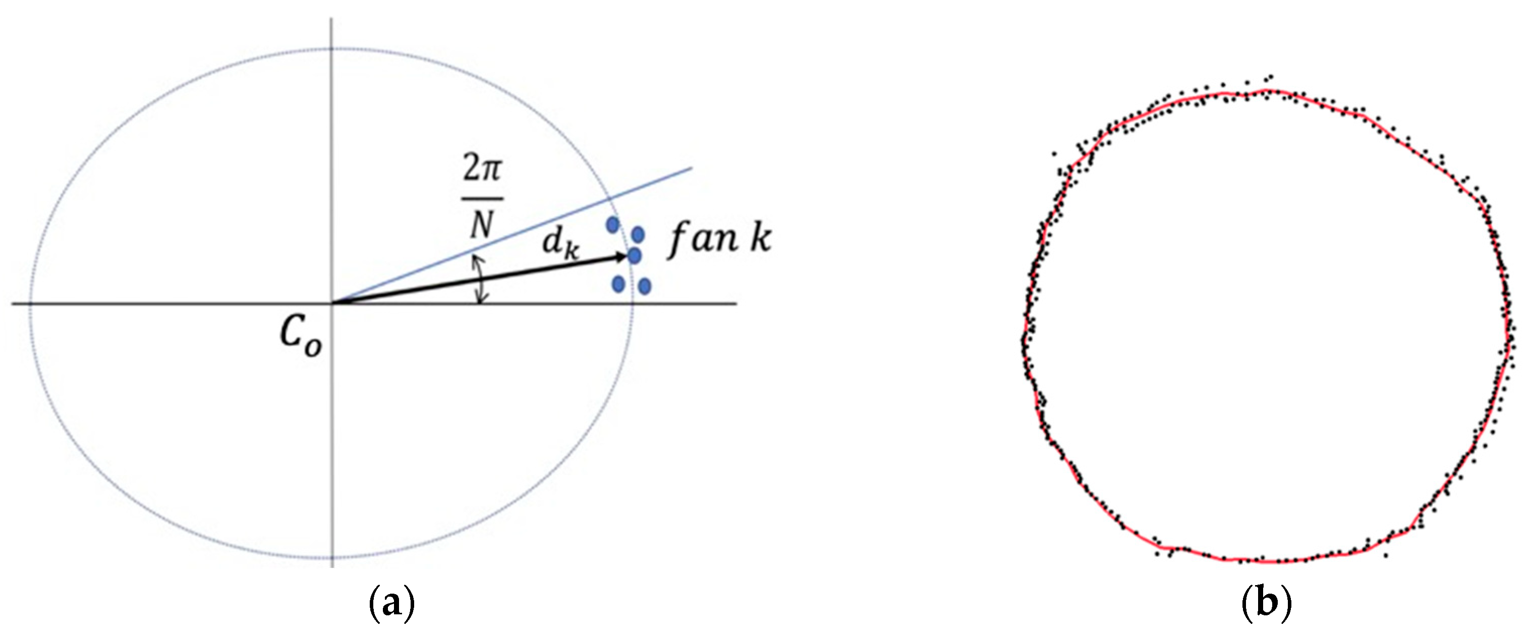
Stem sections are not always well approximated by ellipses. In this study, an N-sided polygon was used to more faithfully approximate the contour shape of a stem section [22]. To calculate an N-sided polygon from noisy points in a stable manner, cross-sectional points are divided into N fans at equal angles, as shown in Figure 12a. The median distance from the center is then calculated in each fan.
Suppose that C o is the center of the closed curve, d k is the median distance in fan k , and h k is the z coordinate of the horizontal plane. Then, the vertex Q k of the polygon can be calculated as:
Q k = C o + ( d k cos ( 2 k 1 ) π N ,   d k sin ( 2 k 1 ) π N ,   h k ) ( k = 1 , , N )
When vertices { Q k }   ( k = 1 , , N ) are calculated in all fan regions, they are connected to generate an N-sided polygon. Figure 12b shows the N-sided polygon of a stem-sectional shape. In this study, the number of vertices of a polygon was set to N = 36.

Spline Curve Approximation

To smoothly interpolate an N-sided polygon as a smooth spline curve, subdivision schemes are useful [22]. In this study, a simple subdivision scheme based on a four-point subdivision scheme was used [24]. Figure 13a shows the four-point subdivision scheme, which doubles the number of vertices of a polygon. In this scheme, { Q j ( k + 1 ) }   ( j = 1 , , 2 n ) are calculated from { Q i ( k ) }   ( i = 1 , 2 , , n ) using the following equation:
{ Q 2 i ( k + 1 ) = Q i ( k )   Q 2 i + 1 ( k + 1 ) = 1 16 Q i 1 ( k ) + 9 16 Q i ( k ) + 9 16 Q i + 1 ( k ) 1 16 Q i + 2 ( k )
By repeatedly applying the subdivision scheme, a smooth spline curve can be generated from an N-sided polygon, as shown in Figure 13b.

2.2.7. Extraction of Stems as Vertically Aligned Curves

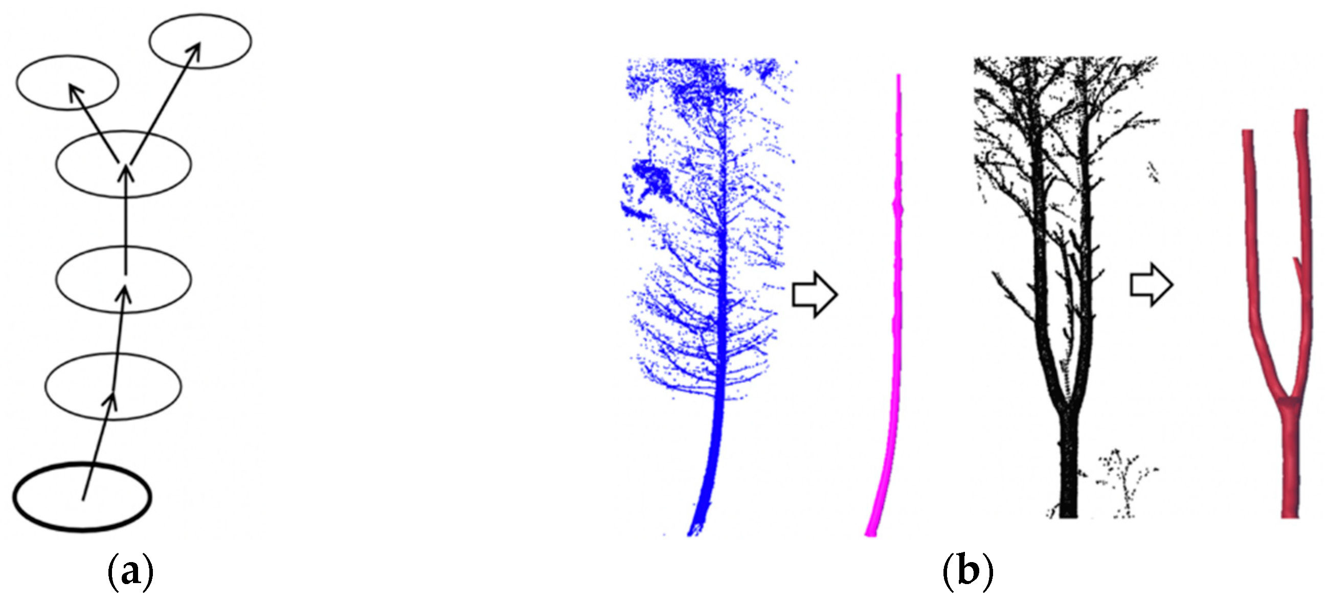
Contour curves of the same stem are placed in the nearly vertical direction, as shown in Figure 11. Therefore, each stem can be extracted as closed curves that are almost vertically placed. Suppose that closed curves C i α and C j β are on the horizontal planes α and ( α β ) . Then, C i α and C j β are regarded as the same stem only if the following conditions are satisfied.
(1)
C i α and C j β are overlapping when they are projected on the horizontal plane.
(2)
The difference between their z coordinates is less than the threshold t z .
(3)
The difference between their radii is less than the threshold t r .
In this study, the threshold t z was set to 0.5 m, and the threshold t r was defined as 10% of the larger radius of C i α and C j β .
By selecting closed curves that satisfy the conditions and sorting them using the z coordinates, each stem shape can be extracted as a set of closed curves, as shown in Figure 14a. The three-dimensional model of each stem can be reconstructed by connecting sectional shapes, as shown in Figure 14b. Our method can be applied to branching stems.

2.2.8. Calculation of Traits

Various stem traits, such as stem curve, DBH, diameter at arbitrary height, section area, and height, can be calculated using closed curves representing a stem shape. Suppose that a stem is represented as a sequence of closed curves { C i }   ( i = 1 , . , n ) .
The center of each closed curve is calculated as the center of gravity. First, the region enclosed by the closed curve C i is triangulated as { T i j } ( j = 1 , . , m ) . The center and the area of triangle T i j are denoted as t i j and s i j , respectively. Then, the area A i and the center Q i of the stem section I are calculated as:
A i = j = 0 m s i j ,   Q i = 1 A i j = 0 m s i j t i j
For the diameters of each stem section, the maximum diameter through the center Q i is calculated from the closed curve. The diameter at a specific height, such as DBH, is calculated by linearly interpolating the diameters of closed curves that are close to the specific height.
To calculate tree height, a bounding circle is calculated, so that all closed curves are enclosed on the horizontal plane, as shown in Figure 15a. Then, an enlarged circle with a radius k times larger than the bounding circle is generated. In this study, k was set to 5. A cylinder can be generated by sweeping the enlarged circle, as shown in Figure 15b. Point cloud files are then reloaded to detect the height range of points contained in each cylinder. The height ranges are regarded as the heights of individual trees.

3. Results

3.1. Experimental Methods

In this study, we developed point processing methods for large-scale point clouds of forest stands. The proposed methods were evaluated using the Datasets A, B, C, and D acquired in Site 1 and 2, as shown in Table 1. First, we evaluated the memory size, computation time, and stem detection rate of the proposed method using Dataset A. Then, we calculated stem diameters and heights using Dataset B and compared them to manual measurements to evaluate their accuracy. We also evaluated the reproducibility of calculated traits using Dataset C and D.
Our system was implemented using C++ and Qt5. The programing code for point processing was developed ourselves. In our experiments, processing time was evaluated as elapsed time on a Linux PC platform with an Intel Core i7 CPU and 64 GB of RAM.

3.2. Evaluation for Processing Large-Scale Point Clouds

3.2.1. Evaluation of Required Memory Size for Large-Scale Point Clouds

In this study, the memory requirements and performance of the proposed method were evaluated using Dataset A, which was measured at 37 locations in Site 1. Table 3 shows the size of the dataset, in which the coordinates and intensity values were represented as 32-bit floating point numbers. In the original point clouds, the number of measurements was 7.0 billion, and the number of valid coordinates was 3.6 billion. Since the data size of each point is 16 byte in binary format, the required RAM is 112 GB for all measurement data and 43 GB for only valid coordinates.
Our method processes one point cloud file at a time and releases the memory space after the calculation. Since each file contains about 200 million pieces of measurement data, the data size in RAM is 3.2 GB. This data size is small enough to be maintained on most PCs.
Then, the data size of the cross-sectional points was evaluated. Figure 16 shows the stems extracted from Dataset A. Cross-sectional points were calculated using horizontal planes with 5-cm and 10-cm intervals. Table 4 shows the number and data size of cross-sectional points. Each section point was represented as (x, y) on each horizontal plane. From 3.6 billion points in Dataset A, the number of cross-sectional points was 39 million at 10-cm intervals, and 79 million at 5-cm intervals. Their data sizes were 313 MB and 632 MB, respectively. When comparing the data sizes to all valid coordinates, the ratios of data sizes were 0.74% at 10 cm intervals and 1.43% at 5 cm intervals. Since the stem representation in this study is small, a number of stems in a large-scale plot can be maintained on a common PC.

3.2.2. Performance of Point Processing

In this study, point cloud files in PTX format were converted into binary files in preprocessing because it is very time-consuming to load ASCII files. The data size of the binary files is about 112GB, as shown in Table 3.
Table 5 shows the calculation time when cross-sectional points were calculated at 10-cm intervals. The elapsed time was 1187 s to detect 1381 stems from Dataset A. In the current implementation, the points on the ground were removed while loading each point cloud file. Therefore, the loading time and ground removal time could not be separated.
In this evaluation, 84% of the computational time was spent on loading and ground removal. It was time consuming to load large-scale point clouds even when point clouds were stored in binary format. On the other hand, the calculation of cross-sectional points, curve fitting, and stem detection took only 186 s.

3.2.3. Detection of Stems

The detection rate of stems was evaluated using 636 target trees at Site 1. In this study, 635 trees were detected at the correct positions from point clouds. The detection rate was 99.8%. The only case of failure was the thinnest tree on the site, with 4.1 cm DBH at 4.7 m height. Since the laser scanner locations were not close to the missed tree, the number of points was not enough to detect the tree.
Our method could achieve a very good result. We consider that there are two main reasons for the high detection rate. One is that our method can handle large-scale point clouds, and therefore we could capture point clouds in the test sites in a high-density mode, such as 200 million measurements. The other reason is that our method resamples points on stems from the wireframe. Therefore, our method is not sensitive to differences in the point density, although the point density on each stem varies with the distance from the laser scanner location.

3.3. Evaluation of Stem Sections

3.3.1. Estimation of Diameter and Height

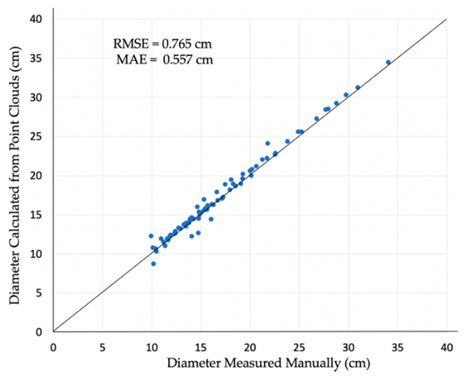
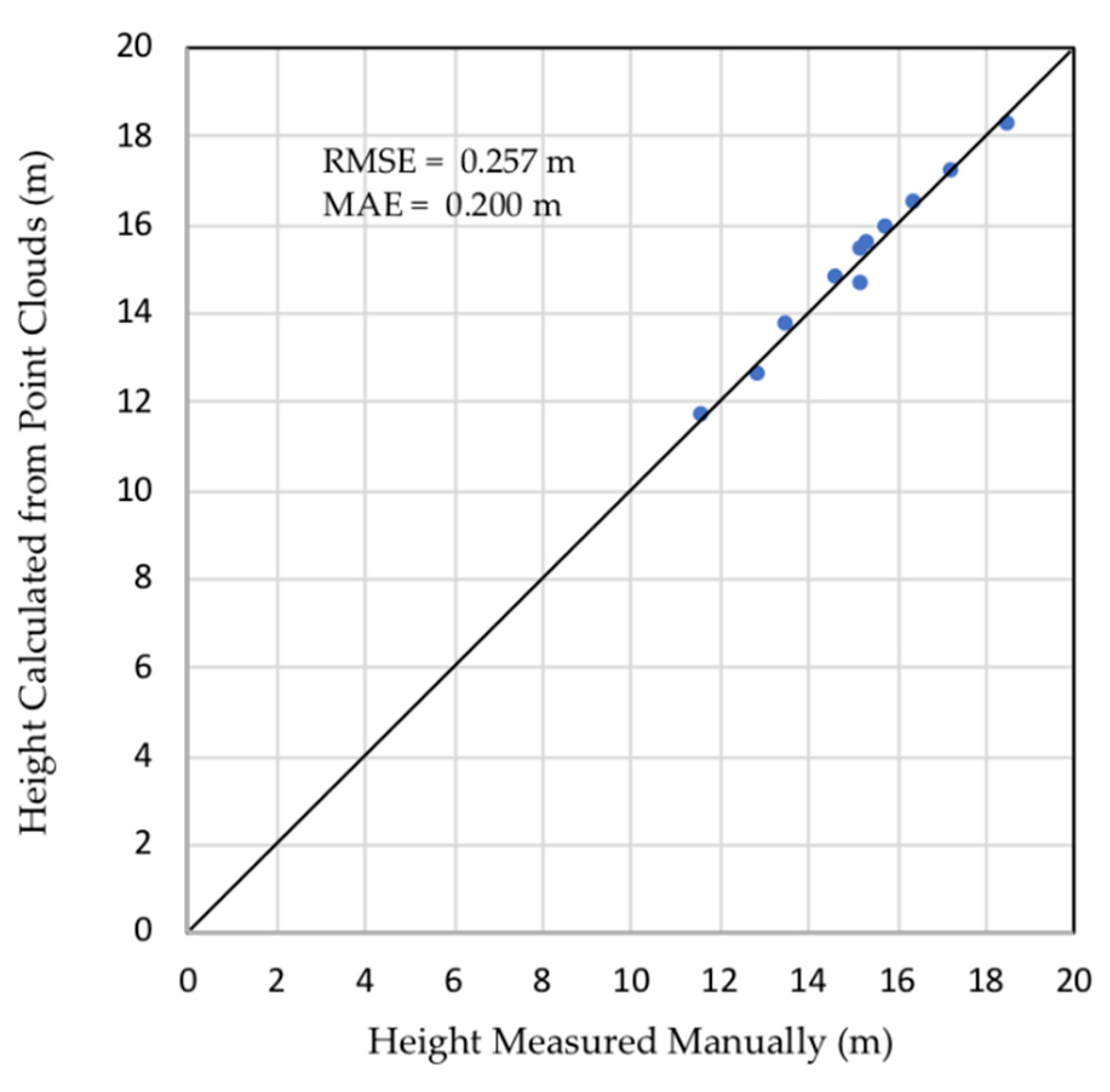
This study evaluated the accuracy of stem diameters at various heights and tree heights using Dataset B. Figure 17 shows a comparison between the manually measured diameters and the diameters calculated from point clouds. In the manual measurement, the diameters were measured from the cross-sectional shapes of 82 disks obtained from eight felled trees. The root mean square error (RMSE) was 0.765 cm, and the mean absolute error (MAE) was 0.557 cm. In this study, the diameters measured from point clouds tended to be slightly larger than the manually measured diameters, as shown in Figure 18. Since this dataset was measured on a windy day, it is considered that this was due to the tree sway caused by the wind. Figure 19 shows a comparison of manually measured and calculated heights of trees in Datasets B and C. The RMSE was 0.275 m, and the MAE was 0.200 m.

3.3.2. Reproducibility of Calculated Traits

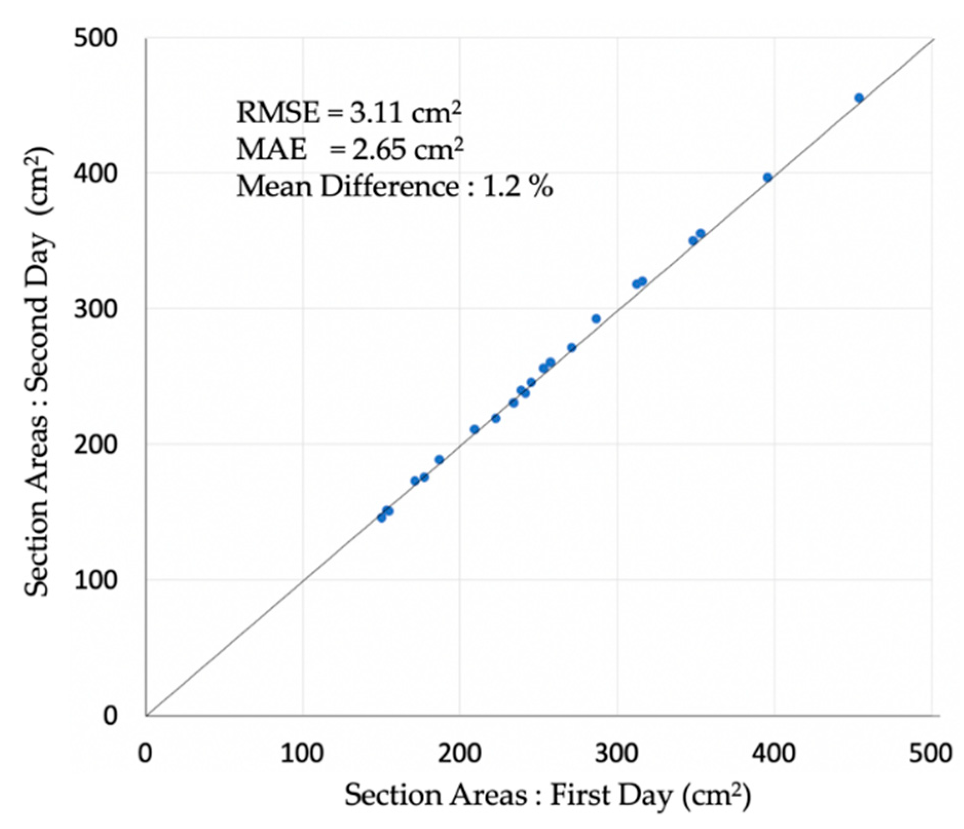
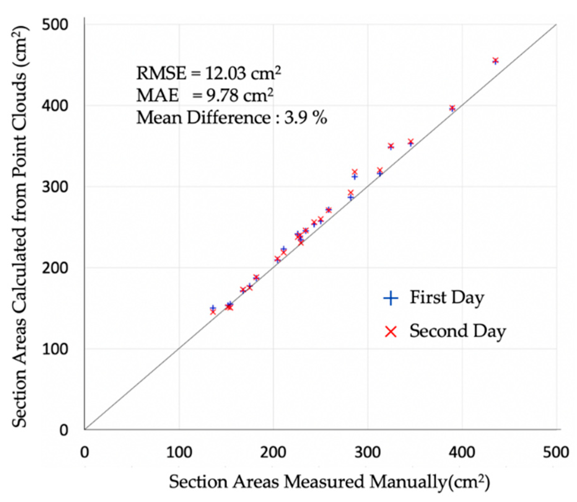
This study evaluated the reproducibility of calculated traits using Datasets C and D, which were measured on different days with different scanner location layouts. There was almost no wind on both days. Figure 20 shows a comparison of section areas calculated from Datasets C and D. The mean difference was 1.2%. The results calculated from the point clouds were highly reproducible. Figure 21 shows a comparison with manual measurement. The mean difference was 3.9%, which was larger than the difference between the two-day measurements.

4. Discussion

4.1. Efficiency of Point Processing

In forest surveys using TLS, point clouds are measured at many locations, and the data size often becomes too large to process on a common PC. In this study, cross-sectional points were calculated in an out-of-core manner using a limited amount of RAM, and various stem traits were calculated from cross-sectional stem points.
For calculating stem sections in our experiments, 7.0 billion measurements were processed in about 20 min. This result indicates that 5.9 million measurements could be processed per second, and therefore, each point cloud with 200 million measurements could be processed in about 34 s. We can conclude that the huge point clouds of a forest stand can be processed in a practical time using the proposed method. We note that the performance would be greatly improved by using a solid-state drive (SSD) instead of a hard disk drive (HDD), because much of the computation time is spent loading large datasets from data storage devices. We also note that a large capacity SSD is required to store forest data. For example, to store the original point clouds of Dataset A, represented in PTX format, 265 GB is required.
Since the proposed method calculates stem traits from cross-sectional points of each stem, a large RAM capacity is not required for processing large-scale point clouds. In our experiments, at 10-cm intervals, the data size of Dataset A could be reduced to 0.73% compared to the original point clouds. This result indicates that the proposed method could be used for conducting a large-scale forest survey. With the advent of TLS, it has become possible to acquire point clouds of forest stands in high resolution and obtain 3D morphological information of each stem composing the forest stands. The processing of huge point cloud data has been a major obstacle in forest measurement applications [25], but we believe that the proposed method can overcome this obstacle.

4.2. Accuracy of Stem Detection and Calculation of Stem Traits

The stem detection rate was 99.8% at Site 1. Only one individual among the 636 target trees was considered a failure because of an insufficient number of points on the stem. This rate is considered to be practically sufficient to estimate the amount of forest resources. This result also suggests that it is important to plan laser scanning locations carefully, so that all target trees can be adequately measured, especially when stems are thin.
The proposed method was highly accurate in estimating stem traits. In particular, this method could accurately estimate stem diameters at arbitrary heights, without destruction of trees. In addition, the experimental results using Datasets C and D showed that stem traits calculated from point clouds were highly reproducible when measured on windless days. On the other hand, considering that the accuracy of Dataset B was slightly deteriorated due to wind sway, it is necessary to measure point clouds under less windy conditions to obtain accurate stem traits with a high accuracy.
In Figure 21, the difference between the two-day measurements was smaller than the difference from the manual measurement. The difference between the manually measured traits and the calculated traits seems to be due to the bias of the measurement methods. In contrast, forest surveys using TLS would be promising as a low-biased measurement.

4.3. Morphological Traits Calculated from Sectional Shapes of Stems

In the proposed method, the complex shapes of stem sections were robustly and accurately approximated as N-sided polygons and spline curves. The sectional shape is considered one of the important morphological traits for comprehending the situation of a forest stand or of individual trees. However, it has previously been difficult to precisely measure such sectional shapes in field investigations without destructive measurements. Cross-sectional shapes of stems are useful for a variety of applications, such as estimation of stem volumes and lumber yields. Additionally, sectional shapes are important factors when evaluating windthrow resistance with respect to stem breakage [26]. The sectional shape or tree-ring shape would indicate radial growth conditions because trees physiologically adjust the rate of cambium cell differentiation to adapt to various external factors, such as environmental stresses and bio-geophysical factors [27].
Stem forms can be reconstructed from stem sectional contours at various heights. By using stem forms, the taper of each stem can be calculated. Stem curvature as an index of straightness of stems can also be obtained using a polyline passing through center positions. By using stem-sectional contours, various stem morphological traits can be analyzed and evaluated for each individual tree in forest stands.
In this study, we focused on stems in forest stands, but we believe that the quantification of other tree parts such as leaves and branches should also be pursued for the better understanding of whole trees and forest stands. Our future challenge is to develop efficient and accurate methods for such organs.

4.4. Application for Forest Investigations

In the proposed method, stem traits are estimated automatically and robustly using standardized procedures. The proposed method is expected to reduce the bias of manual measurements in forest surveys. The proposed method can be applied to forest investigations in various fields of forestry, forest management, and forest science, and can be used for estimating the amount of forest resources and the quantity and quality of individual stems for forestry and for diagnosing the condition of forest stands and individual trees. Additionally, the proposed method would be useful for phenotyping individual trees in the field of forest tree breeding. Surveys in forest tree breeding require, not only measuring a large number of individuals in each test site, but also good accuracy. With the development of technologies for high-throughput sequencing and genotyping for genome-wide markers, genome-wide studies including genome-wide association study and genomic selection can be conducted in forest tree species [28,29]. The proposed study method would enable efficient and precise phenotyping of various stem traits in forest tree breeding.

5. Conclusions

In this paper, a new method for detecting tree stems was proposed by calculating their traits from point clouds obtained using TLS. The experiments in this study indicated that the proposed method could efficiently and precisely extract stems and calculate their traits from large-scale point clouds. Since this method can calculate stem traits in an out-of-core manner, large-scale point clouds can be processed using a common PC with a limited RAM size. The experimental results also showed that the proposed method could process billions of points in a practical time. In addition, the accuracy of stem diameters and areas at various heights and tree heights was evaluated in comparison to manual measurements. It was confirmed that the accuracy was sufficient for practical use in various fields, including forest management and forest research. The study also showed the high reproducibility of stem traits calculated from two different point cloud datasets. We believe that the proposed method can be applied to forest investigations in various fields of forestry, forest management, and forest science.
In future work, we would like to investigate point processing methods for the morphological traits of other tree organs, such as branches and leaves. In addition, we hope that our system will be widely used in the forestry and research community. Currently, our system is in the prototyping phase to evaluate the proposed methods, but we plan to make an executable module of our system available to the public in the near future.

Author Contributions

Conceptualization, H.M. and Y.H.; Data curation, K.S. and S.E.; Funding acquisition, H.M. and Y.H.; Investigation, H.M., Y.H., K.S., S.E., M.M. and M.T.; Methodology, H.M.; Software, H.M., K.S. and S.E.; Writing—original draft, H.M., Y.H., K.S. and S.E.; Writing—review & editing, M.M. and M.T. All authors have read and agreed to the published version of the manuscript.

Funding

This work was supported in part by JSPS KAKENHI Grant Numbers JP15K14763 and JP17K07858 and Management Expenses Grants of The University of Electro-Communications.

Institutional Review Board Statement

Not applicable.

Informed Consent Statement

Not applicable.

Data Availability Statement

Not applicable.

Acknowledgments

We are grateful to the members of the Forest Tree Breeding Center, Forestry and Forest Products Research Institute, for their help with field measurements.

Conflicts of Interest

The authors declare no conflict of interest.

References

  1. Del Río, M.; Bravo, F.; Pando, V.; Sanz, G.; de Grado, R.S. Influence of individual tree and stand attributes in stem straightness in Pinus pinaster Ait. stands. Ann. For. Sci. 2004, 61, 141–148. [Google Scholar] [CrossRef]
  2. Thies, M.; Pfeifer, N.; Winterhalder, D.; Gorte, B.G.H. Three-dimensional reconstruction of stems for assessment of taper, sweep and lean based on laser scanning of standing trees. Scand. J. For. Res. 2004, 19, 571–581. [Google Scholar] [CrossRef]
  3. Wang, D.; Kankare, V.; Puttonen, E.; Hollaus, M.; Pfeifer, N. Reconstructing stem cross section shapes from terrestrial laser scanning. IEEE Geosci. Remote Sens. Lett. 2017, 14, 272–276. [Google Scholar] [CrossRef]
  4. Burt, A.; Disney, M.I.; Calders, K. Extracting individual trees from lidar point clouds using treeseg. Methods Ecol. Evol. 2019, 10, 438–445. [Google Scholar] [CrossRef] [Green Version]
  5. Raumonen, P.; Åkerblom, M.; Kaasalainen, M.; Casella, E.; Calders, K.; Murphy, S. Massive-Scale Tree Modelling from TLS Data. In ISPRS Annals of Photogrammetry, Remote Sensing & Spatial Information Sciences, Proceedings of the PIA15+HRIGI15—Joint ISPRS Conference, Munich, Germany, 25–27 March 2015; International Society for Photogrammetry and Remote Sensing: Hannover, Germany, 2015; Volume II-3/W, pp. 189–196. [Google Scholar]
  6. Olofsson, K.; Holmgren, J. Single tree stem profile detection using terrestrial laser scanner data, flatness saliency features and curvature properties. Forests 2016, 7, 207. [Google Scholar] [CrossRef]
  7. Zhang, W.; Wan, P.; Wang, T.; Cai, S.; Chen, Y.; Jin, X.; Yan, G. A novel approach for the detection of standing tree stems from plot-level terrestrial laser scanning data. Remote Sens. 2019, 11, 211. [Google Scholar] [CrossRef] [Green Version]
  8. Lefsky, M.; McHale, M. Volume estimates of trees with complex architecture from terrestrial laser scan. J. Appl. Remote Sens. 2008, 2, 023521. [Google Scholar]
  9. Wang, D.; Hollaus, M.; Puttonen, E.; Pfeifer, N. Automatic and self-adaptive stem reconstruction in landslide-affected forests. Remote Sens. 2016, 8, 974. [Google Scholar] [CrossRef] [Green Version]
  10. Puttonen, E.; Lehtomäki, M.; Kaartinen, H.; Zhu, L.; Kukko, A.; Jaakkola, A. Improved sampling for terrestrial and mobile laser scanner point cloud data. Remote Sens. 2013, 5, 1754–1773. [Google Scholar] [CrossRef] [Green Version]
  11. Simonse, M.; Aschoff, T.; Spiecker, H.; Thies, M. Automatic determination of forest inventory parameters using terrestrial laserscanning. In Proceedings of the ScandLaser Scientific Workshop on Airborne Laser Scanning of Forest, Umea, Sweden, 3–4 September 2003; Volume 2003, pp. 252–258. [Google Scholar]
  12. Rabbani, T.; Van Den Heuvel, F. Efficient hough transform for automatic detection of cylinders in point clouds. ISPRS WG 2005, 3, 60–65. [Google Scholar]
  13. Olofsson, K.; Holmgren, J.; Olsson, H. Tree stem and height measurements using terrestrial laser scanning and the RANSAC algorithm. Remote Sens. 2014, 6, 4323–4344. [Google Scholar] [CrossRef] [Green Version]
  14. Lindberg, E.; Holmgren, J.; Olofsson, K.; Olsson, H. Estimation of stem attributes using a combination of terrestrial and airborne laser scanning. Eur. J. For. Res. 2012, 131, 1917–1931. [Google Scholar] [CrossRef] [Green Version]
  15. Gorte, B.; Pfeifer, N. Structuring laser-scanned trees using 3D mathematical morphology. Int. Arch. Photogramm. Remote Sens. 2004, 35, 929–933. [Google Scholar]
  16. Schnabel, R.; Wahl, R.; Klein, R. Efficient RANSAC for point-cloud shape detection. In Computer Graphics Forum; Blackwell Publishing Ltd.: Oxford, UK, 2007; Volume 26, pp. 214–226. [Google Scholar]
  17. Gorte, B.; Winterhalder, D. Reconstruction of laser-scanned trees using filter operations in the 3d raster domain. Remote Sens. Spat. Inf. Sci. 2012, 36, W2. [Google Scholar]
  18. Vonderach, C.; Voegtle, T.; Adler, P. Voxel-based approach for estimating urban tree volume from terrestrial laser scanning data. In ISPRS International Archives of the Photogrammetry, Remote Sensing and Spatial Information Science, Proceedings of the XXII ISPRS Congress, Melbourne, Australia, 25 August–1 September 2012; International Society for Photogrammetry and Remote Sensing: Hannover, Germany, 2012; Volume XXXIX-B8, pp. 451–456. [Google Scholar]
  19. Aschoff, T.; Thies, M.; Spiecker, H. Describing forest stands using terrestrial laser-scanning. In ISPRS International Archives of Photogrammetry, Remote Sensing and Spatial Information Sciences, Proceedings of Istanbul 20th ISPRS World Congress, Istanbul, Turkey 12–23 July 2004; International Society for Photogrammetry and Remote Sensing: Hannover, Germany, 2004; Volume XXXV, Part B; pp. 237–241. [Google Scholar]
  20. Saito, K.; Masuda, H.; Hiraoka, Y.; Matsushita, M.; Takahashi, M. Shape reconstruction of trees in massive-scale forests for evaluation of morphological traits. In Proceedings of the SilviLaser, Blacksburg, VA, USA, 10–12 October 2017; p. 166. [Google Scholar]
  21. Pfeifer, N.; Winterhalder, D. Modelling of tree cross sections from terrestrial laser scanning data with free-form curves. Int. Arch. Photogram. Remote Sens. Spat. Inf. Sci. 2004, 36, 76–81. [Google Scholar]
  22. Eto, S.; Masuda, H.; Hiraoka, Y.; Matsushita, M.; Takahashi, M. Extraction and evaluation of tree traits using TLS point cloud. Int. Arch. Photogramm. Remote Sens. Spatial Inf. Sci. 2020, XLIII-B2-2020, 205–210. [Google Scholar] [CrossRef]
  23. Masuda, H.; Niwa, T.; Tanaka, I.; Matsuoka, R. Reconstruction of polygonal faces from large-scale point-clouds of engineering plants. Comput. Aided Des. Appl. 2015, 12, 555–563. [Google Scholar] [CrossRef]
  24. Dyn, N. Subdivision schemes in CAGD. Adv. Numer. Anal. 1992, 2, 36–104. [Google Scholar]
  25. Kato, A.; Ishii, H.; Enoki, T.; Osawa, A.; Kobayashi, T.; Umeki, K.; Sasaki, T.; Matsue, K. Application of laser remote sensing to forest ecological research. J. Jpn. For. Soc. 2014, 96, 168–181. [Google Scholar] [CrossRef] [Green Version]
  26. Koizumi, A.; Ikeda, K.; Sawata, K.; Hirai, T. Nondestructive measurement of cross-sectional shape of a tree trunk. J. Wood Sci. 2011, 57, 276–281. [Google Scholar] [CrossRef] [Green Version]
  27. Shi, P.-J.; Huang, J.-G.; Hui, C.; Grissino-Mayer, H.D.; Tardif, J.C.; Zhai, L.-H.; Wang, F.-S.; Li, B.-L. Capturing spiral radial growth of conifers using the superellipse to model tree-ring geometric shape. Front. Plant Sci. 2015, 6, 856. [Google Scholar] [CrossRef] [PubMed] [Green Version]
  28. Hiraoka, Y.; Fukatsu, E.; Mishima, K.; Hirao, T.; Teshima, K.M.; Tamura, M.; Tsubomura, M.; Iki, T.; Kurita, M.; Takahashi, M.; et al. Potential of genome-wide studies in unrelated plus trees of a coniferous species. Cryptomeria japonica (Japanese cedar). Front. Plant Sci. 2018, 9, 1322. [Google Scholar] [CrossRef] [PubMed]
  29. Nagano, S.; Hirao, T.; Takashima, Y.; Matsushita, M.; Mishima, K.; Takahashi, M.; Iki, T.; Ishiguri, F.; Hiraoka, H. SNP genotyping with target amplicon sequencing using a multiplexed primer panel and its application to genomic prediction in Japanese Cedar, Cryptomeria japonica (L.f.) D.Don. Forests 2020, 11, 898. [Google Scholar] [CrossRef]
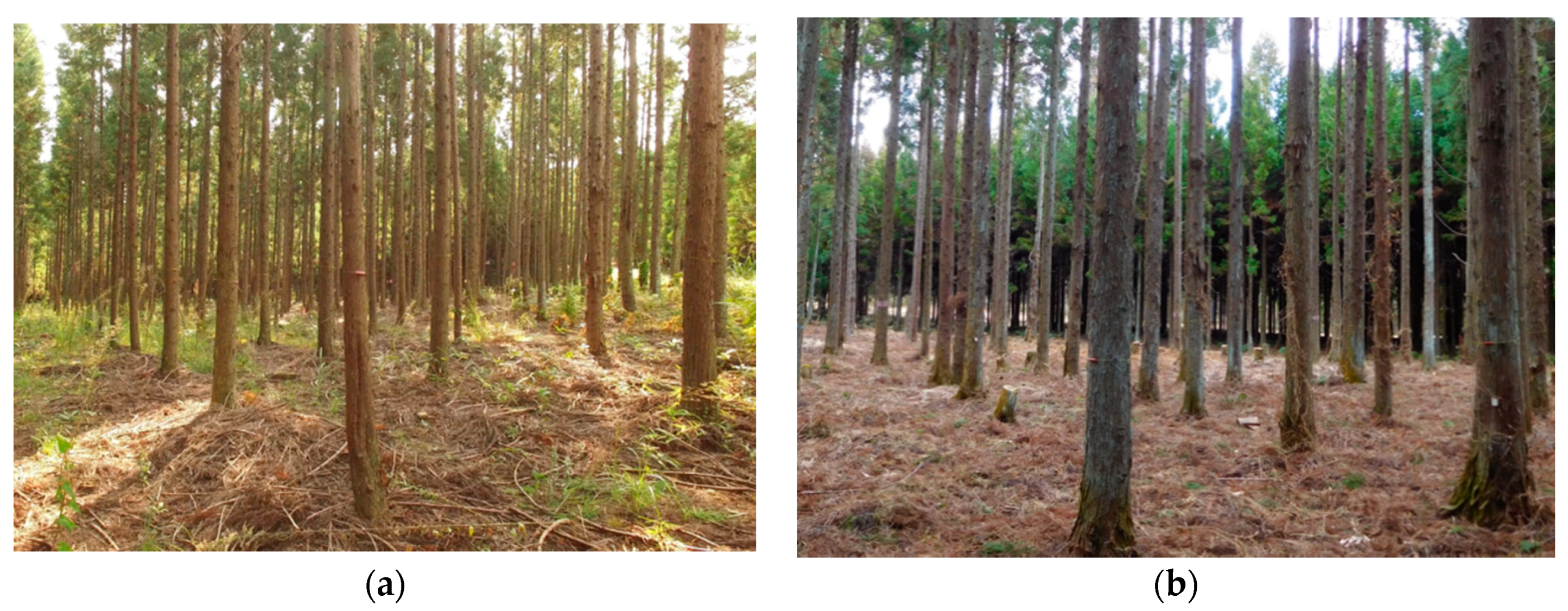
Figure 1. Pictures of the study sites. (a) Site 1; (b) Site 2.
Remotesensing 13 02476 g001
Figure 2. Contour curves of stem sections.
Remotesensing 13 02476 g002
Figure 3. Process outline.
Remotesensing 13 02476 g003
Figure 4. Measurement by TLS. (a) Conceptual diagram of TLS measurement; (b) Example of a point cloud with a two-dimensional lattice structure.
Remotesensing 13 02476 g004
Figure 5. Removal of points on the ground. (a) Example of a point cloud in a test site; (b) digital terrain model (DTM); (c) points of trees after removing ones on the ground (navy blue).
Remotesensing 13 02476 g005
Figure 6. Generating a wireframe model. (a) Estimation of the distance between neighbor points; (b) edges between neighboring points (a wireframe model).
Remotesensing 13 02476 g006
Figure 7. Segmentation into connected regions. (a) Connected regions; (b) removal of small regions.
Remotesensing 13 02476 g007
Figure 8. Section points between a wireframe model and horizontal planes. (a) Horizontal planes; (b) intersections (white circle); (c) section points.
Remotesensing 13 02476 g008
Figure 9. Section points merged on each horizontal plane.
Remotesensing 13 02476 g009
Figure 10. Segmentation of cross-sectional points. (a) Section points; (b) Delaunay triangulation; (c) connected components as stem section candidates.
Remotesensing 13 02476 g010
Figure 11. Ellipses detected from point-clouds.
Remotesensing 13 02476 g011
Figure 12. Detailed sectional shape of a stem. (a) Median distance in a fan; (b) N-sided polygon of a stem sectional shape.
Remotesensing 13 02476 g012
Figure 13. Stem representation using spline curve. (a) Four-point subdivision scheme; (b) interpolation by subdivision scheme.
Remotesensing 13 02476 g013
Figure 14. Extraction of each stem from stem sections. (a) Overlapping closed curves; (b) reconstruction of stem shapes.
Remotesensing 13 02476 g014
Figure 15. Calculation of tree height. (a) Circle on the horizontal plane; (b) points in a cylinder.
Remotesensing 13 02476 g015
Figure 16. Stems extracted from the dataset of Site 1.
Remotesensing 13 02476 g016
Figure 17. Comparison of manually-measured and calculated diameters.
Remotesensing 13 02476 g017
Figure 18. Diameters of stem sections of a sample tree.
Remotesensing 13 02476 g018
Figure 19. Comparison of manually-measured and calculated heights.
Remotesensing 13 02476 g019
Figure 20. Estimation of section areas.
Remotesensing 13 02476 g020
Figure 21. Comparison of measured and calculated section areas.
Remotesensing 13 02476 g021
Table 1. Summary of three studies conducted at Site 1 and Site 2.
Study 1Study 2Study 3
DatasetABCD
Study siteSite 1Site 2Site 2Site 2
Measured age (years)18222323
Objective area (ha)0.5170.0560.0190.018
Stem density within
Objective area (ha−1)
1410123814401598
Number of targeted trees636833
Scanner typeS120X330X330X330
Number of scanner locations37191215
Number of points3,573,945,6161,237,481,441867,906,4021,105,273,190
Table 2. Specifications and settings of laser scanners.
FARO Focus3D S120FARO Focus3D X330
Range of distance0.6–120 m0.6–330 m
Wave length905 nm1550 nm
Ranging error±2 mm at 10 m and 25 m, each at 90% and 10% reflectivity
Angle resolution0.018 deg (20,480 measurements per 360 deg)
Scan speed488,000 points/sec (Quality 2X)
Table 3. Data size of Dataset A.
Number of measurements 7.0 billion
Data size112 GB
Number of valid points3.6 billion
Data size43 GB
Table 4. The number and data size of section points obtained from Dataset A.
Interval of Sections
10 cm5 cm
Number of section points39 million79 million
Data size313 MB632 MB
Ratio to original coordinate data0.73%1.47%
Number of section curves62,624131,458
Table 5. Timing for stem detection from Dataset A using 10-cm intervals.
TimeRatio
Loading and ground removal1001 s84%
Calculation of cross-sectional points45 s3%
Curve fitting121 s10%
Stem detection20 s2%
Total1187 s100%
Publisher’s Note: MDPI stays neutral with regard to jurisdictional claims in published maps and institutional affiliations.