Spectral Characteristics of the Antarctic Vegetation: A Case Study of Barton Peninsula

Abstract

Spectral information is a proxy for understanding the characteristics of ground targets without a potentially disruptive contact. A spectral library is a collection of this information and serves as reference data in remote sensing analyses. Although widely used, data of this type for most ground objects in polar regions are notably absent. Remote sensing data are widely used in polar research because they can provide helpful information for difficult-to-access or extensive areas. However, a lack of ground truth hinders remote sensing efforts. Accordingly, a spectral library was developed for 16 common vegetation species and decayed moss in the ice-free areas of Antarctica using a field spectrometer. In particular, the relative importance of shortwave infrared wavelengths in identifying Antarctic vegetation using spectral similarity comparisons was demonstrated. Due to the lack of available remote sensing images of the study area, simulated images were generated using the developed spectral library. Then, these images were used to evaluate the potential performance of the classification and spectral unmixing according to spectral resolution. We believe that the developed library will enhance our understanding of Antarctic vegetation and will assist in the analysis of various remote sensing data.

1. Introduction

Recent interest in climate change and global warming has affected the distribution and function of vegetation by changing the environmental conditions of ecosystems [1]. Since the Antarctic ecosystem is particularly sensitive to environmental change, studying its responses can enhance our understanding of such changes [2,3,4,5,6]. The monitoring of terrestrial biodiversity in the Antarctic Peninsula and the South Shetland Islands, which are some of the most rapidly warming areas in the world [6,7], is vital as a proxy for climate change.

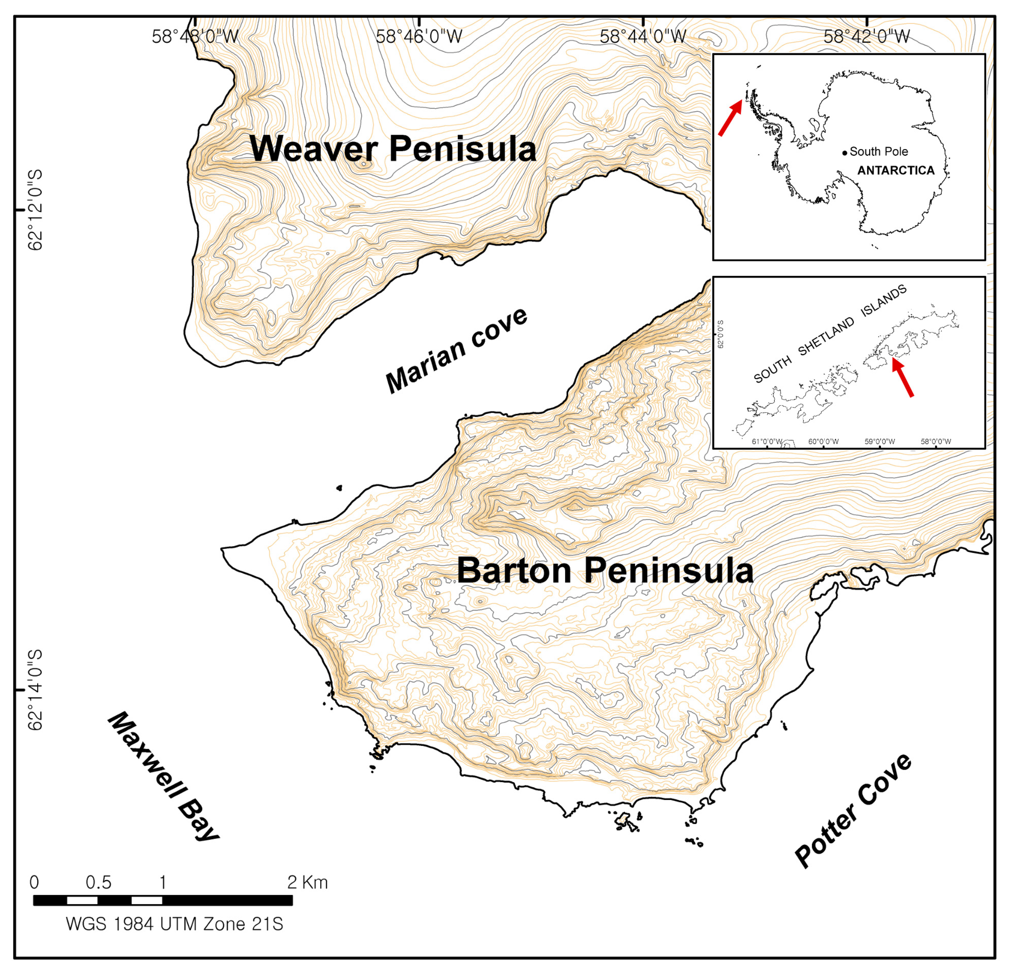
Detailed information on the maritime biodiversity in Antarctica has been collected via field surveys, but this information is limited to the areas most frequently visited by researchers, primarily near Antarctic research stations. Therefore, on King George Island, the largest of the South Shetland Islands and the most concentrated region of Antarctic research stations, various biodiversity monitoring studies via field surveys have been conducted. In the Maxwell Bay area of King George Island, vegetation cover was surveyed [8], and the species density of bryophytes and lichens was calculated for the Barton Peninsula around King Sejong Station [9]. Due to the extreme environmental conditions, only two species of flowering plants, Deschampsia antarctica and Colobanthus quitensis, grow in small and sparse patches; however, cryptogamic species, including 33 bryophytes (mosses) and 62 lichens, are dominant in most snow-free regions [8,9]. Changes in the lichen community diversity and composition of a deglaciated gradient were analyzed using five 50 × 50 cm grids at 24 sites in the Potter Peninsula [10]. The present study reports that the patterns of these Antarctic lichen communities are dynamic and highly heterogeneous due to a strong influence of microsite factors and macroclimate variables. In Admiralty Bay, biomass and net annual production patterns were analyzed for four moss species in Antarctica [11], and the driving mechanisms of vegetation, including soil characteristics and landscape elements (altitude and geomorphological variations), were investigated [12] in the surrounding area of Arctowski Station. A distribution map was generated for 35 vegetation communities of the Keller Peninsula [13], and the lichen biota dynamics of Lions Rump for the past 20 years were characterized, showing that the most significant changes had taken place in the forefield of a glacier and on the young moraines [14]. In addition, the distributions of the representative flowering plant Deschampsia antarctica [15] and of mosses [16] were surveyed and compared between the South Shetland Islands and the Antarctic Peninsula.

However, periodic field surveys of extended areas are financially and physically costly, and the human activity can potentially destroy or disturb the ecosystem. Additionally, survey-based approaches maintain inherent uncertainty when quantifying vegetation cover and variations over relatively long time periods. As an alternative, remote sensing techniques are widely used to periodically monitor quantitative and qualitative states of extensive and/or inaccessible regions. Several studies have been conducted to assess polar vegetational biodiversity using remote sensing approaches over the past decade. Théau et al. [17] used a classification method and spectral mixture analysis for mapping several types of lichen over Northern Quebec using Landsat imagery. They acquired field data using a helicopter and determined the types and percent of coverage by visual inspection. Large-scale mapping analyses using the normalized difference vegetation index (NDVI) from medium-resolution Landsat [18] and SPOT [19] images have been conducted; however, detailed information from these studies is not available due to the limited spatial and spectral resolution of the images and ground truthing efforts. Nonetheless, such research has suggested that a combination of remote sensing data and techniques could potentially help obtain information. Shin et al. [20] used a spectral mixture analysis technique to quantify vegetation abundance at the sub-pixel level from high-resolution KOMPSAT-2 (Korea Multi-Purpose Satellite-2) and QuickBird images of the Barton Peninsula; however, they employed image-driven endmembers instead of field spectra. Liu and Treitz [21] used ground-based near-infrared (NIR) images to develop a vegetation cover model for the Canadian High Arctic, and then applied this model to high-resolution satellite images to examine the spatio-temporal patterns of the vegetation cover over the extended areas. Sun et al. [22] investigated vegetation abundance and health mapping from WorldView-2 data using spectral mixture analysis in the Fildes Peninsula and Ardley Island, King George Island. They categorized mosses and lichens according to their associated health conditions and acquired reference field spectra over approximately 300–1000 nm for large sampling plots (2 m × 2 m), which are suitable for obtaining high resolution satellite data. Accordingly, past vegetation mapping studies of remote sensing data have focused on the analysis of vegetation/spectral indices and on the classification/unmixing of a few vegetation species or conditions due to the relative lack of spectral information and images of the Arctic/Antarctic vegetation.

Incorporating the field spectra of the target areas into the remote sensing analyses can greatly assist with the assessments of inaccessible areas. A spectral library is a set of digital reflectance spectra measured in the laboratory or the field, or remotely by air or spacecraft. They are employed to support imaging spectroscopy studies of the Earth and other planets and include informative wavelength data of both natural and artificial surfaces, such as rocks, minerals, soils, vegetation, snow, and ice [23]. A spectral library can play an important role in identifying the components of unknown targets and quantifying their abundance in mixed pixels. Widely used spectral libraries are contributed to by the Advanced Spaceborne Thermal Emission Reflection Radiometer (ASTER), the NASA Jet Propulsion Laboratory (JPL), the Johns Hopkins University, and the United States Geological Survey (USGS). However, these spectral libraries have been primarily developed for use in mid-latitudinal regions. As the landscapes of the polar regions are quite different, the current libraries may not be applicable for interpreting the ecosystems and landcover types in the Antarctic region. Limited research has been aimed at developing a spectral library of polar vegetation. Goswami and Matharasi [24] developed a vegetation spectral library for the Arctic, Antarctic, and Chihuahuan Desert regions using a hand-held portable spectrometer in the visible and NIR (VNIR) wavelength range. Calvino-Cancela and Martin-Herreroin [25] developed a spectral library for 13 representative moss and lichen species in the Barton Peninsula in the VNIR wavelength range (380–1000 nm). Their classified field-measured spectra showed high overall accuracy in principal component analysis–linear discriminant analysis. However, the analysis also concluded that some species, such as Deschampsia and Prasiola, were challenging to discriminate using their library spectra.

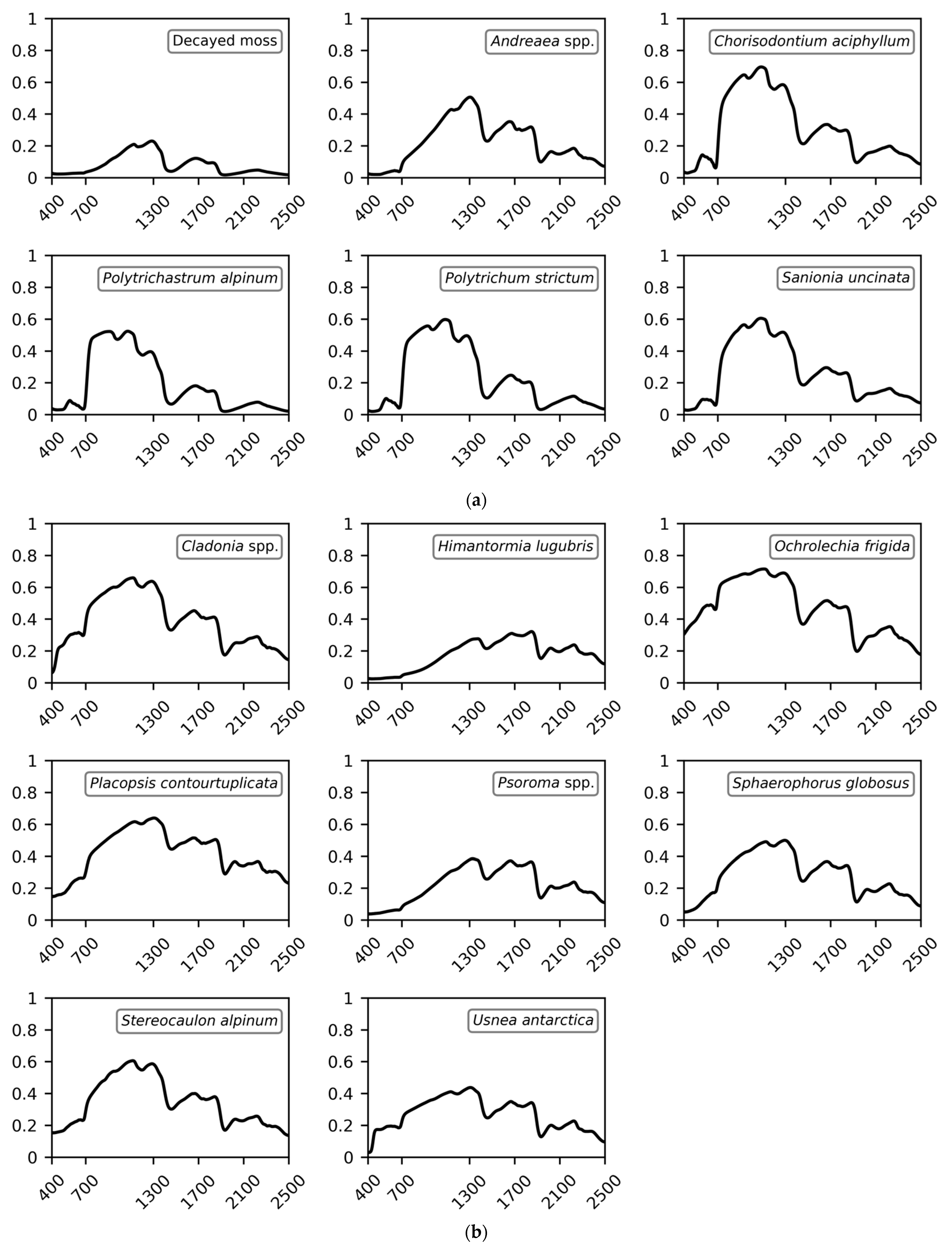
Although the spectral library is crucial for quantitative remote sensing analysis, particularly for inaccessible or difficult-to-access locations such as the polar regions, limited spectral information for ground objects in the polar regions is available. This study had two research goals: (1) the development of a spectral library for Antarctic vegetation; and (2) the investigation of the spectral characteristics of Antarctic vegetation to determine which spectral ranges are the most effective for identifying Antarctic vegetation in remote sensing data. To this end, we first developed a spectral library for 16 representative vegetation species and decayed moss, including mosses, lichens, vascular plants, and one alga often discovered in the ice-free areas of Antarctica. Iterative field spectral data across the visible–shortwave-infrared (SWIR) range (400–2500 nm) were collected for homogeneous vegetation patches and then compiled to generate representative spectra. Both spectrometers and hyperspectral imaging sensors typically use the VNIR (400–1000 nm), SWIR (1000–2500 nm), or full-spectrum (i.e., VNIR–SWIR; 400–2500 nm) ranges. As VNIR sensors are lighter, cheaper, and have a better signal-to-noise ratio than SWIR or full-spectrum sensors, using a VNIR spectrometer or integrating a VNIR imaging sensor to a small unmanned aerial vehicle (UAV) has fewer technical challenges. Therefore, along with developing a spectral library of the Antarctic vegetation species over a full-spectral range, analyses were carried out using spectral discrimination measures to observe the spectral characteristics and potential separability of the Antarctic vegetation by wavelength range. Since sufficient remote sensing images with corresponding surveyed data over the study area are unavailable, artificial images were created and modeled using the developed spectral library, field information, and spectral response functions of widely used remote imaging sensors. The potential performance of the vegetation discrimination was then evaluated for practical classification and unmixing tasks. In particular, we addressed the importance of SWIR wavelengths in discriminating or quantifying Antarctic vegetation species effectively.

2. Materials and Methods

2.1. Study Area

The Barton Peninsula is located between 62.12°S and 62.14°S and 58.42°W and 58.48°W in the southwest of King George Island, the largest of the South Shetland Islands (Figure 1). The elevation of the peninsula ranges only from 0 to 266 m, but the topography is complex [26]. A large part of the ground area is covered with snow throughout the year; however, during the summer, ~12 km² of the regions near the coastal area are snow-free. Soils generally lack nutrients and organic matter, except near seabird nesting sites and penguin rookeries [27]. The climate is relatively warmer, more humid, and milder than that of continental Antarctica, as is more typical of the polar oceanic climate. Based on meteorological records from the Korean Antarctic King Sejong Station in the Barton Peninsula, the annual mean values for this region are: −1.6 °C surface air temperature, 89% relative humidity, and wind speeds of 8.0 m·s⁻¹ [28].

2.2. Measurement of Vegetation Spectra

Surface features have unique signals similar to fingerprints, one of the most well-known biometrics for human identification due to their uniqueness and consistency over time, referred to as spectral reflectance. Different surface objects reflect and absorb electromagnetic radiations in different ways according to their physical and chemical states. Spectral reflectance is a measure of how much energy a surface reflects at a specific wavelength [29]. Generally, in the field procedures employed to acquire reflectance spectra, the flux reflected from a level reflectance reference surface such as a Spectralon panel is first measured, and then the flux reflected from the subject (e.g., vegetation species in this study) is measured. In this study, an ASD Fieldspec 4 spectrometer (Malvern Panalytical Ltd., Malvern, UK) was used to collect field spectra across the 350 to 2500 nm wavelength range at a spectral resolution of 1 nm. Due to the high and fast-changing cloud cover over the study area, the spectra were measured with a contact probe, which had a stable halogen krypton light source attached to the mount of the optic cable. The light source of the contact probe was aligned at a fixed illumination zenith of 23° to the probe body to minimize issues of variable illumination from the surface topography, thereby allowing for the rapid acquisition of spectra at any time of day. The optical cable of the spectrometer was mounted to the contact probe at a fixed view zenith angle of 35° in the same azimuth of the probe axis as the light source [30].

Field campaigns were carried out in selected areas of the Barton Peninsula in the Antarctic summer season, from 17 January to 14 February 2019. As there were no rain or snow events before the acquisition of the field spectra, the impact of water content was minimized.

Table 1. Scientific names and descriptions of the 16 representative vegetation species in Barton Peninsula [9].

Species	Description
Mosses
Andreaea spp.	Very common and dominant on dry, exposed rocks, boulders on stony ground, rock ledges, and outcrops. Sometimes encrusted with epiphytic lichens and mixed with the liverwort Herzogobryum teres.
Chorisodontium aciphyllum (Hook. f. and Wils.), Broth	Turf-forming species occurring almost exclusively on the small Ardley Island near the Fildes Peninsula.
Polytrichastrum alpinum (Hedw.) G.L. Sm.	Small patches associated with Sanionia georgico-uncinata and the grass Deschampsia antarctica and present in fairly moist places near ponds.
Polytrichum strictum Brid.	Small turfs present, with tall turfs being rare on King George Island.
Sanionia uncinata (Hedw.) Loeske	Dominant species distributed primarily on the lower-level terrain in both sheltered and open habitats. Commonly associated with P. alpinum, Bryum spp., and Andreaea spp.
Lichens
Cladonia spp.	Fruticose lichens; commonly associated with turf-forming species C. aciphyllum and P. strictum in the mixed stands.
Himantormia lugubris (Hue.) I.M. Lamb	Fruticose lichens that dominate the lichen community along with U. antarctica.
Ochrolechia frigida (Sw.) Lynge	Commonly associated with S. uncinata and turf-forming mosses on dry habitats and gentle slopes, and nearly absent in wet habitats.
Placopsis contourtuplicata I.M. Lamb	Found on dry and fairly exposed gravels of gentle slopes, forming a rich understory beneath the macrolichens.
Psoroma spp.	Squamulose lichen, usually associated with mosses.
Sphaerophorus globosus (Huds.) Vain.	Fruticose lichens; usually associated with turf-forming species C. aciphyllum and P. strictum in mixed stands.
Stereocaulon alpinum Laurer	Fruticose lichens; growing in dry and exposed areas.
Usnea antarctica Du Rietz	Fruticose lichens; abundant in most habitats from sheltered to very exposed and moist to dry, and showing a tendency to occur in areas with early exposure from snowmelt and in higher altitude locations.
Flowering plants
Colobanthus quitensis (Kunth) Bartl.	Dicot species observed in sheltered areas facing Marian Cove; expanded rapidly and primarily associated with patches of S. uncinata within the Usnea-crustose community.
Deschampsia antarctica Desv.	Monocot species mostly growing in the flat areas used by skuas as resting places around Sejong Point near ponds. Most grass patches were formed in stable, well-drained areas covered by an S. uncinata moss carpet.
Alga
Prasiola crispa (Ligtf.) Kütz. subsp. antarcica (Kütz.) Knebel	Nitrophilous alga; present around ponds near King Sejong Station and penguin rookeries with high nitrogen levels.

displays the scientific names and descriptions of species surveyed in this study. Decayed moss was often observed as mixed or next to other living vegetation in the study area, and we thought it was one of the major components of the ground surface of this area. However, it was difficult to distinguish spectral differences between types of decayed moss. Since the homogeneous and pure targets for 16 vegetation species and decayed moss were first localized to within the field of view, there were mostly no mixed signals in the selected targets. At least 20 individual patches per species were selected, and ten iterative measurements were conducted for each patch. The size of each patch depended on species type and field conditions, but it was a minimum of 5 cm × 5 cm. Spectra for each patch were acquired on different days and at different locations in the Barton Peninsula during the field campaign period. ASD Fieldspec 4 consists of three spectral detectors (relative to the 350–1000 nm, 1001–1800 nm, and 1801–2500 nm wavelength ranges) to capture the full spectral range. The measured spectra often exhibited spectral discontinuities at the borders between these three ranges owing to insufficient sensor warm-up and inhomogeneities of the targets within the field of view [31,32]. These inter-channel radiometric steps were corrected using a radiometric inter-channel jump correction method [31]. To build a spectral library, the reflectance spectra of the 16 species and decayed moss were averaged, with the exclusion of all abnormal spectra and noisy data, across the 350 to 400 nm wavelength range.

2.3. Spectral Similarity Measures between Library Spectra

Various similarity metrics have been developed to quantitatively compare reflectance spectra [33,34]. Spectral correlation (SC) is a derivative of the Pearson’s correlation coefficient (PCC) between the two spectra $x={\left(x_1,x_2,\cdots ,x_n\right)}^{\mathrm{T}}$ and $y={\left(y_1,y_2,\cdots ,y_n\right)}^{\mathrm{T}}$, according to Equation (1) [35]:

$$\mathrm{SC}=\frac{n{{\displaystyle \sum }}_1^n{x}_i{y}_i-{{\displaystyle \sum }}_1^n{x}_i{{\displaystyle \sum }}_1^n{y}_i}{\sqrt{[n{{\displaystyle \sum }}_1^n{x}_i^2-{\left({{\displaystyle \sum }}_1^n{x}_i\right)}^2]\left[n{{\displaystyle \sum }}_1^n{y}_j^2-{\left({{\displaystyle \sum }}_1^n{y}_j\right)}^2\right]}}$$

(1)

where n is the number of spectral bands. SC is relatively simple to compute and considers the overall spectrum shape. The correlation value ranges between −1 and 1 and shows the extent of the linear relationship between the two spectra. SC can be expressed as an angle, applying the arc-cosine.

The spectral angle (SA) is the most widely used spectral similarity index in the analysis of hyperspectral remote sensing imagery. It is similar to the PCC except for the standardization of the data themselves. It measures the angle between two spectral signatures, according to Equation (2) [36]:

$$\mathrm{SA}={\cos }^{-1}\left(\frac{{{\displaystyle \sum }}_1^n{x}_i{y}_i}{\sqrt{{{\displaystyle \sum }}_1^n{x}_i^2}\sqrt{{{\displaystyle \sum }}_1^n{y}_i^2}}\right)$$

(2)

SA analysis yields similar results to Euclidean distance (ED) analysis, but the ED is affected by the brightness temperature of the spectra, while the SA and SC are invariant to brightness.

Another common metric is the spectral information divergence (SID) proposed by Chang [33]. The SID exploits spectral band-to-band variability as a random variable and then calculates the discrepancy of probabilistic behaviors between two spectra, whereas the SA simply extracts spectral geometric features. The SID is more effective than the SA at capturing subtle spectral variability [33] and is defined according to Equation (3):

$$\mathrm{SID}={{\displaystyle \sum }}_1^n{p}_i\log p_i/q_i+{{\displaystyle \sum }}_1^n{q}_i\log q_i/p_i$$

(3)

where $p_j=x_j/{{\displaystyle \sum }}_1^n{x}_i$ and $q_j=y_j/{{\displaystyle \sum }}_1^n{y}_i$. Although the SID typically shows better spectral discrimination than other metrics, the number of spectral bands required for calculating the SID limits quantitative comparison. A secondary goal of this research was to compare the spectral similarities of the 16 vegetation species and decayed moss across three different spectral ranges: VNIR (400–1000 nm), SWIR (1000–2500 nm), and VNIR-SWIR (400–2500 nm). Thus, the SA is a valuable spectral similarity measure because of its invariability to the number of spectral bands, unlike the SID. SC measurement showed a similar discrimination capability to SA measurement in various comparison studies, and was more effective in spectrally severe overlapping conditions, although it depended on the targets of interest [34,37]. Since there were no significant differences between the SA and SC values in our preliminary experiments, we selected the SA as a primary spectral similarity measure.

The spectral similarity measures only provide information on the similarity or dissimilarity between paired spectra and are insufficient at discriminating between more than two spectral signatures. Field spectra here were measured from homogeneous objects to develop a spectral library; however, most spectra acquired either remotely or from the field were mixtures of more than one signature. To appropriately evaluate spectral discriminant performance, identifying one spectral signature from the other is the foundation for discriminating pixels of highly mixed remote sensing imagery, more indicative of true applications. Relative spectral discriminability entropy (RSDE) provides an overall measure of uncertainty in identifying the mixed signal (d) with respect to a set of spectral signatures ($S$). $S$ is defined as $={\left\{s_k\right\}}_{k=1}^K$, where K is the number of spectra in the set, the mixed spectral signature (d), which is more similar to real remote sensing signals, is modeled in terms of a linear combination of library spectra $s_k$, according to Equation (4):

$$d={{\displaystyle \sum }}_1^K{a}_i{\mathit{s}}_i+\epsilon$$

(4)

where $a_i$ is a scalar value representing the proportion (i.e., fractional abundance) of the field spectrum ${\mathit{s}}_i$, and ε is the random noise. Two constraints were imposed: (1) nonnegativity $\left(a_i\ge 0, \forall a_i:1\le i\le q\right)$ and (2) sum-to-one $\left({{\displaystyle \sum }}_1^K{a}_i=1\right)$. The spectral discriminability probabilities $p_{d,S}\left(k\right)$ of all $s_k$ in S relative to d can be defined according to Equation (5):

$$p_{d,S}\left(k\right)=\frac{\mathrm{SA}\left(d,s_k\right)}{{{\displaystyle \sum }}_1^n\mathrm{SA}\left(d,s_i\right)}$$

(5)

This value can be further employed to calculate relative spectral discriminability entropy (RSDE) and to provide an overall measure of uncertainty in identifying the mixed signal (d) with respect to S [33]. RSDE can be calculated according to Equation (6):

$$\mathrm{RSDE}=-{{\displaystyle \sum }}_{k=1}^n{p}_{d,S}\left(k\right)\log p_{d,S}\left(k\right)$$

(6)

The lower the RSDE, the higher the chance of correctly identifying d [33]. To calculate the RSDEs, 100 linear mixtures of library spectra were randomly generated.

2.4. Generation of Synthetic Images Using Spectral Library

The enhanced capability of high spectral resolution sensors provides an improved capacity for feature identification compared with that of multispectral sensors. Due to the unavailability of real remote sensing data with corresponding field-surveyed information, synthetic remote sensing images were used as an alternative to evaluate their potential performance in the practical classification/unmixing of vegetation types. First, the fractional abundances of the 16 vegetation species and decayed moss were generated using the Spheric Gaussian Fields method, and synthetic hyperspectral images were reconstructed using the abundances and library spectra. Based on the information on vegetation distribution in the Barton Peninsula acquired from previous field campaigns (2012–2016) [8,38], 16 cases of vegetation composition were defined (

Table 2. Representative vegetation compositions in Barton Peninsula.

	Vegetation Species
Case 1	Polytrichum, Himantormia, Sphaerophorus, Usnea
Case 2	Andreaea, Chorisodontium, Sanionia, Usnea, Colobanthus
Case 3	Polytrichum, Psoroma
Case 4	Sanionia, Placopsis, Usnea
Case 5	Stereocaulon, Usnea
Case 6	Polytrichum, Sanionia, Sphaerophorus, Usnea
Case 7	Andreaea, Chorisodontium, Sanionia, Sphaerophorus, Stereocaulon, Usnea, decayed moss
Case 8	Andreaea, Sanionia, Cladonia, Ochrolechia
Case 9	Deschampsia, Prasiola
Case 10	Sanionia, Deschampsia
Case 11	Polytrichastrum, Sanionia, Cladonia, Ochrolechia, Usnea
Case 12	Andreaea, Chorisodontium, Himantormia
Case 13	Polytrichastrum, Psoroma, Usnea
Case 14	Sanionia, Ochrolechia, Psoroma
Case 15	Polytrichastrum, Sanionia, Ochrolechia, Usnea
Case 16	Andreaea, Polytrichastrum, Himantormia, Placopsis, Usnea

). Figure 2 shows an example of a field photo for Case 7. Fractional abundance images (300 × 300 pixels) were created for each case and then combined into a single 1200 × 1200 hyperspectral image (Figure 3). Figure 4 illustrates the generated hyperspectral dataset with corresponding class labels, where each pixel is labeled according to the most dominant species based on fractional abundance.

The generated synthetic hyperspectral image contained 2101 spectral bands (400–2500 nm) at a spectral resolution of 1 nm; however, real hyperspectral imaging sensors often have wider 5–10 nm bandwidths. To recreate more realistic hyperspectral images, the 1 nm spectra were aggregated into 10 nm bands using the Gaussian spectral response function for each simulated hyperspectral band [39]. Most hyperspectral sensors record reflected radiation from a ground target over either the 400–1000 nm or the 1000–2500 nm ranges based on the different types of detector technologies (i.e., silicon detectors are often used for VNIR sensing, while MCT or InSb detectors are common SWIR sensors). Therefore, three hyperspectral sensors were modeled—VNIR (400–1000 nm; 60 bands), SWIR (1000–2500 nm; 150 bands), and VNIR-SWIR (400–2500 nm; 210 bands)—and used to evaluate their vegetation classification and spectral unmixing performance. Additionally, three popular multispectral sensors—WorldView-3, Landsat-8, and IKONOS—were modeled using their spectral response functions (Figure 5). WorldView-3, Landsat-8, and IKONOS have 16, 7, and 4 multispectral bands, respectively. WorldView-3 and Landsat-8 have 8 and 2 SWIR bands, respectively, whereas IKONOS has no SWIR bands. The center wavelength for each sensor’s spectral band is denoted on the x-axes in Figure 5.

2.5. Classification and Spectral Unmixing of Synthetic Images Using Spectral Library

Classification was carried out using a spectral angle mapper (SAM), which is a physical-based spectral classifier that uses an n-dimensional SA to match pixels to the reference spectra [40]. This classifier is insensitive to illumination and albedo effects and is readily associated with endmember spectra from the spectral library. Each pixel in the synthetic images was assigned to the class that exhibits the smallest SA.

Spectral unmixing was performed to estimate fractional abundances of each species from mixed signals using the least squares solution. To find the fractional abundances ($\mathsf{\alpha }$) that minimize pixel reconstruction error $e={||\mathrm{r}-\mathrm{M}\mathsf{\alpha }||}^2$, the least squares solution is $\mathsf{\alpha }={\left({\mathrm{M}}^{\mathrm{T}}\mathrm{M}\right)}^{-1}{\mathrm{M}}^{\mathrm{T}}\mathrm{r}$, where $\mathrm{r}$ is a (mixed) pixel vector and $\mathrm{M}$ is endmember matrix (i.e., spectral library). Nonnegativity and sum-to-one constraints were imposed [41].

3. Results

3.1. Spectral Library of Antarctic Vegetation Species

Figure 6 illustrates the resulting spectral reflectance curves of the representative 16 vegetation species and decayed moss across the 400 nm to 2500 nm wavelength range employed in this study.

The biochemical properties (e.g., cellulose, chlorophyll, lignin, nitrogen, protein, starch, sugar, and water content) of vegetation are closely related to absorption/reflection at a vicinity of specific wavelengths [42,43,44]. Visible wavelengths are typically related to foliar pigments (mainly chlorophylls). In the NIR region, where there are no strong absorption features except two minor water absorption wavelengths, leaf pigments are transparent, and the magnitude of reflectance is governed by internal cell structure rather than by foliar pigment concentration. SWIR has absorption features related to cellulose, lignin, and water content, and is particularly useful for characterizing the water content in lichens [42,43,44,45]. In general, as shown in Figure 6, the analyzed green-leaved vegetation groups, such as most mosses (except Andreaea and decayed moss), vascular plants, and algal species, typically absorbed solar radiation of around 670 nm, corresponding to the chlorophyll absorption maxima of 642–662 nm, and were highly reflective across the green wavelength ranges [46]. For Andreaea, decayed moss, and lichens (Figure 6a,b), chlorophyll absorption was either not observed or was barely detected. Strong absorptions around 1450–1465 nm, attributed to absorption by the hydroxyl (–OH) group, were identified in all species save for the lichens, which exhibited relatively weak features compared with all other groups. As cellulose presence is often associated with a broad absorption feature near 2100 nm, it can be formulated using spectral differences between the adjacent wavelengths near 2000 and 2200 nm [47]. As seen in Figure 6, such strong absorption patterns were observed in lichens and in an alga, while other groups did not exhibit this feature (save for Andreaea). Additionally, a considerable spectral structure above 2000 nm was observed in the lichen group, which has been previously documented [48].

As addressed above, the species in each group shared unique spectral characteristics. However, the spectral reflectance of Andreaea differed from the general pattern of other mosses and was closer to that of lichens. The green hump, common to the reflectance spectrum of mosses, was not observed in Andreaea and lichens. The red edge and water absorption near 1200 nm of Andreaea and lichens were barely detected. The overall spectrum differences between the 400–1300 nm and the 1300–2500 nm regions of Andreaea and lichens were smaller than those of typical mosses. Foliar chemicals such as water, protein, oil, and starch were highly correlated with the spectral response [49]. Reflectance in the 400–1300 nm range is affected by the scattering of photons within the leaf structure due to changes in the refractive index between liquid water and air within the inter-cellular spaces [42,50]. Dried leaves showed relatively low reflectance values in the 400–1300 nm range and high values in the 1300–2500 nm range, compared to healthy leaves [51]. Among Antarctic terrestrial mosses, Andreaea is a representative species which inhabits dry areas such as exposed rocks and stony ground [9]. Although there were no measurements of the water content of the Andreaea used in this study, the Antarctic species Andreaea depressinervis had 60% tissue water content at full turgor compared with Polytrichum alpestre [52], and Andreaea alpina showed the lowest water content of the 15 tested bryophytes, even lower than that of the lichen Cladonia convoluta [53]. Therefore, we assumed that the unique spectral characteristics of Andreaea were due to the low water content, which is a typical characteristic of lichens inhabiting dry environments [42]. However, investigations of the ultra-structure or foliar chemical contents of Andreaea, which were absent in this study, may explain these characteristics.

Although the above standard features were identified through a combination of visual interpretation and general knowledge, analyses were limited to providing quantitative separability for species identification via remote sensing imagery.

3.2. Spectral Discrimination of Antarctic Vegetation

SAs were first calculated between two vegetation species in the VNIR, SWIR, and VNIR-SWIR spectral ranges (Figure 7). Figure 7a shows paired SA differences in the VNIR region, while Figure 7b,c show those in the SWIR and VNIR-SWIR regions, respectively, with colors denoting the SA improvements over the VNIR range.

Table 3. Average spectral angles of 16 vegetation species and decayed moss according to the VNIR, SWIR, and VNIR-SWIR ranges (note: the underlined values indicate better separability between the VNIR and SWIR ranges, and the values in bold are the best separability).

Species	VNIR	SWIR	VNIR-SWIR
Decayed moss	0.3047	0.2937	0.4006
Andreaea	0.2634	0.2342	0.3632
Chorisodontium	0.2049	0.2208	0.2754
Polytrichastrum	0.2450	0.3623	0.4164
Polytrichum	0.2233	0.2986	0.3443
Sanionia	0.2131	0.2214	0.2765
Cladonia	0.2519	0.1947	0.2691
Himantormia	0.2412	0.4674	0.5830
Ochrolechia	0.3637	0.2062	0.3321
Placopsis	0.2262	0.2749	0.3142
Psoroma	0.2194	0.3432	0.4465
Sphaerophorus	0.2017	0.1971	0.2574
Stereocaulon	0.2164	0.1962	0.2567
Usnea	0.2817	0.2309	0.2924
Colobanthus	0.2460	0.3241	0.3910
Deschampsia	0.2007	0.2314	0.2835
Prasiola	0.2335	0.2054	0.2726

summarizes the average SAs of each species by wavelength range. Inter-species separability was improved in 78 out of 136 cases when including SWIR wavelengths, whereas decreased discriminative ability was seen in 58 combinations. Nine species (Chorisodontium, Polytrichastrum, Polytrichum, Sanionia, Himantormia, Placopsis, Psoroma, Colobanthus, and Deschampsia) yielded increased average interspecies separability, while eight species showed a decrease. For example, decayed moss and Andreaea, often dark in color, exhibited a 0.1694 SA difference in the VNIR region, but the SA significantly increased to 0.2761 in the SWIR region, indicating that much of the spectral information of these two subjects is contained within the SWIR wavelengths. Alternatively, some mosses such as Chorisodontium, Polytrichastrum, Polytrichum, and Sanionia, which are distinguishable from decayed mosses by visual analysis in the field, had smaller SA differences in the SWIR region than across the VNIR wavelengths. Himantormia also displayed better separability when including SWIR reflectance. No distinguishable absorption feature around the 1100–1200 nm wavelength was found in the spectral reflectance curve of Himantormia, unlike in that of other species, and the brightness of its SWIR bands was relatively high compared with that of its VNIR bands, potentially translating into the enhanced discrimination of Himantormia in the SWIR region. The separability of Ochrolechia in the SWIR region was deteriorated compared with that in the VNIR region. In particular, the most significant decrease in the average relative SA with respect to the VNIR region (~76%) was observed in this species. It should be noted that Ochrolechia, which showed high reflectance values in the VNIR region, is readily distinguishable from other dark or green species, and it had the largest average separability (0.3637) of all species in the VNIR range. The VNIR range inter-species separability between Chorisodontium, Colobanthus, Deschampsia, and Prasiola was complicated by a shared high peak in the green band and showed dramatically increased reflectance values around the 700 nm wavelength; however, the separability significantly improved with the inclusion of the SWIR wavelengths.

When incorporating reflectance values obtained across the VNIR-SWIR range, the SAs of 98 paired species showed improvements, while those of 38 cases slightly decreased, compared with those obtained across the VNIR range alone (i.e., the blueness of Figure 7c). Although 38 combinations yielded decreased separability compared with that seen in the VNIR range, the pairs still showed improved discrimination than that seen across the SWIR wavelengths alone. Overall, the average separability of all species, except Ochrolechia, was improved, although its combined average SA (0.3321) still maintained relatively good separability compared with that of the other species (Table 3).

To evaluate the overall separability of highly mixed signals, the calculated RSDEs of the VNIR, SWIR, and VNIR-SWIR ranges were 2.7723, 2.2262, and 2.0693, respectively. Accordingly, employing the full-spectrum range was most effective since it provided more spectral information than using either the VNIR or SWIR ranges alone; however, a lower RSDE value for the SWIR wavelengths than for the VNIR indicated that the former were more statistically useful for identifying the 16 vegetation species and decayed moss from the mixed signals. As an invariant SA was used as a similarity index, the number of bands in each spectral range did not affect either the SA or the RSDE.

3.3. Classification and Spectral Unmixing Using Synthetic Remote Sensing Images

Alongside the spectral similarity of paired spectra and the overall discriminating performance of mixed spectra tested above, the present analysis was designed to investigate the discriminability and quantification of Antarctic vegetation in practical remote sensing images using synthetic hyperspectral and multispectral imagery.

3.3.1. Classification of Vegetation Species

As described in Section 2.4 and Section 2.5, three synthetic hyperspectral images and three multispectral images were classified using the library spectra and a SAM. Experiments were conducted across all synthetic image data to investigate the performance related to spectral information, although the spatial resolution of each sensor was not considered. The overall accuracy can be seen in

Table 4. Comparison of the overall accuracy according to sensor type and the number of classes (note: 5 and 3 species refer to the most dominant 5 and 3 species, respectively).

	Hyperspectral			Multispectral
	VNIR	SWIR	VNIR-SWIR	IKONOS	Landsat-8	WorldView-3
17 classes	77.23%	89.15%	92.15%	20.33%	35.31%	46.42%
5 species	92.24%	93.18%	98.13%	69.24%	71.12%	84.30%
3 species	99.04%	94.17%	98.61%	88.50%	87.92%	94.17%

for all 17 classes as well as for the most dominant classes, as defined by the quantitative approach through field campaigns [38].

Table 5. Spatial coverage of the five dominant species from field surveys in the Barton Peninsula.

	Usnea	Psoroma	Ochrolechia	Sanionia	Andreaea
Coverage	23.51%	15.74%	12.55%	10.66%	9.86%
Cumulative coverage	---	39.26%	51.80%	62.46%	72.31%

shows the spatial coverage of the five dominant species. Usnea maintains the largest spatial population in the Barton Peninsula, covering ~23% of the area. Psoroma, Ochrolechia, Sanionia, and Andreaea accounted for ~15, 12, 10, and 9% of the area, respectively. Cumulatively, these five species made up more than 72% of the total vegetation coverage, with the three most dominant species accounting for approximately 50%.

For the complete 17-class experiments (Table 4), the most accurate analyses were obtained using the VNIR-SWIR ranges of the hyperspectral data. Similar to the results of the inter-class separability tests, the SWIR spectra were more useful for classifying the Antarctic vegetation than the VNIR spectra. Figure 8 illustrates the classified vegetation maps of all the hyperspectral and multispectral datasets. None of the multispectral sensors more accurately classified vegetation species compared with the hyperspectral sensors. Similar to the results of the statistical comparisons, multispectral data showed a large number of misclassified pixels, whereas hyperspectral data showed much greater agreement with the label data; however, some differences were observed between the three hyperspectral datasets. For example, in Case 5, consisting of Stereocaulon and Usnea, many Stereocaulon (red) pixels were classified as Placopsis (yellow) in the VNIR image, while the SWIR and VNIR-SWIR datasets had them correctly classified. As indicated by the spectral reflectance curves of Placopsis and Stereocaulon in Figure 6b and the 0.0345 SA value in Figure 7a, these two species share similar spectral characteristics across the VNIR range, resulting in the occurrence of many misclassified pixels in the images without SWIR data. Case 9 consisted of Deschampsia and Prasiola and discriminating between these two species was difficult across the VNIR range (Figure 8). Many pixels were classified as Polytrichastrum (light blue) in the VNIR image because Polytrichastrum and the flowering plants showed similar spectral curves (Figure 6a,c). The paired SAs of Polytrichastrum–Deschampsia, Polytrichastrum–Prasiola, and Deschampsia–Prasiola across the VNIR range were 0.1176, 0.0417, and 0.1115, respectively (Figure 7a); however, data from across the SWIR and VNIR-SWIR ranges were able to successfully distinguish these species.

In five-dominant class experiments, however, less informative multispectral sensors showed significant statistical improvements to 17-class analyses. Moreover, multispectral sensors could correctly identify the three most dominant classes with ~90% accuracy. Overall, the sensors with more spectral bands across the SWIR range showed improved classification accuracies (i.e., Landsat-8 had two SWIR bands, WorldView-3 had eight, while no SWIR bands were present in IKONOS; Table 4), aligning with the finding that SWIR wavelengths contain more meaningful information for the characterization of Antarctic vegetation.

3.3.2. Spectral Unmixing of Vegetation Species

The spatial resolutions of each sensor employed were the same in previous classification experiments; however, spatial resolution is a foundational distinguishing characteristic in remote sensing analyses. Let 1200 × 1200 synthetic hyperspectral images be 0.1 m of the spatial resolution from UAV platforms. If the same area is captured using 4 m and 30 m spatial resolution sensors, the resulting image sizes are 30 × 30 and 4 × 4, respectively, which may not be acceptable for successful image classification. In lower spatial resolution images covering the same area, most pixels are a mixture of more than one vegetation species. As an alternative to single object classification, spectral unmixing decomposes mixed pixels into a collection of individual pure spectral signatures at the sub-pixel level and enables more quantitative analyses than standard image classification [40]. In this experiment, pixels in simulated hyperspectral and multispectral images taken by satellites and UAVs were decomposed in a manner similar to that used in the classification experiments, but considering spatial resolution. The resolutions and image sizes of the simulated images for the spectral unmixing tasks are listed in

Table 6. Spatial/spectral resolution, image size, and band number of simulated remote sensing images according to platform and sensor types.

Platform	Sensor	Spatial Resolution	Image Size	Spectral Bands
UAV	Hyperspectral	0.1 m	1200 × 1200	210
	Multispectral	0.1 m	1200 × 1200	4
Satellite	WorldView-3	4 m	30 × 30	16
	IKONOS	4 m	30 × 30	4
	Hyperion	30 m	4 × 4	220
	Landsat-8	30 m	4 × 4	7

.

Table 7. Comparisons of reconstructed fractional abundances of 16 vegetation species and decayed moss from linear spectral unmixing, according to types of remote sensing data.

Classes	Ground Truth	UAV		Satellite
		Hyperspectral	Multispectral	WorldView-3	IKONOS	Hyperion	Landsat-8
Decayed moss	39,285	39,285	741	40,876	0	39,157	14,444
Andreaea	103,415	103,415	24,347	104,823	14,252	103,091	100,432
Chorisodontium	60,772	60,772	2061	60,109	2208	62,233	50,703
Polytrichastrum	19,799	19,799	149,167	21,141	176,967	20,575	186,550
Polytrichum	25,698	25,702	284,107	27,493	331,520	27,265	29,093
Sanionia	100,522	100,522	51,224	98,278	40,534	101,385	51,045
Cladonia	65,250	65,251	48,086	67,615	44,203	65,208	43,317
Himantormia	84,828	84,828	165,020	86,029	185,792	84,721	76,151
Ochrolechia	46,887	46,887	27,328	47,447	17,764	47,561	91,286
Placopsis	72,340	72,341	58,475	73,203	43,237	70,976	135,734
Psoroma	85,348	85,347	533	84,039	448	84,009	0
Sphaerophorus	38,781	38,781	38,781	40,990	28,444	39,904	51,535
Stereocaulon	100,468	100,468	0	97,765	0	99,320	142,703
Usnea	238,132	238,132	302,951	236,002	307,771	236,433	36,420
Colobanthus	59,759	59,759	119,294	59,855	127,283	60,406	137,901
Deschampsia	55,930	55,929	52,848	56,206	45,741	55,618	26,675
Prasiola	242,783	242,782	115,037	238,127	73,836	242,138	266,011

lists the true abundances that were used to generate the synthetic imagery and the reconstructed abundances from the unmixing of simulated sensor imagery. These reconstructed abundances from the UAV-based hyperspectral images were nearly identical to the true abundance values. Small UAVs often mount four-band multispectral sensors (RGB + NIR) to acquire very high spatial resolution imagery. However, as shown in Table 7, significant differences between the reconstructed abundances, estimated from multispectral sensors mounted on the UAVs, and the true coverage indicate that less spectral information is detrimental to accurately quantifying vegetation species, unless that information is obtained at a very high spatial resolution. In 30 × 30 images, 16 bands of WorldView-3 successfully quantified vegetation species coverage, whereas the four bands of IKONOS failed to reconstruct the distribution. The simulated Hyperion image, generated by one of the most widely employed spaceborne hyperspectral sensors, consisted of only 4 × 4 pixels but most accurately depicted abundances among all satellite-based sensor images; however, the images may not be able useful for creating thematic maps. Landsat-8 images, 4 × 4 in size with a 30 m spatial resolution, yielded better abundance estimations than IKONOS images with 4 m resolution, but they still did not quantify some vegetation covers accurately. Naturally, high spatial resolution imagery is necessary for qualitative mapping by visually analyzing study areas; however, Hyperion’s successful abundance estimates indicated that rich spectral information is also essential to quantitatively analyze the environmental cover. Although the present experiment was derived using a simple linear mixture model and pure endmember spectra, notably rare in practice, it effectively demonstrated the importance of spectral information.

4. Discussion

Research on vegetation species classification using remote sensing data is currently popular. However, as we discussed in the introduction, this research has been conducted based on limited field-survey information or image-driven spectral information due to the unavailability of spectral libraries for Antarctic vegetation species. We believe that the spectral library developed in this study can be used as ground truth and can assist in understanding remote sensing data in various disciplines. Along with the development of the spectral library, two research questions were raised in this study: (1) which spectral ranges are required to effectively analyze Antarctic vegetation in remote sensing? (2) which sensor is appropriate for classifying or quantifying vegetation species? To address these questions, we conducted experiments to compare interspecies separability and performed image classification/unmixing using simulated remote sensing imagery according to spectral resolution.

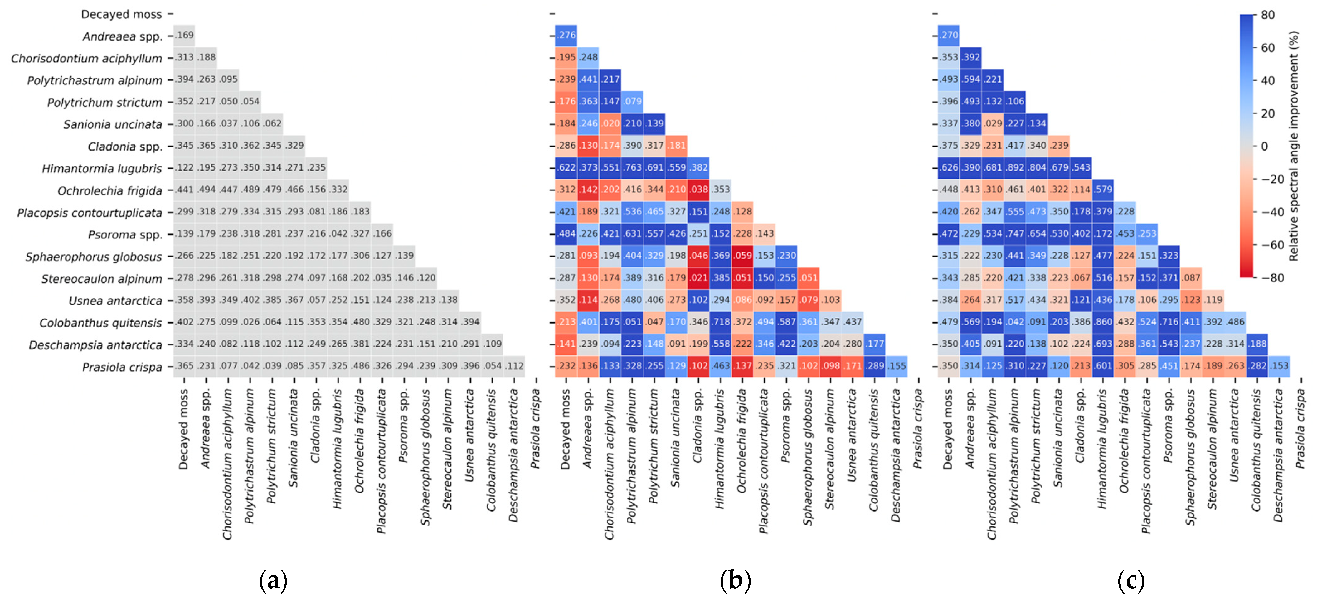
First, whereas only visible and NIR wavelengths have been investigated for the Antarctic vegetation in previous research [25], this study explored a full spectral range and revealed the importance of using SWIR wavelengths for accurately identifying various vegetation classes. The VNIR range could generally explain cell structure and leaf pigments better than longer wavelengths; however, vegetation in cold regions may have relatively weaker spectral signals corresponding to this information and may present stronger water- or biochemical-related information in the SWIR region, compared with vegetation in temperate latitudes. This was tested using individual spectra and simulated image data discussed in Section 3. Particularly, the identification of Deschampsia and Prasiola, which has previously been reported as a challenge when using data from across the VNIR range [25], was improved at 1000–2500 nm.

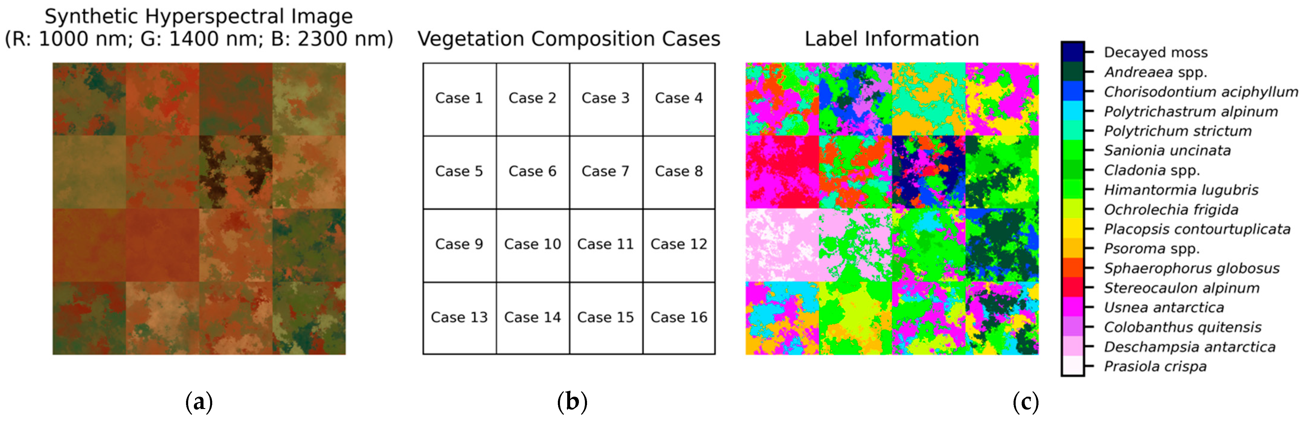
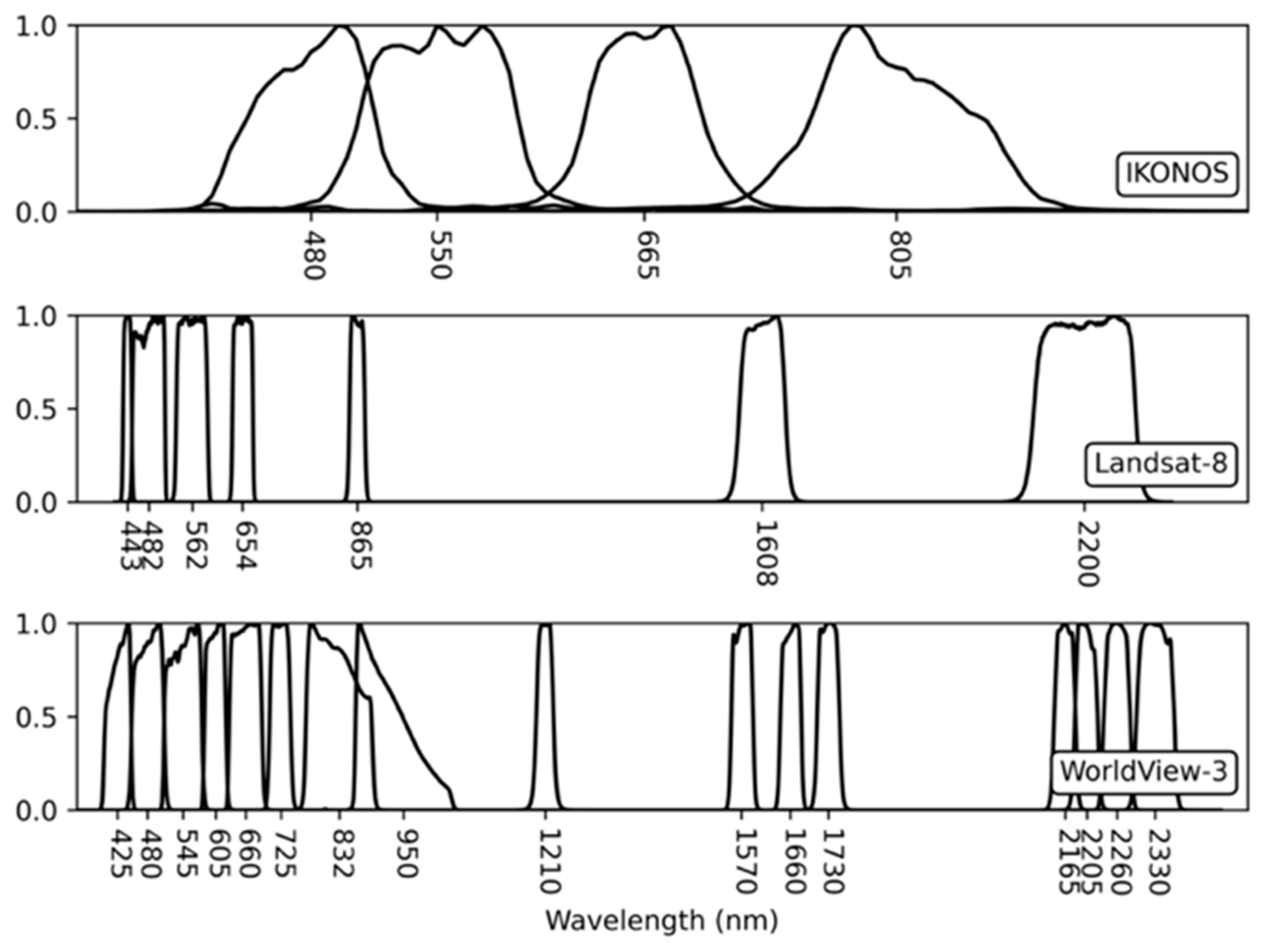
With respect to the second question: the synthetic images in Section 3.3 were generated using library spectra to model popular remote sensing images, including multi- and hyperspectral sensors, owing to the unavailability of real image data for the study area. SAM-based classification and linear unmixing methods were applied to the generated images to investigate which sensor was optimal for analyzing vegetation distributions in practical applications. These experiments represented ideal scenarios since simulated images of known library spectra, using assumed linear mixture models and the ground truth, were used. With true remote sensing imagery, the resulting accuracy will be lower, as it will be difficult to associate the library spectra with the images owing to different data acquisition conditions. However, under the same experimental conditions, hyperspectral data significantly outperformed multispectral sensor data in identifying and quantifying Antarctic vegetation. In particular, these results also indicate that spectral information from the SWIR wavelengths was more effective than that from the VNIR. However, it is worth noting that multispectral sensors showed reasonable classification performance for several dominant species. Particularly, multispectral sensors with more SWIR range bands showed better results than those with fewer bands. Therefore, considering the difficulty in acquiring high-quality hyperspectral data, the purpose of the application, and the vegetation compositions of the study area, the selection of proper remote sensing data would be important.

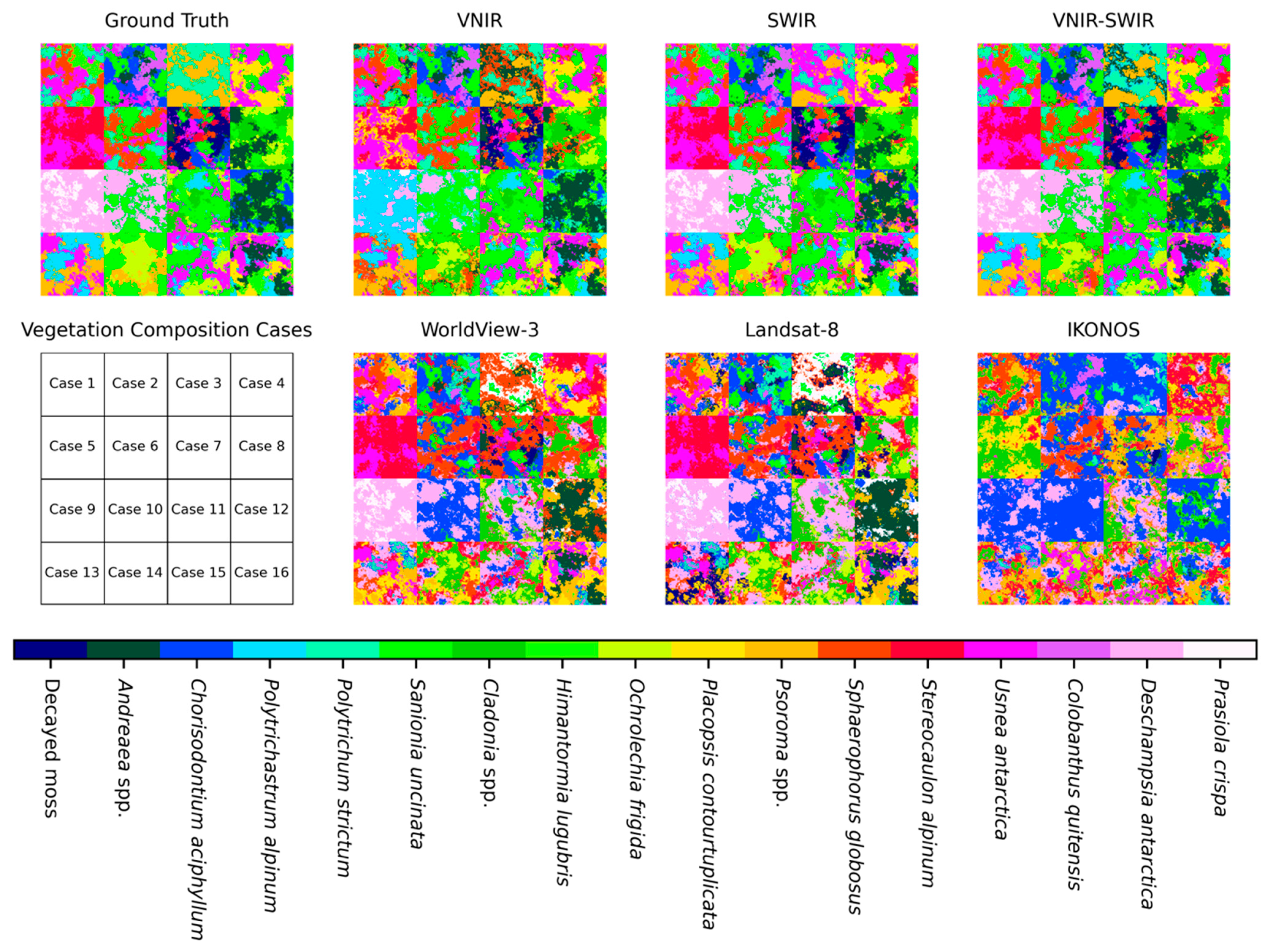
Although we demonstrated the potential performance of several sensors to analyze vegetation species according to their spectral resolutions, it is difficult to conclude which species are clearly separated by which sensor or wavelength region. For example, in Case 12, consisting of Andreaea, Chorisodontium and Himantormia, as shown in Figure 8, the VNIR region images showed better classification results than the SWIR and VNIR-SWIR region images. Some Andreaea and Himantormia pixels in the SWIR and VNIR-SWIR region images were misclassified to Usnea and Psoroma, respectively. However, the Andreaea species in Cases 2, 7, and 16 were successfully identified in both the VNIR and SWIR range data, with even WorldView-3 and Landsat-8 classifying them relatively well, compared with the other species. Himantormia in Cases 1 and 16 were also correctly classified using the VNIR and SWIR datasets. This should indicate that while the spectral resolution of the sensor is crucial, types of species that consist of image pixels are also important for determining the sensor’s classification and unmixing performance.

Conventional surveys assessing vegetation cover over quadrants in the Barton Peninsula have been conducted for several years across sparse locations. However, these surveys are costly, and their findings do not adequately quantify the overall vegetation cover. Recent advances in sensor technologies have facilitated the development of miniaturized hyperspectral sensors for drones. In future work, the spectral library created here, and hyperspectral UAV data should be incorporated to generate detailed vegetation maps of the entire Barton Peninsula, as an alternative to conducting physically intensive field surveys. Satellite remote sensing data, including a new hyperspectral sensor PRISMA (PRecursore IperSpettrale della Missione Applicativa) [54] or high-resolution multispectral data, should also be investigated using the spectral library, based on research goals and sensor performance. In addition, intraspecies spectral variations exist according to color, shape, and environmental conditions. As the spectral library was created with multiple measurements for each species and was temporally distanced from rain or snow events, the spectra used should be considered the most representative signals of the species. However, developing a more detailed library that factors in environmental and physiological conditions is a worthwhile alternative to the potentially destructive contact that currently occurs during the characterization of vegetation.

5. Conclusions

The present study developed a spectral library of 16 major vegetation species and decayed moss in the Barton Peninsula of King George Island, Antarctica, and investigated the interspecies separability and analysis performance using simulated remote sensing imagery. We demonstrated that full-range spectral information was the most effective; however, SWIR range information contributed to better discrimination of the representative vegetation species in the study area than VNIR range information. With respect to practical application using the spectral library and remote sensing data, hyperspectral data are ideal for analyzing vegetation species qualitatively and quantitatively. However, multispectral data with more SWIR range bands showed good performance for several dominant species.

References

1. Grimm, N.B.; Chapin, F.S., III; Bierwagen, B.; Gonzalez, P.; Groffman, P.M.; Luo, Y.; Melton, F.; Nadelhoffer, K.; Pairis, A.; Raymond, P.A. The impacts of climate change on ecosystem structure and function. Front. Ecol. Environ. 2013, 11, 474–482. [Google Scholar] [CrossRef] [Green Version]
2. Longton, R.E. Biology of Polar Bryophytes and Lichens; CUP Archive: Cambridge, UK, 1988. [Google Scholar]
3. Smith, R.L. Signy Island as a Paradigm of Biological and Environmental Change in Antarctic Terrestrial Ecosystems. In Antarctic Ecosystems: Ecological Change and Conservation. SCAR Symposium on Antarctic Biology; Kerry, K.R., Hempel, G., Eds.; Springer: Berlin, Germany, 1990; pp. 32–50. [Google Scholar]
4. Kennedy, A.D. Antarctic terrestrial ecosystem response to global environmental change. Ann. Rev. Ecol. Syst. 1995, 26, 683–704. [Google Scholar] [CrossRef]
5. Convey, P. Terrestrial biodiversity in Antarctica–Recent advances and future challenges. Polar Sci. 2010, 4, 135–147. [Google Scholar] [CrossRef]
6. Turner, J.; Barrand, N.E.; Bracegirdle, T.J.; Convey, P.; Hodgson, D.A.; Jarvis, M.; Jenkins, A.; Marshall, G.; Meredith, M.P.; Roscoe, H.; et al. Antarctic climate change and the environment: An update. Polar Rec. 2014, 50, 237–259. [Google Scholar] [CrossRef] [Green Version]
7. Domack, E.; Leventer, A.; Burnett, A.; Bindschadler, R.; Convey, P.; Kirby, M. Antarctic Peninsula Climate Variability: Historical and Paleoenvironmental Perspectives. In Antarctic Research Series; Domack, E., Leventer, A., Burnett, A., Bindschadler, R., Convey, P., Kirby, M., Eds.; American Geophysical Union: Washington, DC, USA, 2003. [Google Scholar]
8. Kim, J.H.; Ahn, I.-Y.; Lee, K.S.; Chung, H.; Choi, H.-G. Vegetation of Barton Peninsula in the neighbourhood of King Sejong Station (King George Island, maritime Antarctic). Polar Biol. 2007, 30, 903–916. [Google Scholar] [CrossRef]
9. Kim, J.H.; Ahn, I.-Y.; Hong, S.G.; Andreev, M.; Lim, K.-M.; Oh, M.J.; Koh, Y.J.; Hur, J.-S. Lichen flora around the Korean Antarctic Scientific Station, King George Island, Antarctic. J. Microbiol. 2006, 44, 480–491. [Google Scholar]
10. Rodriguez, J.M.; Passo, A.; Chiapella, J.O. Lichen Species Assemblage gradient in South Shetlands Islands, Antarctica: Relationship to deglaciation and microsite conditions. Polar Biol. 2018, 41, 2523–2531. [Google Scholar] [CrossRef]
11. Barcikowski, A.; Gurtowska, J. Studies on the biomass of selected species of Antarctic mosses on King George Island, South Shetland Islands, Antarctica. Pol. Polar Res. 1999, 20, 283–290. [Google Scholar]
12. Ferrari, F.R.; Schaefer, C.E.; Pereira, A.B.; Thomazini, A.; Schmitz, D.; Francelino, M.R. Coupled soil-vegetation changes along a topographic gradient on King George Island, maritime Antarctica. Catena 2021, 198, 105038. [Google Scholar] [CrossRef]
13. Pereira, A.B.; Spielmann, A.A.; Martins, M.F.N.; Francelino, M.R. Plant communities from ice-free areas of Keller peninsula, King George Island, Antarctica. Oecologia Bras. 2007, 11, 14–22. [Google Scholar] [CrossRef]
14. Olech, M.; Słaby, A. Changes in the lichen biota of the Lions Rump area, King George Island, Antarctica, over the last 20 years. Polar Biol. 2016, 39, 1499–1503. [Google Scholar] [CrossRef] [Green Version]
15. Torres-Mellado, G.A.; Jaña, R.; Casanova-Katny, M.A. Antarctic hairgrass expansion in the South Shetland archipelago and Antarctic Peninsula revisited. Polar Biol. 2011, 34, 1679–1688. [Google Scholar] [CrossRef]
16. Putzke, J.; Athanásio, C.G.; De Albuquerque, M.P.; Victoria, F.C.; Pereira, A.B. Comparative study of moss diversity in South Shetland Islands and in the Antarctic Peninsula. Rev. Chil. Hist. Nat. 2015, 88, 822. [Google Scholar] [CrossRef] [Green Version]
17. Théau, J.; Peddle, D.R.; Duguay, C.R. Mapping lichen in a caribou habitat of Northern Quebec, Canada, using an enhancement_classification method and spectral mixture analysis. Remote Sens. Environ. 2005, 94, 232–243. [Google Scholar] [CrossRef]
18. Fretwell, P.T.; Convey, P.; Fleming, A.H.; Peat, H.; Hughes, K.A. Detecting and mapping vegetation distribution on the Antarctic Peninsula from remote sensing data. Polar Biol. 2011, 34, 273–281. [Google Scholar] [CrossRef]
19. Robin, M.; Chapuis, J.-L.; Lebouvier, M. Remote sensing of vegetation cover change in islands of the Kerguelen archipelago. Polar Biol. 2011, 34, 1689–1700. [Google Scholar] [CrossRef]
20. Shin, J.-I.; Kim, H.-C.; Kim, S.-I.; Hong, S.G. Vegetation abundance on the Barton Peninsula, Antarctica: Estimation from high-resolution satellite images. Polar Biol. 2014, 37, 1579–1588. [Google Scholar] [CrossRef]
21. Liu, N.; Treitz, P. Modelling high arctic percent vegetation cover using field digital images and high resolution satellite data. Int. J. Appl. Earth Obs. Geoinf. 2016, 52, 445–456. [Google Scholar] [CrossRef]
22. Sun, X.; Wu, W.; Li, X.; Xu, X.; Li, J. Vegetation abundance and health mapping over Southwestern Antarctica based on worldview-2 data and a modified spectral mixture analysis. Remote Sens. 2021, 13, 166. [Google Scholar] [CrossRef]
23. Clark, R.N. Spectroscopy of rocks and minerals, and principles of spectroscopy. Man. Remote Sens. 1999, 3, 2-2. [Google Scholar]
24. Goswami, S.; Matharasi, K. Development of a web-based vegetation spectral library (Vsl) for remote sensing research and applications. PeerJ PrePrints 2015, 3, e915v1. [Google Scholar]
25. Calviño-Cancela, M.; Martín-Herrero, J. Spectral discrimination of vegetation classes in ice-free areas of Antarctica. Remote Sens. 2016, 8, 856. [Google Scholar] [CrossRef] [Green Version]
26. Jeong, G.; Yoon, H. The Origin of Clay minerals in soils of King George Island, South Shetland Islands, West Antarctica, and its implications for the clay-mineral compositions of marine sediments. J. Sediment. Res. 2001, 71, 833–842. [Google Scholar] [CrossRef]
27. Lee, Y.I.; Lim, H.S.; Yoon, H.I. Geochemistry of soils of King George Island, South Shetland Islands, West Antarctica: Implications for pedogenesis in cold polar regions. Geochim. Cosmochim. Acta 2004, 68, 4319–4333. [Google Scholar] [CrossRef]
28. Cho, H.K.; Kim, J.; Jung, Y.; Lee, Y.G.; Lee, B.Y. Recent changes in downward longwave radiation at King Sejong station, Antarctica. J. Clim. 2008, 21, 5764–5776. [Google Scholar] [CrossRef]
29. Nicodemus, F.E.; Richmond, J.C.; Hsia, J.J.; Ginsberg, I.; Limperis, T. Geometrical considerations and nomenclature for reflectance. NBS Mono. 1992, 160, 4. [Google Scholar]
30. Painter, T.H.; Molotch, N.P.; Cassidy, M.; Flanner, M.; Steffen, K. Contact spectroscopy for determination of stratigraphy of snow optical grain size. J. Glaciol. 2007, 53, 121–127. [Google Scholar] [CrossRef] [Green Version]
31. Hueni, A.; Bialek, A. Cause, effect, and correction of field spectroradiometer interchannel radiometric steps. IEEE J. Sel. Top. Appl. Earth Obs. Remote Sens. 2017, 10, 1542–1551. [Google Scholar] [CrossRef]
32. Mac Arthur, A.; MacLellan, C.J.; Malthus, T. The fields of view and directional response functions of two field spectroradiometers. IEEE Trans. Geosci. Remote Sens. 2012, 50, 3892–3907. [Google Scholar] [CrossRef]
33. Chang, C.-I. Spectral information divergence for hyperspectral image analysis. In Proceedings of the IEEE 1999 International Geoscience and Remote Sensing Symposium, IGARSS’99 (Cat. No.99CH36293), Hamburg, Germany, 28 June–2 July 1999; Institute of Electrical and Electronics Engineers (IEEE): Hamburg, Germany, 2003; Volume 1, pp. 509–511. [Google Scholar]
34. der Meer, F.V. The effectiveness of spectral similarity measures for the analysis of hyperspectral imagery. Int. J. Appl. Earth Obs. Geoinf. 2006, 8, 3–17. [Google Scholar] [CrossRef]
35. Van Der Meero, F.; Bakker, W. Cross correlogram spectral matching: Application to surface mineralogical mapping by using AVIRIS data from Cuprite, Nevada. Remote Sens. Environ. 1997, 61, 371–382. [Google Scholar] [CrossRef]
36. Yuhas, R.H.; Goetz, A.F.; Boardman, J.W. Discrimination among semi-arid landscape endmembers using the Spectral Angle Mapper (Sam). Algorithm 1992, 1, 147–149. [Google Scholar]
37. Shivakumar, B.R.; Rajashekararadhya, S.V. Performance évaluation of spectral angle mapper and spectral correlation mapper classifiers over multiple remote sensor data. In Proceedings of the 2017 Second International Conference on Electrical, Computer and Communication Technologies (ICECCT), Coimbatore, India, 22–24 February 2017; pp. 1–6. [Google Scholar] [CrossRef]
38. Kim, S.C. Vegetation Distribution Pattern on Barton Peninsula of King George Island, Antarctica. Ph.D. Thesis, Gangneung-Wonju National University, Wonju, Korea, 2016. [Google Scholar]
39. Barry, P.; Mendenhall, J.; Jarecke, P.; Folkman, M.; Pearlman, J.; Markham, B. EO-1 Hyperion hyperspectral aggregation and comparison with EO-1 Advanced Land Imager and Landsat 7 ETM+. In Proceedings of the IEEE International Geoscience and Remote Sensing Symposium, Toronto, ON, Canada, 24–28 June 2002; Volume 3, pp. 1648–1651. [Google Scholar] [CrossRef]
40. Kruse, F.; Lefkoff, A.; Boardman, J.; Heidebrecht, K.; Shapiro, A.; Barloon, P.; Goetz, A. The spectral image processing system (SIPS)—Interactive visualization and analysis of imaging spectrometer data. Remote Sens. Environ. 1993, 44, 145–163. [Google Scholar] [CrossRef]
41. Keshava, N.; Mustard, J.F. Spectral unmixing. IEEE Signal Process. Mag. 2002, 19, 44–57. [Google Scholar] [CrossRef]
42. Knipling, E.B. Physical and physiological basis for the reflectance of visible and near-infrared radiation from vegetation. Remote Sens. Environ. 1970, 1, 155–159. [Google Scholar] [CrossRef]
43. Shengyan, D.; Jidong, G.; Lexiang, Q. Assessment of biochemical concentrations of vegetation using remote sensing technology. J. Geogr. Sci. 2002, 12, 321–330. [Google Scholar] [CrossRef]
44. Deepak, M.; Keski-Saari, S.; Fauch, L.; Granlund, L.; Oksanen, E.; Keinänen, M. Leaf canopy layers affect spectral reflectance in silver birch. Remote Sens. 2019, 11, 2884. [Google Scholar] [CrossRef] [Green Version]
45. Granlund, L.; Keski-Saari, S.; Kumpula, T.; Oksanen, E.; Keinänen, M. Imaging lichen water content with visible to mid-wave infrared (400–5500 nm) spectroscopy. Remote Sens. Environ. 2018, 216, 301–310. [Google Scholar] [CrossRef]
46. Rees, W.; Tutubalina, O.; Golubeva, E. Reflectance spectra of subarctic lichens between 400 and 2400 nm. Remote Sens. Environ. 2004, 90, 281–292. [Google Scholar] [CrossRef]
47. Daughtry, C.S. Discriminating crop residues from soil by shortwave infrared reflectance. Agron. J. 2001, 93, 125–131. [Google Scholar] [CrossRef]
48. Bechtel, R.; Rivard, B.; Sánchez-Azofeifa, A. Spectral properties of foliose and crustose lichens based on laboratory experiments. Remote Sens. Environ. 2002, 82, 389–396. [Google Scholar] [CrossRef]
49. Curran, P.J. Remote sensing of foliar chemistry. Remote Sens. Environ. 1989, 30, 271–278. [Google Scholar] [CrossRef]
50. Slaton, M.R.; Hunt, E.R.; Smith, W.K. Estimating near-infrared leaf reflectance from leaf structural characteristics. Am. J. Bot. 2001, 88, 278–284. [Google Scholar] [CrossRef] [PubMed]
51. Kuska, M.T.; Behmann, J.; Mahlein, A.-K. Potential of hyperspectral imaging to detect and identify the impact of chemical warfare compounds on plant tissue. Pure Appl. Chem. 2018, 90, 1615–1624. [Google Scholar] [CrossRef]
52. Fowbert, J.A. An experimental study of growth in relation to morphology and shoot water content in maritime Antarctic mosses. New Phytol. 1996, 133, 363–373. [Google Scholar] [CrossRef] [PubMed]
53. Proctor, M.C.; Nagy, Z.; Csintalan, Z.; Takács, Z. Water-content components in bryophytes: Analysis of pressure-volume relationships. J. Exp. Bot. 1998, 49, 1845–1854. [Google Scholar] [CrossRef]
54. Giacomo, C.; Ettore, L.; Rino, L.; Rosa, L.; Rocchina, G.; Girolamo, D.M.; Patrizia, S. The hyperspectral prisma mission in operations. In Proceedings of the IGARSS 2020—2020 IEEE International Geoscience and Remote Sensing Symposium, Waikoloa, HI, USA, 26 September–2 October 2020; pp. 3282–3285. [Google Scholar]
Figure 1. Location and geographic map of Barton Peninsula in King George Island, the largest of the South Shetland Islands.
Remotesensing 13 02470 g001
Figure 2. Example of mixed vegetation species for Case 7 (Andreaea, Chorisodontium, Sanionia, Sphaerophorus, Stereocaulon, Usnea, decayed moss).
Remotesensing 13 02470 g002
Figure 3. Simulated fractional abundance images of 16 vegetation species and decayed moss generated by the Spheric Gaussian Fields method.
Remotesensing 13 02470 g003
Figure 4. (a) Generated and combined synthetic hyperspectral images for each (b) vegetation compositional cases as defined in Table 2. (c) Class labels as defined by the most dominant fractional abundances.
Remotesensing 13 02470 g004
Figure 5. Spectral response functions of popular multispectral remote sensing sensors (IKONOS, Landsat-8, WorldView-3) used to aggregate hyperspectral data into multispectral images. Center wavelength for each band is denoted on the x-axes. The y-axes show relative spectral response.
Remotesensing 13 02470 g005
Figure 6. Spectral reflectance curves of 16 representative vegetation species and decayed moss in the Barton Peninsula, for: (a) mosses; (b) lichens; (c) vascular plants and alga group. x-axes show wavelength (nm), and y-axes show reflectance.
Remotesensing 13 02470 g006aRemotesensing 13 02470 g006b
Figure 7. Spectral angle comparisons of 16 vegetation species and decayed moss for the (a) VNIR, 400–1000 nm; (b) SWIR, 1000–2500 nm; and (c) VNIR-SWIR 400–2500 nm ranges. Relative spectral angle improvements with respect to the 400–1000 nm range are color-coded (positive improvements, blue; negative improvements, red).
Remotesensing 13 02470 g007
Figure 8. Classified vegetation species maps across different wavelengths and sensors, generated by spectral angle mappers according to the developed spectral library.
Remotesensing 13 02470 g008