Azimuth Resolution Improvement and Target Parameters Inversion for Distributed Shipborne High Frequency Hybrid Sky-Surface Wave Radar

Abstract

In this paper, the aperture synthesis processing techniques for the distributed shipborne high frequency hybrid sky-surface wave radar (HFHSSWR) are proposed to improve the azimuth resolution and obtain the velocity vector and the azimuth estimation of the moving target. First, the system geometry and the signal model of the moving target for the distributed shipborne HFHSSWR are formulated, and then the azimuth resolution improvement principle is derived. Second, based on the developed signal model, we propose an azimuth resolution improvement algorithm, which can obtain the synthetic azimuth bandwidth and an improved resolution using sub-band combination. Finally, a target parameters inversion method is introduced to estimate the target velocity vector and the target azimuth, by solving the equations regarding the target geometry and echo signal parameters numerically. The simulations are performed to verify the proposed algorithms. The results indicate that the distributed synthetic aperture techniques effectively improve the azimuth resolution of this radar, and can obtain the target velocity vector and the high-precision estimation of the target azimuth.

1. Introduction

The shipborne high frequency (HF) hybrid sky-surface wave radar (HFHSSWR) is a new system containing a skywave transmitting path and a surface wave receiving path, in which the receiving station is placed on a shipborne platform [1,2,3]. The shipborne HFHSSWR not only maintains the capacity of long range over the horizon target detection and wide-area coverage of the HF sky-wave radar, but also retains the stability and long integration time of the HF surface wave radar (HFSWR). It also has the advantage of maneuverability of the shipborne HFSWR, which has an advancement in wide-area surveillance of over-the-horizon targets and ocean environment [4,5,6,7,8,9,10,11,12,13,14,15,16,17]. However, the shipborne HFHSSWR suffers from low azimuth resolution and poor estimation accuracy in azimuth, due to the small array aperture limited by the confined space on a shipborne platform. The distributed shipborne HFHSSWR with multiple receiving ships provides a solution to these challenges when ships sail in formation. As a coherent radar system, this radar has the potential to achieve a larger aperture by the multi-platform data fusion.

For achieving a large aperture by signal analysis, the synthetic aperture radar (SAR), consisting of a sensor mounted on a moving platform, can improve its azimuth resolution by utilizing the Doppler spread of the echo signal, which has been widely used for earth remote sensing [18,19]. The SAR system operating in the HF-band is called HF SAR, which has been placed on spaceborne, airborne and shipborne platforms. The applications of HF SAR systems include planetary surface image generation [20,21], topside ionosphere exploration [22,23], ocean wave spectra measurement [24,25], and ocean surface current extraction [26,27], etc. The azimuth resolution of most SAR systems is independent of range. This requires an increasing synthetic aperture length and integration times necessarily as range increases. However, the upper bound of the synthetic aperture length is commonly not available for the shipborne HF SAR, due to the limited integration time and slow ship speeds. Naturally, the distributed shipborne HF SAR can break through the limitation of the short synthetic aperture length within the limited integration time for a single shipborne HF SAR, by combining observations of multiple platforms with slightly different viewing angles.

The azimuth resolution of a SAR system is determined by the Doppler (azimuth) bandwidth of the echo signal [19]. A high azimuth resolution can be achieved by a large azimuth bandwidth. Therefore, a distributed SAR can obtain an equivalent large aperture by increasing the azimuth bandwidth using the spectral synthesis technique. There have been similar studies to increase the resolution through spectral synthesis for spaceborne and airborne distributed SAR systems operating in the microwave band. Among these works, the images acquired with slightly different viewing angles are coherently combined to increase the range bandwidth based on the spectral shift principle, and thus, the range resolution of a distributed SAR is improved [28,29,30,31,32,33,34,35]. This paper draws on the core idea of range resolution improvement algorithms of spaceborne and airborne SAR images and focuses on improving the azimuth resolution of the distributed shipborne HFHSSWR system by spectral synthesis. Meanwhile, we also desire to obtain the target velocity vector and the high-precision estimation of the target azimuth, due to the interest in the problem of target monitoring. Fortunately, the azimuth resolution improvement will help to increase the azimuth estimation accuracy [36]. The distributed radar system can also obtain the target velocity vector rather than just radial velocity utilizing the multi-angle observations.

In this paper, we propose the aperture synthesis processing techniques for the distributed shipborne HFHSSWR system, to improve the azimuth resolution and obtain the velocity vector and the azimuth estimation of the moving target. For simplicity, this work only analyzes the azimuth resolution improvement and the target parameters inversion in the case of a quiet ionosphere, such as quiet mid-latitude paths [37], and shipborne platforms with uniform linear motion. First, we build a baseband echo signal model of the moving target for this system and derive the basic azimuth resolution improvement principle. Second, based on the developed model, an azimuth resolution improvement algorithm of the moving target is presented to achieve a higher azimuth resolution. Then, a target parameters inversion method is proposed to obtain the high-precision estimation of the target azimuth and the estimation of the target velocity vector that is not available for a single shipborne HFHSSWR. Finally, numerical results are provided to verify the proposed algorithms. The comparison simulation shows that the azimuth compression result of the distributed shipborne HFHSSWR system has a narrower main lobe width and a higher peak pulse power than those of a single shipborne HFHSSWR. Additionally, compared to the single radar, the distributed radar system has a better performance in the estimation of target velocity vector and azimuth parameters.

The structure of this paper is as follows. In Section 2, the system geometry and the signal model of the distributed shipborne HFHSSWR system are established, and the principle of improving azimuth resolution is derived. Then, based on the signal model, an azimuth resolution improvement algorithm and a target parameters inversion method are proposed in Section 3 and Section 4, respectively. Section 5 provides the simulation of the proposed aperture synthesis processing techniques for the distributed radar system. The discussion of these results and algorithms is given in Section 6. Finally, Section 7 concludes the paper.

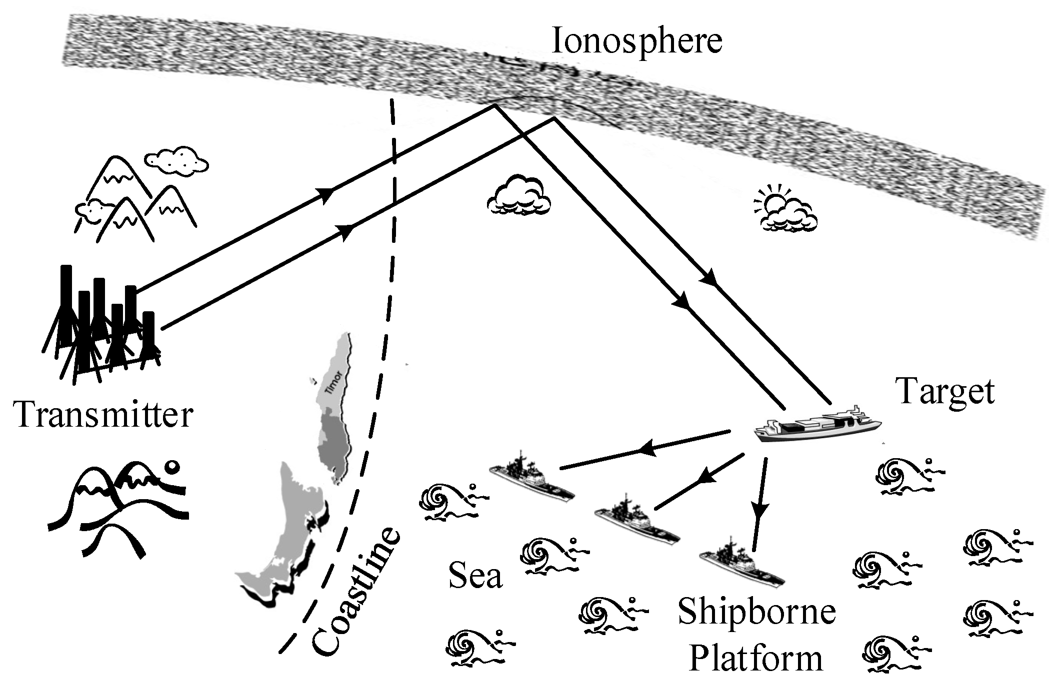
2. Azimuth Resolution Improvement of the Moving Target via Spectral Synthesis

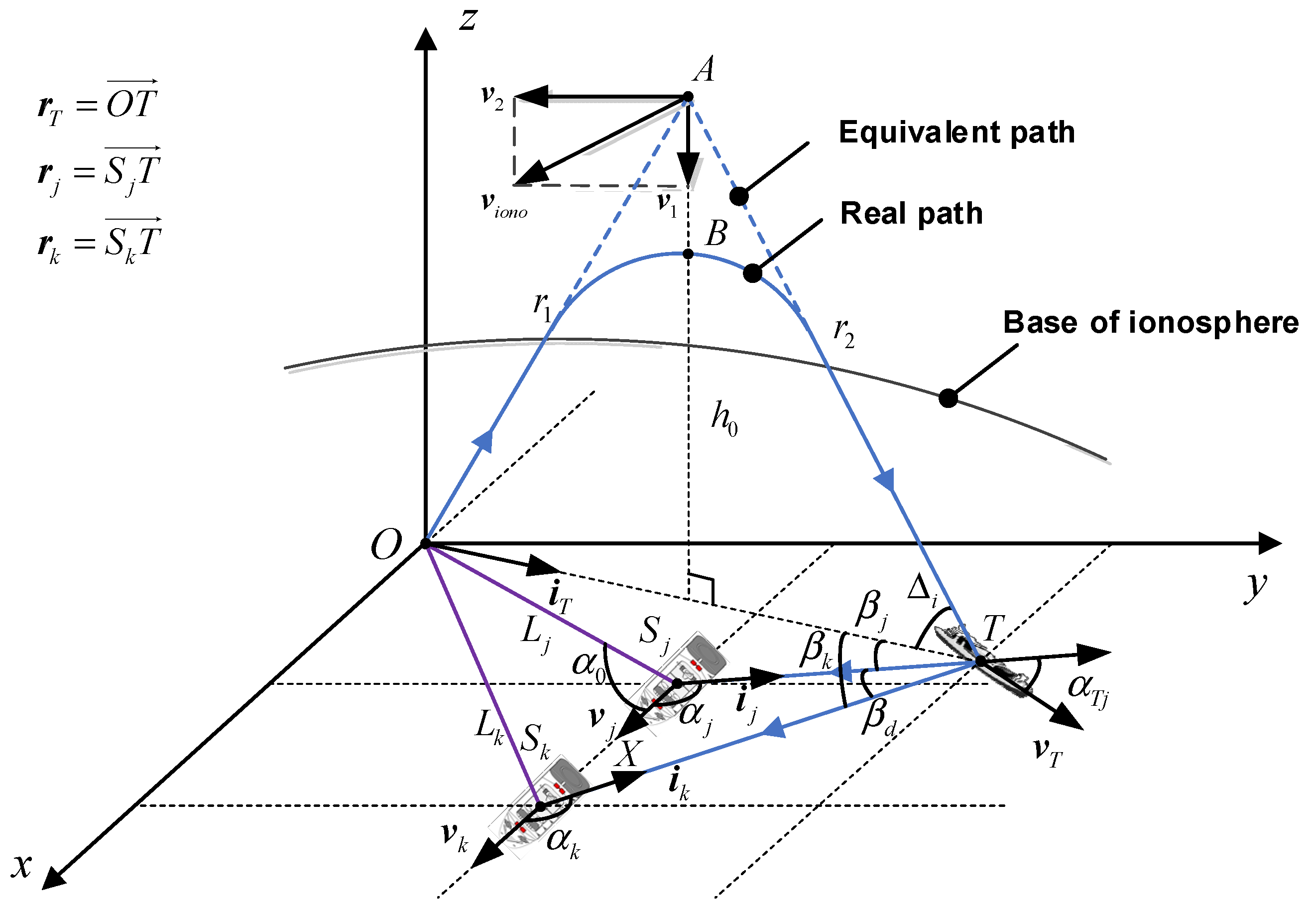
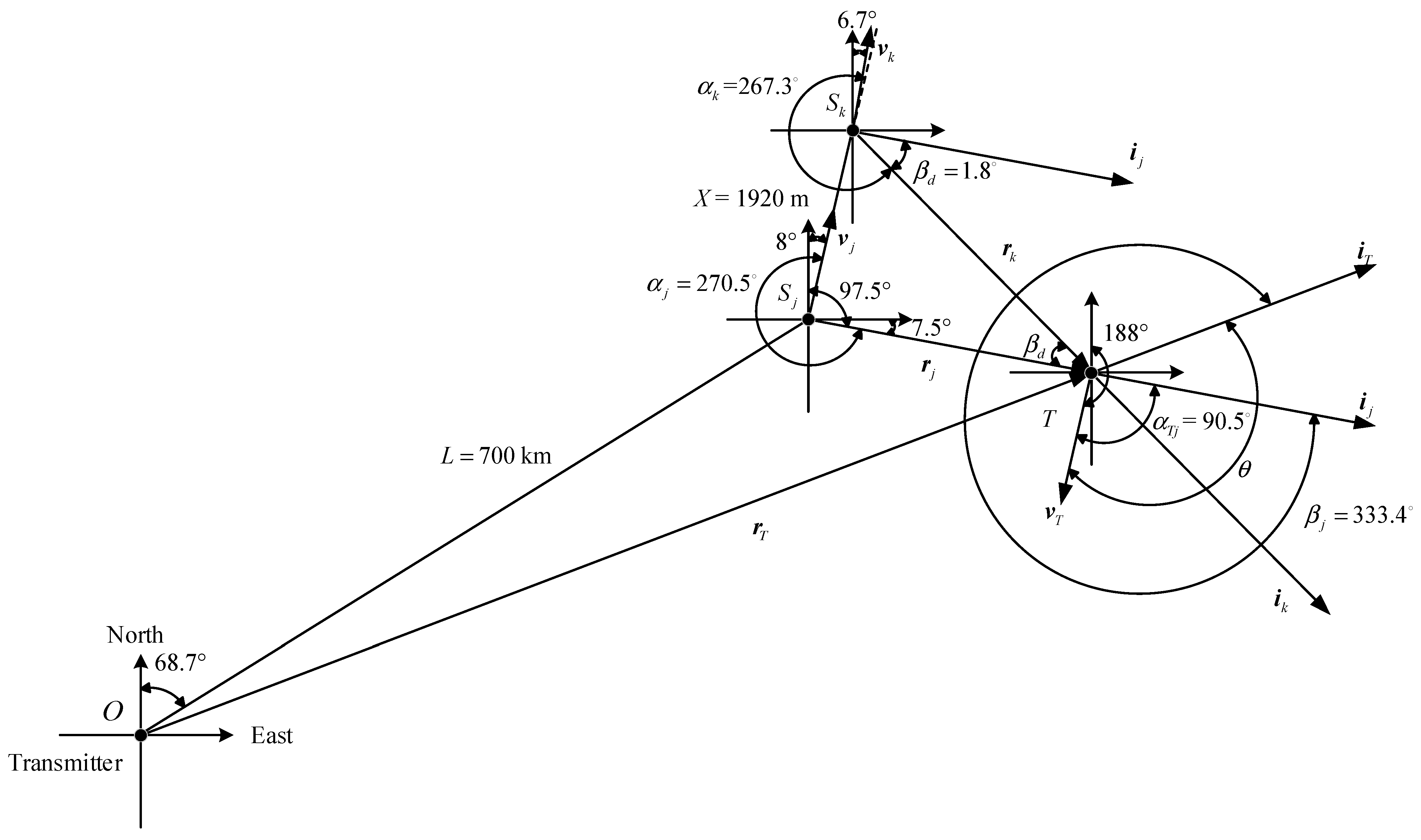
The distributed shipborne HFHSSWR system consists of one transmitter located inland and M receiving ships, as shown in Figure 1. The transmitter transmits a chirp signal, which is reflected from the ionosphere to illuminate sea surface targets. The scattered surface wave signal is received by the receiving array through ground-wave propagation across the ocean. The receiving antenna array aperture along the side of each receiving ship is D. Assuming that the synthetic aperture of a single ship is L, the originality of the concept of the distributed synthetic aperture for the distributed shipborne HFHSSWR is that the integration time adapted to the total synthetic aperture length $M\cdot L$ is reduced by a factor of M. Figure 2 shows a conceptual diagram of the distributed synthetic aperture.

In this section, we first build a signal model of the moving target based on the distributed shipborne HFHSSWR configuration. Then, the principle of the azimuth resolution improvement is discussed according to this model.

2.1. Signal Model

In the three-dimensional Cartesian coordinate system with the transmitter as the coordinate origin O, the system geometry of the distributed shipborne HFHSSWR reconnoitering a ship target T is shown in Figure 3, where the curvature of the earth is ignored. Only two shipborne platforms $S_j$ and $S_k$ are given to simplify the analysis. The two ships sail along the same direction at similar speeds. The transmitter, shipborne platforms and the target lie in the x-y plane, i.e., ground plane. The x axis is tangent to the Earth surface and parallel to the velocity vector of the platform $S_j$. The y axis and z axis are perpendicular to the x axis and the ground plane, respectively. The geometric parameters in Figure 3 are defined as follows.

• $r_1$: half the length of the sky-wave path, which is equal to $r_2$;
• ${\mathit{r}}_T$: position vector from O to T, where $r_T$ is the magnitude of ${\mathit{r}}_T$;
• $h_0$: virtual reflection height;
• ${\mathit{v}}_T$: velocity vector of the target T (with magnitude $v_T$);
• ${\mathit{v}}_j$: velocity vector of the shipborne platform $S_j$ (with magnitude $v_j$);
• ${\mathit{v}}_{iono}$: velocity vector of the ionospheric reflector, which can be decomposed into the vertical component ${\mathit{v}}_1$ and the horizontal component ${\mathit{v}}_2$.
• ${\mathit{r}}_j$: position vector from $S_j$ to T, where $r_j$ is the magnitude of ${\mathit{r}}_j$, ${\mathit{i}}_j$ is the unit vector in the direction of ${\mathit{r}}_j$;
• ${\beta }_j$: clockwise rotation angle from ${\mathit{r}}_j$ to ${\mathit{r}}_T$, i.e., bistatic angle;
• ${\beta }_d$: clockwise rotation angle from ${\mathit{r}}_j$ to ${\mathit{r}}_k$;
• $L_j$: ground distance between the transmitter O and the receiver $S_j$, i.e., baseline length;
• ${\alpha }_0$: clockwise rotation angle from ${\mathit{v}}_j$ to the position vector from $S_j$ to O;
• ${\alpha }_j$: clockwise rotation angle from ${\mathit{r}}_j$ to ${\mathit{v}}_j$,which denotes the target direction;
• ${\alpha }_{Tj}$: clockwise rotation angle from ${\mathit{r}}_j$ to ${\mathit{v}}_T$;
• ${\Delta }_i$: grazing angle.

The definition and the symbolic representation of the geometric parameters corresponding to $S_k$ are the same as those of $S_j$, except that the subscript is k. The distance between $S_k$ and $S_j$ is X.

The most important parameter in SAR processing is the slant range from the radar to targets [19]. Accordingly, the group-range of an echo from a surface-target in the distributed shipborne HFHSSWR system is the key parameter. The group-range varying with the azimuth time (slow time) $\eta$ is defined by the range equation. If we assume a horizontally stratified ionosphere and ignore tilts and gradients (geometry as shown in Figure 3), then by applying the Breit-Tuve theorem [37,38,39,40], the real curved ray path $P^{\prime }$ for the radio wave to travel between points O and T via point B in the ionosphere is identical to that which would be taken along the virtual rectilinear path OAT. Therefore, the ionospheric reflection is assumed to be a specular reflection. For the shipborne platform $S_j$, the range equation of the target T is given by

$$d_j\left(\eta \right)=P^{\prime }\left(\eta \right)+r_{j\eta }=\left(r_{1\eta }+r_{2\eta }\right)+r_{j\eta }=2\cdot \sqrt{{\left(r_{T\eta }/2\right)}^2+h_{\eta }{}^2}+r_{j\eta },$$

(1)

where $r_{T\eta }=\left|{\mathit{r}}_T+{\mathit{v}}_T\cdot \eta \right|$, $r_{j\eta }=\left|{\mathit{r}}_j+\left({\mathit{v}}_T-{\mathit{v}}_j\right)\cdot \eta \right|$ and $h_{\eta }$ is the virtual height at time $\eta$. Let the ionosphere move with a uniform velocity $v_1$ in the vertical direction (the upward direction is taken as positive), then

$$h_{\eta }=h_0+v_1\cdot \eta .$$

(2)

The second Taylor approximation of $r_{T\eta }$ at $\eta =0$ is

$$r_{T\eta }\approx r_T+v_T\cdot \cos \theta \cdot \eta +\frac{v_T{}^2{\sin }^2\theta }{2r_T}\cdot {\eta }^2,$$

(3)

where $\cos \theta =〈{\mathit{r}}_T,{\mathit{v}}_T〉/\left(r_T\cdot v_T\right)=\cos \left({\alpha }_{Tj}-{\beta }_j\right)$, and $〈\mathit{a},\mathit{b}〉$ denotes the inner product of vectors $\mathit{a}$ and $\mathit{b}$. Similarly, the distance between $S_j$ and T is given by

$$r_{j\eta }\approx r_j+\left|{\mathit{v}}_T-{\mathit{v}}_j\right|\cdot \cos \alpha \cdot \eta +\frac{{\left|{\mathit{v}}_T-{\mathit{v}}_j\right|}^2{\sin }^2\alpha }{2r_j}\cdot {\eta }^2,$$

(4)

where $\cos \alpha =〈{\mathit{r}}_j,{\mathit{v}}_T-{\mathit{v}}_j〉/\left(r_j\cdot \left|{\mathit{v}}_T-{\mathit{v}}_j\right|\right)=\left(v_T\cdot \cos {\alpha }_{Tj}-v_j\cdot \cos {\alpha }_j\right)/\left|{\mathit{v}}_T-{\mathit{v}}_j\right|$.

From Equations (1) to (4), the range equation can be expressed as

$$d_j\left(\eta \right)=d_{j0}+\Delta d_j\left(\eta \right),$$

(5)

where $d_{j0}$ and $\Delta d_j\left(\eta \right)$ can be calculated as follows

$$d_{j0}=2r_1+r_j=2\cdot \sqrt{{\left(r_T/2\right)}^2+h_0{}^2}+r_j,$$

(6)

$$\Delta d_j\left(\eta \right)=-\lambda f_{acj}\cdot \eta -\frac{\lambda }{2}{K}_{aj}{\eta }^2,$$

(7)

$$f_{acj}=-\frac{1}{\lambda }\left[\cos {\Delta }_i\cdot v_T\cdot \cos \left({\alpha }_{Tj}-{\beta }_j\right)+\left(v_T\cdot \cos {\alpha }_{Tj}-v_j\cdot \cos {\alpha }_j\right)+2\sin {\Delta }_i\cdot v_1\right],$$

(8)

$$K_{aj}=-\frac{1}{\lambda }\left[\begin{array}{l}-\frac{{\left(2\sin {\Delta }_i{v}_1+\cos {\Delta }_i{v}_T\cos \left({\alpha }_{Tj}-{\beta }_j\right)\right)}^2}{2r_1}+\frac{v_T{}^2+4v_1{}^2}{2r_1}+\\ \frac{v_T{}^2{\sin }^2{\alpha }_{Tj}+v_j{}^2\cdot {\sin }^2{\alpha }_j-2v_T{v}_j\left(\cos \left({\alpha }_{Tj}-{\alpha }_j\right)-\cos {\alpha }_{Tj}\cos {\alpha }_j\right)}{r_j}\end{array}\right].$$

(9)

where $\cos {\Delta }_i=r_T/2r_1$, $\lambda$ is the radar wavelength, and the expressions of $f_{acj}$ and $K_{aj}$ are obtained by the second Taylor approximation of $d_j\left(\eta \right)$ at $\eta =0$.

From Equations (5) and (9), it can be seen that the received signal in the azimuth direction is the chirp signal with linear FM (LFM) characteristics. More specifically, the azimuth frequency (Doppler frequency) of the echo received by the shipborne platform $S_j$ from the target T is

$$f_{aj}=-\frac{1}{\lambda }\cdot \frac{d}{d\eta }\left(d_{j0}+\Delta d_j\left(\eta \right)\right)=f_{acj}+K_{aj}\eta ,$$

(10)

where $f_{acj}$ is the initial Doppler frequency and $K_{aj}$ is the azimuth frequency modulation (FM) rate, which are constants for a given system geometry and a target motion state.

The range equation and the azimuth frequency of the target T for the shipborne platform $S_k$ can be obtained using a similar derivation (see Appendix A).

The above derivation provides the geometric model of the target for the distributed shipborne HFHSSWR. Next, the received signal model of the target for this radar can be derived based on the geometric model. Consider an LFM pulse signal as the transmitting signal, as given by

$$s_{pul}\left(\tau \right)={\omega }_r\left(\tau \right)\cos \left(2\pi f_0\tau +\pi K_r{\tau }^2\right),$$

(11)

where ${\omega }_r\left(\tau \right)=\mathrm{rect}\left(\frac{\tau }{T_r}\right)$, $\mathrm{rect}[u]=\left\{\begin{array}{cc}1,& \left|u\right|\le 1/2\\ 0,& \left|u\right|>1/2\end{array}\right.$, $T_r$ is the pulse duration, $\tau$ is the range time, i.e., fast time, $K_r$ is the FM rate of the range pulse and $f_0$ is the center frequency.

Then, the demodulated baseband signal can be given by [19]

$$\begin{array}{l}{s}_0\left(\tau ,\eta \right)=A_0{\omega }_r\left(\tau -\frac{d\left(\eta \right)}{c}\right)\exp \left\{j\pi K_r{\left(\tau -\frac{d\left(\eta \right)}{c}\right)}^2\right\}\\ \hspace{1em}\hspace{1em}\hspace{1em}\hspace{1em}\times {\omega }_a\left(\eta -{\eta }_c\right)\exp \left\{-j2\pi f_0\frac{d_0}{c}\right\}\exp \left\{j2\pi f_{ac}\cdot \eta +j\pi K_a{\eta }^2\right\}+n\left(\tau ,\eta \right)\end{array}$$

(12)

where $A_0$ is a complex constant, ${\eta }_c$ is the beam center offset time, ${\omega }_r\left(\tau \right)$ is a rectangular function (range envelope), ${\omega }_a\left(\eta \right)$ is a sinc function (azimuth envelope), and $n\left(\tau ,\eta \right)$ is the stationary complex white Gaussian noise with zero-mean and variance ${\sigma }_n^2$.

As mentioned earlier, it should be noted that Equation (12) is obtained in the case of a quiet ionosphere, such as quiet mid-latitude paths [37], and shipborne platforms with uniform linear motion, and it is assumed that the suppression of the sea clutter is completed. However, for the non-ideal cases, such as ionospheric disturbances and the six degree-of-freedom (DOF) motion of shipborne platforms, the model needs to be improved, which is beyond the scope of this paper and can be analyzed separately [41,42,43,44,45,46,47,48,49].

2.2. Improvement of the Azimuth Resolution

In this section, the basic azimuth resolution improvement principle for the distributed shipborne HFHSSWR system is derived. First, we briefly analyze the aperture time required for the shipborne HFHSSWR to obtain the maximum synthetic aperture length, in order to illustrate the great potential of the distributed radar system for improving the azimuth resolution. Then, the inverse relation between the azimuth resolution and the azimuth bandwidth is briefly described. Finally, based on the spectral shift, the azimuth resolution improvement principle for the distributed system radar is introduced.

(1)

The aperture time to obtain the maximum synthetic aperture length.

The lower bound on sidelooking strip-map monostatic SAR azimuth (cross range) resolution is approximately one-half the antenna length D, which requires an aperture time proportional to range. However, the lower bound on shipborne HFHSSWR azimuth resolution is commonly not available due to the limited aperture time and slow ship speeds. As an example, let $D=50\hspace{1em}\mathrm{m}$, $\lambda =30\hspace{1em}\mathrm{m}$, $r_j=100\hspace{1em}\mathrm{km}$, and assume a small squint angle. The obtainable synthetic aperture length is

$$L=\frac{0.886\lambda \cdot r_j}{D}=53.16\hspace{1em}\mathrm{km}.$$

(13)

Assuming that $V_j=15$ m/s and the receiving ship sails in a straight line, the aperture time to obtain this synthetic aperture is up to one hour, which is generally not achievable in a shipborne HFHSSWR system. This means that the total synthetic aperture length of the distributed shipborne HFHSSWR system has much room for improvement, as the distributed radar system requires much less aperture time to obtain the same aperture length than a single shipborne HFHSSWR.

(2)

The inverse relation between the azimuth resolution and the azimuth bandwidth.

According to Equation (10), the signal in the azimuth direction is frequency modulated by the platform motion. Hence, we can obtain a high azimuth resolution by matched filtering as in the range direction. The azimuth resolution ${\rho }_a$ (in time units) is equal to the reciprocal of the azimuth bandwidth $B_a$ [19], which is given by

$${\rho }_a=1/B_a.$$

(14)

where $B_a=T_a\cdot \left|K_a\right|$, and $T_a$ is the aperture time, i.e., coherent integration time (CIT). This indicates that the azimuth resolution can be improved by increasing the azimuth bandwidth.

(3)

The azimuth resolution improvement principle.

Next, we will analyze the Doppler spectral shift between two signals coming from two different platforms, to explore the possibility of increasing the azimuth bandwidth of the distributed shipborne HFHSSWR system by spectral synthesis. From Equations (10) and (A5), we can obtain the azimuth frequency difference

$$\begin{array}{l}\Delta f_a=f_{aj}-f_{ak}=f_{acj}-f_{ack}+\left(K_{aj}-K_{ak}\right)\eta \\ =-\frac{1}{\lambda }\left[v_T\cdot \left(\cos {\alpha }_{Tj}-\cos {\alpha }_{Tk}\right)-v_j\cdot \cos {\alpha }_j+v_k\cdot \cos {\alpha }_k\right]\\ -\frac{1}{\lambda }\left[\begin{array}{l}\frac{v_T{}^2{\sin }^2{\alpha }_{Tj}+v_j{}^2\cdot {\sin }^2{\alpha }_j-2v_T{v}_j\left(\cos \left({\alpha }_{Tj}-{\alpha }_j\right)-\cos {\alpha }_{Tj}\cos {\alpha }_j\right)}{r_j}\\ -\frac{v_T{}^2{\sin }^2{\alpha }_{Tk}+v_k{}^2\cdot {\sin }^2{\alpha }_k-2v_T{v}_k\left(\cos \left({\alpha }_{Tk}-{\alpha }_k\right)-\cos {\alpha }_{Tk}\cos {\alpha }_k\right)}{r_k}\end{array}\right]\eta \\ \approx -\frac{1}{\lambda }\left[\left(v_T\cdot \cos {\alpha }_{Tj}-v_j\cdot \cos {\alpha }_j\right)+\left(v_k\cdot \cos {\alpha }_k-v_T\cdot \cos {\alpha }_{Tk}\right)\right]\end{array}$$

(15)

In Equation (15), the terms containing azimuth time $\eta$ can be ignored for the case of slow ship targets (the speeds of targets and receiving ships are about 10 m/s, $r_j$ and $r_k$ can extend to a few hundred kilometers). Particularly, when $v_j=v_k=v$ and $v_T=0$, Equation (15) can be simplified as

$$\Delta f_a\approx -\frac{1}{\lambda }\left[v\cdot \left(\cos {\alpha }_k-\cos {\alpha }_j\right)\right].$$

(16)

According to Equations (15) and (16), the slight difference in viewing angle causes a Doppler spectral shift of the echo signals in the azimuth direction of two platforms when $v_T=0$; the spectral shift is also related to the target’s speed when $v_T\ne 0$. The spectral shift means that the two echo signals in the azimuth direction contain different parts of the Doppler spectrum, as shown in Figure 4. On the basis of the spectral shift principle, the joined spectra can be used to increase the azimuth bandwidth, in order to generate a new result of azimuth compression with increased azimuth resolution. Assuming that the azimuth resolution ${\rho }_a$ in both echo signals of two platforms is equal, the azimuth limit resolution after spectral synthesis is

$${{\rho }^{\prime }}_a=\frac{{\rho }_a}{1+\Delta f_a/B_a}.$$

(17)

Note that unlike the case of static targets, the azimuth resolution of the moving target is affected by the target velocity vector. According to Equation (15), if the motion direction of a target is opposite to that of a receiving ship, the azimuth resolution of the moving target after spectral synthesis will be better than that of static targets.

In the subsequent section, we will introduce the aperture synthesis processing techniques for the distributed shipborne HFHSSWR system based on the signal model and the azimuth resolution improvement principle derived in this section. These techniques include the azimuth resolution improvement algorithm in Section 3 and the target parameters inversion method in Section 4.

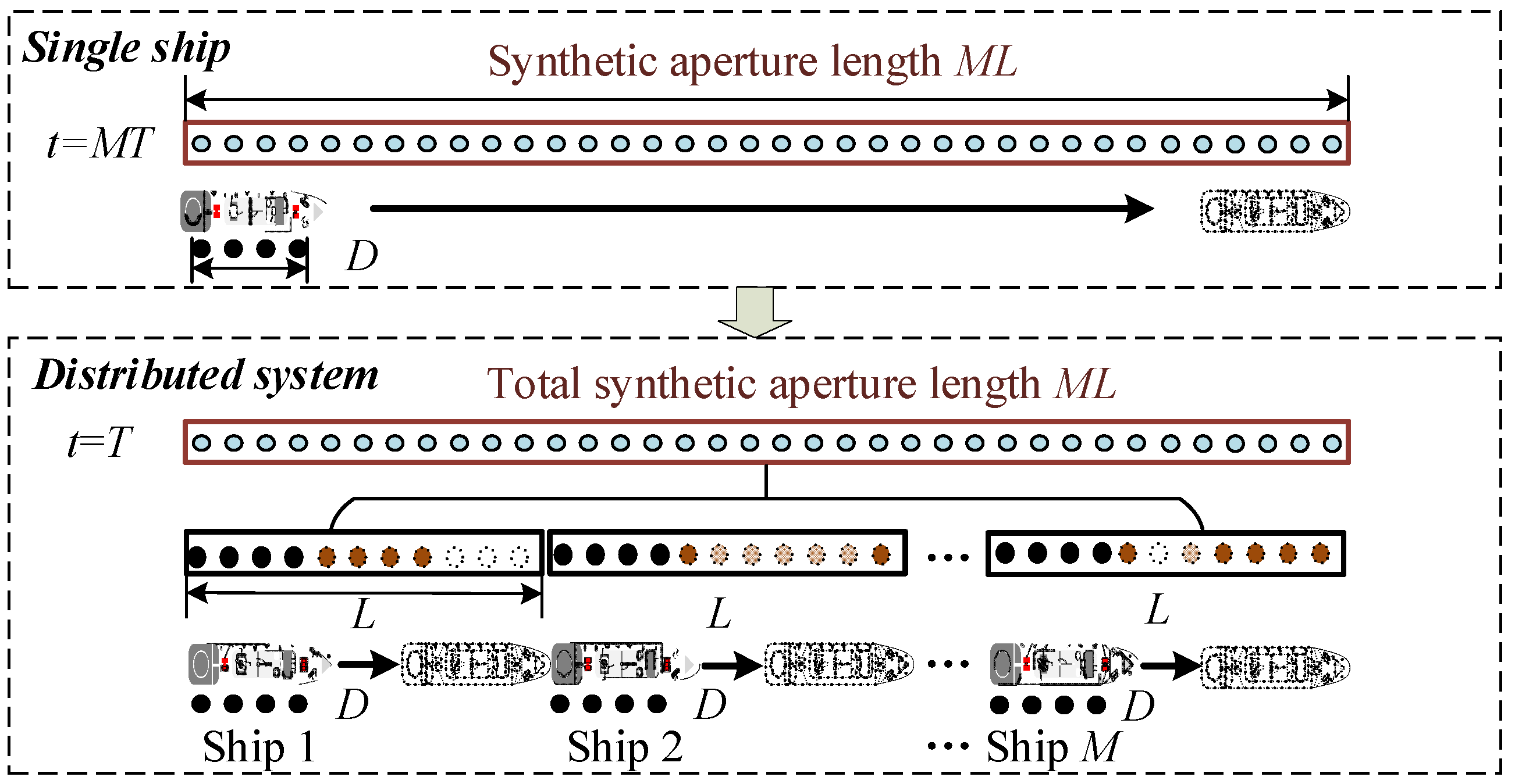
3. Azimuth Resolution Improvement Algorithm for the Distributed Shipborne HFHSSWR

The azimuth resolution improvement algorithm for the distributed shipborne HFHSSWR consists of two parts. First, the focused processing of the moving target echo for a single shipborne HFHSSWR is performed. The output is the two-dimension (2D) impulse response of the moving target, where the output over the azimuth frequency at the range of the target is the azimuth impulse response. Second, the azimuth impulse responses from multiple platforms are used as the input to the distributed synthetic aperture processing. The new azimuth impulse response with improved azimuth resolution is the final output.

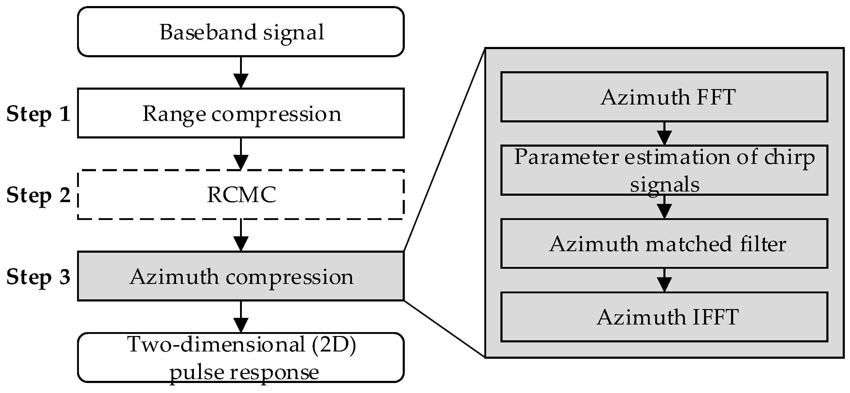
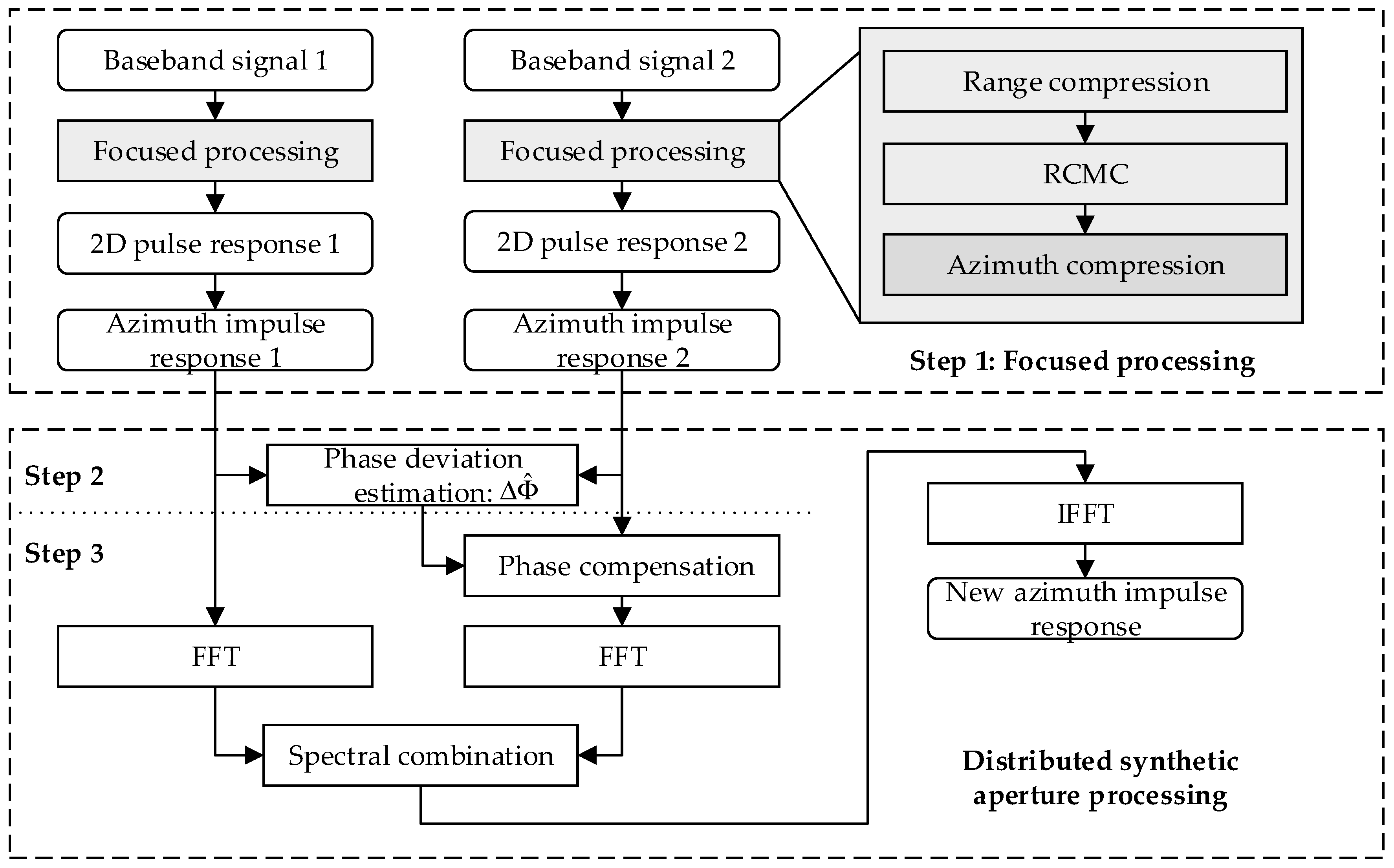
3.1. Focused Processing of the Moving Target Echo for a Single Shipborne HFHSSWR

Before spectral synthesis, the focused processing of the moving target echo for a single shipborne HFHSSWR is first performed based on the conventional range Doppler algorithm [19] and a focusing of the moving target. The moving target focusing is achieved by the parameter estimation of chirp signals [50,51,52], because the target motion causes the change in the initial azimuth frequency $f_{ac}$ and the azimuth FM rate $K_a$ of the signal in the azimuth direction. The block scheme of this processing is shown in Figure 5. The input signal of the algorithm is the demodulated baseband signal, see Equation (12). The focused processing consists of three steps as follows.

Step 1. Range compression.

For the baseband signal of Equation (12), the range matched filter can be expressed as [19]

$$h_r\left(\tau \right)=\mathrm{rect}\left(\frac{\tau }{T_r}\right)\exp \left\{-j\pi K_r{\tau }^2\right\}.$$

(18)

Then, the output of the range matched filter can be given by

$$\begin{array}{l}{s}_{rc}\left(\tau ,\eta \right)={\mathrm{IFFT}}_{\tau }\left\{{\mathrm{FFT}}_{\tau }\left[s_0\left(\tau ,\eta \right)\right]\cdot {\mathrm{FFT}}_{\tau }\left[h_r\left(\tau \right)\right]\right\}\\ \hspace{1em}\hspace{1em}\hspace{1em}=A_0{p}_r\left(\tau -\frac{d\left(\eta \right)}{c}\right){\omega }_a\left(\eta -{\eta }_c\right)\exp \left\{-j2\pi f_0\frac{d\left(\eta \right)}{c}\right\}\end{array}$$

(19)

where $p_r\left(\tau \right)$ is the compressed pulse envelope sinc function, $\mathrm{FFT}\left\{\cdot \right\}$ denotes the Fourier transform, and $\mathrm{IFFT}\left\{\cdot \right\}$ denotes the inverse Fourier transform. Next, the range equation $d_j\left(\eta \right)$ of the target T for $S_j$ is taken as an example to introduce the remaining steps of the focused processing.

Step 2. Range cell migration correction (RCMC).

From Equations (5) to (9), the amount of RCM to correct is given by

$$\begin{array}{l}\Delta d_j\left(\eta \right)=\left(\cos {\Delta }_i{v}_T\cos \theta +\left|{\mathit{v}}_T-{\mathit{v}}_j\right|\cdot \cos \alpha +2\sin {\Delta }_i{v}_1\right)\eta +\\ \hspace{1em}\hspace{1em}\hspace{1em}\left[-\frac{{\left(2\sin {\Delta }_i{v}_1+\cos {\Delta }_i{v}_T\cos \theta \right)}^2}{4r_1}+\frac{v_T{}^2+4v_1{}^2}{4r_1}+\frac{{\left|{\mathit{v}}_T-{\mathit{v}}_j\right|}^2{\sin }^2\alpha }{2r_j}\right]{\eta }^2\end{array}$$

(20)

Ignoring the ionospheric plasma motion velocity $v_1$, in the case of the low grazing angle ($\cos {\Delta }_i\approx 1$), Equation (20) can be simplified as

$$\Delta d_j\left(\eta \right)=\left(v_T\cos \theta +\left|{\mathit{v}}_T-{\mathit{v}}_j\right|\cdot \cos \alpha \right)\eta +\left[\frac{v_T{}^2{\sin }^2\theta }{4r_1}+\frac{{\left|{\mathit{v}}_T-{\mathit{v}}_j\right|}^2{\sin }^2\alpha }{2r_j}\right]{\eta }^2.$$

(21)

Considering the case of slow ship targets and the aperture time of 1–2 min, the quadratic term in Equation (21) can be ignored ($v_T$ is about 10 m/s, $r_j$ and $r_1$ can extend to a few hundred kilometers), and thus

$$\Delta d_j\left(\eta \right)\approx \left(v_T\cos \theta +\left|{\mathit{v}}_T-{\mathit{v}}_j\right|\cdot \cos \alpha \right)\eta \le \left(2v_T+v_j\right)\eta .$$

(22)

Therefore, the value of $\Delta d_j\left(\eta \right)$ may vary between several hundred meters and several thousand meters. Since an over-the-horizon radar typically has range resolutions of 5–10 km for ship-detection [37], the range migration could be neglected in most cases.

The correction of the range walk component of range migration can be considered for the target ship at high speeds and the spatial geometry of special propagation paths, and thus the output of the range matched filter can be modified as

$$s_{rc}\left(\tau ,\eta \right)={\mathrm{IFFT}}_{\tau }\left\{S_0\left(f_{\tau },\eta \right)H\left(f_{\tau }\right)\cdot \exp \left(j2\pi f_{\tau }\frac{\Delta d_{jl}\left(\eta \right)}{c}\right)\right\},$$

(23)

where $\Delta d_{jl}\left(\eta \right)=-\lambda f_{acj}\cdot \eta$.The signal applied range walk correction becomes

$$\begin{array}{l}{s}_{rc}\left(\tau ,\eta \right)=A_0{p}_r\left(\tau -\frac{d_{j0}}{c}\right){\omega }_a\left(\eta -{\eta }_{cj}\right)\hspace{1em}\times \\ \hspace{1em}\hspace{1em}\hspace{1em}\exp \left\{-j2\pi f_0\frac{d_{j0}}{c}\right\}\exp \left\{j2\pi f_{acj}\cdot \eta +j\pi K_{aj}{\eta }^2\right\}\end{array}$$

(24)

Step 3. Azimuth compression.

The initial azimuth frequency $f_{ac}$ and azimuth FM rate $K_a$ containing the parameters of the moving target cannot be calculated directly from system parameters. Hence, we adopt the Wigner-Hough transform (WHT) method [50,51] to estimate $f_{ac}$ and $K_a$. Assuming that $f_{acj}$ and $K_{aj}$ have been obtained, on the basis of Equation (24), the azimuth matched filter is

$$H_a\left(f_{\eta }\right)=\exp \left\{j\pi \frac{{\left(f_{\eta }-f_{acj}\right)}^2}{K_{aj}}\right\}.$$

(25)

The output of the compression can be given by [19]

$$\begin{array}{l}{s}_{ac}\left(\tau ,\eta \right)={\mathrm{IFFT}}_{\eta }\left\{{\mathrm{FFT}}_{\eta }\left[s_{rc}\left(\tau ,\eta \right)\right]\cdot H_a\left(f_{\eta }\right)\right\}\\ \hspace{1em}\hspace{1em}\hspace{1em}=A_0{p}_r\left(\tau -\frac{d_{j0}}{c}\right)p_{a_j}\left(\eta \right)\times \exp \left\{-j2\pi f_0\frac{d_{j0}}{c}\right\}\exp \left\{j2\pi f_{{\eta }_{cj}}\eta \right\}\end{array}$$

(26)

where $p_{a_j}\left(\eta \right)$ is the azimuth impulse response, $f_{{\eta }_{cj}}$ is the nonzero Doppler centroid. This output shows that the target is positioned at $\tau =d_{j0}/c$ and $\eta =0$.

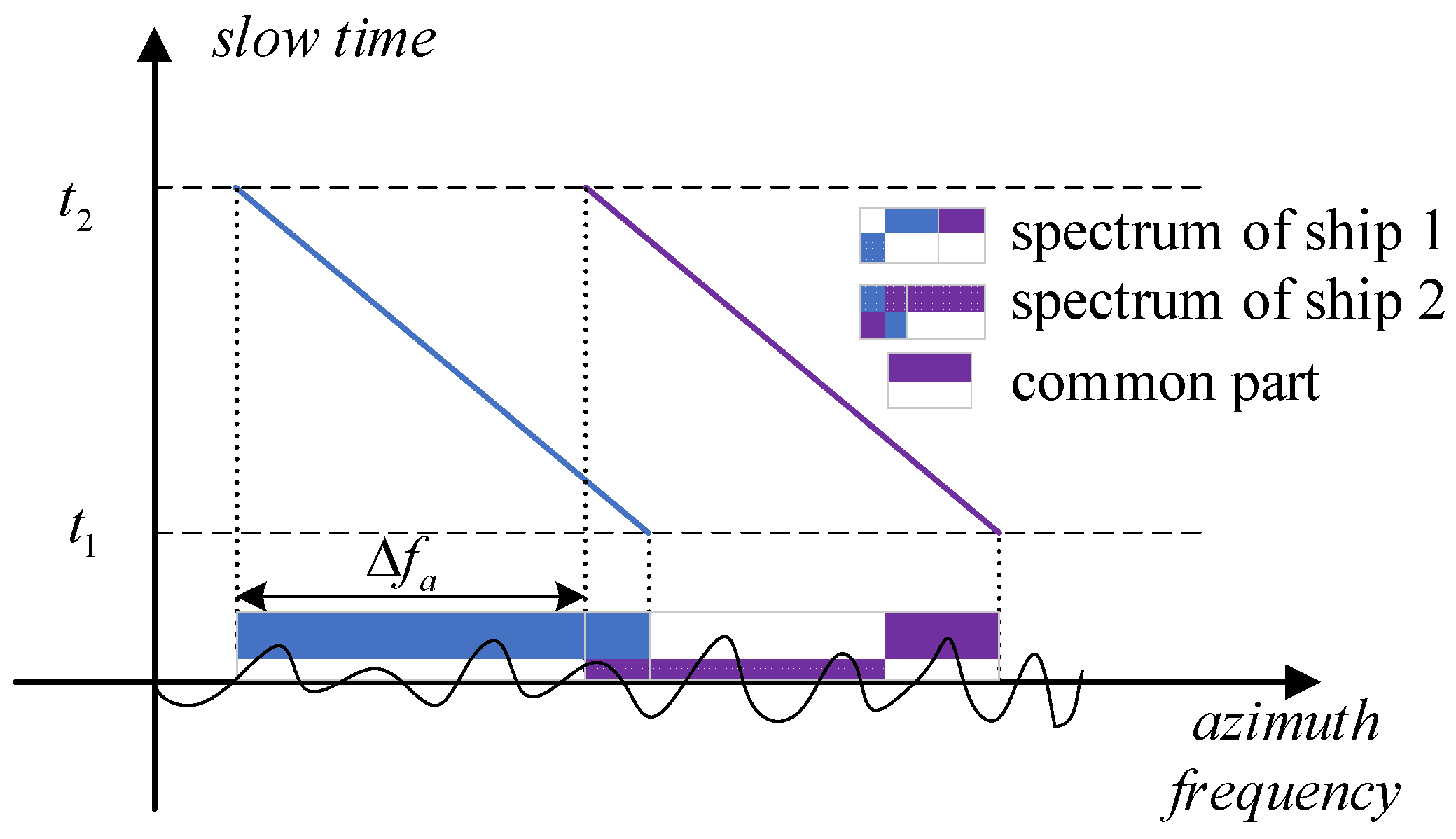
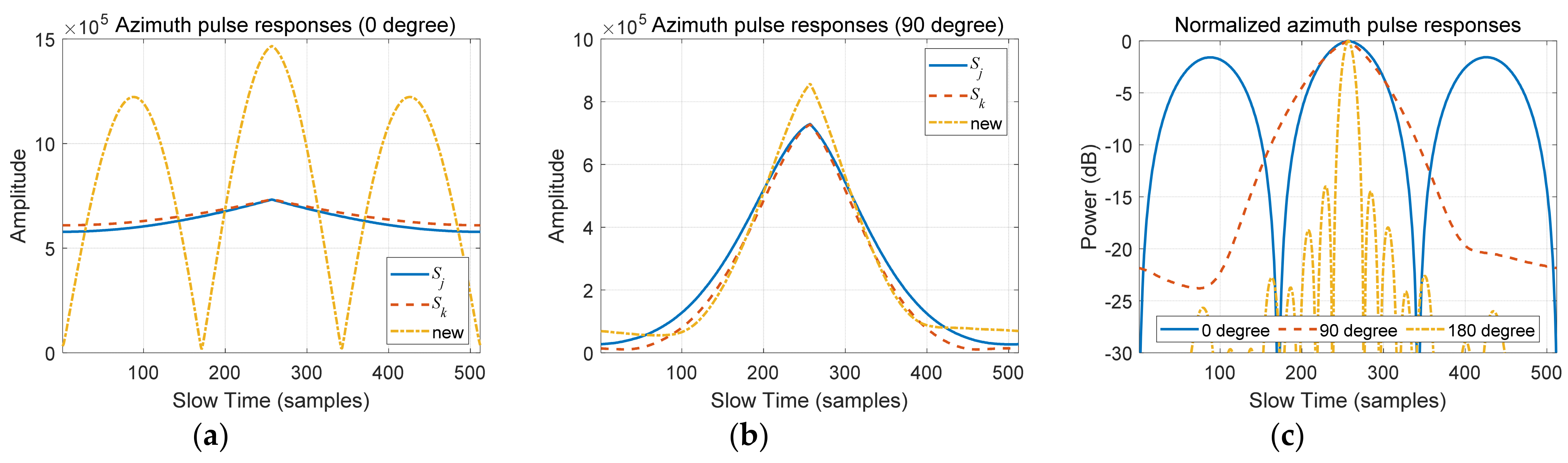
3.2. Distributed Synthetic Aperture Processing

As described earlier, the distributed synthetic aperture processing increases the azimuth bandwidth to improve the azimuth resolution of the distributed shipborne HFHSSWR system by spectral synthesis. The processing scheme needed to combine the azimuth spectra from different platforms is shown in Figure 6. This processing consists of three steps as follows.

Step 1. The moving target echoes from multiple platforms are focused separately (see Section 3.1).

Considering the case of two receiving ships $S_j$ and $S_k$, the system geometry is shown in Figure 3. According to Equation (26), the output of the focused processing over the azimuth frequency at the range of the target can be given by

$$s_{a_j}\left(\eta \right)=A_0{p}_{a_j}\left(\eta \right)\times \exp \left\{-j2\pi f_0\frac{d_{j0}}{c}\right\}\exp \left\{j2\pi f_{{\eta }_{cj}}\eta \right\},$$

(27)

$$s_{a_k}\left(\eta \right)=A_0{p}_{a_k}\left(\eta \right)\times \exp \left\{-j2\pi f_0\frac{d_{k0}}{c}\right\}\exp \left\{j2\pi f_{{\eta }_{ck}}\eta \right\}.$$

(28)

Step 2. Interferometric phase calculation.

On the basis of Equations (27) and (28), the constant phase shift between $s_{a_j}\left(\eta \right)$ and $s_{a_k}\left(\eta \right)$ is

$$\Delta \Phi =\frac{2\pi }{\lambda }\left(d_{k0}-d_{j0}\right).$$

(29)

The cross-correlation method [23] is used to estimate the phase deviation, which is expressed as

$$\Delta \widehat{\Phi }=\mathrm{angle}\left(\mathrm{E}\left\{\left[s_{a_j}\left(\eta \right)\cdot \exp \left(-j2\pi f_{{\eta }_{cj}}\eta \right)\right]\odot \mathrm{conj}\left[s_{a_k}\left(\eta \right)\cdot \exp \left(-j2\pi f_{{\eta }_{ck}}\eta \right)\right]\right\}\right).$$

(30)

Step 3. Spectral synthesis.

The phase compensation is first carried out for $s_{a_k}\left(\eta \right)$ utilizing the estimation of the phase shift, as given by

$$s_{{}_{a_k}}^1\left(\eta \right)=s_{a_k}\left(\eta \right)\cdot e^{i\Delta \Phi }=A_0{p}_{a_k}\left(\eta \right)\times \exp \left\{-j2\pi f_0\frac{d_{j_0}}{c}\right\}\exp \left\{j2\pi f_{{\eta }_{ck}}\eta \right\}.$$

(31)

Then, the spectral synthesis is performed by sum all spectrum data in the frequency domain. The combination of the two azimuth spectra is

$$S_{\mathrm{out}}\left(f_{\eta }\right)=S_j\left(f_{\eta }\right)H_1\left(f_{\eta }\right)+S_k^1\left(f_{\eta }\right)H_2\left(f_{\eta }\right),$$

(32)

where $S_j\left(f_{\eta }\right)=\mathrm{FFT}\left\{s_{a_j}\left(\eta \right)\right\}$, $S_k^1\left(f_{\eta }\right)=\mathrm{FFT}\left\{s_{{}_{a_k}}^1\left(\eta \right)\right\}$, $H_1\left(f_{\eta }\right)$ and $H_2\left(f_{\eta }\right)$ are the raised cosine filters for $S_j$ and $S_k^1$, respectively, to avoid abrupt phase changes at the boundary between the two azimuth spectra [33]. An inverse fast Fourier transform (IFFT) then completes the azimuth compression of the joined spectra:

$$s_{\mathrm{out}}\left(\eta \right)=\mathrm{IFFT}\left\{S_{\mathrm{out}}\left(f_{\eta }\right)\right\}=A\cdot p_{a_o}\left(\eta \right)\times \exp \left\{-j2\pi f_0\frac{d_{j_0}}{c}\right\}\exp \left\{j2\pi f_{{\eta }_{co}}\eta \right\},$$

(33)

where $p_{a_o}\left(\eta \right)$ is the azimuth impulse response of the new output, and will have a narrower main lobe width than $p_{a_j}\left(\eta \right)$ and $p_{a_k}\left(\eta \right)$ (see Equations (27) and (28)) of the respective platforms, due to the wider overall synthetic bandwidth. There are two exponential terms in Equation (33). The first one carries the inherent phase information of the target due to its group-range $d_{0j}$ at $\eta =0$. The second one is the linear phase term arising from the new nonzero Doppler centroid $f_{{\eta }_{co}}$ [19].

After performing all the steps above, the azimuth compressed data with improved azimuth resolution comes out. The azimuth resolution can be theoretically improved to n times when the synthetic bandwidth is increased by a factor of n.

4. Target Velocity Vector and Azimuth Parameters Inversion

This section is divided into two parts. In Section 4.1, a target parameters inversion method is proposed to estimate the azimuth angle and the velocity vector of the moving target, based on observations from different viewing angles of multiple platforms. In Section 4.2, the analysis on the azimuth inversion accuracy is described.

4.1. Target Parameters Inversion Method

The principal idea of the target parameters inversion method is to calculate the azimuth and the velocity vector of the moving target by solving the system of nonlinear equations between the target geometry and chirp signal parameters of moving target echoes from multiple platforms. This is because the chirp signal parameters ($f_{ac}$ and $K_a$) of the moving target echo contain the azimuth ${\alpha }_j$ and the velocity vector ${\mathit{v}}_T$ (with magnitude $v_T$ and direction ${\alpha }_{Tj}$) information of the target, according to Equations (8) and (9).

The target parameters inversion method includes two parts, considering two typical cases that the distributed system receives echo signals from two and three shipborne platforms.

The first part is the inversion method based on the echo signals from only two platforms. The two initial Doppler frequencies $f_{ac}$ and one FM rate $K_a$ are used to construct the system of nonlinear equations. It is worth noting that we use two initial Doppler frequencies instead of the two FM rates, because the expression of $f_{ac}$ is simpler than that of $K_a$, reducing the complexity of the equation system.

The second part considers the case of three platforms, where the system of nonlinear equations is constructed by using three initial Doppler frequencies $f_{ac}$. The target parameters inversion utilizing $f_{ac}$ measurements from multiple platforms will have higher reliability. This is because the azimuth frequency difference between two signals coming from two different platforms mainly arises from the difference of the initial Doppler frequency according to Equations (15) and (16), in addition to the advantage of the simpler expression of $f_{ac}$.

4.1.1. Target Parameters Inversion Based on the Echo Signals from Two Platforms

Considering the system geometry of two receiving ships $S_j$ and $S_k$, as shown in Figure 3, a system of nonlinear equations with regard to $f_{acj}$,$K_{aj}$ and $f_{ack}$ is established, called equation system 1 (ES-1). The ES-1 mainly consists of Equations (8), (9) and (A3), and includes the calculation formulas of certain parameters in ES-1 according to the system geometry. The complete system of equations is shown in Appendix B. The objective of this part is to invert the unknown target azimuth ${\alpha }_j$ and velocity vector ${\mathit{v}}_T$ by solving the ES-1 numerically.

The parameters contained in ES-1 are classified into three categories, according to known quantities, unknown quantities and functions of unknown quantities, see

Table 1. Types of parameters.

Types	Parameters
Known quantities	$h_0$, $v_1$, $L_j$, $d_{j0}$,${\alpha }_0$, $v_j$, $v_k$, $X$, ${\alpha }_d$
Unknown quantities	${\alpha }_j$, ${\alpha }_{Tj}$, $v_T$
Functions of unknown quantities	$r_j$, $r_T$, ${\beta }_j$, $r_1$, ${\Delta }_i$, $r_k$, ${\beta }_d$, ${\beta }_k$, ${\alpha }_{Tk}$, ${\alpha }_k$

. The known quantities can be accurately measured by radar systems and auxiliary equipment. The unknown quantities are the target azimuth ${\alpha }_j$ and the target velocity vector ${\mathit{v}}_T$. The functions of unknown quantities indicate that certain parameters can be computed from the unknown and known quantities.

As seen in Table 1, the ES-1 contains three unknowns quantities, ${\alpha }_j$, ${\alpha }_{Tj}$ and $v_T$. The number of equations in ES-1 would be equal to the number of unknowns quantities, after obtaining reliable estimates of the chirp signal parameters ($f_{acj}$,$K_{aj}$ and $f_{ack}$) of the echo signals from two platforms. Therefore, the target velocity vector and azimuth can be obtained by solving the ES-1 numerically.

4.1.2. Target Parameters Inversion Based on the Echo Signals from Three Platforms

On the basis of the system geometry corresponding to the ES-1, a third shipborne platform $S_l$ is considered. The platforms $S_j$, $S_k$ and $S_l$ are arranged sequentially along a straight line and sail along the same direction. The definition and the symbolic representation of the geometric parameters corresponding to $S_l$ are the same as those of $S_k$, except that the subscript is l. A new system of nonlinear equations with regard to $f_{acj}$, $f_{ack}$ and $f_{acl}$ is established, called ES-2, where the expressions of $f_{acj}$ and $f_{ack}$ are given by Equations (8) and (A3), respectively. In concert with $f_{ack}$, the expression of $f_{acl}$ can be derived as

$$f_{acl}=-\frac{1}{\lambda }\left[\cos {\Delta }_i\cdot v_T\cdot \cos \left({\alpha }_{Tl}-{\beta }_l\right)+\left(v_T\cdot \cos {\alpha }_{Tl}-v_l\cdot \cos {\alpha }_l\right)+2\sin {\Delta }_i\cdot v_1\right],$$

(34)

where $r_l=\sqrt{X_{kl}{}^2+r_k^2-2X{r}_k\cos {\alpha }_k}$, ${\beta }_{dl}=\mathrm{acos}\left(\frac{r_l{}^2+r_k{}^2-X_{kl}{}^2}{2r_l{r}_k}\right)$, ${\beta }_l={\beta }_k-{\beta }_{dl}$, ${\alpha }_{Tl}={\alpha }_{Tk}-{\beta }_{dl}$, ${\alpha }_{Tl}-{\beta }_l={\alpha }_{Tk}-{\beta }_k$, ${\alpha }_l={\alpha }_k-{\beta }_{dl}+{\alpha }_{dl}$, ${\alpha }_{dl}$ is the angular deviation between the directions of ${\mathit{v}}_k$ and ${\mathit{v}}_l$ (clockwise rotation angle from ${\mathit{v}}_k$ to ${\mathit{v}}_l$), and $X_{kl}$ is the distance between $S_k$ and $S_l$.

The ES-2 mainly consists of Equations (8), (A3) and (34), and includes the calculation formulas of certain parameters in ES-2. The complete system of equations is shown in Appendix B. The ES-2 contains all the parameters in Table 1 and the new parameters corresponding to $S_l$. However, the ES-2 still contains three unknown quantities, because all the new parameters can be expressed as the functions of the parameters in Table 1, when the position and motion state of $S_l$ are known. Hence, the target velocity vector and azimuth can also be obtained by solving the ES-2 numerically.

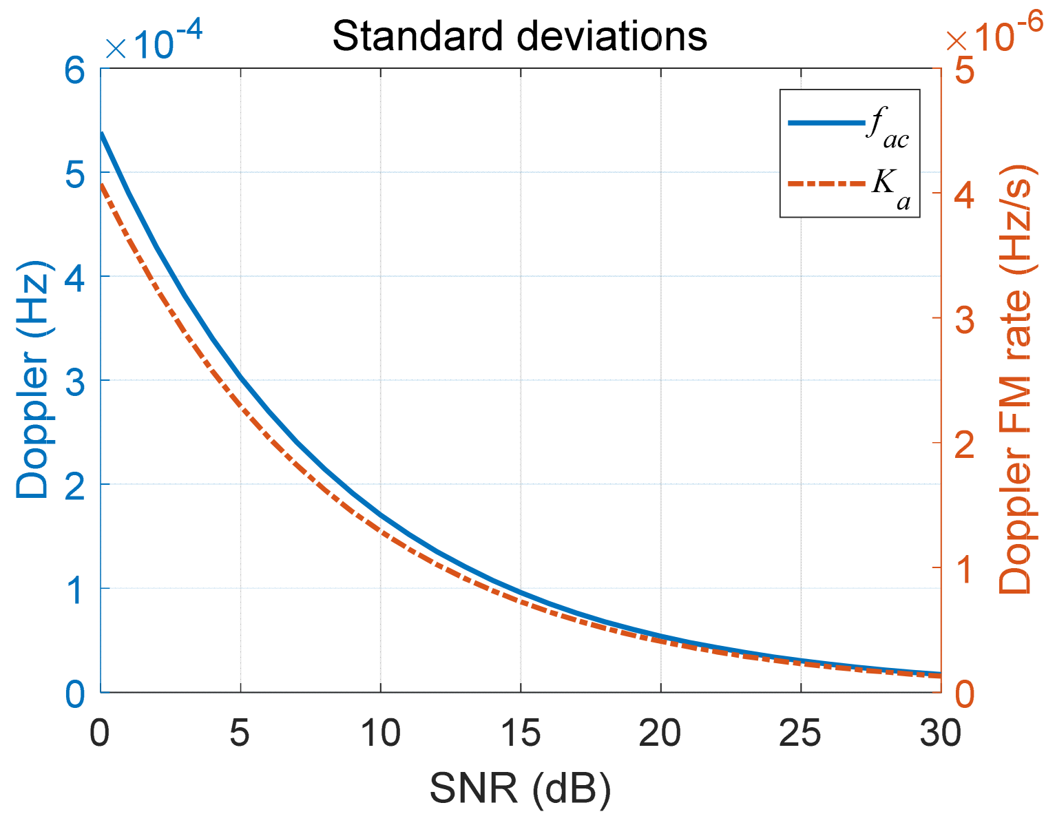
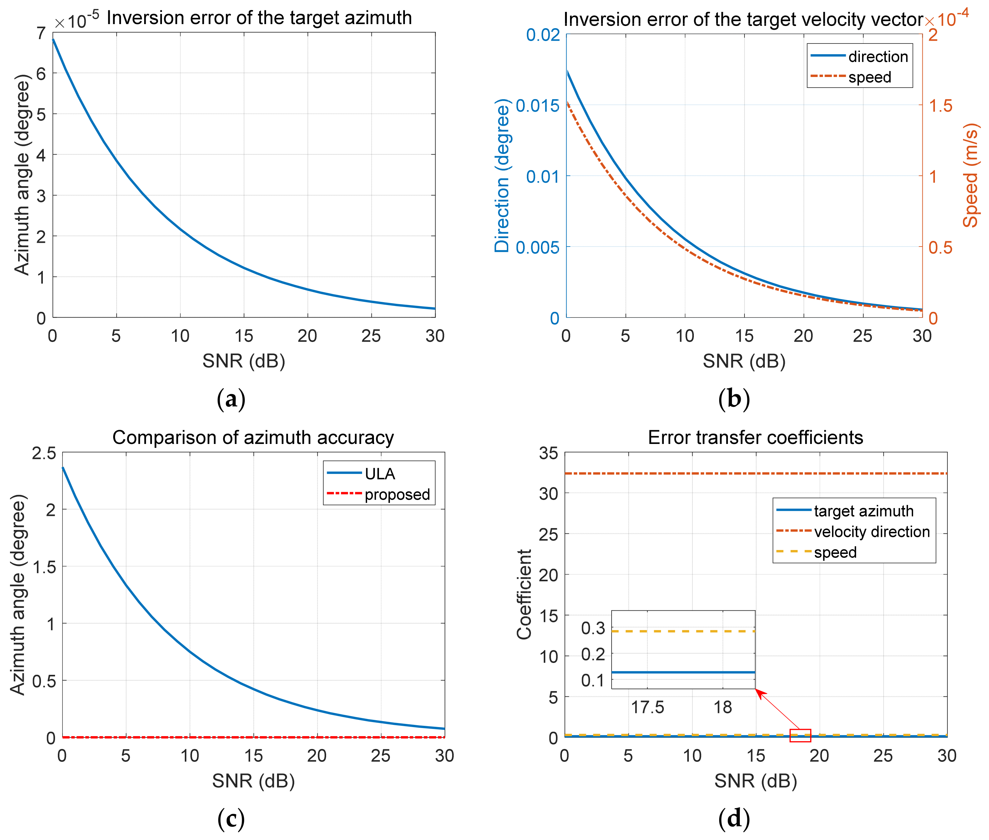
4.2. Analysis on the Azimuth Inversion Accuracy

The azimuth accuracy of the inversion method has been evaluated by an error propagation analysis of the method itself. The errors of the azimuth angle and the velocity vector arise from the propagation of the estimation errors of the chirp signal parameters $f_{ac}$ and $K_a$. This is because the method uses the chirp signal parameters measured directly to calculate the azimuth angle and the velocity vector of the moving target [53].

In this section, we only analyze the error propagation of the target azimuth. The derivation of the velocity vector error is similar to that of the azimuth error and is omitted. The azimuth error of inversion results caused by the estimation error of $f_{ac}$ in the ES-2 is evaluated as follows.

Let ${\alpha }_j=q\left(f_{acj},f_{ack},f_{acl}\right)$ (the closed-form solution of the azimuth angle ${\alpha }_j$ is not available) and suppose that $f_{acj}$, $f_{ack}$, $f_{acl}$ are measured with uncertainties $\delta f_{acj}$, $\delta f_{ack}$, $\delta f_{acl}$, which are independent and random. Then the variance of the estimates of ${\alpha }_j$ is [53]

$${\left(\delta \alpha \right)}^2={\left(\frac{\partial q}{\partial f_{acj}}\delta f_{acj}\right)}^2+{\left(\frac{\partial q}{\partial f_{ack}}\delta f_{ack}\right)}^2+{\left(\frac{\partial q}{\partial f_{acl}}\delta f_{acl}\right)}^2.$$

(35)

where the sensitivity coefficient $\partial q/\partial f_{ac}$ can be considered as a constant for a given system geometry and a specific target motion state, and the Cramer-Rao lower bound of $f_{ac}$ is given by [54,55]

$${\left(\delta f_{ac}\right)}^2=\mathrm{CRB}\left(f_{ac}\right)\approx \frac{6}{4{\pi }^2{N}^3{\Delta }^2{\mathrm{SNR}}_{\mathrm{in}}}=\frac{6}{4{\pi }^{2}N{T}_a{}^2{\mathrm{SNR}}_{\mathrm{in}}},$$

(36)

where N is the number of samples, $\Delta$ is the sampling interval, ${\mathrm{SNR}}_{\mathrm{in}}$ is the input Signal-to-Noise Ratios (SNR). For the sake of analysis, it is assumed that the echo signals in the azimuth direction of multiple platforms have the same input SNR, number of samples and aperture time. Thus, the variance can be expressed as

$${\left(\delta \alpha \right)}^2=\left(p_j+p_k+p_l\right)\cdot \mathrm{CRB}\left(f_{ac}\right)=p\frac{6}{4{\pi }^{2}N{T}_a{}^2{\mathrm{SNR}}_{\mathrm{in}}},$$

(37)

where $p_i={\left(\partial q/\partial f_{aci}\right)}^2$ and $p=p_j+p_k+p_l$, a constant for a given system geometry and a specific target motion state. According to Equation (14), the azimuth resolution is equal to the reciprocal of the azimuth bandwidth. Substituting Equation (14) into Equation (37), the expression of the variance follows

$${\left(\delta \alpha \right)}^2=\frac{6p{K}_a^2}{4{\pi }^{2}N\cdot {\mathrm{SNR}}_{\mathrm{in}}}\cdot {\rho }_a^2.$$

(38)

It can be seen in Equation (38) that the azimuth error $\delta \alpha$ of the inversion results is proportional to the azimuth resolution ${\rho }_a$. This indicates that the improvement of azimuth resolution can help to reduce the azimuth error of inversion results. It is worth noting that we only consider the effect of the estimation errors of the chirp signal parameters $f_{ac}$ and $K_a$, assuming that the geometric parameters are known quantities. These quantities also have measurement errors for practical application. The analysis of the corresponding error propagation is similar to the above derivation.

5. Simulation Experiments

In this section, some simulation experiments are performed to validate the proposed aperture synthesis processing techniques for the distributed shipborne HFHSSWR. This section is divided into two parts. In Section 5.1, the distributed synthetic aperture simulation is carried out based on the signal model described above. In Section 5.2, the target parameters inversions based on echo signals from two and three platforms are simulated separately.

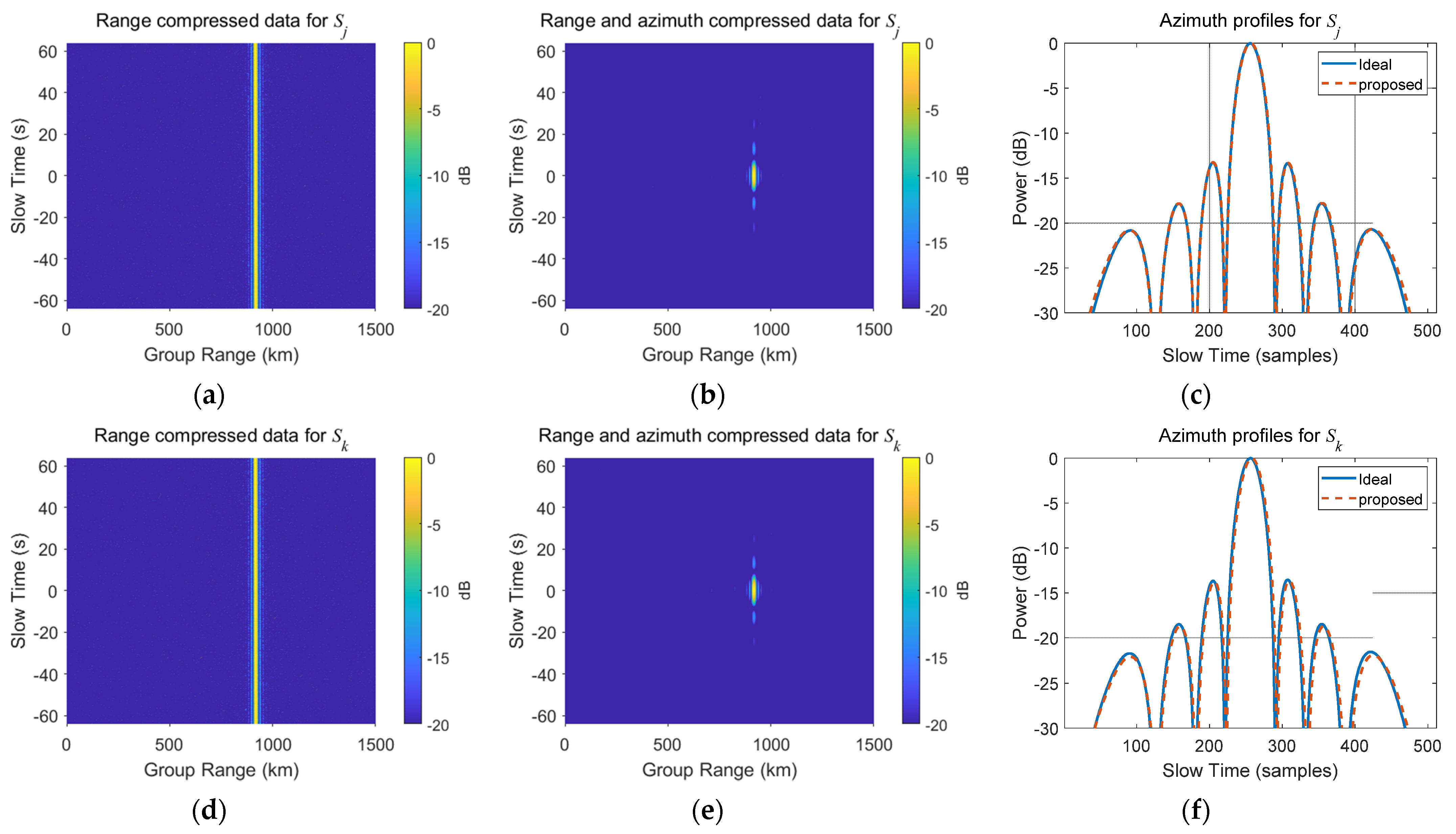
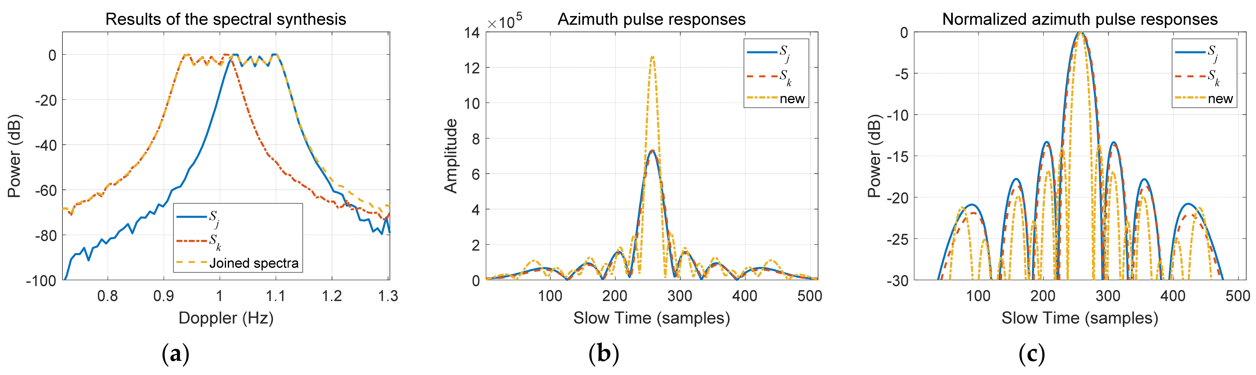
5.1. Distributed Synthetic Aperture Simulation

In this section, the distributed synthetic aperture simulation consists of two steps. First, the focused processing of the simulated echo signals for two ships is performed separately. Then, the distributed synthetic aperture processing is performed based on the output of the focused processing. The simulation considers the system geometry of two receiving ships and one ship target T. The system geometry lying in the ground plane is shown in Figure 7, where ship $S_k$ is north-east of ship $S_j$. The system parameters and the geometric parameters corresponding to two ships have been listed in

Table 2. System parameters.

Parameters	Values
Carrier frequency	20 MHz
Bandwidth	30 kHz
Sampling rate in range $f_s$	200 kHz
Pulse width $\tau$	0.01024 s
Pulse repeat frequency (PRF)	4 Hz
Coherent Integration Time (CIT)	128 s
Antenna aperture D	50 m
Input SNR	0 dB
Virtual height $h_0$	205 km
Vertical plasma motion velocity $v_1$	−10 m/s
Grazing angle ${\Delta }_i$	28.6 degree
Target speed $v_T$	15 m/s
Target velocity direction (North by East)	188 degree
Distance between $S_k$ and $S_j$	1920 m

and

Table 3. Geometric parameters associated with ships $S_j$ and $S_k$.

Parameters	$\mathbf{Values} \mathbf{of} {\mathit{S}}_{\mathit{j}}$	$\mathbf{Values} \mathbf{of} {\mathit{S}}_{\mathit{k}}$
Baseline length	700 km	-
Direction of the baseline $\overrightarrow{OS}$ (North by East)	68.7 degree	-
Direction of the vector $\overrightarrow{ST}$ (North by East)	97.5 degree	-
Distance from the target to the receiver	60 km	-
Speed of the receiving ship	15 m/s	15 m/s
Velocity direction (North by East)	8 degree	6.7 degree

, respectively. Following are the two steps to perform the distributed synthetic aperture simulation.

Step 1. The echo signals of two receiving ships are generated by applying the simulation parameters to the signal model described above, and then the focused processing of the echo signal for each platform is performed separately.

After the focused processing, the impulse responses of the moving target T for the receiving ships $S_j$ and $S_k$ are shown in Figure 8a–c and d–f, respectively. Figure 8a,d provide the range compressed data without RCMC before azimuth compression. The range compressed data over the azimuth frequency has migrated no more than one range cell. This is because the group-range of the target for ships $S_j$ and $S_k$ are accompanied by changes of 2.0 km and 1.9 km, respectively, which are less than a quarter of the range resolution 8.9 km. Consequently, the effect of RCM can be ignored.

Figure 8b,e illustrates the range and azimuth compressed point moving target T received by the two ships. These results are obtained by adopting the range Doppler algorithm based on the WHT method, a parameter estimation method for chirp signals [50,51]. The results of chirp signal parameter estimation for the echo signals from the two ships are given in

Table 4. Parameter estimation results of chirp signals.

Parameters		$\mathbf{Values} \mathbf{of} {\mathit{S}}_{\mathit{j}}$	$\mathbf{Values} \mathbf{of} {\mathit{S}}_{\mathit{k}}$
$f_{ac}$	theoretical value (Hz)	1.0551	0.9678
	estimated value (Hz)	1.0549	0.9674
	absolute error (Hz)	1.3631 × 10−4	4.4751 × 10−4
	relative error	0.01%	0.05%
$K_a$	theoretical value (Hz/s)	−9.7017 × 10−4	−9.5998 × 10−4
	estimated value (Hz/s)	−9.5998 × 10−4	−9.6866 × 10−4
	absolute error (Hz/s)	1.0190 × 10−5	8.6807 × 10−6
	relative error	1.05%	0.90%

. The relative errors of the initial frequency $f_{ac}$ and FM rate $K_a$ for both the ships $S_j$ and $S_k$ are in the order of 0.01% and 1%, respectively. This is because the values of $f_{ac}$ and $K_a$ are four and two orders of magnitude larger than the corresponding Cramer-Rao lower bounds of the WHT method for the two parameters, respectively.

Figure 8c,f shows comparisons of azimuth-compressed signals based on estimated parameters of the chirp signals and their theoretical values for the two ships. The peak-shifts of the azimuth profiles obtained after adopting the focused processing in Section 3.1 for $S_j$ and $S_k$ are 0.035 and 0.07 of the main lobe widths, respectively, which can be ignored. According to [54,55], we can further improve the parameter estimation accuracy of chirp signals, by increasing the number of samples and integration time, or selecting a parameter estimation method with higher accuracy, so as to obtain more accurate results in the focused processing of the moving target echo.

Step 2. The distributed synthetic aperture processing is applied to the azimuth-compressed signals of the moving target from the two receiving ships.

Figure 9a shows the results of the spectral synthesis and the original spectra for the echo signals in the azimuth direction received by the two shipborne platforms. It can be seen that the smoothed combination of the two spectra over the common part is achieved by using weighting filters. The synthetic bandwidth is increased by a factor of 1.7 compared with the azimuth bandwidth of the echo signal for ship $S_j$.

In Figure 9b, the new azimuth pulse response after the distributed synthetic aperture processing is shown and compared with the azimuth pulse responses of both the ships $S_j$ and $S_k$ in Figure 8c and Figure 8f, respectively. Figure 9c shows the normalized results of Figure 9b. As it is apparent, the azimuth resolution improvement is obtained.

To compare the azimuth resolution more clearly, the peak sidelobe ratio (PSLR), integrated sidelobe ratio (ISLR) and impulse response width (IRW) are used to quantitatively describe the performance of the proposed distributed synthetic aperture processing method. And

Table 5. Comparison results.

	PSLR (dB)	ISLR (dB)	IRW (Cells)
$S_j$	−13.30	−9.24	29.53
$S_k$	−13.71	−9.84	28.94
Distributed system	−13.65	−8.94	17.10

lists the corresponding calculation results of the azimuth pulse responses in Figure 9c. It can be seen from both Figure 9c and Table 5 that the PSLR and ISLR for the distributed shipborne HFHSSWR are basically consistent with those for a single shipborne HFHSSWR. And the azimuth resolution of the target T after the distributed synthetic aperture processing is improved by 1.7 times compared with that for ship $S_j$, which is consistent with the bandwidth enhancement ratio of 1.7.

Equally important, the peak level of the new azimuth pulse response for the distributed shipborne HFHSSWR system is 1.7 times higher than that for the system with a single receiving ship, i.e., the peak pulse power is increased by 4.8 dB, as shown in Figure 9b. Accordingly, the output SNR can be improved by 4.8 dB due to the increase in azimuth bandwidth. The improvement of SNR can help to increase the detection capabilities of the distributed radar system.

From the above analysis, the distributed radar system can achieve a higher azimuth resolution and a better target-detection performance than a single shipborne HFHSSWR utilizing the proposed azimuth resolution improvement algorithm.

5.2. Parameter Inversion Results

In this section, the simulations of the target velocity vector and azimuth parameters inversion based on echo signals from two and three platforms are conducted separately, to verify the effectiveness of the inversion method.

In the simulation process, we only consider the effect of the errors in the parameter estimation of chirp signals, ignoring the measurement errors of other geometric parameters. According to Equation (35), the accuracy of the target parameters inversion is determined by both the sensitivity coefficient and the estimation accuracy of the chirp signal parameters $f_{ac}$ and $K_a$. The expressions for the Cramer-Rao lower bounds of constant amplitude polynomial phase signals have been derived in [54,55], which depend on the input SNR, number of samples N and integration time $T_a$. Considering the simulation parameters in Table 2, the standard deviations of chirp signal parameters $f_{ac}$ and $K_a$ for the input SNR range of 0–30 dB are shown in Figure 10, and their maximum/minimum values are 5.3841 × 10⁻⁴/1.7026 × 10⁻⁵ Hz and 4.0727 × 10⁻⁶/1.2879 × 10⁻⁷ Hz/s, respectively.

Next, we will introduce the simulation process and results of the inversion method separately, and numerically analyze the effect of the estimation errors of $f_{ac}$ and $K_a$ in Figure 10 on the accuracy of the target parameters inversion.

5.2.1. Target Parameters Inversion Results for Two Ships

The main steps of the simulation are as follows. First, the errors shown in Figure 10 are added to the theoretical values of $f_{acj}$, $K_{aj}$, and $f_{ack}$. The system parameters and the geometric parameters for two ships utilized in the simulation are the same as those in Section 5.1, except that the angular deviation ${\alpha }_d$ is 0 and $v_k$ is equal to 12 m/s. Then, the ES-1 shown in with regard to $f_{acj}$, $K_{aj}$ and $f_{ack}$ is established, where the known quantities are replaced with the corresponding values and the unknown quantities are the target azimuth ${\alpha }_j$, the target speed $v_T$ and the target velocity direction ${\alpha }_{Tj}$. Finally, for the case of three equations and three unknowns, a numerical method (trust-region-dogleg algorithm [56]) is used to solve the system of nonlinear equations. The initial value of ${\alpha }_j$ is arbitrarily selected in the observed angular region $\left[-\pi /4,\pi /4\right]$. The initial values of $v_T$ and ${\alpha }_{Tj}$ are set to 10 m/s and 180 degrees (the entire angular region is $\left[0,2\pi \right]$).

To verify the accuracy of the inversion results, we first performed the target parameters inversion in the ideal case without the estimation errors of $f_{acj}$, $K_{aj}$, and $f_{ack}$. The absolute errors between the inversion results and the corresponding true values for target parameters ${\alpha }_j$, ${\alpha }_{Tj}$ and $v_T$ are shown in

Table 6. Absolute errors of the inversion results in the ideal case.

$$\begin{gathered} \mathbf{Initial} \mathbf{Value} \mathbf{of} {\mathit{\alpha }}_{\mathit{j}} \\ \left(\mathbf{Degree}\right) \end{gathered}$$	Target Azimuth (Degree)	Target Velocity Direction (Degree)	Target Speed (m/s)
45	1.7053 × 10−13	1.1369 × 10−13	8.8818 × 10−15
−45	1.7621 × 10−12	2.5580 × 10−13	8.5265 × 10−14

, which are in the order of 10⁻¹² degree, 10⁻¹³ degree and 10⁻¹⁴ m/s, respectively, and thus can be ignored. Then, the target parameters inversion considering the effect of the estimation errors of $f_{acj}$, $K_{aj}$, and $f_{ack}$ is performed by adopting the simulation steps described previously.

Figure 11a,b shows the inversion errors of three target parameters under the condition of the estimation errors of chirp signal parameters in Figure 10.

Table 7. Absolute errors of the inversion results considering the estimation errors of chirp signal parameters.

Input SNR (dB)	Target Azimuth (Degree)	Target Velocity Direction (Degree)	Target Speed (m/s)
0	3.6801 × 10−2	6.8546 × 10−2	6.4599 × 10−2
30	1.1624 × 10−3	2.1594 × 10−3	2.0414 × 10−3

lists the maximum and minimum values of the inversion errors for the input SNR range of 0–30 dB. The maximum values of the absolute errors of the target azimuth ${\alpha }_j$, the target speed $v_T$ and the target velocity direction ${\alpha }_{Tj}$ are in the order of 10⁻² degree, 10⁻² m/s and 10⁻² degree, respectively, which are much smaller than the corresponding true values. Figure 11c compares the azimuth estimation accuracy of the proposed method with that of a traditional ULA using a phase-based azimuth estimation method. The calculation of the latter is based on a 50 m long ULA of eight sensors and uses the main lobe beam width in the normal direction [36]. It can be seen from Figure 11c that the azimuth errors of the inversion results are smaller than the azimuth estimation error of the traditional ULA for the entire input SNR range of 0–30 dB. Moreover, the target velocity vector is not available for a single ship, so no comparison can be made.

As mentioned previously, the sensitivity coefficients $\partial q/\partial f_{dc}$ describe the sensitivity of the inversion results to uncertainty in each of the estimated parameters of the chirp signals. However, it is difficult to calculate the sensitivity coefficients separately because the closed-form solutions of the target parameters are not available. As an alternative, we calculated the ratio of the inversion error of the unknown target parameter and the estimation error of $f_{ac}$, called the error transfer coefficient, to easily observe the error propagation, as shown in Figure 11d. The error transfer coefficients can be considered as constants for a given system geometry and a specific target motion state. It can be seen from Figure 11d that the error transfer coefficient of the target azimuth is the smallest compared with those of the other two target parameters for the system parameters of this simulation, so the corresponding inversion error is also the smallest among the three target parameters.

5.2.2. Target Parameters Inversion Results for Three Ships

In this section, the system parameters and geometric parameters associated with ships $S_j$ and $S_k$ utilized in the simulation of the target parameters inversion for three ships are the same as those in Section 5.1. Additionally, the third shipborne platform $S_l$ moves in the same direction as $S_j$ and $S_k$ with a speed of 13 m/s. The distance between $S_k$ and $S_l$ is 1920 m, and ship $S_l$ is north-east of ship $S_k$. The simulation steps and initial values of the unknown target parameters are the same as those in Section 5.2.1, except that the ES-2 is used for calculation.

The absolute errors of the target parameters ${\alpha }_j$, ${\alpha }_{Tj}$ and $v_T$ in the ideal case for the ES-2 are in the order of 10⁻¹² degree, 10⁻¹³ degree and 10⁻¹³ m/s, respectively, which can be ignored.

Table 8. Absolute errors of the inversion results for the ES-2.

Input SNR (dB)	Target Azimuth (Degree)	Target Velocity Direction (Degree)	Target Speed (m/s)
0	6.8355 × 10−5	1.7437 × 10−2	1.5230 × 10−4
30	2.1616 × 10−6	5.5139 × 10−4	4.8376 × 10−6

and Figure 12 show the inversion errors of the target parameters for the ES-2. It can be seen that for the entire input SNR range of 0–30 dB, the inversion errors of the three target parameters for the ES-2 are all smaller than those for the ES-1.

Specifically, the azimuth estimation accuracy for the system with three receiving ships is three orders of magnitude higher than that for the system with two receiving ships. This is because the error transfer coefficients of the three target parameters for the ES-2 are much lower than those for the ES-1 in Figure 11d. In particular, the error transfer coefficient of the target azimuth for the ES-2 is less than one, which allows the corresponding inversion error of the target azimuth to be as small as the estimation errors of $f_{ac}$.

Similarly, the error reduction of ${\alpha }_{Tj}$ and $v_T$ for the system with three ships arises from the decrease in the corresponding error transfer coefficients, compared with that for the system with two ships. For the target velocity direction ${\alpha }_{Tj}$, the coefficient decreases by a factor of 3.9, so the improvement of the velocity direction error is not significant compared with that of the speed error.

Overall, the increase of the number of shipborne platforms in the distributed shipborne HFHSSWR system is beneficial for improving the accuracy of the target parameters inversion.

In summary, the multi-angle observations from different shipborne platforms provide more comprehensive target information consisting of target velocity vector and azimuth parameters. The target velocity vector and azimuth can be obtained by the parameters inversion only with the observations of two platforms when the system parameters (see Table 1) and partial ionospheric parameters ($h_0$ and $v_1$) are known. The observations of three or more platforms can further improve the inversion accuracy of target information.

6. Discussion

This study aims at improving the azimuth resolution of the distributed shipborne HFHSSWR by using a spectral synthesis method. The simulated results in Section 5 show that the azimuth resolution and the out SNR of the target T after the distributed synthetic aperture processing are improved by 1.7 times and 4.8 dB compared with those for the system with a single receiving ship, respectively. Therefore, the distributed shipborne HFHSSWR can achieve a higher azimuth resolution and a better target-detection performance than a single shipborne HFHSSWR. Additionally, owing to the distributed observations from different viewing angles, this system can also obtain a higher azimuth estimation accuracy than a single shipborne HFHSSWR with uniform linear array (ULA), and the estimation of the target velocity vector that is not available for a single shipborne HFHSSWR, by utilizing the target parameters inversion. As a result, the distributed shipborne HFHSSWR can break through the limitation of the small array aperture of a single shipborne HFHSSWR, utilizing the distributed aperture synthesis processing.

Despite these encouraging results, there are a few obvious questions and limitations of the developed model and algorithms, which are discussed below.

The first limitation is the assumption of a quiet ionosphere and shipborne platforms with uniform linear motion. This limits the scope of application of the developed model and two algorithms. Under the assumption of a quiet ionosphere, the ionosphere only causes the variation of the group-range, which ignores its effect on the phase of echo signals. However, the phase of the echo signals under non-stationary ionospheric conditions will be affected by a phase modulation and random perturbations [3,41,42,43,44,45], so perturbation correction methods [5,57] are needed to improve the performance of algorithms. Moreover, ionospheric parameters vary during the day, year, and solar cycle, which affects variations in signal propagation in the ionosphere. Therefore, we need to evaluate the signal propagation by the real-time monitoring of the ionosphere with auxiliary equipment, such as oblique sounders. On the other hand, under the assumption of shipborne platforms with uniform linear motion, the effect of the non-ideal motion of shipborne platforms is ignored, which is applicable in low sea states. However, in severe sea states the non-ideal motion of shipborne platforms results in non-negligible additional peaks in Doppler spectra [46,47,48,49], but for known motion, the corresponding correction can be made. Therefore, future work will extend the model and algorithms to non-stationary ionospheric conditions and the case of the non-ideal motion, to improve the applicability of this work.

Second, the target motion state limits the scope of application of the azimuth resolution improvement algorithm. The simulation in Section 5.1 assumes that the target and the receiving ships move in opposite directions. In this case, the maximum azimuth resolution can be achieved. However, the azimuth resolution obtained by the aperture synthesis processing is greatly reduced when the receiving ships move in the same direction as the target’s movement, especially for the case when the target and the receiving ships move at similar speeds.

To explain this more clearly, Figure 13 shows the comparison of the final azimuth impulse responses for three typical cases, where the angles between the velocity direction of the receiving ship $S_j$ and that of the target are 180, 90 and 0 degree, corresponding to Case 1, Case 2 and Case 3, respectively. The simulation parameters are the same as those in Section 5.1, except that the vertical plasma motion velocity $v_1$ is zero. The angular deviation ${\alpha }_d$ between the directions of ${\mathit{v}}_j$ and ${\mathit{v}}_k$ is −1.3 degree. The direction of the position vector from $S_j$ to $S_k$ is the same as that of ${\mathit{v}}_j$. The results and conclusions for Case 1 are basically consistent with those of Section 5.1. For Case 2, the final azimuth resolution and peak pulse power are improved by 1.2 times and 1.4 dB compared with those for the ship $S_j$, respectively, which are consistent with the bandwidth enhancement ratio of 1.2. For Case 3, the grating lobes appear in the final azimuth impulse response. This is because the azimuth bandwidths of the ships $S_j$ and $S_k$ are so narrow that the combined spectrum is noncontiguous. The final impulse response widths for cases 1, 2 and 3 are 16.28, 80.48 and 79.33 cells, respectively. The final azimuth impulse response for Case 1 has the narrowest main lobe. The main lobe width for Case 3 is smaller than that of Case 2, because the spectral shift between the azimuth spectra of the ships $S_j$ and $S_k$ for Case 3 is larger than the synthetic bandwidth for Case 2.

Over all, as the angle between ${\mathit{v}}_T$ and ${\mathit{v}}_j$ changes from 180 degree to 0 degree, the azimuth bandwidths of $S_j$ and $S_k$ become smaller, resulting in a lower azimuth resolution. Meanwhile, the gaps between the azimuth spectra from different platforms appear, leading to the appearance of grating lobes. Therefore, the antenna array with a certain aperture size is still required for each receiving ship in the distributed shipborne HFHSSWR system as a necessary complement.

Furthermore, the accuracy of the target parameters inversion method is affected by the error transfer coefficient, which depends on the system geometry and the system parameters. In Section 5.2, the error transfer coefficients corresponding to the simulation are small. As a result, the errors of the inversion results caused by the estimation errors of the initial frequency $f_{ac}$ and the FM rate $K_a$ are much lower than the corresponding true values. However, for some specific values of geometry parameters, the error transfer coefficients may be so large that the azimuth error of the inversion results of the distributed shipborne HFHSSWR system is larger than the azimuth estimation error of a ULA with small aperture on a single platform, which is more likely to occur for the equation system 1. In addition, the inversion method requires the high measurement accuracy of the system parameters. Therefore, the error transfer coefficient should be taken into account in the process of constructing the equation system for the target parameters inversion. This process requires selecting the appropriate combination of platforms to reduce the error transfer coefficient.

7. Conclusions

In this paper, we describe the aperture synthesis processing techniques for the distributed shipborne HFHSSWR system, with the goal of azimuth resolution improvement and obtaining the velocity vector and the azimuth estimation of the moving target. This study consists of three aspects.

First, we build a baseband signal model of the moving target for the distributed shipborne HFHSSWR system. The model indicates that the echo signals in the azimuth direction of multiple platforms show relative spectral shifts, arising from the difference in viewing angle. Moreover, the maximum length of the synthetic aperture is not available due to the limited aperture time and slow ship speeds in a shipborne HFHSSWR system. Therefore, the azimuth resolution can be improved by combining the azimuth spectra from different platforms.

Second, an azimuth resolution improvement algorithm for the distributed shipborne HFHSSWR system is presented. The algorithm is based on the spectral shift principle, in which all the information in echo signals of the moving target from different platforms is used to increase the azimuth resolution. The simulation takes into account the basic case of two receiving ships which move opposite to the velocity direction of the target. The results show that the azimuth resolution of the distributed radar system is improved by 1.7 times compared with that of a single shipborne HFHSSWR, which demonstrates the effectiveness of the proposed approach for the moving target. Specifically, the output SNR of the target for the distributed radar system is increased by 4.8 dB, which can also help to obtain a better target-detection performance. However, it is worth noting that the synthetic aperture processing yields little or no resolution improvement in azimuth direction when the receiving ships move in the same direction as the target’s movement. This is because the synthetic aperture technique depends on the motion of receiving platforms relative to the target.

Finally, we present a target azimuth and velocity vector parameters inversion method. The method establishes the equation systems 1 and 2 for the unknown target parameters, by utilizing the multi-angle observations of the moving target provided by two and three receiving ships, respectively, to obtain the numerical solutions of the target parameters. The simulation shows that employing the inversion method, the target velocity vector and the high-precision estimation of the target azimuth can be obtained.

The proposed signal model and the aperture synthesis processing techniques for the distributed shipborne HFHSSWR system can not only improve the limited azimuth resolution and azimuth estimation accuracy of a single shipborne HFHSSWR, but also obtain the target velocity vector that cannot be obtained by the single radar system, which is of great importance to improve the performance of this distributed radar system. Future work will consider the effects of non-stationary ionospheric conditions and the case of the non-ideal motion, to improve the applicability of the proposed model and techniques.

References

1. Zhou, X.; Wei, Y.; Liu, Y. Broadened Sea Clutter Suppression Method for Shipborne HF Hybrid Sky-Surface Wave Radar. In Proceedings of the 2020 IEEE Radar Conference (RadarConf20), Florence, Italy, 21–25 September 2020. [Google Scholar]
2. Zhu, Y.; Wei, Y.; Yu, L. Ionospheric Decontamination for HF Hybrid Sky-Surface Wave Radar on a Shipborne Platform. IEEE Geosci. Remote Sens. Lett. 2017, 14, 2162–2166. [Google Scholar] [CrossRef]
3. Wei, Y.; Zhu, Y. Simulation Study of First-Order Sea Clutter Doppler Spectra for Shipborne High Frequency Radar via Hybrid Sky-Surface Wave Propagation. J. Appl. Remote Sens. 2017, 11, 014001. [Google Scholar] [CrossRef]
4. Anderson, S. Bistatic and Stereoscopic Configurations for HF Radar. Remote Sens. 2020, 12, 689. [Google Scholar] [CrossRef] [Green Version]
5. Zhou, Q.; Yue, X.; Zhang, L.; Wu, X.; Wang, L. Correction of Ionospheric Distortion on HF Hybrid Sky-Surface Wave Radar Calibrated by Direct Wave. Radio Sci. 2019, 54, 380–396. [Google Scholar] [CrossRef]
6. Ding, M.; Wei, Y.; Yu, L.; Tong, P. Adaptive Suppression of Main-Lobe Spread Doppler Clutter with High Directivity for HFSSWR Using Oblique Projection. Electron. Lett. 2019, 55, 1245–1247. [Google Scholar] [CrossRef]
7. Yang, L.-Q.; Fan, J.-M.; Guo, L.-X.; Liu, W.; Li, X.; Feng, J.; Lou, P.; Lu, Z.-X. Simulation Analysis and Experimental Study on the Echo Characteristics of High-Frequency Hybrid Sky–Surface Wave Propagation Mode. IEEE Trans. Antennas Propag. 2018, 66, 4821–4831. [Google Scholar] [CrossRef]
8. Wei, Y.; Tong, P.; Xu, R.; Yu, L. Experimental Analysis of a HF Hybrid Sky-Surface Wave Radar. IEEE Aerosp. Electron. Syst. Mag. 2018, 33, 32–40. [Google Scholar] [CrossRef]
9. Li, M.; Zhang, L.; Wu, X.; Yue, X.; Emery, W.J.; Yi, X.; Liu, J.; Yang, G. Ocean Surface Current Extraction Scheme With High-Frequency Distributed Hybrid Sky-Surface Wave Radar System. IEEE Trans. Geosci. Remote Sens. 2018, 56, 4678–4690. [Google Scholar] [CrossRef]
10. Ji, Y.; Zhang, J.; Chu, X.; Wang, Y.; Yang, L. Ocean Surface Current Measurement with High-Frequency Hybrid Sky–Surface Wave Radar. Remote Sens. Lett. 2017, 8, 617–626. [Google Scholar] [CrossRef]
11. Cui, X.; Gong, W.; Ye, X.; Pan, L.; Chen, Y. Application of Wuhan Ionospheric Oblique Backscattering Sounding System (WIOBSS) for Sea-State Detection. IEEE Geosci. Remote Sens. Lett. 2016, 13, 389–393. [Google Scholar] [CrossRef]
12. Chen, S.; Huang, W.; Gill, E.W. First-Order Bistatic High-Frequency Radar Power for Mixed-Path Ionosphere-Ocean Propagation. IEEE Geosci. Remote Sens. Lett. 2016, 13, 1940–1944. [Google Scholar] [CrossRef]
13. Chen, S.; Gill, E.W.; Huang, W. A First-Order HF Radar Cross-Section Model for Mixed-Path Ionosphere–Ocean Propagation With an FMCW Source. IEEE J. Ocean. Eng. 2016, 41, 982–992. [Google Scholar] [CrossRef]
14. Walsh, J.; Gill, E.W.; Huang, W.; Chen, S. On the Development of a High-Frequency Radar Cross SectionModel for Mixed Path Ionosphere–Ocean Propagation. IEEE Trans. Antennas Propag. 2015, 63, 2655–2664. [Google Scholar] [CrossRef]
15. Zhao, Z.; Wan, X.; Zhang, D.; Cheng, F. An Experimental Study of HF Passive Bistatic Radar Via Hybrid Sky-Surface Wave Mode. IEEE Trans. Antennas Propag. 2013, 61, 415–424. [Google Scholar] [CrossRef]
16. Riddolls, R.J. Limits on the Detection of Low-Doppler Targets by a High Frequency Hybrid Sky-Surface Wave Radar System. In Proceedings of the 2008 IEEE Radar Conference, Rome, Italy, 26–30 May 2008. [Google Scholar]
17. Melyanovcky, P.A.; Turgenev, I.S. Bistatic HF Radar for Oceanography Applications with the Use of Both Ground and Space Waves. Telecommun. Radio Eng. 1997, 51, 73–80. [Google Scholar] [CrossRef]
18. Martino, G.D.; Iodice, A. Maritime Surveillance with Synthetic Aperture Radar; Institution of Engineering and Technology: London, UK, 2020; ISBN 978-1-78561-602-0. [Google Scholar]
19. Cumming, I.G.; Wong, F.H. Digital Processing of Synthetic Aperture Radar Data: Algorithms and Implementation; Artech House: Boston, MA, USA, 2005; ISBN 978-1-58053-058-3. [Google Scholar]
20. Carrer, L.; Zancanella, F.; Bruzzone, L. Mars HF Surface Imaging by Processing SHARAD Off-Nadir Echoes. In Proceedings of the EPSC-DPS Joint Meeting 2019, Geneva, Switzerland, 15–20 September 2019; Volume 13. [Google Scholar]
21. Kobayashi, T.; Ono, T. SAR/InSAR Observation by an HF Sounder. J. Geophys. Res. Planets 2007, 112, E03S90. [Google Scholar] [CrossRef] [Green Version]
22. Chen, J.; Li, Z.; Li, C.; Zhou, Y. Signal Processing Algorithm of Spaceborne SIMO HF-SAR for Three-Dimensional Topside Ionosphere Exploration. In Proceedings of the 2009 5th International Conference on Wireless Communications, Networking and Mobile Computing, Beijing, China, 24–26 September 2009. [Google Scholar]
23. Li, L.; Li, F. Ionosphere Tomography Based on Spaceborne SAR. Adv. Space Res. 2008, 42, 1187–1193. [Google Scholar] [CrossRef]
24. Ding, F.; Zhao, C.; Chen, Z.; Li, J. Sea Echoes for Airborne HF/VHF Radar: Mathematical Model and Simulation. Remote Sens. 2020, 12, 3755. [Google Scholar] [CrossRef]
25. Voronovich, A.; Zavorotny, V. An Evaluation of the HF/VHF Synthetic Aperture Radar System for Ocean Wave Spectra Measurement. In Proceedings of the 2017 IEEE International Geoscience and Remote Sensing Symposium (IGARSS), Fort Worth, TX, USA, 23–28 July 2017; pp. 1530–1533. [Google Scholar]
26. Peng, H.; Xue, W.; Zhu, S.; Yu, G. An Improved Model of HF-SAR for Estimating Surface Current Velocity. In Proceedings of the 2007 1st Asian and Pacific Conference on Synthetic Aperture Radar, Huangshan, China, 5–9 November 2007; pp. 760–765. [Google Scholar]
27. Xue, W.; Zhang, M.; Tang, J.; Han, S. Surface Current Extraction by Onboard High Frequency SAR. In Proceedings of the TENCON 2006–2006 IEEE Region 10 Conference, Hong Kong, China, 14–16 November 2006. [Google Scholar]
28. Nithirochananont, U.; Antoniou, M.; Cherniakov, M. Passive Coherent Multistatic SAR Using Spaceborne Illuminators. IET Radar Sonar Navig. 2020, 14, 628–636. [Google Scholar] [CrossRef]
29. Wojaczek, P.; Cristallini, D. Optimal Trajectories for Range Resolution Improvement in Multi-PCL SAR. AEU-Int. J. Electron. Commun. 2017, 73, 173–182. [Google Scholar] [CrossRef]
30. Xu, H.; Wang, J.; Yuan, J.; Wang, R.; Shan, X. Range-Resolution Improvement for Spaceborne/Airborne Bistatic Synthetic Aperture Radar Using Stepped-Frequency Chirp Trains. IET Signal Process. 2015, 9, 377–386. [Google Scholar] [CrossRef]
31. Zhao, B.; Liu, M.; Lu, X.; Li, C.; Wang, P. High Resolution Imaging on Distributed SAR Using Joint Space-Time-Frequency Method. In Proceedings of the 2014 12th International Conference on Signal Processing (ICSP), Hangzhou, China, 19–23 October 2014; pp. 330–335. [Google Scholar]
32. Cristallini, D.; Pastina, D.; Lombardo, P. Exploiting MIMO SAR Potentialities With Efficient Cross-Track Constellation Configurations for Improved Range Resolution. IEEE Trans. Geosci. Remote Sens. 2011, 49, 38–52. [Google Scholar] [CrossRef]
33. Guillaso, S.; Reigber, A.; Ferro-Famil, L.; Pottier, E. Range Resolution Improvement of Airborne SAR Images. IEEE Geosci. Remote Sens. Lett. 2006, 3, 135–139. [Google Scholar] [CrossRef]
34. Marechal, R.; Amiot, T.; Attia, S.; Aguttes, J.-P.; Souyris, J.-C. Distributed SAR for Performance Improvement. In Proceedings of the 2005 IEEE International Geoscience and Remote Sensing Symposium, IGARSS ’05, Seoul, Korea, 29 July 2005; Volume 2, pp. 1030–1033. [Google Scholar]
35. Prati, C.; Rocca, F. Improving Slant-Range Resolution with Multiple SAR Surveys. IEEE Trans. Aerosp. Electron. Syst. 1993, 29, 135–143. [Google Scholar] [CrossRef]
36. Richards, M.A. Fundamentals of Radar Signal Processing, 2nd ed.; McGraw-Hill Education: New York, NY, USA, 2014; ISBN 978-0-07-179832-7. [Google Scholar]
37. Fabrizio, G.A. High Frequency Over-The-Horizon Radar: Fundamental Principles, Signal Processing, and Practical Applications; McGraw-Hill Education: New York, NY, USA, 2013; ISBN 978-0-07-162127-4. [Google Scholar]
38. Harris, T.J.; Cervera, M.A.; Pederick, L.H.; Quinn, A.D. Separation of O/X Polarization Modes on Oblique Ionospheric Soundings. Radio Sci. 2017, 52, 1522–1533. [Google Scholar] [CrossRef] [Green Version]
39. Gething, P.J.D. Relation between Oblique and Ground Path-Lengths in Ionospheric Propagation over a Curved Earth. Nature 1962, 193, 260–261. [Google Scholar] [CrossRef]
40. Breit, G.; Tuve, M.A. A Test of the Existence of the Conducting Layer. Phys. Rev. 1926, 28, 554–575. [Google Scholar] [CrossRef]
41. Ding, M.; Tong, P.; Wei, Y.; Yu, L. Multiple Phase Screen Modeling of HF Wave Field Scintillations Caused by the Irregularities in Inhomogeneous Media. Radio Sci. 2021, 56, e2020RS007239. [Google Scholar] [CrossRef]
42. Zernov, N.; Gherm, V.; Zaalov, N. High-Frequency EM Wave Field Propagation in the Disturbed Ionosphere: Review of Recent Research at St. Petersburg State University. In Proceedings of the 2019 Russian Open Conference on Radio Wave Propagation (RWP), Kazan, Russia, 1–6 July 2019; Volume 1, pp. 25–30. [Google Scholar]
43. Chen, S.; Gill, E.W.; Huang, W. A High-Frequency Surface Wave Radar Ionospheric Clutter Model for Mixed-Path Propagation with the Second-Order Sea Scattering. IEEE Trans. Antennas Propag. 2016, 64, 5373–5381. [Google Scholar] [CrossRef]
44. Ravan, M.; Adve, R.S. Modeling the Received Signal for the Canadian Over-the-Horizon-Radar. In Proceedings of the 2013 IEEE Radar Conference (RadarCon13), Ottawa, ON, Canada, 29 April–3 May 2013; pp. 1–6. [Google Scholar]
45. Ravan, M.; Riddolls, R.J.; Adve, R.S. Ionospheric and Auroral Clutter Models for HF Surface Wave and Over-the-Horizon Radar Systems. Radio Sci. 2012, 47, RS3010. [Google Scholar] [CrossRef]
46. Yao, G.; Xie, J.; Huang, W. HF Radar Ocean Surface Cross Section for the Case of Floating Platform Incorporating a Six-DOF Oscillation Motion Model. IEEE J. Ocean. Eng. 2021, 46, 156–171. [Google Scholar] [CrossRef]
47. Ma, Y.; Huang, W.; Gill, E.W. High-Frequency Radar Ocean Surface Cross Section Incorporating a Dual-Frequency Platform Motion Model. IEEE J. Ocean. Eng. 2018, 43, 195–204. [Google Scholar] [CrossRef]
48. Walsh, J.; Huang, W.; Gill, E.W. The Second-Order High Frequency Radar Ocean Surface Cross Section for an Antenna on a Floating Platform. IEEE Trans. Antennas Propag. 2012, 60, 4804–4813. [Google Scholar] [CrossRef]
49. Walsh, J.; Huang, W.; Gill, E.W. The First-Order High Frequency Radar Ocean Surface Cross Section for an Antenna on a Floating Platform. IEEE Trans. Antennas Propag. 2010, 58, 2994–3003. [Google Scholar] [CrossRef]
50. Barbarossa, S. Analysis of Multicomponent LFM Signals by a Combined Wigner-Hough Transform. IEEE Trans. Signal Process. 1995, 43, 1511–1515. [Google Scholar] [CrossRef]
51. Barbarossa, S.; Zanalda, A. A Combined Wigner-Ville and Hough Transform for Cross-Terms Suppression and Optimal Detection and Parameter Estimation. In Proceedings of the ICASSP-92: 1992 IEEE International Conference on Acoustics, Speech, and Signal Processing, San Francisco, CA, USA, 23–26 March 1992. [Google Scholar]
52. Serbes, A. On the Estimation of LFM Signal Parameters: Analytical Formulation. IEEE Trans. Aerosp. Electron. Syst. 2018, 54, 848–860. [Google Scholar] [CrossRef]
53. Farrance, I.; Frenkel, R. Uncertainty of Measurement: A Review of the Rules for Calculating Uncertainty Components through Functional Relationships. Clin. Biochem. Rev. 2012, 33, 49–75. [Google Scholar]
54. Ristic, B.; Boashash, B. Comments on “The Cramer-Rao Lower Bounds for Signals with Constant Amplitude and Polynomial Phase. IEEE Trans. Signal Process. 1998, 46, 1708–1709. [Google Scholar] [CrossRef]
55. Peleg, S.; Porat, B. The Cramer-Rao Lower Bound for Signals with Constant Amplitude and Polynomial Phase. IEEE Trans. Signal Process. 1991, 39, 749–752. [Google Scholar] [CrossRef]
56. Nocedal, J.; Wright, S. Numerical Optimization, 2nd ed.; Springer: New York, NY, USA, 2006; ISBN 978-0-387-30303-1. [Google Scholar]
57. Zhu, Y.; Wei, Y.; Tong, P. Wavefront Correction of Ionospherically Propagated HF RadioWaves Using Covariance Matching Techniques. Radioengineering 2017, 26, 330–336. [Google Scholar] [CrossRef]
Figure 1. Geometric layout of the distributed shipborne high frequency hybrid sky-surface wave radar (HFHSSWR).
Remotesensing 13 02471 g001
Figure 2. Conceptual diagram of the distributed synthetic aperture.
Remotesensing 13 02471 g002
Figure 3. Distributed shipborne HFHSSWR system geometry. The real curved ray path OBT is equal to the virtual rectilinear path OAT for a horizontally stratified ionosphere according to the Breit-Tuve theorem. The point B is the true reflection point, while A is the virtual reflection point.
Remotesensing 13 02471 g003
Figure 4. Spectral shift principle in the azimuth frequency domain.
Remotesensing 13 02471 g004
Figure 5. Focused processing scheme of the moving target echo for a single Shipborne HFHSSWR.
Remotesensing 13 02471 g005
Figure 6. Distributed synthetic aperture processing scheme for the distributed shipborne HFHSSWR.
Remotesensing 13 02471 g006
Figure 7. System geometry lying in the ground plane.
Remotesensing 13 02471 g007
Figure 8. Impulse responses of the moving target after focused processing: (a) Range compressed data for S j ; (b) Range and azimuth compressed data for S j ; (c) Azimuth profiles for S j ; (d) Range compressed data for S k ; (e) Range and azimuth compressed data for S k ; (f) Azimuth profiles for S k .
Remotesensing 13 02471 g008
Figure 9. (a) Results of the spectral synthesis and the original spectra, (b) Azimuth pulse responses (amplitude), (c) Normalized azimuth pulse responses (power, dB).
Remotesensing 13 02471 g009
Figure 10. Standard deviations of chirp signal parameters f a c and K a .
Remotesensing 13 02471 g010
Figure 11. Inversion errors of the target parameters for the ES-1. (a) Inversion error of the target azimuth. (b) Inversion error of the target velocity vector. (c) Comparison of the azimuth estimation accuracy. (d) Error transfer coefficients of the target parameters.
Remotesensing 13 02471 g011
Figure 12. Inversion errors of the target parameters for the ES-2. (a) Inversion error of the target azimuth. (b) Inversion error of the target velocity vector. (c) Comparison of the azimuth estimation accuracy. (d) Error transfer coefficients of the target parameters.
Remotesensing 13 02471 g012
Figure 13. Comparison of the final azimuth impulse responses for different angles between the velocity direction of the receiving ship S j and that of the target. (a) Move in the same direction (0 degree, amplitude), (b) Move in the vertical direction (90 degree, amplitude), (c) Normalized azimuth pulse responses for different angles (power, dB).
Remotesensing 13 02471 g013