Article

Machine Learning for Climate Precipitation Prediction Modeling over South America

by
Juliana Aparecida Anochi
1,
Vinícius Albuquerque de Almeida
2 and
Haroldo Fraga de Campos Velho
1,*
1
National Institute for Space Research, São José dos Campos 12227-010, Brazil
2
Laboratory for Applied Meteorology, Federal University of Rio de Janeiro, Rio de Janeiro 21941-901, Brazil
*
Author to whom correspondence should be addressed.
Remote Sens. 2021, 13(13), 2468; https://doi.org/10.3390/rs13132468
Submission received: 25 April 2021 / Revised: 8 June 2021 / Accepted: 17 June 2021 / Published: 24 June 2021

Abstract

:
Many natural disasters in South America are linked to meteorological phenomena. Therefore, forecasting and monitoring climatic events are fundamental issues for society and various sectors of the economy. In the last decades, machine learning models have been developed to tackle different issues in society, but there is still a gap in applications to applied physics. Here, different machine learning models are evaluated for precipitation prediction over South America. Currently, numerical weather prediction models are unable to precisely reproduce the precipitation patterns in South America due to many factors such as the lack of region-specific parametrizations and data availability. The results are compared to the general circulation atmospheric model currently used operationally in the National Institute for Space Research (INPE: Instituto Nacional de Pesquisas Espaciais), Brazil. Machine learning models are able to produce predictions with errors under 2 mm in most of the continent in comparison to satellite-observed precipitation patterns for different climate seasons, and also outperform INPE’s model for some regions (e.g., reduction of errors from 8 to 2 mm in central South America in winter). Another advantage is the computational performance from machine learning models, running faster with much lower computer resources than models based on differential equations currently used in operational centers. Therefore, it is important to consider machine learning models for precipitation forecasts in operational centers as a way to improve forecast quality and to reduce computation costs.

1. Introduction

South America (SA) is located between 12ºN and 55ºS, covering lands in both low and medium latitudes, and has a diversified geography with the presence of the Andes, a narrow strip of mountainous region stretching from north to south on the SA west coast; vast plains containing huge aquatic surfaces made up of rivers such as the Amazon and the Orinoco; the largest tropical rain-forest in the world, the Amazonian equatorial forest; one of the most arid areas on the planet, the Atacama desert, located in northern Chile; and the Patagonia region at the southern end of South America, limited by the Pacific Ocean in the west up to the Andes (Chilean part) and from the Andes up to the Atlantic Ocean to the east (Argentinean part). The distribution of South American lands at different latitudes and with different forms of relief enables the development of different atmospheric systems, which contribute to the climatic inhomogeneity of this region [1].
Typically, climate prediction centers use general circulation atmospheric models (GCAMs) by solving an initial value problem of partial differential equations, and sometimes employing a multi-model ensemble for seasonal forecasting. However, the effects of the combination of the multi-models and the GCAMs vary greatly between geographical areas, variables, and forecast models considered. In South America, for example, the operational model for numerical forecasting of weather and climate on a planetary scale by the National Institute for Space Research (INPE) is the global circulation atmospheric model, the Brazilian Global Atmospheric Model (BAM).
In recent years, the use of machine learning has been investigated for climate forecasts. The use of artificial intelligence (AI) techniques coupled with meteorological science has motivated researchers to apply AI methods to predict and classify events in different climatic conditions. Krasnopolsky and co-authors [2] proposed an approach based on neural networks for the development of a parameterization of stochastic convection for climate models and numerical weather forecast. The authors tested their methods on the National Center for Atmospheric Research (NCAR) Community Atmospheric Model (CAM), which presented reasonably promising and reasonable climate simulations for a large tropical region of the Pacific [2]. Zanna and co-authors used machine learning, support vector machines, and convolutional neural networks to derive parameterizations from ocean mesoscale swirls [3]. Dijkstra et al. [4] proposed the use of neural networks to predict El Niño events in the tropical Pacific, showing the potential for improving the skill of El Niño predictions. A multi-model cluster approach was proposed by Krasnopolsky et al. [5], based on data learning using the neural network (NN) technique, to improve 24 h precipitation predictions over the continental United States.
Several operational weather forecasting centers are implementing artificial intelligence to improve their numerical forecasts. The National Oceanic and Atmospheric Administration (NOAA), an important institution of the USA government, intends to expand the use of AI in each NOAA mission, improving the efficiency, effectiveness, and coordination of the development and opportunity of NOAA science, products, and services [6]. The European Centre for Medium-Range Weather Forecasts (ECMWF) is making a significant effort to support artificial intelligence and machine learning applications to improve numerical weather forecasting at the Centre [7]. The Météo-France is using machine learning to predict the probability of thunderstorm occurrence by blending multiple ensemble predictions. Several post-processing steps are used: spatial neighborhood smoothing, dressing of probability density functions, adjusting sensitivity to model output, ensemble weighting, and calibration of the output probabilities [8].
Accordingly, it is important to recognize the impact of Artificial Intelligence (AI) on meteorology. This paper proposes a new approach to seasonal precipitation prediction based on AI techniques, which can be used as an additional tool for monitoring and forecasting the climate over South America. The proposed forecasting system was developed from a supervised neural network model. The predictions obtained with the neural model were compared with the operational model BAM, which is the current global atmospheric model of INPE for forecasting weather and climate. Seasonal climate prediction is important for practical purposes in several economic sectors in society, e.g., agriculture, energy production, transport, civil defense, environment, construction, tourism, and entertainment. Therefore, operational centers for numerical weather and climate predictions have dedicated routine activities for these purposes.
The literature has shown some limitations regarding seasonal climate prediction for certain regions, even applying a multi-model ensemble [9]. In other words, models cannot reproduce some observed climate patterns. The weather and climate forecasting based on time integration of differential equations employs different grid resolutions for the numerical models. The weather numerical models are executed under finer grid resolutions than climate models. Therefore, some phenomena with smaller space scales are not well represented by climate models [10]. The climate community is trying to deal with finer resolution, improve the physical process representation (parametrization), and calculate a better initial condition [11] to improve the climate prediction. According to Robertson et al. [12], unlike weather models, where forecasting uncertainties can be computed from the spread of the ensemble members, uncertainties in climate prediction are linked to the unpredictable dynamics in the atmosphere.
There are at least two motivations to investigate new methods for seasonal climate precipitation prediction. The first of them is to speed up the computational processing. The second is to produce a better—more precise—prediction. Both goals were reached here: the prediction procedure with new methodologies was faster and more precise than the forecasting computed from the BAM model. The operational procedure for the climate prediction from the BAM model was applied here to facilitate a comparison.
Neural networks are widely used machine learning tools and can be found with different architectures: simple ones and even very complex configurations. The choice of architecture to be used is made by specialists on artificial intelligence, based on experience and empirical analysis.
The performance of neural networks depends heavily on the analyzed data. For example, researchers who are familiar with the data do not necessarily have the experience of designing neural network architectures and vice versa. To this end, there is a great demand for the development of algorithms allowing researchers without any knowledge about machine learning to obtain models for describing their data in an automatic way. The task of optimizing neural networks is very computationally expensive, compared to other optimization problem solving tasks. Therefore, it is necessary to develop effective methods for accelerating the assessment of the fitness of neural networks. Indeed, Anochi and co-authors have shown a better performance for neural networks with architecture found by an automatic configuration procedure than neural architectures designed by experts [13], where two applications were analyzed: a data assimilation example and a seasonal precipitation prediction for the South of Brazil.
The novelty of this paper is to introduce machine learning approaches for seasonal climate precipitation prediction in South America, applying a self-organizing multi-layer perceptron—the optimal architecture is identified by the Multi-Particle Collision Algorithm (MPCA) meta-heuristic—and a deep learning neural network. Neural predictions are compared with seasonal predictions performed by a climate atmospheric model based on numerical integration of partial differential equations.
The paper is structured as follows: Section 2 describes the methods for climate precipitation prediction; Section 3 presents the methodology adopted in this work; in Section 4, results and discussions are expressed; and some final remarks are stressed in Section 5.

2. Neural Networks for Climate Precipitation Prediction

Artificial intelligence (AI) encompasses computational methods that perform tasks that normally use human intelligence. One type of AI is machine learning, which develops algorithms to allow computers to learn from existing data without being programmed explicitly. Many classification algorithms form part of this area, such as logistic regression, support vector machines, and Neural Networks (NNs).
Machine learning methods can be divided into supervised and unsupervised. In supervised learning, the input data (training and test set) has known data, provided commonly by human experts. However, in unsupervised learning, the algorithm itself must discover relationships, patterns, regularities, or categories in the input data.
There are several applications for machine learning throughout the climate prediction process: (i) a tool to select and polarize the data that will be used as an initial condition in the prediction model; (ii) a tool to project real-world observations into a representation of variables as they are used in the models; (iii) a tool that is used in post-processing the output of a forecast model; for example, to detect extreme weather events in forecasts or to correct forecast errors.
The performance of the neural network depends entirely on the selection of hyperparameters, which control the learning rate or the capacity of the model ([14,15]). Therefore, an approach to optimize this problem is to formulate such parameters as an optimization problem. Many optimization approaches appear as an efficient alternative to the topology definition problem [13,16,17,18].
In this contribution, the definition of parameters and weights for the neural network, we present the MPCA metaheuristic to optimize the parameters of topology, which can be deployed effectively in low-resource settings. The self-configured NN by the MPCA metaheuristic has been used successfully in different fields, including fault diagnosis [19], atmospheric temperature profile identification [20], structural damage identification [21], inverse radiative problems [22], autonomous navigation by image processing [23], climate prediction with uncertainty quantification [24], and data assimilation [25].
Another approach proposed in this research is the use of the TensorFlow structure, where several techniques were tested, such as early stopping and optimizers to improve performance in training the neural network, in order to reduce the computational cost.
The two approaches implemented are as follows: (i) NN optimized by MPCA and (ii) the TensorFlow network. The metric to quantify the learning performance and the ability of the neural models was the root-mean-square error (RMSE)—Equation (1):
RMSE = 1 N k = 1 N d k y k 2 ,
where N is the number of training patterns, d k denotes the target values and y k is the output.

2.1. Automatic Configuration by the MPCA Metaheuristic

The process of configuring a multi-layer perceptron neural network (MLP-NN) involves the time-consuming challenge of choosing the most appropriate parameters: number of hidden layers, number of neurons for each hidden layer, type of activation function, number of epochs, and the parameters for the training phase learning ( η ) and momentum rates ( α ). These parameters are essential for the training process. An epoch refers to training the NN with the entire training dataset for one cycle, learning rate ( η ) can help to converge the optimization process, and momentum rate ( α ) can accelerate the training process.
In order to find the best architecture for the MLP-NN for our application, a neural network to emulate the seasonal precipitation prediction in South America, the problem is addressed as an optimization one by minimizing the functional ([14]):
L ( Q ) = p e n a l t y × ρ 1 E train ( Q ) + ρ 2 E gen ( Q ) ρ 1 + ρ 2
p e n a l t y = c 1 exp { [ # neurons ] 2 } + c 2 { # epochs } + 1
where Q is the unknown vector; E t r a i n and E g e n are, respectively, training and generalization errors (the square difference between the NN output and the precipitation prediction from GPCP); finally p e n a l t y is a measurement of the neural network complexity. Therefore, the optimal topology for the MLP-NN is looking for the simplest neural network with better agreement with the reference datasets (training and generalization).
The optimal solution Q * is computed by minimizing the functional above (Equation (2)). The optimization problem is solved by the multi-particle collision algorithm (MPCA) metaheuristic.
The MPCA is a metaheuristic based on the canonical particle collision algorithm (PCA) developed by [26] (see also [27,28,29]), inspired by a neutron traveling inside a nuclear reactor under absorption and scattering phenomena.
There are similarities with the simulated annealing ([30]) scheme. The MPCA follows the PCA strategy, but with a new feature: the use of several particles instead of only one particle to act over the search space. The theory behind the MPCA algorithm is detailed by [31,32]. Coordination between the particles is carried out through a blackboard strategy, where the best fitness information is shared among all the particles in the process. The MPCA is implemented using MPI libraries in a multiprocessor architecture with distributed memory.
The MPCA codification is close to the PCA. Assuming the number of calls to the absorption operator is equal to the number of calls of the scattering operator, and both are equal to N, results in a complexity O ( N × N ) , just checking operations in the inner loops. However, due to the new loop, introduced by the multiple particle technique, the number of checking operations can be increased to N 3 operations, considering a number of particles equal to the number of iterations. Therefore, the complexity associated to MPCA will be O ( N 3 ) .
The parallel procedures can improve the processing by distributing the tasks among p processors. If the number of processors could be p = N , N being the number of particles, the computational effort is reduced to O ( N 2 ) , such as in the standard PCA.
The PCA starts by selecting an initial solution and it is modified by a stochastic perturbation, leading to the construction of a new solution. The new solution is compared to the old one (the solutions are compared by calculating the fitness of each one), and the new solution can or cannot be accepted. If the new solution is not accepted, a scheme is used to find a new solution. If a new solution is better than the previous one, this new solution is absorbed (absorption is one feature involved in the real collision process). If a worse solution is found, a probability is calculated to find a particle in a different location of the search space, giving the algorithm the capability of escaping a local minimum. The latter procedure is inspired by the scattering process.
Luz et al. [32] present an application of the MPCA algorithm for solving two inverse problems formulated as optimization problems. In the conclusion, the authors state that the MPCA is an alternative to determine inverse solutions. Nowadays, even personal computers are found with multicore architectures, allowing application of the execution of an algorithm developed for high-performance environments. The results also demonstrate the MPCA convergence to compute a good solution within a reasonable amount of available resources.
Anochi [15] used the MPCA for climate precipitation field prediction in the south, southeast, and northeast regions of Brazil. The results suggest that the optimal architecture determined by MPCA was found in a shorter time compared to the time a specialist would take to find an acceptable topology. Another advantage is that the automatic strategy discards the need for a specialist in neural networks, making the use of neural networks accessible to a larger audience. Additionally, the author suggests that a major advantage of using neural networks is their hardware implementation.

2.2. Deep Learning: TensorFlow

TensorFlow is an interface for expressing machine learning algorithms and an implementation for executing such algorithms. Its origins refer to the Google Brain project started in 2011 to explore the use of very-large-scale deep neural networks, both for research and for use in Google’s products.
Based on the experience of other projects within the group (e.g., DistBelief) and a more complete understanding of the desirable system properties and requirements for training and using neural networks, TensorFlow was built, a second-generation system for the implementation and deployment of large-scale machine learning models. TensorFlow takes computations described using a dataflow-like model and maps them onto a wide variety of different hardware platforms, ranging from running inference on mobile device platforms such as Android and iOS, to modest-sized training and inference systems using single machines containing one or many GPU cards, to large-scale training systems running on hundreds of specialized machines with thousands of GPUs.
The system is flexible and can be used to express a wide variety of algorithms, including training and inference algorithms for deep neural network models, and it has been used for conducting research and for deploying machine learning systems into production across more than a dozen areas of computer science and other fields, including speech recognition, computer vision, robotics, information retrieval, natural language processing, geographic information extraction, and computational drug discovery. This paper describes the TensorFlow interface and an implementation of that interface that we have built at Google. The TensorFlow API and a reference implementation were released as an open-source package under the Apache 2.0 license in November, 2015 and are available at www.tensorflow.org (accessed on 2 March 2021) ([33]).
In TensorFlow it is possible to construct a wide variety of neural network architectures, which in general consist of one input layer, one or more hidden layers, and an output layer (Figure 1). Besides the number of layers, many other parameters have to be chosen, such as the number of hidden units in each intermediate layer, the activation function of each hidden layer and the output layer, an initial value for the weights that connect the hidden units, the optimization algorithm to be used in the training phase, and other hyperparameters that directly interfere with the model’s final performance.
Here we used Adam optimization, a stochastic gradient-descent method that is based on adaptive estimation of first-order and second-order moments ([33]).

3. Data and Methodology

3.1. Precipitation GPCP

The Global Precipitation Climatology Project (GPCP) is a monthly precipitation dataset from 1979–present that combines observations and satellite precipitation data into 2.5° × 2.5° global grids. It provides a consistent analysis of global precipitation from an integration of various satellite datasets over land and ocean and a gauge analysis over land. Data from rain gauge stations, satellites, and sounding observations have been merged to estimate monthly rainfall on a 2.5 degree global grid from 1979 to the present. The careful combination of satellite-based rainfall estimates provides the most complete analysis of rainfall available to date over the global oceans, and adds necessary spatial detail to the rainfall analyses over land. In addition to the combination of these datasets, estimates of the uncertainties in the rainfall analysis are provided as a part of the GPCP products [34]. More information about this dataset can be found at https://psl.noaa.gov/data/gridded/data.gpcp.html (accessed on 14 February 2021).
Here, the GPCP is used as a reference dataset used as a target to train machine learning models and also used to validate the machine learning and numerical weather prediction forecasts on the test dataset.

3.2. NCEP/NCAR Reanalysis 1

The National Centers for Environmental Prediction (NCEP)/ National Center for Atmospheric Research (NCAR) Reanalysis 1 project is a state-of-the-art analysis/forecast system used to perform data assimilation using past data from 1948 to the present into a 2.5° × 2.5° global grid. Atmospheric data in this dataset are divided into surface- and pressure-level data for the entire atmosphere and may be retrieved 4 times daily [35]. More information about this dataset can be found at https://psl.noaa.gov/data/gridded/data.ncep.reanalysis.surface.html (accessed on 14 February 2021).
The meteorological wind components (u,v) are considered at levels of 850 hPa and 500 hPa, air temperature at 2 m, and the specific humidity at 850 hPa. The mentioned data are used as input data for training machine learning models.

3.3. BAM: The Brazilian Global Atmospheric Model

The Center for Weather Forecasting and Climate Research (CPTEC: Centro de Previsão de Tempo e Estudos Climáticos) is a division of the National Institute for Space Research (INPE: Instituto Nacional de Pesquisas Espaciais) in Brazil. The CPTEC/INPE is responsible for carrying out the numerical weather prediction for the nation every day. The Center also performs the seasonal operational climate forecast. Nowadays, CPTEC/INPE’s operational atmospheric circulation model for numerical forecasting of weather and climate on a global scale is the Brazilian Global Atmospheric Model (BAM) [36].
The BAM code is a hydrostatic 3D spectral model—see Section 2—under spatial resolution of 20 km with 96 vertical layers, and the time integration is performed by a semi-Lagrangian semi-implicit scheme [36]. The model generates the initial conditions for the global weather prediction, boundary conditions for regional models, seasonal climate forecasts, and for longer-term climate scenarios. Physical parameterizations in BAM are briefly mentioned below [36]:
  • Surface layer processes: Integrated Biosphere Simulator version 2.6 (IBIS v.2.6), where an improved version by the CPTEC [37] was adapted and implemented;
  • Cloud microphysics: the double-moment bulk microphysics Morrison scheme [38,39];
  • Radiation and cloud properties: the shortwave (SW) and longwave (LW) radiation scheme used in BAM is the rapid radiative transfer model for GCMs (RRTMG; [40]) developed at Atmospheric and Environmental Research, Inc. (AER);
  • Convection: the shallow convection scheme in BAM is from Park and Bretherton [41].
The BAM model employed for climate precipitation prediction was used as a reference for comparison with the machine learning results.

3.4. Description of Experiments

Experiments are the procedures used to design the machine learning algorithms that perform the seasonal climate precipitation prediction and test the neural predictors using a dataset from 1980 to 2019 from both NCEP R1 and GPCP datasets. These experiments consisted of creating MLP-NN models for seasonal precipitation forecasting using two different approaches: MPCA and TensorFlow (see Section 2 for further information).
The steps performed can be described as follows:
  • A spatial query was performed to select data in South America from both NCEP R1 and GPCP;
  • A spatial join was performed to associate each grid point to an NCEP R1 vector of monthly-mean variables (u- and v-component of wind at 850 and 500 hPa; 2 m air temperature; specific humidity at 850 hPa) and GPCP monthly precipitation amount;
  • Spatial coverage of 2.5 degrees latitude × 2.5 degrees longitude;
  • A time mean was performed to derive seasonal values for each grid point;
  • The dataset was divided into 1980–2016 for training and generalization and 2017–2019 for testing;
  • TensorFlow and MPCA were trained using the dataset from 1980–2016. As each season has unique features, a season-specialist model was developed. Thus, at the end, four MLP-NN models were developed using each of the approaches, in a total of eight models to be evaluated;
  • Final statistics were computed applying the trained models to the test dataset (2017–2019);
  • A comparison was performed for 2019 between the trained models and the CPTEC’s BAM model using error maps computed using Equation (4).
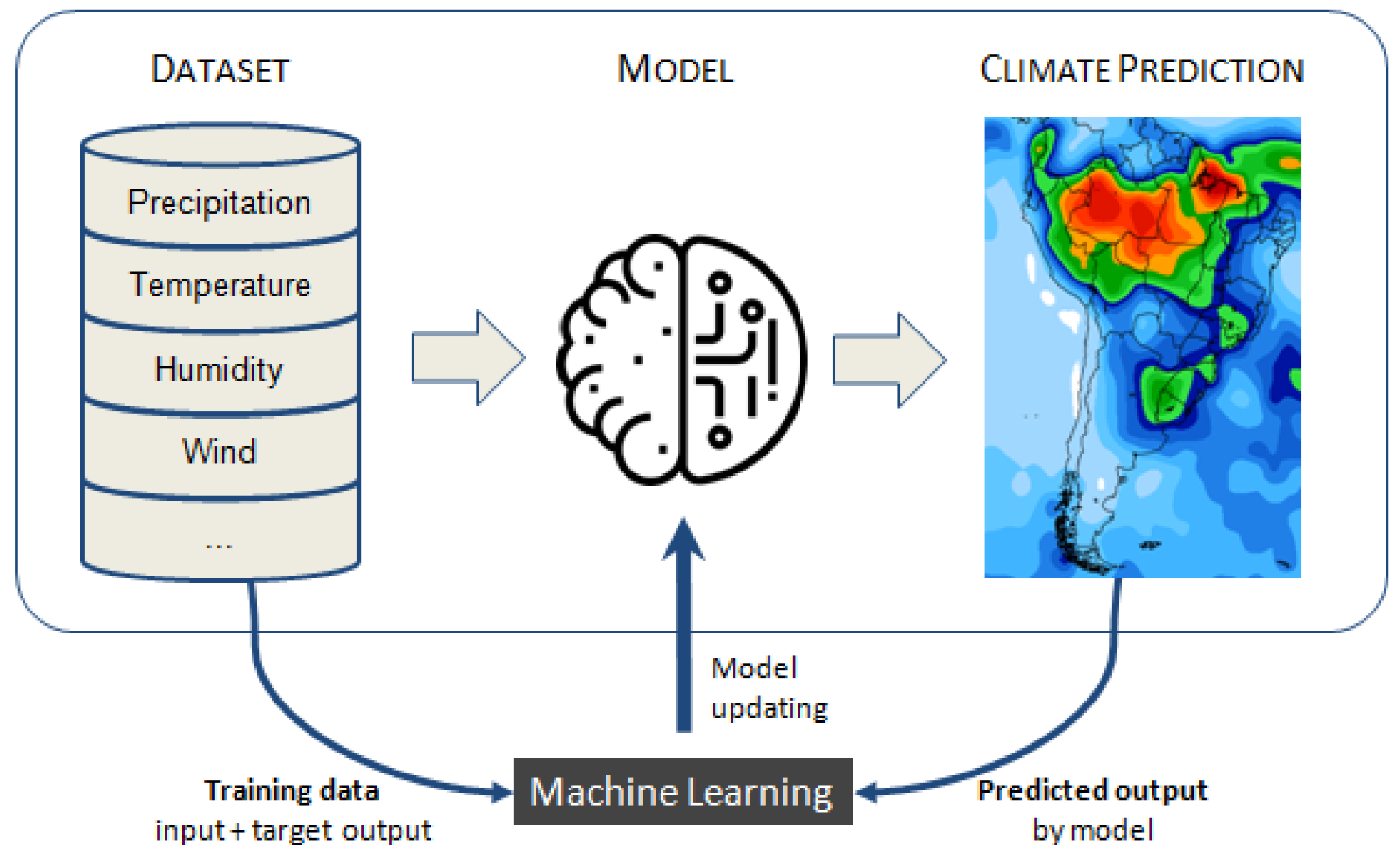
Figure 2 shows the scheme that was implemented in this research. In order to predict future climate conditions, we used a set of meteorological variables as input to produce seasonal climate prediction. These data can be, for example, temperature, wind, and humidity over many years. In this way, a long series of the atmospheric state is created, thus allowing neural network models to estimate future precipitation.
Equation (4) was employed to generate error maps for the analyzed models (multimodel-CPTEC, NN-MPCA, and NN-TensorFlow) for each season.
error map K = { y k d k } ,
where y k is the observation precipitation, and d k is the precipitation calculated by the models at the k-th experimental value at each point of the latitude and longitude coordinates.

4. Results and Discussion

Season-specialist models were developed for precipitation forecasts in South America. In this section, the performance of neural networks developed in TensorFlow (NN-TensorFlow) and MPCA (NN-MPCA) applied to the test dataset (2019) are analyzed in comparison with observation data (GPCP) and an operational model at CPTEC (the BAM model).
As mentioned in Section 2, the training phase is a time-consuming task that involves the search for ideal values of many hyperparameters in order to achieve the optimum topology for the studied problem. After this process a final topology was reached both for NN-TensorFlow and NN-MPCA (Table 1). The function ReLu can be expressed by Equation (5) and the function sigmoid is expressed by Equation (6):
ReLu ( x ) = m a x ( 0 , x )
σ ( x ) = 1 1 + e ( x )
The quantitative prediction performance evaluation metrics for the machine learning models were root-mean-square error (RMSE), covariance (COV), and mean error (ME). Table 2 and Table 3 present the numerical results to evaluate the predictive power of the proposed neural models for the seasonal climate precipitation prediction in the years 2018 and 2019, respectively.
For the year 2018, neural predictors obtained a better prediction performance for all seasons, while the NN-TensorFlow presented the best prediction during the summer, autumn, and winter, and the NN-MPCA showed the best forecasting for the spring—see Table 2. Looking at the evaluation parameters for the year 2019, neural predictors again presented better results. Similar to the year 2018, predictions for the 2019 seasons summer, autumn, and winter were better predicted with NN-TensorFlow, but the NN-MPCA got the best forecast for spring in this year as well—see Table 3.

4.1. Summer Forecast

The summer season in the Southern Hemisphere is characterized by rising temperatures all over the continent, with rapid changes in weather conditions, associated with heavy rain, hail precipitation, moderate to strong winds, and electrical discharges related to deep convection and the development of cumulonimbus clouds with tops reaching over 10 km, mainly in the south, southeast and midwest regions of the country [42].
Figure 3 represents the observed GPCP precipitation field for the summer season, December-January-February (DJF), which is used as a reference in order to compare the performance of the models. The maximum precipitation amounts are located in the north related to the southward displacement of the Intertropical Convergence Zone (ITCZ) and secondary maximums can be found at the southeast and south Brazil, Uruguay, and northeast Argentina. The latter region is often characterized by organized regions of high-top clouds known as the Mesoscale Convective Complex (MCC).
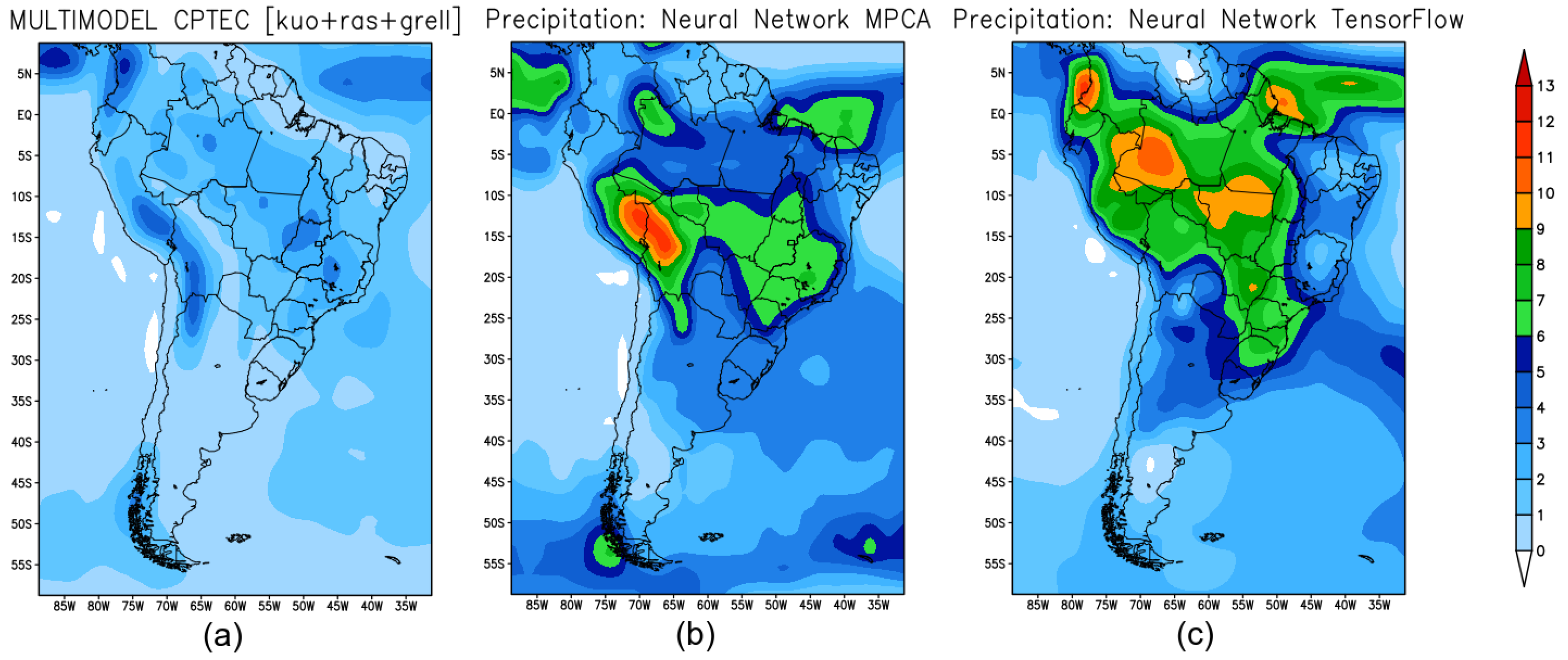
Figure 4 shows the seasonal precipitation prediction for the summer season in 2019 retrieved from forecast models: CPTEC’s BAM model (Figure 4a); NN-MPCA model (Figure 4b); and NN-TensorFlow (Figure 4c). The BAM model is unable to identify precipitation cores in the entire domain. In general, only the NN-TensorFlow is able to resemble the precipitation pattern observed in GPCP (Figure 3). The NN-MPCA model identifies maximums in central and southeast Brazil but is unable to identify high-intensity precipitation in the north related to ITCZ southward displacement, although this model identifies weaker precipitation cores in the ocean close to northeastern Brazil.
Figure 5 shows the error map between the GPCP precipitation dataset and the forecast obtained by the models: Figure 5a is the error map produced for the CPTEC-model; Figure 5b is the error map for NN-MPCA; and Figure 5c is the error map for the NN-TensorFlow model. Analyzing the results of precipitation prediction made by the three models, it is evident that the best result was the NN-TensorFlow (see Figure 4c), where it was able to capture the most intense precipitation patterns, although it overestimated precipitation in the state of Mato Grosso do Sul in Brazil. The results obtained from the NN-MPCA model (see Figure 4b) underestimated precipitation in the entire north region of Brazil and in the Brazilian state Rio Grande do Sul. The CPTEC’s BAM model prediction was unable to capture precipitation patterns; the result for this experiment presented low levels of precipitation over South America.
Analyzing the error map (Figure 5), the CPTEC’s BAM model tends to underestimate the GPCP dataset with values as great as 8 mm in large parts of the northwest and southeast of the continent. The MPCA and TensorFlow also present some underestimation in the Amazon region but with a smaller extent than CPTEC’s BAM model. A great part of the continent presents errors between 0 and 2 mm both for MPCA and TensorFlow but some regions present an overestimation of precipitation, e.g., values up to 6 mm in Mato Grosso do Sul (TensorFlow) and Bolivia (MPCA), among other regions in the equatorial zone.

4.2. Autumn Forecast

The autumn season in the Southern Hemisphere is considered a transition season between summer and winter. During this period, precipitation is more scarce in the interior of Brazil, particularly in the semiarid region of the northeast and in the north of Minas Gerais. In the northern part of the northeast and north regions, it is still a time of heavy rain, especially if the ITCZ persists further south of its climatological position [43].
Figure 6 represents the observed GPCP precipitation field for the autumn season—March-April-May (MAM). The autumn of 2019 had behavior within the average climatology, where significant volumes were observed in the extreme north of South America and there was less precipitation in the other regions, which is characteristic of this autumn season.
Figure 7 shows the seasonal precipitation prediction for the autumn season in 2019 retrieved from forecast models: CPTEC’s BAM model (Figure 7a); NN-MPCA model (Figure 7b); and NN-TensorFlow (Figure 7c). The prediction obtained with the NN-TensorFlow model (Figure 7c) is more similar to the GPCP observation (Figure 6). The NN-MPCA model identified precipitation cores in the Brazilian states: Acre, Amazonia, and northern Pará, southern Colombia and Peru. In the Brazilian states Maranhão, Tocantins, Goias, Mato Grosso, Rondônia, and southern Piaui, the NN-MPCA model overestimated precipitation (see Figure 7b). The BAM model is unable to capture the precipitation observed in GPCP. For this season, the NN-TensorFlow model obtained precipitation patterns similar to GPCP.
Figure 8 shows the error map of the forecast produced from the difference between the GPCP precipitation and the forecast obtained by the models: CPTEC’s BAM model (Figure 8a); NN-MPCA model (Figure 8b); and NN-TensorFlow (Figure 8c). The NN-TensorFlow model presented the least error variation.

4.3. Winter Forecast

The winter season is characterized by lower precipitation amount periods in the southeast, midwest and parts of the north and northeast regions of Brazil, while the largest amounts of precipitation are concentrated in the northwest of the north region, east of the northeast, and part of the southern region of Brazil [44]. This precipitation behavior is highly related to the northward displacement of the ITCZ.
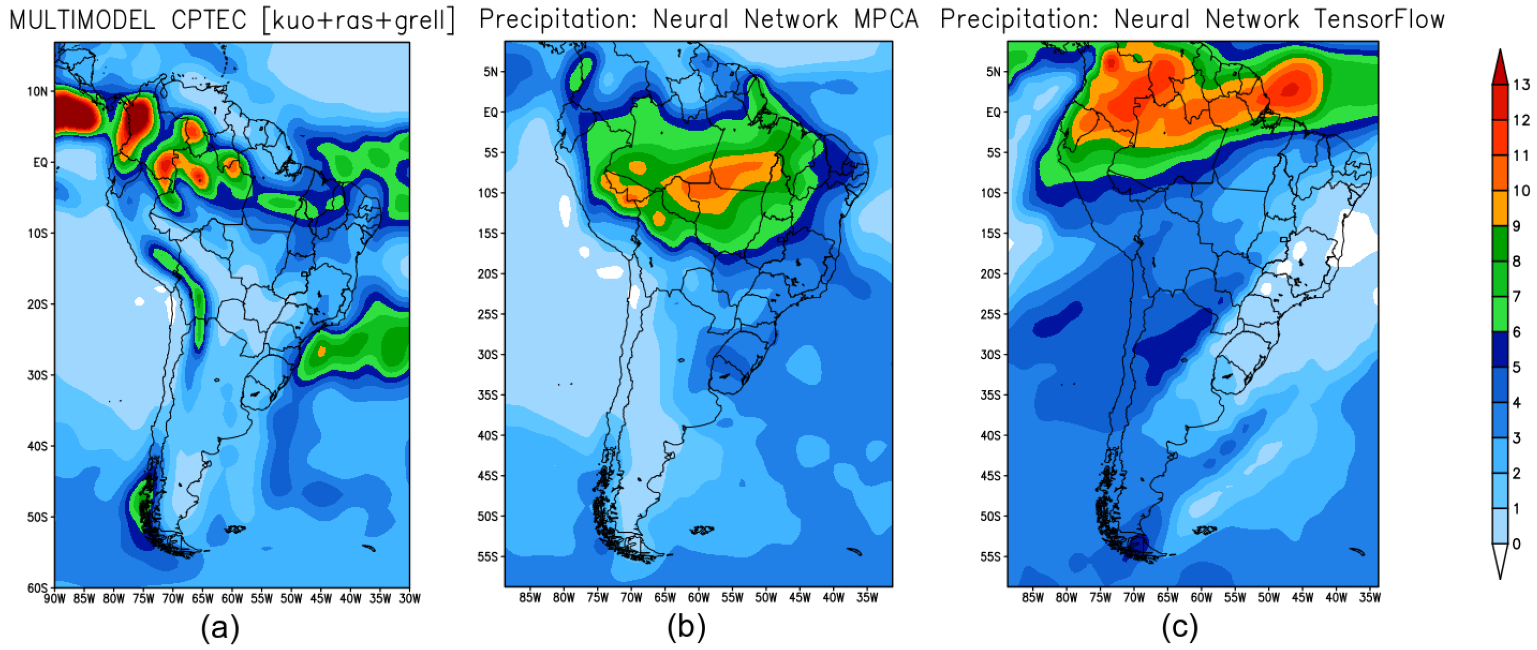
Figure 9 shows the GPCP precipitation for the winter season (June-July-August (JJA)) and Figure 10 shows the seasonal precipitation prediction for the winter season in 2019 retrieved from forecast models: CPTEC’s BAM model (Figure 10a); NN-MPCA model (Figure 10b); and NN-TensorFlow (Figure 10c).
All models are able to identify the precipitation in the extreme north related to the presence of the ITCZ. However, only BAM and NN-TensorFlow have patterns more similar to GCP, whereas MPCA highly overestimates the cores in a larger area and does not identify the oceanic core at the Equatorial Atlantic. In Chile, only BAM and NN-TensorFlow are able to identify the precipitation core shown in GCP. Regarding the south of Brazil, only BAM is able to identify a core related to weather fronts that are characteristic of this region at this time of the year. In the central part of the continent, the westward displacement of the South Atlantic Subtropical High is responsible for low amounts of precipitation.
Figure 11 shows the error map of the forecast models produced from the difference between the GPCP precipitation and the forecast obtained by the models: CPTEC’s BAM model (Figure 11a); NN-MPCA model (Figure 11b); and NN-TensorFlow (Figure 11c). The NN-MPCA error map shows that the model overestimated precipitation in the north and northeast regions of Brazil and Colombia (see Figure 11b). The CPTEC’s BAM model was able to produce the precipitation pattern in central Brazil, and the NN-TensorFlow model was the only one that presented the best forecast result reproducing the precipitation observed in GPCP (see Figure 11c).

4.4. Spring Forecast

The spring season is a transition period between the dry and rainy seasons in central Brazil, as well as the beginning of the convergence of humidity from the Amazon, which defines the quality of the rainy season over the midwest, southeast, and south-central regions, and part of the north region [45].
Figure 12 shows the GPCP precipitation for the spring season (September-October-November (SON)) and Figure 13 shows the seasonal precipitation prediction for the spring season in 2019 retrieved from forecast models: CPTEC’s BAM model (Figure 13a); NN-MPCA model (Figure 13b); and NN-TensorFlow (Figure 13c). The NN-TensorFlow model reproduced the most significant precipitation cores observed in the GPCP data. In the southern region of Brazil, an important region for the agriculture sector, the model reproduced the precipitation pattern very well, as well as in the northern region of Brazil, Colombia, and northern Peru (see Figure 13c).
Figure 14 shows the error map of the forecast models produced from the difference between the GPCP precipitation and the forecast obtained by the models: CPTEC’s BAM model (Figure 14a); NN-MPCA model (Figure 14b); and NN-TensorFlow (Figure 14c). It is notable that the error map produced by the NN-TensorFlow model was the one with the least variation.

4.5. CPU-Time Performance

Models for climate precipitation prediction were executed using different software programming languages and hardware environments. The BAM model was executed on a Cray X50 supercomputer using 120 processing cores: 3 processing nodes, each node with 2 Intel Xeon 2.4 GHz processors with 20 cores per processor. The BAM was codified by the Fortran language with MPI (Message Passing Interface) and OpenMP (Open Multi-Processing) programming patterns for parallel machines. The climate seasonal precipitation prediction with the neural network by the MPCA automatic configuration was codified using a MatLab software environment, using a laptop with an Intel i7 2.4 GHz one-core processor. The deep learning neural network predictor was implemented employing the TensorFlow package under the Python language, and was executed in the Colab Google environment: CPU Intel Xeon 2.2 GHz one-core. All codification was developed using a Linux operating system.
Table 4 shows the CPU time in seconds for each type of model executed on different hardware. As expected, the neural models were much faster than models based on differential equations. The execution of the NN-MPCA in the MatLab environment can be reduced if an executable code is employed.

5. Conclusions

This paper shows the capability of neural networks for seasonal precipitation forecasting over South America. A large dataset from 1980 to 2016 was used for training the season-specialist neural network models and evaluations were performed for the years 2018 and 2019. Additionally, a comparison was performed against the BAM model, an operational state-of-the-art model currently used at the National Institute for Space Research (INPE) in Brazil.
Our results can be summarized as follows:
  • The neural network models are able to resemble the observational patterns throughout the seasons;
  • Larger errors are observed in summer (rainy season on the Continent), and the error magnitude is probably related to high energy availability and local processes that the neural networks are unable to learn due to the spatio-temporal resolution of the training data;
  • Neural networks using TensorFlow have better performance than the ones trained using NN-MPCA for the seasons summer, autumn, and winter, but for the spring season the RMSE was smaller when using the NN-MPCA approach. The latter uses an optimization that takes into account not only the model errors, but also its complexity, looking for the simplest neural network configuration, and such a feature might have affected its ability to learn the precipitation patterns;
  • The comparison to the BAM model showed that neural networks are capable of operational forecasts with better performance, and with a great advantage that there is no need for supercomputers to run these forecasts.
Future works will investigate the use of higher-resolution data for seasonal forecasting in greater resolution.
We also intend to explore the possibility of creating a committee machine between the BAM model and the neural networks as a possibility to simultaneously harness the strengths of both models at operational centers.

Author Contributions

Conceptualization: J.A.A., V.A.d.A. and H.F.d.C.V.; methodology, J.A.A., V.A.d.A. and H.F.d.C.V.; software development: J.A.A. and V.A.d.A.; validation: J.A.A. and V.A.d.A.; writing—original draft preparation: J.A.A., V.A.d.A. and H.F.d.C.V.; writing—review and editing: J.A.A., V.A.d.A. and H.F.d.C.V. All authors have read and agreed to the published version of the manuscript.

Funding

This research received no external funding.

Institutional Review Board Statement

Not applicable.

Informed Consent Statement

Not applicable.

Data Availability Statement

The data are available upon request.

Acknowledgments

Author HFCV wants to thank the National Council for Scientific and Technological Development (CNPq, Brazil) for the research grant number 312924/2017-8. The authors are also grateful for the GPCP precipitation data provided by the NOAA/OAR/ESRL PSL, Boulder, Colorado, USA, from their website at https://psl.noaa.gov/data/gridded/data.gpcp.html accessed on 20 April 2021.

Conflicts of Interest

The authors declare no conflict of interest.

References

  1. Reboita, M.; Gan, M.; Rocha, R.; Ambrizzi, T. Regimes de precipitação na América do Sul: Uma revisão bibliográfica. Rev. Bras. Meteorol. 2010, 25, 185–204. [Google Scholar] [CrossRef]
  2. Krasnopolsky, V.; Fox-Rabinovitz, M.; Belochitski, A. Using Ensemble of Neural Networks to Learn Stochastic Convection Parameterizations for Climate and Numerical Weather Prediction Models from Data Simulated by a Cloud Resolving Model. Adv. Artif. Neural Syst. 2013, 2013, 1–13. [Google Scholar] [CrossRef] [Green Version]
  3. Zanna, L.; Bolton, T. Data-Driven Equation Discovery of Ocean Mesoscale Closures. Geophys. Res. Lett. 2020, 47. [Google Scholar] [CrossRef]
  4. Dijkstra, H.; Petersik, P.; Hernández-García, E.; López, C. The Application of Machine Learning Techniques to Improve El Niño Prediction Skill. Front. Phys. 2019, 7. [Google Scholar] [CrossRef] [Green Version]
  5. Krasnopolsky, V.; Lin, Y. A neural network nonlinear multimodel ensemble to improve precipitation forecasts over continental US. Adv. Meteorol. 2012, 2012. [Google Scholar] [CrossRef]
  6. NOAA Artificial Intelligence Strategy: Analytics for Next-Generation Earth Science. Available online: https://nrc.noaa.gov/ (accessed on 20 February 2021).
  7. AI and Machine Learning at ECMWF. Available online: https://www.ecmwf.int/en/newsletter/163/news/ai-and-machine-learning-ecmwf/ (accessed on 20 February 2021).
  8. Bouttier, F.; Marchal, H. Probabilistic thunderstorm forecasting by blending multiple ensembles. Tellus Ser. A Dyn. Meteorol. Oceanogr. 2020, 72, 1–19. [Google Scholar] [CrossRef] [Green Version]
  9. Kosaka, Y.; Chowdary, J.S.; Xie, S.P.; Min, Y.M.; Lee, J.Y. Limitations of Seasonal Predictability for Summer Climate over East Asia and the Northwestern Pacific. J. Clim. 2012, 25, 7574–7589. [Google Scholar] [CrossRef]
  10. Mariotti, A.; Ruti, P.M.; Rixen, M. Progress in subseasonal to seasonal prediction through a joint weather and climate community effort. NPJ Clim. Atmos. Sci. 2018, 1. [Google Scholar] [CrossRef]
  11. Weisheimer, A.; Palmer, T.N. On the reliability of seasonal climate forecasts. J. R. Soc. Interface 2014, 11. [Google Scholar] [CrossRef] [PubMed]
  12. Robertson, A.W.; Vitart, F.; Camargo, S.J. Subseasonal to seasonal prediction of weather to climate with application to tropical cyclones. J. Geophys. Res. Atmos. 2020, 125, e2018JD02937. [Google Scholar] [CrossRef]
  13. Anochi, J.; Hernández Torres, R.; Campos Velho, H. Two Geoscience Applications by Optimal Neural Network Architecture. Pure Appl. Geophys. 2020, 177, 2663–2683. [Google Scholar] [CrossRef]
  14. Anochi, J.; Campos Velho, H. Optimization of feedforward neural network by Multiple Particle Collision Algorithm. In Proceedings of the 2014 IEEE Symposium on Foundations of Computational Intelligence (FOCI), Orlando, FL, USA, 9–12 December 2014; pp. 128–134. [Google Scholar]
  15. Anochi, J. Previsão Climática De Precipitação Por Redes Neurais Autoconfiguradas. Ph.D. Thesis, Instituto Nacional de Pesquisas Espaciais, São José dos Campos, Brazil, 2015. [Google Scholar]
  16. Benardos, P.; Vosniakos, G. Optimizing feedforward artificial neural network architecture. Eng. Appl. Artif. Intell. 2007, 20, 365–382. [Google Scholar] [CrossRef]
  17. Carvalho, A.; Ramos, F.; Chaves, A. Metaheuristics for the feedforward artificial neural network (ANN) architecture optimization problem. Neural Comput. Appl. 2011, 20, 1273–1284. [Google Scholar] [CrossRef] [Green Version]
  18. Litzinger, S.; Klos, A.; Schiffmann, W. Compute-Efficient Neural Network Architecture Optimization by a Genetic Algorithm. In Proceedings of the Lecture Notes in Computer Science (Including subseries Lecture Notes in Artificial Intelligence and Lecture Notes in Bioinformatics), Munich, Germany, 17–19 September 2019; pp. 387–392. [Google Scholar]
  19. Echevarría, L.; Santiago, O.; Silva Neto, A. Aplicación de los algoritmos evolución diferencial y colisión de partículas al diagnóstico de fallos en sistemas industriales. Investig. Oper. 2012, 33, 160–172. [Google Scholar]
  20. Sambatti, S.; Anochi, J.; Luz, E.; Carvalho, A.; Shiguemori, E.; Campos Velho, H. Automatic configuration for neural network applied to atmospheric temperature profile identification. In Proceedings of the 3rd International Conference on International Conference on Engineering Optimization, Rio de Janeiro, Brazil, 1–5 July 2012. [Google Scholar]
  21. Hernández Torres, R.; Campos Velho, H.; Chiwiacowsky, L. Rotation-based multi-particle collision algorithm with Hooke-Jeeves approach applied to the structural damage identification. In Computational Intelligence, Optimization and Inverse Problems with Applications in Engineering; Springer: Cham, Switzerland, 2018; pp. 87–109. [Google Scholar]
  22. Hernández Torres, R.; Luz, E.; Campos Velho, H. Multi-Particle Collision Algorithm for Solving an Inverse Radiative Problem. In Integral Methods in Science and Engineering; Birkhauser: Cham, Seitzerland, 2015; pp. 309–319. [Google Scholar]
  23. Penha Neto, G.; Campos Velho, H.; Shiguemori, E. UAV autonomous navigation by image processing with uncertainty trajectory estimation. In Proceedings of the International Symposium on Uncertainty Quantification and Stochastic Modeling, Rouen, France, 29 June–3 July 2021; pp. 211–221. [Google Scholar]
  24. Anochi, J.; Hernández Torres, R.; Campos Velho, H. Climate precipitation prediction with uncertainty quantification by self-configuring neural network. In Proceedings of the International Symposium on Uncertainty Quantification and Stochastic Modeling, Rouen, France, 29 June–3 July 2021; pp. 242–253. [Google Scholar]
  25. Cintra, R.; Campos Velho, H.; Anochi, J.; Cocke, S. Data assimilation by artificial neural networks for the global FSU atmospheric model: Surface pressure. In Proceedings of the 2015 Latin-America Congress on Computational Intelligence, LA-CCI 2015, Curitiba, Brazil, 13–16 October 2016. [Google Scholar]
  26. Sacco, W.; Oliveira, C. A new stochastic optimization algorithm based on particle collisions. Trans. Am. Nucl. Soc. 2005, 92, 657–659. [Google Scholar]
  27. Sacco, W.; Oliveira, C.; Pereira, C. Two stochastic optimization algorithms applied to nuclear reactor core design. Prog. Nucl. Energy 2006, 48, 525–539. [Google Scholar] [CrossRef]
  28. Sacco, W.; Filho, H.; Pereira, C. Cost-Based Optimization of a Nuclear Reactor Core Design: A Preliminary Model; 2007; pp. 1–6. Available online: https://inis.iaea.org/search/searchsinglerecord.aspx?recordsFor=SingleRecord&RN=39107793 (accessed on 20 April 2021).
  29. Sacco, W.; Lapa, C.; Pereira, C.; Alves Filho, H. A Metropolis Algorithm applied to a Nuclear Power Plant Auxiliary Feedwater System surveillance tests policy optimization. Prog. Nucl. Energy 2008, 50, 15–21. [Google Scholar] [CrossRef]
  30. Kirkpatrick, S.; Gelatt, C.; Vecchi, M. Optimization by simulated annealing. Science 1983, 220, 671–680. [Google Scholar] [CrossRef]
  31. Luz, F.; Becceneri, J.; Campos Velho, H. A new multi-particle collision algorithm for optimization in a high performance environment. J. Comput. Interdiscip. Sci. 2008, 1, 3–10. [Google Scholar] [CrossRef] [Green Version]
  32. Luz, E.; Becceneri, J.; Campos Velho, H. Multiple Particle Collision Algorithm applied to radiative transference and pollutant localization inverse problems. In Proceedings of the IEEE International Symposium on Parallel and Distributed Processing Workshops and Phd Forum, Anchorage, AK, USA, 16–20 May 2011; pp. 347–351. [Google Scholar]
  33. Abadi, M.; Agarwal, A.; Barham, P.; Brevdo, E.; Chen, Z.; Citro, C.; Corrado, G.; Davis, A.; Dean, J.; Devin, M.; et al. TensorFlow: Large-Scale Machine Learning on Heterogeneous Distributed Systems. arXiv 2016, arXiv:1603.04467. [Google Scholar]
  34. Adler, R.F.; Huffman, G.J.; Chang, A.; Ferraro, R.; Xie, P.P.; Janowiak, J.; Rudolf, B.; Schneider, U.; Curtis, S.; Bolvin, D.; et al. The version-2 global precipitation climatology project (GPCP) monthly precipitation analysis (1979-present). J. Hydrometeorol. 2003, 4, 1147–1167. [Google Scholar] [CrossRef]
  35. Kalnay, E.; Kanamitsu, M.; Kistler, R.; Collins, W.; Deaven, D.; Gandin, L.; Iredell, M.; Saha, S.; White, G.; Woollen, J.; et al. The NCEP/NCAR 40-year reanalysis project. Bull. Am. Meteorol. Soc. 1996, 77, 437–472. [Google Scholar] [CrossRef] [Green Version]
  36. Figueroa, S.N.; Bonatti, J.P.; Kubota, P.Y.; Grell, G.A.; Morrison, H.; Barros, S.R.; Fernandez, J.P.; Ramirez, E.; Siqueira, L.; Luzia, G.; et al. The Brazilian Global Atmospheric Model (BAM): Performance for tropical rainfall forecasting and sensitivity to convective scheme and horizontal resolution. Weather. Forecast. 2016, 31, 1547–1572. [Google Scholar] [CrossRef]
  37. Kubota, P. Variability of Storage Energy in the Soil-Canopy System and Its Impact on the Definition of Precipitation Standard in South America. Ph.D. Thesis, Instituto Nacional de Pesquisas Espaciais, São José dos Campos, Brazil, 2012. [Google Scholar]
  38. Morrison, H.; Curry, J.; Khvorostyanov, V. A new double-moment microphysics parameterization for application in cloud and climate models. Part I: Description. J. Atmos. Sci. 2005, 62, 1665–1677. [Google Scholar] [CrossRef]
  39. Morrison, H.; Thompson, G.; Tatarskii, V. Impact of cloud microphysics on the development of trailing stratiform precipitation in a simulated squall line: Comparison of one- and two-moment schemes. Mon. Weather. Rev. 2009, 137, 991–1007. [Google Scholar] [CrossRef] [Green Version]
  40. Iacono, M.; Delamere, J.; Mlawer, E.; Shephard, M.; Clough, S.; Collins, W. Radiative forcing by long-lived greenhouse gases: Calculations with the AER radiative transfer models. J. Geophys. Res. Atmos. 2008, 113. [Google Scholar] [CrossRef]
  41. Park, S.; Bretherton, C.S. The University of Washington shallow convection and moist turbulence schemes and their impact on climate simulations with the community atmosphere model. J. Clim. 2009, 22, 3449–3469. [Google Scholar] [CrossRef]
  42. Prognóstico Climático de Verão. Available online: https://portal.inmet.gov.br/notasTecnicas# (accessed on 12 January 2021).
  43. Prognóstico Climático de Outono. Available online: https://portal.inmet.gov.br/notasTecnicas# (accessed on 12 January 2021).
  44. Prognóstico Climático de Inverno. Available online: https://portal.inmet.gov.br/notasTecnicas# (accessed on 12 January 2021).
  45. Prognóstico Climático de Primavera. Available online: https://portal.inmet.gov.br/notasTecnicas# (accessed on 12 January 2021).
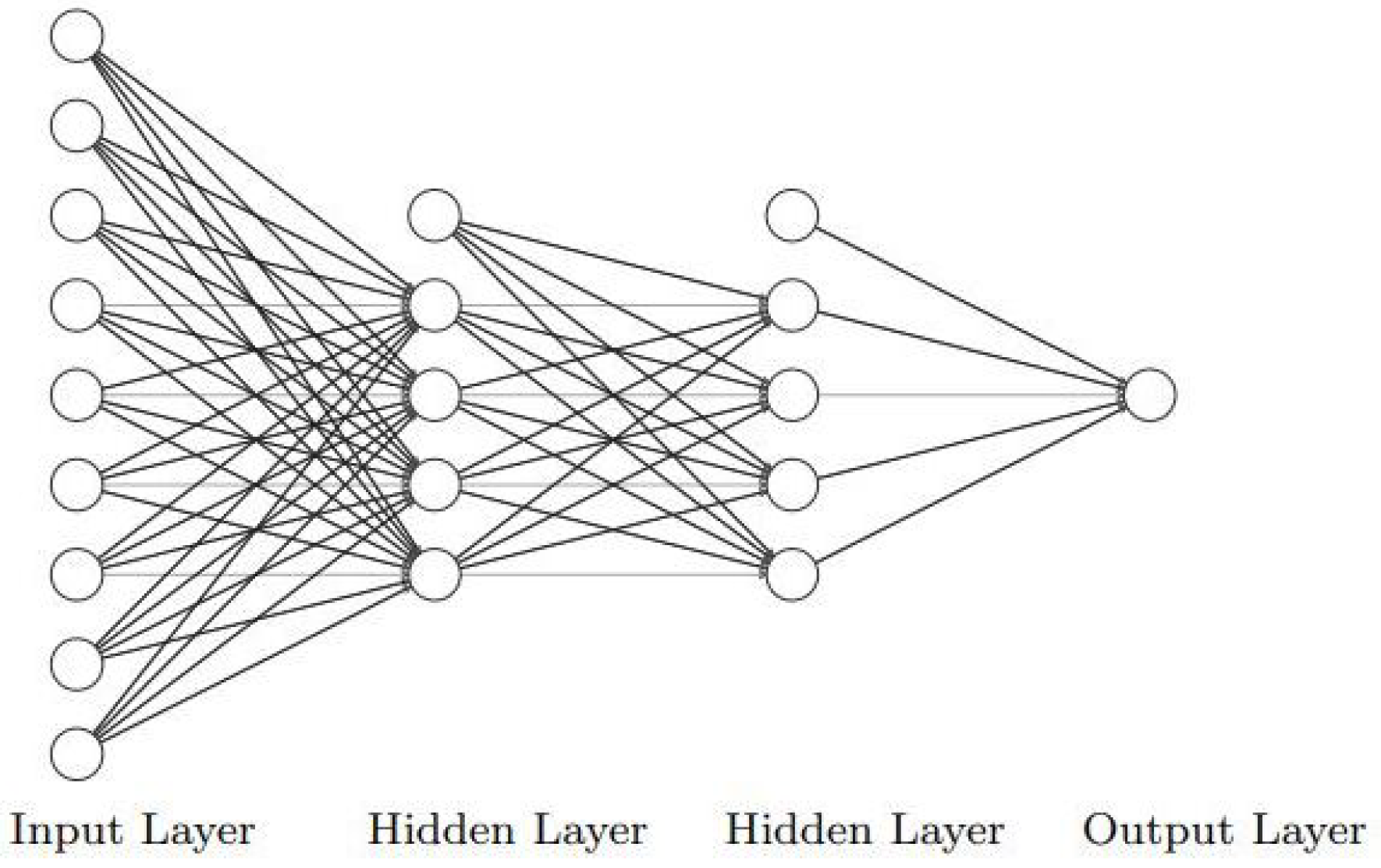
Figure 1. Typical topology of a neural network.
Remotesensing 13 02468 g001
Figure 2. Schematic representation of prediction methodology.
Remotesensing 13 02468 g002
Figure 3. GPCP precipitation—summer 2019.
Remotesensing 13 02468 g003
Figure 4. Seasonal climate prediction for the summer over South America: (a) precipitation predicted by CPTEC’s BAM model; (b) prediction by NN-MPCA; (c) precipitation prediction by NN-TensorFlow.
Remotesensing 13 02468 g004
Figure 5. Error map to evaluate the performance of the forecast models: (a) CPTEC’s BAM model; (b) NN-MPCA; and (c) NN-TensorFlow.
Remotesensing 13 02468 g005
Figure 6. GPCP precipitation—autumn 2019.
Remotesensing 13 02468 g006
Figure 7. Seasonal climate prediction for the autumn in South America: (a) precipitation predicted by CPTEC’s BAM model; (b) prediction obtained by NN-MPCA; (c) precipitation prediction obtained by using the NN-TensorFlow.
Remotesensing 13 02468 g007
Figure 8. Error map for the autumn in South America to evaluate the performance of the forecast models: (a) CPTEC’s BAM model; (b) NN-MPCA; and (c) NN-TensorFlow.
Remotesensing 13 02468 g008
Figure 9. GPCP precipitation—winter 2019.
Remotesensing 13 02468 g009
Figure 10. Seasonal climate prediction for the winter in South America: (a) precipitation predicted by CPTEC’s BAM model; (b) prediction obtained by NN-MPCA; (c) precipitation prediction obtained using the NN-TensorFlow.
Remotesensing 13 02468 g010
Figure 11. Error map for the winter in South America to evaluate the performance of the forecast models: (a) CPTEC’s BAM model; (b) NN-MPCA; and (c) NN-TensorFlow.
Remotesensing 13 02468 g011
Figure 12. GPCP precipitation—spring 2019.
Remotesensing 13 02468 g012
Figure 13. Seasonal climate forecast for the spring in South America: (a) precipitation predicted by CPTEC’s BAM model; (b) prediction obtained by NN-MPCA; (c) prediction obtained by NN-TensorFlow.
Remotesensing 13 02468 g013
Figure 14. Error map for the spring in South America to evaluate the performance of the forecast models: (a) error map produced from the difference between the GPCP precipitation dataset and the precipitation prediction by Multimodel-CPTEC; (b) error map for the NN-MPCA; and (c) error map for the NN-TensorFlow.
Remotesensing 13 02468 g014
Table 1. Final topology and other characteristics of neural networks in TensorFlow and MPCA experiments.
ParametersNN-TensorFlowNN-MPCA
Version2.0.01.0
Number of inputs99
Number of layers21
Number of hidden neurons (each layer)2520
Activation function (hidden layers)ReLUsigmoid logistic
Activation function (output)linearsigmoid logistic
OptimizerAdam 1backpropagation
Learning rate0.001 (default)0.2
Momentum0.9 (default)0.4
Epochs10001000
1https://keras.io/api/optimizers/adam/, accessed on 20 March 2021.
Table 2. Prediction performance measures in 2018.
Season/MethodsBAMNN-MPCANN-TensorFlow
RMSECOVMERMSECOVMERMSECOVME
Summer13.767.772.447.987.67−0.557.638.61−0.12
Autumn12.495.852.575.894.751.060.860.85−0.07
Winter9.544.341.7820.8318.50−1.528.968.56−1.18
Spring8.633.862.183.111.591.234.203.27−0.96
Table 3. Prediction performance measures in 2019.
Season/MethodsBAMNN-MPCANN-TensorFlow
RMSECOVMERMSECOVMERMSECOVME
Summer11.856.802.244.934.800.362.512.500.09
Autumn6.306.230.285.064.440.781.401.40−0.02
Winter4.784.60−0.4117.6616.331.151.321.20−0.34
Spring3.813.72−0.292.581.661.255.273.691.25
Table 4. CPU time in seconds for the prediction execution for different models.
Models
Hardware
BAM
Cray X50 120-cores
NN-MPCA
Laptop Intel 1-core
NN-TensorFlow
Colab Intel 1-core
CPU time 9.60 × 10 3  s22.19 s0.15 s
Publisher’s Note: MDPI stays neutral with regard to jurisdictional claims in published maps and institutional affiliations.