Abstract
The emergence of the spectral variation hypothesis (SVH) has gained widespread attention in the remote sensing community as a method for deriving biodiversity information from remotely sensed data. SVH states that spectral heterogeneity on remotely sensed imagery reflects environmental heterogeneity, which in turn is associated with high species diversity and, therefore, could be useful for characterizing landscape biodiversity. However, the effect of phenology has received relatively less attention despite being an important variable influencing plant species spectral responses. The study investigated (i) the effect of phenology on the relationship between spectral heterogeneity and plant species diversity and (ii) explored spectral angle mapper (SAM), the coefficient of variation (CV) and their interaction effect in estimating species diversity. Stratified random sampling was adopted to survey all tree species with a diameter at breast height of > 10 cm in 90 × 90 m plots distributed throughout the study site. Tree species diversity was quantified by the Shannon diversity index (H′), Simpson index of diversity (D2) and species richness (S). SAM and CV were employed on Landsat-8 data to compute spectral heterogeneity. The study applied linear regression models to investigate the relationship between spectral heterogeneity metrics and species diversity indices across four phenological stages. The results showed that the end of the growing season was the most ideal phenological stage for estimating species diversity, following the SVH concept. During this period, SAM and species diversity indices (S, H′, D2) had an r2 of 0.14, 0.24, and 0.20, respectively, while CV had an r2 of 0.22, 0.22, and 0.25, respectively. The interaction of SAM and CV improved the relationship between the spectral data and H′ and D2 (from r2 of 0.24 and 0.25 to r2 of 0.32 and 0.28, respectively) at the end of the growing season. The two spectral heterogeneity metrics showed differential sensitivity to components of plant diversity. SAM had a high relationship with H′ followed by D2 and then a lower relationship with S throughout the different phenological stages. Meanwhile, CV had a higher relationship with D2 than other plant diversity indices and its relationship with S and H′ remained similar. Although the coefficient of determination was comparatively low, the relationship between spectral heterogeneity metrics and species diversity indices was statistically significant (p < 0.05) and this supports the assertion that SVH could be implemented to characterize plant species diversity. Importantly, the application of SVH should consider (i) the choice of spectral heterogeneity metric in line with the purpose of the SVH application since these metrics relate to components of species diversity differently and (ii) vegetation phenology, which affects the relationship that spectral heterogeneity has with plant species diversity.
1. Introduction
Remote sensing application in biodiversity research has long been a topical subject. The subject focused mostly on the utility of remotely sensed data for identifying biodiversity hotspots, assessing species richness and distributions and modeling biodiversity responses to changing environmental conditions [1] (Turner et al., 2003). The interest in remote sensing originated from the realization that efforts toward successful biodiversity conservation necessitate frequent and detailed spatial information on species richness and distribution and their habitat conditions [1,2] (Turner et al., 2003; Kerr and Ostrovsky, 2003). Remote sensing satellites repeatedly collect data over large geographic areas at varying levels of spatial resolutions. Therefore, remote sensing satellites have two advantages over traditional field surveys: (i) the repeated collection allows for regular assessments of temporal changes in biodiversity and (ii) the availability of data in different spatial resolutions facilitates the multi-scale assessment of biodiversity [3,4]. These features of satellite remote sensing make it an attractive source of data for biodiversity studies.
One particular study characterized two approaches often adopted when applying remote sensing in biodiversity studies [1] (Turner et al., 2003). The first approach is the direct remote sensing of species and species assemblages and the second approach is the indirect estimation of species diversity by using remotely sensed environmental parameters. The former involves primarily the classification of a remotely sensed image into species classes, which has been criticized for degrading continuous, measurable information into isolated classes [5] (Palmer et al., 2002). Meanwhile, indirect remote sensing approaches entails using surrogate variables, such as the normalized difference vegetation index (NDVI) and its derivatives, for estimating biodiversity [6,7,8,9,10] (Fairbanks and McGwire, 2004; Gould, 2000; He et al., 2009; Oindo and Skidmore, 2002; Parviainen et al., 2010). The basis of indirect application emanates from ecological theories explaining biodiversity. For instance, the use of NDVI emanates from the observation that it is related to ecosystem primary productivity, which explains the spatial variation in species diversity [10,11] (Parviainen et al., 2010; Witman et al., 2008). This NDVI-primary productivity nexus saw NDVI being used for estimating species diversity in various ecosystems [9,10,12,13] (Oindo and Skidmore, 2002; Parviainen et al., 2010; Pau et al., 2012; Madonsela et al., 2018).
Consistent with the aforementioned second approach, Palmer et al., (2002) [5] proposed a spectral variation hypothesis (SVH) as a method for deriving biodiversity information from remotely sensed data. The SVH follows the ecological argument that environmental heterogeneity supports high species diversity in that greater environmental gradient, resource, and structural complexity increase the number of available niches and thus, allow more species to coexist [14] (Stein et al., 2014). In this regard, SVH states that spectral heterogeneity on remotely sensed image reflects the spatial variation in the environment, which in turn is associated with species richness [5] (Palmer et al., 2002). Subsequently, spectral heterogeneity on a remotely sensed image was put forward as a spectral indicator of plant species diversity [5,15,16] (Palmer et al., 2002; Rocchini et al., 2010; Féret and Asner, 2014).
As such, studies have tested SVH in several ecosystems, using various spectral heterogeneity metrics, and observed varying levels of relationships between spectral heterogeneity and species diversity (see compilation listed in Schmidtlein and Fassnacht (2017)) [17]. A large proportion of these studies achieved correlation or a coefficient of determination of 30–85%, while others achieved less than 20%. Despite this variation in the relationship between spectral heterogeneity and species diversity, there is a growing consensus that spectral heterogeneity on a remotely sensed image can provide a sensible assessment of plant species diversity [3,4,18] (Warren et al., 2014; Rocchini et al., 2016; Schweiger et al., 2018). However, Schmidtlein and Fassnacht (2017) [17] questioned the general applicability of SVH following the observation that high spectral heterogeneity does not always correspond to high species richness and vice versa. Schmidtlein and Fassnacht (2017) [17] noted that unevenness within the floristic mapping units creates a robust gradient in spectral heterogeneity and this gradient does not always relate to the species richness gradient. In fact, their study concluded that SVH is ecosystem dependent, following their observation of the inconsistent association between spectral heterogeneity and species diversity in southern Germany.
Moreover, Oldeland et al. (2010) [19] also observed high spectral heterogeneity not related to species diversity in one sample collected in the commercial game farming site, due to the heterogeneity of the savannah landscape. Savannahs, in general, are characterized by the co-occurrence of a continuous layer of grass and patchy woody vegetation with pockets of bare areas [20] (Scholes and Archer, 1997), and this heterogeneity in the savannah landscape had a negative influence on the pooled regression analysis performed by Oldeland et al. (2010) [19]. However, increasing the window of analysis improved model fitting in Oldeland et al. (2010) [19] and this trend further stressed the assertion in the literature that the relationship between spectral heterogeneity and species diversity is scale-dependent [5,21,22] (Palmer et al., 2002; Rocchini et al., 2004; González-Megías et al., 2007).
While the emergence of SVH has gained widespread attention in the remote sensing community as a method for deriving biodiversity information from remotely sensed data [3,15,18,19,21,22,23] (Oldeland et al., 2010; González-Megías et al., 2007; Rocchini et al., 2004; Rocchini, 2007; Rocchini et al., 2010; Schweiger et al., 2018; Warren et al., 2014), the effect of phenology has received relatively less attention with few studies considering it [17] (Schmidtlein and Fassnacht, 2017) despite being an essential variable influencing plant species’ spectral behavior. Compared to the scale issue, which has shown that its increase could impact positively or negatively on SVH [17,19,21] (Schmidtlein and Fassnacht, 2017; Oldeland et al., 2010; Rocchini et al., 2004), little is known about the impact of phenology on the relationship between spectral heterogeneity and species diversity, especially in the savannah ecosystem. In an experiment in prairie grasslands, Gholizadeh et al. (2020) [24] observed that a shift in phenology affected the relationship between spectral heterogeneity metrics and species richness and that the relationship between spectral heterogeneity metrics and species richness may change between years, regardless of the phenology. However, it must be noted that the experiment was conducted in an ecosystem where (i) a shift in phenology was accompanied by a change in species richness and (ii) there was prescribed burning, which might have affected the spectral reflectance, as it alters the percentage cover of individual species and the background characteristics of the landscape [24,25] (Flanagan et al., 2015; Gholizadeh et al., 2020). In an alpine coniferous forest, Torresani et al. (2019) observed that the relationship between spectral heterogeneity and tree species diversity was highest during the summer period when the NDVI reached its peak and lowest during the winter period. This observation contradicts that of Hill et al. (2010) [26], who observed that the optimal period for mapping forest classes is at the beginning or the end of the growing season when plants are at different phenological stages, rather than mid-summer in a temperate forest. Meanwhile, Lopes et al. (2017) [27] observed that multi-temporal data do not enhance the relationship between spectral heterogeneity and the Shannon diversity index in a grassland experimental site, southwest of France. This observation was attributed to management decisions, such as mowing, grazing and fertilizing, which may have impacted the grasslands phenological and spectral behavior.
Conceptually, phenological variations between plant species should enhance their spectral differences, thus increasing the spectral heterogeneity in the image. This takes place when plant species are at different phenological stages in one image as a result of differential phenological changes between plant species [26,28,29] (Gilmore et al., 2008; Hill et al., 2010; Madonsela et al., 2017). With this understanding, it is reasonable to assume that at an optimal phenological stage when plant species are at their different phenological stages, the relationship between spectral heterogeneity and species diversity could be enhanced. This assumption has not been tested in the savannah ecosystem and the present study examines the relationship between tree species diversity and Landsat-8 spectral heterogeneity across multiple phenological stages in the savannah woodland in order to define the most ideal phenological stage for estimating species diversity, using remotely sensed data. This study builds on the work of Oldeland et al. (2010) [19], who tested the SVH in the African savannah and observed promising results between the Shannon diversity index and spectral heterogeneity. Other studies [17,24,30,31] (Schmidtlein and Fassnacht, 2017; Wang et al., 2018; Torresani et al., 2019; Gholizadeh et al., 2020), however, were conducted in different ecosystems.
In testing the SVH theory, studies experimented with different spectral heterogeneity metrics and different measures of plant diversity, which affected the conclusions drawn in these studies regarding SVH. For instance, Oldeland et al. (2010) [19] and Wang et al. (2018) applied the mean of the Euclidean distances from the centroid and coefficient of variation (CV), respectively, and concluded that abundance-based measures of plant diversity related better with the spectral data than species richness. Meanwhile, Torresani et al. (2019) [30] applied the Rao’s Q index and CV against the Shannon diversity index and concluded that Rao’s Q index was more suited to characterize plant diversity than CV. These conclusions are partial, given that, in the case of Oldeland et al. (2010) [19] and Wang et al. (2018) [31], only one spectral heterogeneity metric was applied, while in the case of Torresani et al. (2019) [30], the two spectral heterogeneity metrics were tested against the Shannon diversity index only. It is important to notice that (i) spectral heterogeneity metrics characterize spectral heterogeneity differently [32] (Gholizadeh et al., 2018) and (ii) the measures of plant diversity also consider different properties of plant communities in varying ways when quantifying species diversity [33,34] (Morris et al., 2014; Nagendra et al., 2002). Therefore, there is a need for further inquiry into the relationship between spectral heterogeneity and species diversity while exploring the temporal behavior of spectral heterogeneity metrics in relation to the components of the plant communities considered, i.e., richness and abundance. Incorporating phenology could shed some light in understanding the spectral heterogeneity described by spectral heterogeneity metrics. This study contributes to the advancement of the SVH, as it (i) investigates the effect of phenology on the relationship between spectral heterogeneity and species diversity, (ii) explores Spectral Angle Mapper (SAM), CV and their interaction effect in estimating species diversity and (iii) describes the sensitivity of spectral heterogeneity metrics to components of plant communities.
2. Study Site
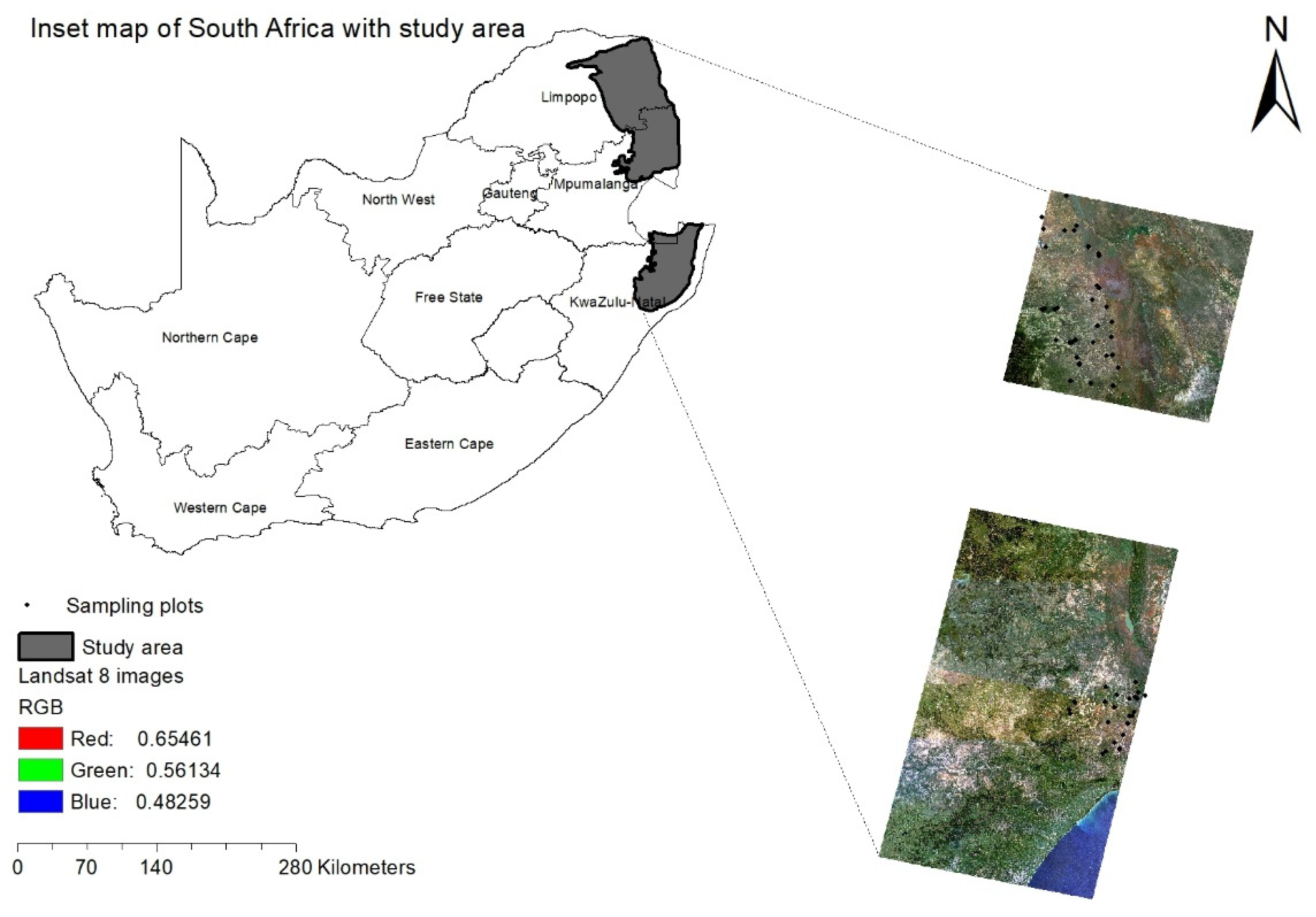
The study site extends over the savannah woodland, covering three provinces, i.e., Mpumalanga, Limpopo and KwaZulu-Natal (KZN) of South Africa (Figure 1). Our study site is managed differently across space with one part sitting in protected landscapes in Kruger National Park (KNP) and Hluhluwe-Imfolozi Park and the other part sitting in communal areas under traditional authority. Consistent with savannah settings, the study area is characterized by the continuous grassy vegetation interspersed with sparsely distributed tree layers [20,35] (Scholes and Archer, 1997; Sankaran et al., 2005). These two lifeforms often remain in a balanced distributional pattern in the presence of fires, rainfall and herbivory, which are the primary controlling variables [35,36] (Sankaran et al., 2005; Bond et al., 2003).
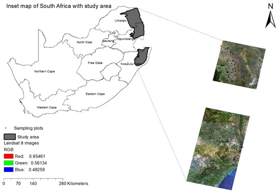
Figure 1.
Area under study extending over the savannah ecosystem of South Africa with Landsat-8 image. The dots denote the field plots.
In terms of physical structure, granite geological formations occur dominantly in the western part, while the eastern part is occupied by gabbro substrate. Dark clay soils characterize the gabbro substrate, which supports nutritious grasses with few dispersed trees, typically Acacia spp. [37] (Scogings, 2004). Meanwhile, the granite substrate is characterized by deep sand soils with poor nutrient content, which supports deciduous tree species. Moreover, high species diversity were observed on the granite substrates [37,38] (Scogings, 2004; Eckhardt et al., 2000). The study site is also occupied largely by Colophospermum mopane in the northern part [38,39] (Eckhardt et al., 2000; Makhado et al., 2014). The average annual rainfall ranges from 440 mm in the northern part of Kruger National Park to 750 mm in the south with noticeable deviations around the average over time [38,39] (Makhado et al., 2014; Eckhardt et al., 2000).
3. Materials and Methods
3.1. Remotely Sensed Data
The study used four images collected by Landsat-8 Operational Land Imager (OLI) and these images were acquired freely from the USGS download portal. Landsat-8 sensor has eight spectral bands covering the visible, near-infrared (NIR) and shortwave infrared (SWIR) regions. The sensor collects data at a coarse spatial resolution of 30 m and has a temporal resolution of 16 days. The enhanced signal-to-noise ratio of the Landsat-8 sensor, together with its 12-bit quantization of data, makes it more useful for land cover mapping [40] (Pervaiz et al., 2016). The four images were acquired in 2016 (28 March, 29 April, 31 May, and 24 July), covering four phenological stages. These dates correspond to the end of the growing season [41] (Grant and Scholes, 2006), the transition to senescence [29] (Madonsela et al., 2017), the advanced senescence stage when most trees start to defoliate [42,43] (Scholes and Eckhardt, 2003; Cho et al., 2010) and the dry season in the southern African savannah [37,44] (Scogings, 2004; Kaszta et al., 2016), respectively.
The images were corrected for atmospheric distortions, using ATCOR software. ATCOR-2 was applied to images covering Mpumalanga and Limpopo for processing atmospheric distortions. Meanwhile, the KZN images were corrected atmospherically, using ATCOR-3 since the area is mountainous [45] (Ritcher and Schläpfer, 2005). In addition, WorldView-2 scene—collected over a tiny portion of the study site—was acquired on the 7 March 2013 within the savannah woodland (for more details see [29] Madonsela et al., 2017). The WV-2 image was only used in the design of sampling plots.
3.2. Field Campaign and Data Collection
The study launched two field excursions in November 2015 and March 2016 in KwaZulu-Natal and across KNP extending between Mpumalanga and Limpopo. Initially, the study defined the size of field plots, using semi-variogram analysis in ENVI 4.8 software. A semi-variogram computes the diversity of the natural phenomenon that occurs over space [46,47]. A semi-variogram is calculated as follows:
where y(h) represents the semi-variance at a given distance h; z(xi) is the value of the variable Z at location xi; h is the lag distance; and N (h) is the number of pairs of sample points separated by h.
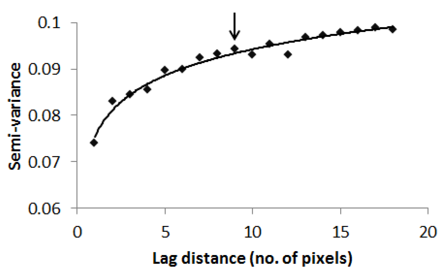
Semi-variance steadily upsurges as the distance from one point to subsequent point widens until it gets to the range where it begins to flatten out [46,48] (Jongman and Jongman, 1995; Grignaten and Deutsch, 2001). In this study, the semi-variogram technique was applied to a 10 m resolution NDVI layer in order to establish the ideal scale at which to capture spatial variation in tree species diversity. This process was done in the ENVI software v4.8.
The WV-2 scene was resampled to 10 m spatial resolution to match the mean size of tree canopies in the savannah [49]. Subsequently, an NDVI layer was computed from the resampled WV-2 image. The use of NDVI emanated from the observation that NDVI variation is related to species diversity [7,10] (Gould, 2000; Parviainen et al., 2010). Semi-variogram analysis was applied to an NDVI layer to calculate the squared difference between neighboring pixels and to quantify diversity. The result of the analysis was used to define the ideal scale at which to record the variation in tree species in the savannah (Figure 2). Even though semi-variance was cumulative beyond the range, the surge was inconsistent, and the range of 90 m produced workable plot sizes. Moreover, plot sizes of 90 × 90 m are more compatible with the spatial resolution of Landsat-8 data.
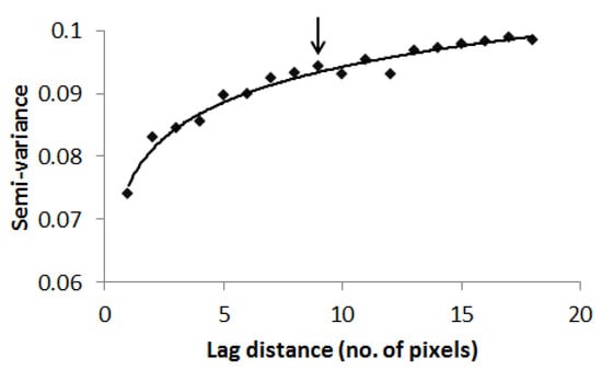
Figure 2.
Semi-variogram analysis depicting the scale of tree species diversity.
The choice for the 90 × 90 m plot size was made to record tree species diversity over space. The placement of the field plots was guided by stratified random sampling. Four dominant geological substrates (granite, siliciclastic, gabbro, and granulite) with a notable effect on plant distribution patterns in the study area were used for stratification of the sampling plots [37] (Scogings, 2004). Plots of 90 × 90 m were set up to ensure that the footprints of each plot matched with the Landsat-8 pixels. The sampling ensured that trees with a diameter at breast height (DBH) above 10 cm were documented and identified at species level. The field excursions collected tree species data in 50 plots throughout the study area. An addition of 26 field plots assembled under comparable conditions in the previous study [50] (Naidoo et al., 2015) was made. However, eight of these plots were not used because of clouds. In the end, 68 plots were considered useful in this study.
3.3. Spectral Heterogeneity Metrics
The study applied two spectral heterogeneity metrics that quantify spectral heterogeneity differently: spectral angle mapper (SAM) and coefficient of variation (CV). SAM is a mathematical algorithm that is used to select spectral bands that increase the spectral angle between target species [43,51] (Keshava, 2004; Cho et al., 2010). The spectral angle is defined as the angle () between two spectra: and
where is the number of bands.
SAM computes pairwise pixel spectral angle, using Equation (2); a larger spectral angle denotes high spectral variability between two spectra [43,51] (Keshava, 2004; Cho et al., 2010). SAM is independent of illumination variations, as it uses the angle between pixel reflectance [32] (Gholizadeh et al., 2018). Using Equation (2), SAM was applied on the Landsat-8 image in a 3 × 3 moving window to compute the inter-pixel spectral heterogeneity. Each time the 3 × 3 window moved, the average spectral angle was assigned to the center pixel. Eventually, the SAM-derived image was generated and the average spectral angle within nine pixels corresponding to the 90 × 90m field plots was extracted. SAM was calculated on each Landsat-8 image and the Landsat-derived SAM images were referred to as SAMMarch, SAMApril, SAMMay, and SAMJuly, respectively, which corresponded to each phenological date.
CV is another common spectral heterogeneity metric [30,31,32] (Torresani et al. 2019; Wang et al., 2018; Gholizadeh et al., 2018) and was computed as the mean CV for each wavelength from 442 to 2200 nm (7 bands in total).
where represents the reflectance at wavelength and and denote the standard deviation and average value of reflectance at wavelength across all the pixels in a plot, respectively.
CV was calculated using nine pixel reflectance values in each plot across all four dates studied, and these were referred to as CVMarch, CVApril, CVMay, and CVJuly, respectively. With both spectral heterogeneity metrics, higher values indicate high spectral heterogeneity, which in turn is linked to high tree species diversity.
3.4. Data Analysis
The Shannon diversity index (H′), Simpson index of diversity (D2) and species richness (S) are common measures of local diversity in the literature [33,52,53] (Lande, 1996; Colwell, 2009; Morris et al., 2014). These indices were used in this study to compute α-diversity within each plot (Table 1). Species richness is the measure of diversity that provides baseline information about the number of species in an ecosystem. Meanwhile, H′ and D2 take into account both species abundance (i.e., individual counts of trees within species) and richness (i.e., number of different tree species) when calculating species diversity [33] (Morris et al., 2014). However, there are slight differences between these two indices, with H′ containing a log function showing sensitivity to rare species, while D2 with its exponential function shows sensitivity to abundant species [34] (Nagendra, 2002).

Table 1.
Alpha diversity indices used in the study and their equations.
The study proceeded to establish 1000 random replicates of the original data set, which was divided into two-thirds for calibrating the models and one-third for validating the performance of the models. The study applied a linear regression model to investigate the relationship between the spectral heterogeneity metrics, i.e., SAM and CV, and tree species diversity as computed by the Shannon diversity index, Simpson index of diversity and species richness. r2 and p-value statistics were used to quantify the strength of the relationship statistically. Meanwhile, the accuracy of the model for prediction was assessed with the root mean square error (RMSE).
4. Results
Relationship between Tree Species Diversity and Spectral Heterogeneity
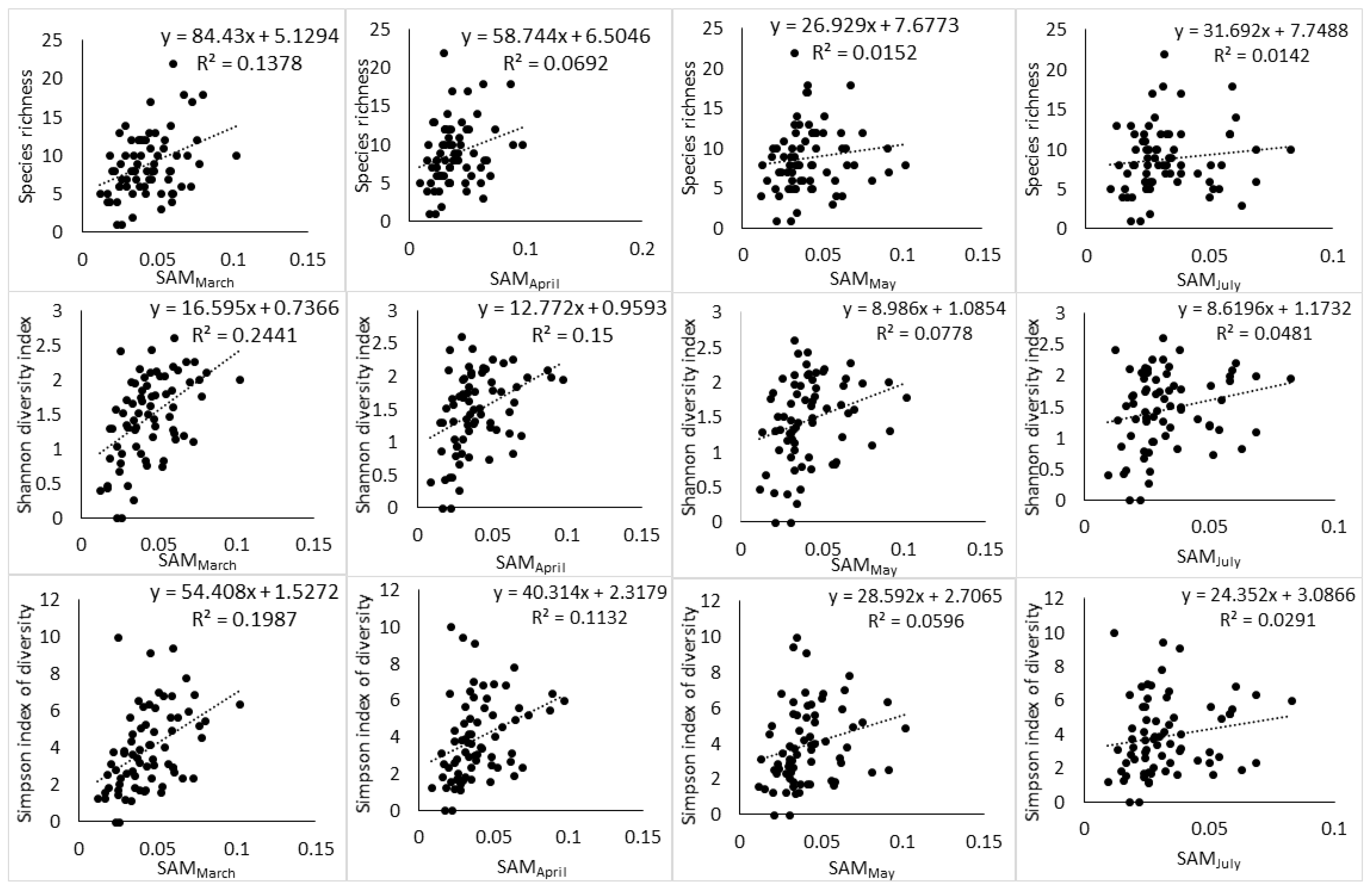
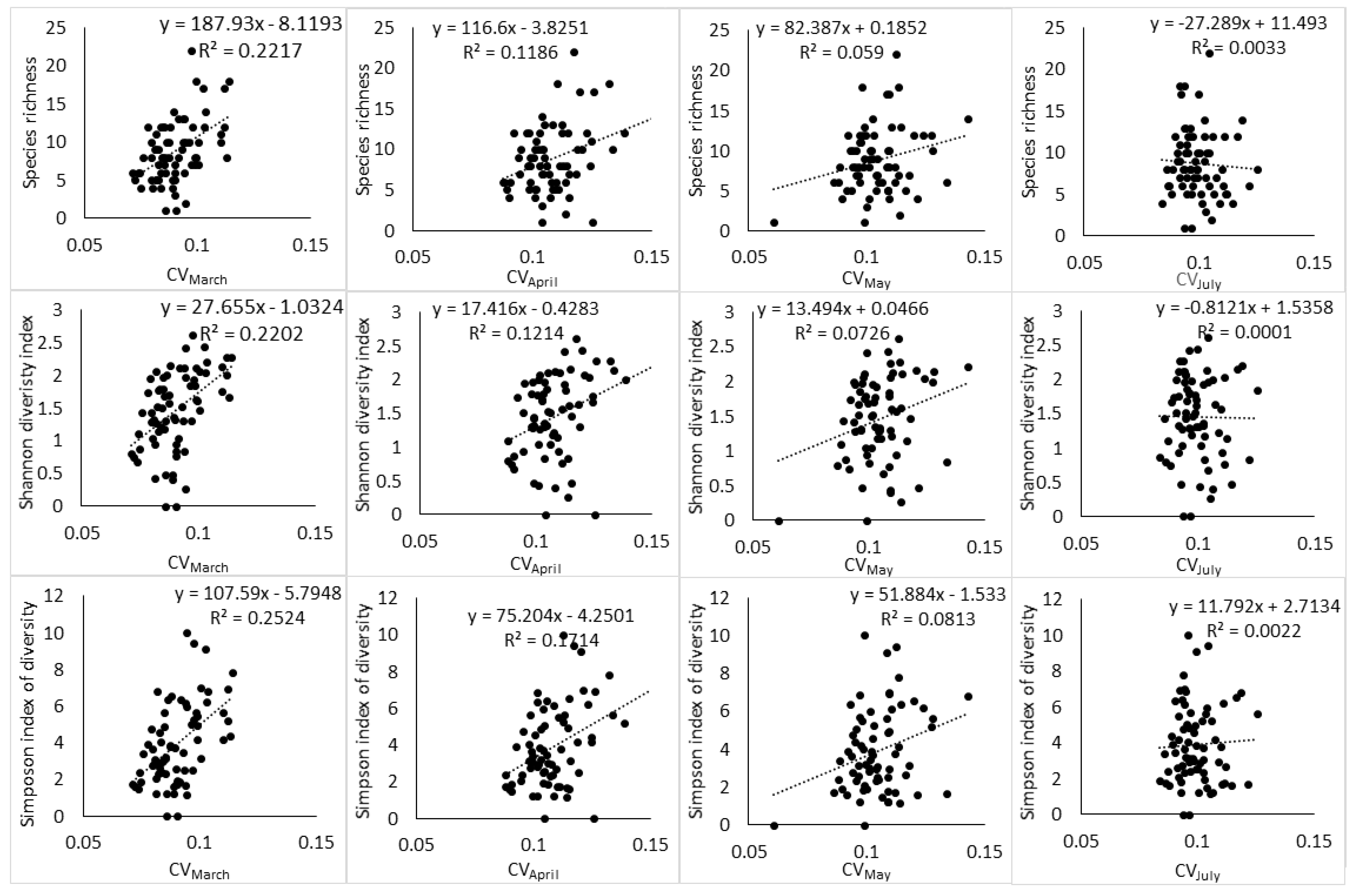
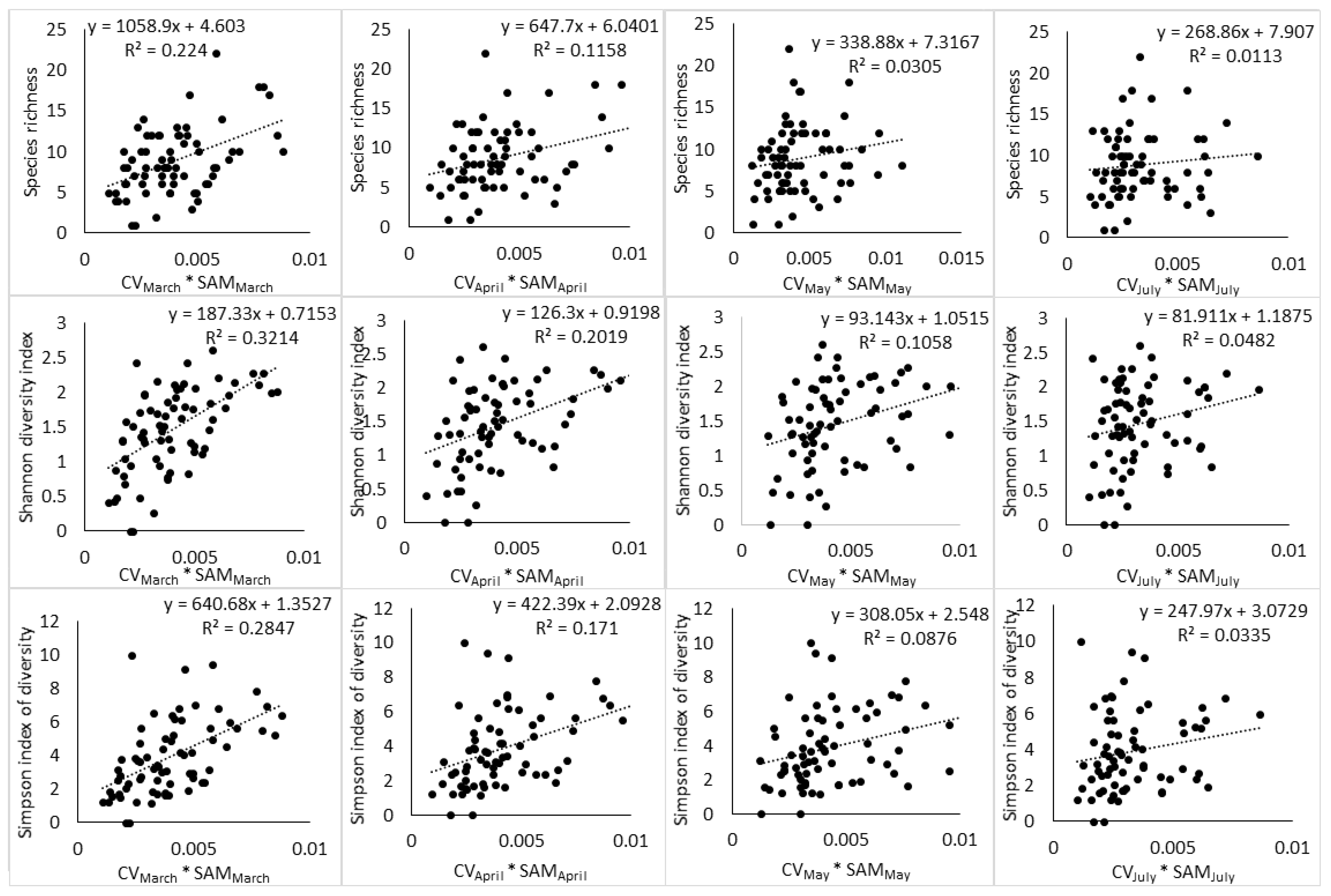
The results of regression showed that the relationship between spectral heterogeneity and tree species diversity is affected by (i) the index of species diversity used to quantify plant diversity, (ii) the spectral heterogeneity metric used to quantify spectral heterogeneity, and (iii) the phenological stage at which the image was acquired. The highest relationship between spectral heterogeneity metrics and species diversity indices was observed at the end of growing season (March) (Table 2, Table 3, Table 4, Table 5, Table 6 and Table 7). During this phenological stage, SAM and species diversity indices (S, H′, D2) had an r2 of 0.14, 0.24, 0.20, respectively, while CV had an r2 of 0.22, 0.22, and 0.25 respectively. As the phenology of vegetation transitioned toward senescence (April), advanced senescence (May) and full winter period (July), these relationships declined steadily. The interaction of SAM and CV also followed a similar phenological pattern with the end of the growing season producing higher relationship to H′ and D2 than the other phenological stages (Table 8, Table 9 and Table 10). Notably, the interaction of SAM and CV had a positive effect on the relationship between spectral heterogeneity and abundance-based diversity indices by producing an r2 of 0.32 with H′ and an r2 of 0.28 with D2 at the end of the growing season. However, the subsequent phenological stages saw the interaction of SAM and CV improving the relationship of the spectral data with H′ only. The species richness index did not benefit at all from the interaction of SAM and CV, while D2 benefited at the end of the growing season only.
Table 2.
Relationship between Landsat-8 spectral heterogeneity as computed by SAM and tree species diversity as computed by species richness (S). Statistics were extracted from 1000 bootstrapped iterations.
Table 3.
Relationship between Landsat-8 spectral heterogeneity as computed by CV and tree species diversity as computed by species richness (S). Statistics were extracted from 1000 bootstrapped iterations.
Table 4.
Relationship between Landsat-8 spectral heterogeneity as computed by SAM and tree species diversity as computed by Shannon diversity index (H′). Statistics were extracted from 1000 bootstrapped iterations.
Table 5.
Relationship between Landsat-8 spectral heterogeneity as computed by CV and tree species diversity as computed by Shannon diversity index (H′). Statistics were extracted from 1000 bootstrapped iterations.
Table 6.
Relationship between Landsat-8 spectral heterogeneity as computed by SAM and tree species diversity as computed by Simpson index of diversity (D2). Statistics were extracted from 1000 bootstrapped iterations.
Table 7.
Relationship between Landsat-8 spectral heterogeneity as computed by CV and tree species diversity as computed by Simpson index of diversity (D2). Statistics were extracted from 1000 bootstrapped iterations.
Table 8.
Relationship between SAM and CV interaction and tree species diversity as computed by species richness (S). Statistics were extracted from 1000 bootstrapped iterations.
Table 9.
Relationship between SAM and CV interaction and tree species diversity as computed by species richness (H′). Statistics were extracted from 1000 bootstrapped iterations.
Table 10.
Relationship between SAM and CV interaction and tree species diversity as computed by species richness (D2). Statistics were extracted from 1000 bootstrapped iterations.
The two spectral heterogeneity metrics showed a differential relationship to S, H′ and D2. SAM had a high relationship to H′ followed by D2 and then a lower relationship to S throughout the different phenological stages (Table 2, Table 4 and Table 6). Meanwhile, CV had a higher relationship to D2 than other plant diversity indices, and its relationship to S and H′ was approximately the same at the end of the growing season and during the transition to senescence (Table 3, Table 5 and Table 7). In addition, CV had a higher relationship to S than SAM did. In general, the results indicate that both SAM and CV had higher relationships to abundance-based indices of plant diversity than species richness. However, it was D2 that was predicted with a higher RMSE across all dates. H′ was predicted with a lower RMSE by both spectral heterogeneity metrics, and S had the second lowest RMSE across all dates.
Moreover, the relationship between spectral heterogeneity metrics and plant diversity indices showed a changing pattern with changes in phenology (Figure 3, Figure 4 and Figure 5). At the end of the growing season (March), a positive relationship can be observed with scatter points distributed evenly around the regression line. While the transition to senescence still maintains a positive relationship, the scatter points start to disintegrate away from the regression line and this disintegration gets worse as the phenology changes toward advanced senescence and the full winter period.
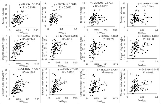
Figure 3.
Relationship between Landsat-8 spectral heterogeneity as computed by SAM and tree species diversity indices across different phenological stages.
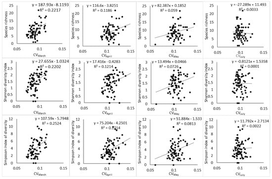
Figure 4.
Relationship between Landsat-8 spectral heterogeneity as computed by CV and tree species diversity indices across different phenological stages.
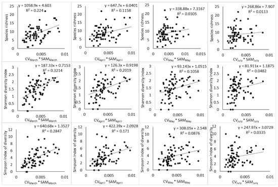
Figure 5.
Relationship between SAM and CV interaction and tree species diversity indices across different phenological stages.
5. Discussion
The results highlighted the necessity to consider vegetation phenology, spectral heterogeneity metrics and species diversity indices in the application of SVH. The results showed the declining strength of the relationships between spectral heterogeneity and plant species diversity in the African savannah with a shift in season from wet to dry; this gives an indication of the possibility of time sensitivity of the SVH. The shift from the wet to dry season is accompanied by phenological changes in the deciduous vegetation of the African savannah and this affects the spectral heterogeneity captured on the satellite data. The end of the growing season is usually characterized by fully foliated canopies in the savannah ecosystem [41] (Grant and Scholes, 2006) and therefore, tree canopies have a strong bearing on the reflectance signal captured by the sensor. This means that the spectral heterogeneity on the image acquired in the end of growing season reflects more the diversity of plant species. Meanwhile, the changes in vegetation phenology, especially toward the winter period, are associated with an increased background influence to the overall reflectance spectra recorded by the remote sensing platform as plants drop leaves [43] (Cho et al., 2010). As a result, the spectral heterogeneity on the image recorded during senescence or the dry season incorporates more background reflectance, compared to the end of the growing season. This explains the declining relationships between spectral heterogeneity metrics and plant diversity indices with a shift from the wet to dry season.
The results of the study are consistent with those of Madonsela et al. (2018) [13] in terms of the phenological effect on the modeling of tree species diversity, using remotely sensed data, even though the two studies applied different techniques. Torresani et al. (2019) [30] also observed that the relationship between spectral heterogeneity and species diversity is affected by vegetation phenology with peak summer being the most optimal phenological stage in an Italian alpine coniferous forest. Therefore, the conceptualization of SVH application in biodiversity estimation would benefit from the consideration of vegetation phenology in the study area. Figure 3 and Figure 4 showed that the phenological stage at which the satellite data are collected may partly induce confusion on the practical application of SVH. The SVH advances the argument that the spectral heterogeneity on remotely sensed image reflects spatial variation in the environment, which in turn is associated with species richness [5]. However, Schmidtlein and Fassnacht (2017) [17] observed that high spectral heterogeneity does not always correspond to high species diversity and also that low spectral heterogeneity does not always correspond to low species diversity. The results of the present study showed that phenology may be the origin of this inconsistency. At the end of growing season (Figure 3 and Figure 4), the relationship between Landsat-8 spectral heterogeneity and tree species diversity appears, to a larger extent, to be consistent with SVH. As the phenology changes toward senescence and the dry season, the relationship between Landsat-8 spectral heterogeneity and tree species diversity starts to follow the observation of Schmidtlein and Fassnacht (2017) [17] in that the spectral heterogeneity does not always correspond aptly to the observed species diversity.
Moreover, the two spectral heterogeneity metrics tested in this study, i.e., SAM and CV, showed differential relationships to S, H′ and D2, and this reflects the different ways in which the spectral heterogeneity is quantified by SAM and CV. As a result, the two metrics relate to components of plant diversity, i.e., abundance and richness in differing ways. For instance, CV had a higher relationship with S than SAM had with the same diversity index at the end of the growing season (r2 of 0.22 vs 0.13) and during the transition to senescence (r2 of 0.11 vs. 0.06). Given that S gives equal weight to rare and abundant species [56] (Daly et al., 2018), the higher relationship that CV had with S compared to SAM should be deemed to indicate its high sensitivity to rare species, while SAM can be understood to have low sensitivity to rare species. In addition, CV had similar relationships with S and H’, while SAM had higher relationships with H′ than S (Figure 3 and Figure 4) and this further illustrated the differential sensitivity to components of plant diversity. The higher relationship that SAM had with H′ compared to S indicated that the spectral heterogeneity quantified with SAM has high sensitivity to species abundance and low sensitivity to species richness.
In general, the pattern of results followed the observation of Oldeland et al. (2010) [19] and Madonsela et al. (2017) [57] regarding abundance-based indices and spectral data. The two spectral heterogeneity metrics tended to have a higher relationship with abundance-based indices of plant diversity than with S, though this occurred in the opposite manner. SAM had a higher relationship to H′ compared to other plant diversity indices, while CV had a higher relationship to D2 compared to other diversity indices. This reflects not only the differential sensitivity of spectral heterogeneity metrics to components of plant diversity, but also the variant nature in which these plant diversity components are quantified and how these indices of plant diversity relate to metrics of spectral heterogeneity. For instance, the behavior of CV seems contradictory in terms of its relationship to plant diversity indices, while SAM consistently showed bias toward abundance-based indices. CV had a higher relationship to D2 compared to other diversity indices and also a higher relationship to S than SAM had with the same diversity index. D2 places more weight on abundant species when quantifying species diversity [33] (Morris et al., 2014) while S places equal weight on both abundant species and rare species [56] (Daly et al., 2018). Therefore, if CV has high sensitivity to rare species and abundant species as the results seem to suggest, one expects it to have an even higher relationship with H’, which has high sensitivity to rare and abundant species. Yet, the relationship that CV had with H′ was no better than that which it had with S.
Interestingly, the interaction of SAM and CV improved the relationship that spectral data had with H′ and D2 at the end of the growing season (Figure 5) and further improvement were noted with H′ in the transition to senescence and during the advanced senescence period. In the meanwhile, the interaction of SAM and CV did not improve the relationship between the spectral data and S. These observations imply that each spectral heterogeneity metric has high sensitivity to a particular component of plant diversity and their interaction increased the relationship between the spectral data and abundance-based indices, especially H’, which has high sensitivity to rare and abundant species [33] (Morris et al., 2014).
Overall, the study showed a glimpse that SVH could be implemented to characterize tree species diversity in southern African savannahs, especially at the end of the growing season. Even though the coefficient of determination was comparatively low, the relationship between spectral heterogeneity and tree species diversity was statistically significant (p < 0.05), except during the dry season. However, there are still challenges to the accurate modeling of tree species diversity in the savannahs following the SVH concept. Savannah vegetation is characterized by the co-occurrence of trees, grasses and pockets of bare areas [20,58] (Scholes and Archer, 1997; Scalon et al., 2002). Trees and grasses have been observed to follow different phenological pathways in the savannah [59] (Archibald and Scholes, 2007) and differences in vegetation phenology tend to increase spectral heterogeneity [26,28] (Gilmore et al., 2008; Hill et al., 2010). In such circumstances, spectral heterogeneity may not only be the consequence of tree species diversity. Instead, it may be a reflection of discrepancies in vegetation cover. For instance, Oldeland et al. (2010) [19] observed that high spectral heterogeneity does not always correspond to high plant diversity in the savannah, and that was due to the disparity in vegetation cover.
6. Conclusions
The study concludes that vegetation phenology affects the relationship between spectral heterogeneity and plant species diversity. In this study, the end of the growing season was the optimal phenological stage where the relationships between spectral heterogeneity metrics and species diversity indices were high, and it declined steadily with changes in phenology toward senescence. This observation gives an indication that SVH might be time dependent and therefore, vegetation phenology ought to be considered in the application of SVH for biodiversity estimation. Moreover, the choice of spectral heterogeneity metrics and species diversity indices affects the success of SVH application. The two spectral heterogeneity metrics adopted in this study showed differential relationships to species diversity indices, and this highlights the difference in the manner in which spectral heterogeneity is computed between the two metrics as well as the difference in how components of species diversity are quantified by different diversity indices. In general, the two metrics had high relationships to H′ and D2, which are abundance-based indices of species diversity. In fact, the interaction of these spectral heterogeneity metrics improved the relationship between the spectral data and abundance-based indices, especially H’, which saw improvement at different phenological stages. However, CV improved the relationship between spectral data and S, and this is worth emphasizing, given that S provides baseline information on biodiversity. All of these observations suggest that the choice of spectral heterogeneity metric should be made in line with the purpose of SVH application since these metrics relate to components of species diversity differently.
Author Contributions
Conceptualization, S.M. and M.A.C.; methodology, S.M.; validation, M.A.C., A.R. and O.M.; formal analysis, S.M.; investigation, S.M.; resources, M.A.C.; data curation, S.M.; writing—original draft preparation, S.M.; writing—review and editing, S.M. and A.R.; visualization, SM.; supervision, M.A.C., A.R. and O.M.; project administration, M.A.C.; funding acquisition, M.A.C. All authors have read and agreed to the published version of the manuscript.
Funding
This study was funded by the National Research Foundation (NRF) through the NRF-Professional Development Programme.
Institutional Review Board Statement
Not applicable.
Informed Consent Statement
Not applicable.
Data Availability Statement
The data presented in this study are available on request from the corresponding author. The data are not publicly available as it is still used for further research in the study area.
Acknowledgments
The authors are grateful to Cecilia Masemola, Sbu Gumede, Joseph Dlamini, Martin Sarela and Patrick Ndlovu for their support during the collection of field data. The authors are thankful to Laven Naidoo for editing our use of the English language.
Conflicts of Interest
The authors declare no conflict of interest.
References
- Turner, W.; Spector, S.; Gardiner, N.; Fladeland, M.; Sterling, E.; Steininger, M. Remote sensing for biodiversity science and conservation. Trends Ecol. Evol. 2003, 18, 306–314. [Google Scholar] [CrossRef]
- Kerr, J.T.; Ostrovsky, M. From space to species: Ecological applications for remote sensing. Trends Ecol. Evol. 2003, 18, 299–305. [Google Scholar] [CrossRef]
- Warren, S.D.; Alt, M.; Olson, K.D.; Irl, S.D.; Steinbauer, M.J.; Jentsch, A. The relationship between the spectral diversity of satellite imagery, habitat heterogeneity, and plant species richness. Ecol. Inform. 2014, 24, 160–168. [Google Scholar] [CrossRef]
- Rocchini, D.; Boyd, D.; Féret, J.; Foody, G.; He, K.S.; Lausch, A.; Nagendra, H.; Wegmann, M.; Pettorelli, N. Satellite remote sensing to monitor species diversity: Potential and pitfalls. Remote. Sens. Ecol. Conserv. 2016, 2, 25–36. [Google Scholar] [CrossRef]
- Palmer, M.W.; Earls, P.G.; Hoagland, B.W.; White, P.S.; Wohlgemuth, T. Quantitative tools for perfecting species lists. Environmetrics 2002, 13, 121–137. [Google Scholar] [CrossRef]
- Fairbanks, D.H.K.; McGwire, K.C. Patterns of floristic richness in vegetation communities of California: Regional scale analysis with multi-temporal NDVI. Glob. Ecol. Biogeogr. 2004, 13, 221–235. [Google Scholar] [CrossRef]
- Gould, W. Remote sensing of vegetation, plant species richness, and regional biodiversity hotspots. Ecol. Appl. 2000, 10, 1861–1870. [Google Scholar] [CrossRef]
- He, K.S.; Zhang, J.; Zhang, Q. Linking variability in species composition and MODIS NDVI based on betadiversity measurements. Acta Oecol. 2009, 35, 14–21. [Google Scholar] [CrossRef]
- Oindo, B.O.; Skidmore, A.K. Interannual variability of NDVI and species richness in Kenya. Int. J. Remote Sens. 2002, 23, 285–298. [Google Scholar] [CrossRef] [Green Version]
- Parviainen, M.; Luoto, M.; Heikkinen, R.K. NDVI-based productivity and heterogeneity as indicators of plant-species richness in boreal landscapes. Boreal Environ. Res. 2010, 15, 301–318. [Google Scholar]
- Witman, J.D.; Cusson, M.; Archambault, P.; Pershing, A.J.; Mieszkowska, N. The relation between productivity and species diversity in temperate–Arctic marine ecosystems. Ecology 2008, 89, S66–S80. [Google Scholar] [CrossRef] [Green Version]
- Pau, S.; Gillespie, T.W.; Wolkovich, E.M. Dissecting NDVI-species richness relationships in Hawaiian dry forests. J. Biogeogr. 2012, 39, 1678–1686. [Google Scholar] [CrossRef]
- Madonsela, S.; Cho, M.A.; Ramoelo, A.; Mutanga, O.; Naidoo, L. Estimating tree species diversity in the savannah using NDVI and woody canopy cover. Int. J. Appl. Earth Obs. Geoinf. 2018, 66, 106–115. [Google Scholar] [CrossRef] [Green Version]
- Stein, A.; Gerstner, K.; Kreft, H. Environmental heterogeneity as a universal driver of species richness across taxa, biomes and spatial scales. Ecol. Lett. 2014, 17, 866–880. [Google Scholar] [CrossRef] [PubMed]
- Rocchini, D.; Balkenhol, N.; Carter, G.A.; Foody, G.; Gillespie, T.W.; He, K.S.; Kark, S.; Levin, N.; Lucas, K.; Luoto, M.; et al. Remotely sensed spectral heterogeneity as a proxy of species diversity: Recent advances and open challenges. Ecol. Inform. 2010, 5, 318–329. [Google Scholar] [CrossRef]
- Féret, J.-B.; Asner, G.P. Mapping Tropical Forest Canopy Diversity Using High-fidelity Imaging Spectroscopy. Ecol. Appl. Publ. Ecol. Soc. Am. 2014, 24, 1289–1296. [Google Scholar] [CrossRef] [PubMed]
- Schmidtlein, S.; Fassnacht, F.E. The spectral heterogeneity hypothesis does not hold across landscapes. Remote Sens. Environ. 2017, 192, 114–125. [Google Scholar] [CrossRef] [Green Version]
- Schweiger, A.K.; Cavender-Bares, J.; Townsend, P.A.; Hobbie, S.E.; Madritch, M.D.; Wang, R.; Tilman, D.; Gamon, J.A. Plant Spectral Diversity Integrates Functional and Phylogenetic Components of Biodiversity and Predicts Ecosystem Function. Nat. Ecol. Evol. 2018, 2, 976–982. [Google Scholar] [CrossRef] [PubMed]
- Oldeland, J.; Wesuls, D.; Rocchini, D.; Schmidt, M.; Jürgens, N. Does using species abundance data improve estimates of species diversity from remotely sensed spectral heterogeneity? Ecol. Indic. 2010, 10, 390–396. [Google Scholar] [CrossRef]
- Scholes, R.J.; Archer, S.R. Tree-Grass Interactions in Savannas. Annu. Rev. Ecol. Syst. 1997, 28, 517–544. [Google Scholar] [CrossRef]
- Rocchini, D.; Chiarucci, A.; Loiselle, S. Testing the spectral variation hypothesis by using satellite multispectral images. Acta Oecologica 2004, 26, 117–120. [Google Scholar] [CrossRef]
- González-Megías, A.; María Gómez, J.; Sánchez-Piñero, F. Diversity-habitat heterogeneity relationship at different spatial and temporal scales. Ecography 2007, 30, 31–41. [Google Scholar] [CrossRef]
- Rocchini, D. Effects of spatial and spectral resolution in estimating ecosystem α-diversity by satellite imagery. Remote. Sens. Environ. 2007, 111, 423–434. [Google Scholar] [CrossRef]
- Gholizadeh, H.; Gamon, J.A.; Helzer, C.J.; Cavender-Bares, J. Multi-temporal assessment of grassland α-and β-diversity using hyperspectral imaging. Ecol. Appl. 2020, 30, e02145. [Google Scholar] [CrossRef] [PubMed]
- Flanagan, L.B.; Sharp, E.J.; Gamon, J.A. Application of the photosynthetic light-use efficiency model in a northern Great Plains grassland. Remote. Sens. Environ. 2015, 168, 239–251. [Google Scholar] [CrossRef]
- Hill, R.A.; Wilson, A.; George, M.; Hinsley, S. Mapping tree species in temperate deciduous woodland using time-series multi-spectral data. Appl. Veg. Sci. 2010, 13, 86–99. [Google Scholar] [CrossRef]
- Lopes, M.; Fauvel, M.; Ouin, A.; Girard, S. Spectro-Temporal Heterogeneity Measures from Dense High Spatial Resolution Satellite Image Time Series: Application to Grassland Species Diversity Estimation. Remote. Sens. 2017, 9, 993. [Google Scholar] [CrossRef] [Green Version]
- Gilmore, M.S.; Wilson, E.H.; Barrett, N.; Civco, D.L.; Prisloe, S.; Hurd, J.D.; Chadwick, C. Integrating multi-temporal spectral and structural information to map wetland vegetation in a lower Connecticut River tidal marsh. Remote. Sens. Environ. 2008, 112, 4048–4060. [Google Scholar] [CrossRef]
- Madonsela, S.; Cho, M.A.; Mathieu, R.; Mutanga, O.; Ramoelo, A.; Kaszta, Ż; Van De Kerchove, R.; Wolff, E. Multi-phenology WorldView-2 imagery improves remote sensing of savannah tree species. Int. J. Appl. Earth Obs. Geoinf. 2017, 58, 65–73. [Google Scholar] [CrossRef] [Green Version]
- Torresani, M.; Rocchini, D.; Sonnenschein, R.; Zebisch, M.; Marcantonio, M.; Ricotta, C.; Tonon, G. Estimating tree species diversity from space in an alpine conifer forest: The Rao’s Q diversity index meets the spectral variation hypothesis. Ecol. Inform. 2019, 52, 26–34. [Google Scholar] [CrossRef] [Green Version]
- Wang, R.; Gamon, J.A.; Wang, R.; Gamon, J.A.; Cavender-Bares, J.; Townsend, P.A.; Zygielbaum, A.I. The spatial sensitivity of the spectral het-erogeneity–biodiversity relationship: An experimental test in a prairie grassland. Ecol. Appl. 2018, 28, 541–556. [Google Scholar] [CrossRef] [Green Version]
- Gholizadeh, H.; Gamon, J.A.; Zygielbaum, A.I.; Wang, R.; Schweiger, A.K.; Cavender-Bares, J. Remote sensing of bio-diversity: Soil correction and data dimension reduction methods improve assessment of α-diversity (species richness) in prairie ecosystems. Remote. Sens. Environ. 2018, 206, 240–253. [Google Scholar] [CrossRef]
- Morris, E.K.; Caruso, T.; Buscot, F.; Fischer, M.; Hancock, C.; Maier, T.S.; Meiners, T.; Müller, C.; Obermaier, E.; Prati, D.; et al. Choosing and using diversity indices: Insights for ecological applications from the German Biodiversity Exploratories. Ecol. Evol. 2014, 4, 3514–3524. [Google Scholar] [CrossRef] [PubMed] [Green Version]
- Nagendra, H. Opposite trends in response for the Shannon and Simpson indices of landscape diversity. Appl. Geogr. 2002, 22, 175–186. [Google Scholar] [CrossRef]
- Sankaran, M.; Hanan, N.; Scholes, R.J.; Ratnam, J.; Augustine, D.; Cade, B.S.; Gignoux, J.; Higgins, S.I.; Le Roux, X.; Ludwig, F.; et al. Determinants of woody cover in African savannas. Nat. Cell Biol. 2005, 438, 846–849. [Google Scholar] [CrossRef]
- Bond, W.J.; Midgley, G.F.; Woodward, F.I. The importance of low atmospheric CO2 and fire in promoting the spread of grasslands and savannas. Glob. Chang. Biol. 2003, 9, 973–982. [Google Scholar] [CrossRef]
- Scogings, P.F. The Kruger Experience: Ecology and Management of Savanna Heterogeneity–Johan du Toit, Kevin Rogers and Harry Biggs (eds) 2003. Afr. J. Range Forage Sci. 2004, 21, 67. [Google Scholar] [CrossRef]
- Eckhardt, H.C.; Van Wilgen, B.W.; Biggs, H.C.; Eckhardt, H.C.; Van Wilgen, B.W.; Biggs, H.C. Trends in woody vegetation cover in the Kruger National Park, South Africa, between 1940 and 1998. Afr. J. Ecol. 2000, 38, 108–115. [Google Scholar] [CrossRef]
- Makhado, R.A.; Mapaure, I.; Potgieter, M.J.; Luus-Powell, W.J.; Saidi, A.T. Factors influencing the adaptation and distribution of Colophospermum mopane in southern Africa’s mopane savannas-A review. Bothalia-Afr. Biodivers. Conserv. 2014, 44, 1–9. [Google Scholar] [CrossRef]
- Pervaiz, W.; Uddin, V.; Khan, S.A.; Khan, J.A. Satellite-based land use mapping: Comparative analysis of Landsat-8, Advanced Land Imager, and big data Hyperion imagery. J. Appl. Remote Sens. 2016, 10, 026004. [Google Scholar] [CrossRef] [Green Version]
- Grant, C.; Scholes, M. The importance of nutrient hot-spots in the conservation and management of large wild mammalian herbivores in semi-arid savannas. Biol. Conserv. 2006, 130, 426–437. [Google Scholar] [CrossRef]
- Scholes, R.J.; Bond, W.J.; Eckhardt, H.C. Vegetation dynamics in the Kruger ecosystem. In The Kruger Experience: Ecology and Management of Savanna Heterogeneity; Island Press: Washington, DC, USA, 2013; pp. 242–262. [Google Scholar]
- Cho, M.A.; Debba, P.; Mathieu, R.; Naidoo, L.; Van Aardt, J.; Asner, G. Improving Discrimination of Savanna Tree Species Through a Multiple-Endmember Spectral Angle Mapper Approach: Canopy-Level Analysis. IEEE Trans. Geosci. Remote. Sens. 2010, 48, 4133–4142. [Google Scholar] [CrossRef]
- Kaszta, Ż.; Van De Kerchove, R.; Ramoelo, A.; Cho, M.; Madonsela, S.; Mathieu, R.; Wolff, E. Seasonal separation of African savanna components using worldview-2 imagery: A comparison of pixel-and object-based approaches and selected classifica-tion algorithms. Remote Sens. 2016, 8, 763. [Google Scholar] [CrossRef] [Green Version]
- Richter, R.; Schläpfer, D. Atmospheric/Topographic Correction for Satellite Imagery; DLR Report; DLR—German Aerospace Center: Köln, Germany, 2015; Volume 565. [Google Scholar]
- Gringarten, E.; Deutsch, C. Teacher’s Aide Variogram Interpretation and Modeling. Math. Geol. 2001, 33, 507–534. [Google Scholar] [CrossRef]
- Fu, W.J.; Jiang, P.K.; Zhou, G.M.; Zhao, K.L. Using Moran’s I and GIS to study the spatial pattern of forest litter carbon density in a subtropical region of southeastern China. Biogeosciences 2014, 11, 2401–2409. [Google Scholar] [CrossRef] [Green Version]
- Jongman, E.; Jongman, S.R.R. Data Analysis in Community and Landscape Ecology; Cambridge University Press: Cambridge, UK, 1995. [Google Scholar]
- Cho, M.A.; Mathieu, R.; Asner, G.; Naidoo, L.; Van Aardt, J.; Ramoelo, A.; Debba, P.; Wessels, K.; Main, R.; Smit, I.P.; et al. Mapping tree species composition in South African savannas using an integrated airborne spectral and LiDAR system. Remote. Sens. Environ. 2012, 125, 214–226. [Google Scholar] [CrossRef]
- Naidoo, L.; Mathieu, R.; Main, R.; Kleynhans, W.; Wessels, K.; Asner, G.; Leblon, B. Savannah woody structure modelling and mapping using multi-frequency (X-, C- and L-band) Synthetic Aperture Radar data. ISPRS J. Photogramm. Remote. Sens. 2015, 105, 234–250. [Google Scholar] [CrossRef] [Green Version]
- Keshava, N. Distance metrics and band selection in hyperspectral processing with applications to material identification and spectral libraries. IEEE Trans. Geosci. Remote. Sens. 2004, 42, 1552–1565. [Google Scholar] [CrossRef]
- Colwell, R.K. III. 1 Biodiversity: Concepts, Patterns, and Measurement. In The Princeton Guide to Ecology; Walter de Gruyter GmbH: Berlin, Germany, 2009; pp. 257–263. [Google Scholar]
- Lande, R. Statistics and Partitioning of Species Diversity, and Similarity among Multiple Communities. Oikos 1996, 76, 5–13. [Google Scholar] [CrossRef]
- Shannon, C.E. A mathematical theory of communication. Bell Syst. Tech. J. 1948, 27, 379–423. [Google Scholar] [CrossRef] [Green Version]
- Simpson, E. Measurement of diversity. Nature 1949, 163, 688. [Google Scholar] [CrossRef]
- Daly, A.J.; Baetens, J.M.; De Baets, B. Ecological Diversity: Measuring the Unmeasurable. Mathematics 2018, 6, 119. [Google Scholar] [CrossRef] [Green Version]
- Madonsela, S.; Cho, M.A.; Ramoelo, A.; Mutanga, O. Remote sensing of species diversity using Landsat 8 spectral variables. ISPRS J. Photogramm. Remote. Sens. 2017, 133, 116–127. [Google Scholar] [CrossRef] [Green Version]
- Scanlon, T.M.; Albertson, J.D.; Caylor, K.K.; Williams, C. Determining land surface fractional cover from NDVI and rainfall time series for a savanna ecosystem. Remote. Sens. Environ. 2002, 82, 376–388. [Google Scholar] [CrossRef]
- Archibald, S.; Scholes, R.J. Leaf green-up in a semi-arid African savanna -separating tree and grass responses to environmental cues. J. Veg. Sci. 2007, 18, 583–594. [Google Scholar]
Publisher’s Note: MDPI stays neutral with regard to jurisdictional claims in published maps and institutional affiliations. |
© 2021 by the authors. Licensee MDPI, Basel, Switzerland. This article is an open access article distributed under the terms and conditions of the Creative Commons Attribution (CC BY) license (https://creativecommons.org/licenses/by/4.0/).