Tropical Cyclone Center Positioning Using Single Channel Microwave Satellite Observations of Brightness Temperature

Abstract

Satellite observations of brightness temperature from the Advanced Technology Microwave Sounder (ATMS) and Microwave Humidity Sounder (MHS) humidity sounding channels can provide relatively high horizontal resolution information about cloud and atmospheric moisture in the troposphere, thus revealing the structures of tropical cyclones (TCs). There is usually a high brightness temperature in a TC eye region and low brightness temperature reflecting spiral rain bands. An azimuthal spectral analysis method is used as a center-fixing algorithm to determine the TC center objectively using the brightness temperature observations of the ATMS humidity-sounding channel 18 (183.31 ± 7.0 GHz) and MHS humidity-sounding channel 5 (190.31 GHz). The position in the brightness temperature field encompassing a TC that achieves the largest symmetric component is regarded as the TC center. Two Atlantic hurricanes in 2012, Hurricanes Sandy and Isaac, are first used to analyze the performance of the TC center-fixing technique. Compared with the National Hurricane Center best track, the root-mean-square differences of the center fixing results for Hurricanes Sandy and Isaac are less than 47.3 and 34.3 km, respectively. It is found that the uncertainty of the TC center-fixing algorithm and thus the difference from the best track increases when the brightness temperature distribution within a TC is significantly asymmetric. Then, the TC center-fixing technique is validated for all tropical storms and hurricanes over Northern Atlantic and Western Pacific in 2019. Compared with the best track data, the root-mean-square differences for tropical storms and hurricanes are 33.81 and 26.20 km, respectively. The demonstrated successful performance of the proposed TC center-fixing algorithm to use the single channel of microwave humidity sounders for TC positioning is important for vortex initialization in operational hurricane forecasts.

1. Introduction

Locating the center of a TC is an essential step in the operational forecasting and analysis of TC. The location of the TC center is a key parameter required for the initialization of the TC numerical forecast model. An incorrect initial position of the TC center will reduce the forecast skill of the TC track and intensity [1,2,3,4]. At present, the most commonly used data source for locating the TC center is satellite observations. Meteorological satellites have provided abundant infrared, visible, and microwave observations, which are particularly valuable in data-sparse regions such as the tropics.

The mainstream method of TC center positioning comes from Dvorak Technology (DT) [5,6]. DT is a well-known technique for estimating the TC position and intensity, which has undergone a series of improvements. In the early version of DT, the geostationary satellite infrared images were matched with some summarized conceptual templates of cloud eyes and spiral cloud bands at different development stages of TC, combined with a series of empirical rules and constraints to determine the cloud system center (CSC) manually. The CSC was regarded as the TC center. The conceptual templates of TC can be divided into cloud eye templates and non-cloud eye templates. The TC templates with cloud eye have the shapes of round eye, oval eye, semi-circular eye, irregular eye, broken eye, etc. The CSC is the center of the cloud eye or at the center of curvature of a partial eyewall. The TC templates without cloud eye include types of curved band pattern, Central Dense Overcast (CDO) pattern, and shear pattern. The CSC is the common center of curvature of curved cloud bands or the center of the CDO. Velden et al. (1998) [7] improved the TC intensity estimation part in DT by changing it to a computer-based objective estimation technology, which is called the Objective Dvorak Technique (ODT). The determination of TC center positioning remained manually in the ODT. Subsequently, Wimmers and Velden (2004) [8] proposed an objective TC center positioning method combining the so-called spiral centering (SC) and the ring fitting (RF) techniques, which was known as the SC-RF TC positioning technique in the Advanced Objective Dvorak Technique (AODT) [9,10] and the Advanced Dvorak Technique (ADT) [4]. The SC technique determines the TC center position by calculating the maximum alignment between the gradient field of satellite brightness temperature and a specified spiral-shaped unit vector field. The RF technique further modifies the SC-determined TC center position by calculating the fitting degree between the gradient field of brightness temperature around the SC-determined TC center position and a given ring pattern representing the TC eyewall inner edge if it appears. The SC-RF method was later developed into an automated and objective TC center-fixing algorithm called the Automated Rotational Center Hurricane Eye Retrieval (ARCHER) algorithm [11,12]. The ARCHER algorithm realized SC and RF techniques by calculating the spiral score (FSS) and ring score (RS) at all data points of brightness temperature, whose weighted sum is defined as the combined score (CS). The position with the highest CS refers to the TC center position determined by the AECHER algorithm. The ARCHER algorithm is applicable to a variety of satellite observations, including the brightness temperature observations of infrared, visible, 85–92- and 37-GHz microwave sounding channels and the ambiguity vectors of scatterometer retrievals.

So far, the geostationary visible and infrared observations with high temporal resolution are still the primary tool for TC center positioning. However, due to the weak ability of infrared radiations to penetrate clouds and the limitation of visible channels at night-times, it is difficult to detect the complete TC structure when it is obscured by higher clouds (such as cirrus). Microwave radiations with a wide range of wavelengths from microwave sounders onboard polar-orbiting operational environmental satellites can penetrate cirrus and discern structures of TC in the middle and lower troposphere. When the ARCHER algorithm was applied to the brightness temperature field of the longwave infrared channel 89 (703.75 cm⁻¹) of Cross-Track Infrared Sounder (CrIS) and the humidity-sounding channel 22 (183.31 ± 1.0 GHz) of the ATMS onboard the Suomi National Polar-orbiting Partnership (S-NPP) satellite, it was found that the small-scale convective cloud features in the brightness temperature field of the ATMS channel 22 interfered with the TC rotational center, which increased the positioning errors [13]. Hu and Zou [13] proposed a method first to determine the initial position of the TC center by the ARCHER algorithm using the ATMS temperature channel 4 with a coarse observation resolution, and then to perform a series of azimuthal spectral analyses centered on positions near the initial position of TC center in the brightness temperature field of the ATMS humidity-sounding channel 22 with a fine observation resolution. The center location of the azimuthal spectral analysis corresponding to the largest symmetric (wavenumber—0) component of the brightness temperature field was selected as the final position of TC center. The TC center-fixing method proposed in this paper discards the first step involving the ARCHER algorithm and directly applies the azimuthal spectral analysis method to the field of brightness temperature from a single microwave channel—the ATMS humidity-sounding channel 18 (183.31 ± 7.0 GHz) or the MHS humidity-sounding channel 5 (190.31 GHz). The weighting functions of the two humidity-sounding channels peak at about 800 hPa under clear-sky conditions [14], which allows them to provide detailed information about water vapor structures around the TC in the low troposphere. Although a microwave humidity sounder onboard a single polar-orbiting operational environmental satellite can only observe the same TC twice daily at most, the ATMS onboard the S-NPP and NOAA-20 satellites, MHS onboard NOAA and MetOp satellites, and microwave humidity sounder (MWHS) onboard the FY-3C and FY-3D have similar sounding characteristics, and the combination of them can improve the temporal resolutions of TC.

In addition to satellite data, there are also radar data, aerial reconnaissance data, land observations and ship reports, etc., which are also used for TC center positioning. For example, using radar data (reflectivity, radial velocity measured by Doppler radar, wind field collected by airborne Doppler radar, etc.), the geometric center of the eye of a TC nearing land was taken as the TC center [15,16,17,18,19]. The TC center position determined by the aerial reconnaissance data was defined as the location of the wind speed minimum or wind shift encountered along the flight path. However, locating the TC center by aircraft or radar has limitations in terms of the detection distance and observation range, while satellite observations are not subject to this limitation, and it has been and will be more widely used in TC center positioning.

The post-TC center position data can be found in the best track from the National Hurricane Center (NHC) and Joint Typhoon Warning Center (JTWC), which are provided every six hours and refer to the TC center position at the sea surface. However, the best track generally has a time lag of months or even a year. The TC positioning method proposed in this paper can locate the TC center position rapidly and in real time.

The article is organized as follows. Section 2 briefly describes the ATMS and MHS instrument channel characteristics, the NHC best track, and TC cases. Section 3 gives details about the azimuthal spectral analysis method for determining the TC center using brightness temperature observations of a single microwave humidity sounding channel. Section 4 discusses the center-positioning results of Hurricane Sandy and shows its structural evolution along the track in microwave observations of the ATMS and MHS. In Section 5, the center-positioning results of Hurricane Isaac are provided. Section 6 provides validation results of the TC center-positioning technique for all tropical storms and hurricanes over the Atlantic and Pacific oceans in 2019. Section 7 and Section 8 present a discussion and conclusions, respectively.

2. Data and TC Case Description

2.1. ATMS and MHS Channel Characteristics and Best Track Description

The ATMS onboard the S-NPP satellite is a newly developed cross-track microwave radiometer after the Advanced Microwave Sounding Unit-A (AMSU-A) and MHS onboard NOAA and MetOp satellites. It inherits and combines most of the sounding channels from these two predecessors [14]. The ATMS temperature sounding channels 1–3 and 5–15 have the same frequencies as AMSU-A channels 1–14, which can provide atmospheric temperature information as well as clouds and surface conditions. The ATMS humidity sounding channels 20 and 22 have the same frequencies as MHS channels 4 and 3, and the ATMS channels 17 (165.5 GHz) and 18 (183.31 ± 7.0 GHz) have slightly different frequencies from MHS channels 2 (157.0 GHz) and 5 (190.31 GHz). The ATMS and MHS humidity sounding channels are designed for probing atmospheric moisture in the troposphere below ~200 hPa. The ATMS temperature channel 4 (51.76 GHz) and humidity channels 19 (183.31 ± 4.5 GHz) and 21 (183.31 ± 1.8 GHz), which are not available from AMSU-A and MHS, are unique for better profiling atmospheric temperature and moisture profiles. The ATMS humidity channels 17–22 and MHS channels 1–5 have the same beam width of 1.1°, and therefore the same size of field-of-view (FOV). The diameter of the FOV at nadir is 16 km. In this study, the ATMS channel 18 and the MHS channel 5, whose weighting functions peak at about 800 hPa, were selected to locate the TC center. The two humidity sounding channels can provide detailed moisture structural distributions in the lower troposphere, especially for the storm conditions, while being less affected by surface conditions than window channels.

The TC center positions from the National Hurricane Center best track are used to examine the accuracy of ATMS- or MHS-determined TC centers. The best track provides positions, intensities, central pressures, and sizes of post-TCs every six hours. It utilizes almost all available observations of the relevant TC. The average best track uncertainty for position with only satellite observations was about 63.9, 43.0, and 22.8 km for tropical storms, category 1 and 2 hurricanes, and major hurricanes, respectively [20]. The uncertainty would be reduced to 40.7, 27.6, and 20.7 km with the inclusion of aircraft reconnaissance observations [20].

2.2. TC Case Description

Hurricanes Sandy and Isaac that occurred in 2012 over the Atlantic Ocean are selected for a detailed investigation in this study. Hurricane Sandy’s northward track was mainly caused by steering wind associated with the large-scale trough and ridge systems, while hurricane Isaac has a typical northwestward track in the Northern Hemisphere. The temporal evolutions of the best track and the maximum sustained wind and minimum central pressure of Hurricanes Sandy and Isaac during their entire lifetimes are shown in Figure 1. Hurricane Sandy developed from a tropical wave in the southwestern Caribbean Sea and further developed into a tropical storm on 22 October 2012. Sandy then intensified at a fast pace and became a category 1–2 hurricane after 24 October. Sandy initially moved roughly northward over Cuba and the Bahamas and northeastward when entering middle latitudes at about 1800 UTC 26 October, and finally northwestward after 0600 UTC 29 October. It made landfall on 30 October near Atlantic City. Sandy has a primary peak intensity of about 50 m·s⁻¹ at 0600 UTC 25 October and a secondary peak intensity of about 42.5 m·s⁻¹ at 1200 UTC 29 October 2012 (Figure 1a,b). Hurricane Isaac originated from a tropical wave in the west coast of Africa on 21 August 2012 and developed into a tropical storm later. Isaac moved initially westward before 24 August and northwestward after that day, and eventually made landfall in southeastern Louisiana on 29 August. Isaac was a tropical storm for most of its life except around October 29 when it reached a category-1 hurricane (about 35 m·s⁻¹) a few hours before landfalling (Figure 1a,c).

Hurricane tracks are mostly affected by the environmental steering flow, which is defined as the deep-layer mean wind within an area centered on the TC center (Figure 2). The deep-layer mean wind was calculated by the following formula [21,22]:

$$u_{mean}=\frac{75u_{300}+100u_{400}+150u_{500}+175u_{600}+175u_{700}+150u_{850}}{825}$$

(1)

$$v_{mean}=\frac{75v_{300}+100v_{400}+150v_{500}+175v_{600}+175v_{700}+150v_{850}}{825}$$

(2)

where $u_{mean}$ and $v_{mean}$ are zonal (u) and meridional (v) wind components of deep-layer mean wind. $u_{300–850}$ and $v_{300–850}$ are U- and V-components of wind from ERA5 reanalysis at 300–850 hPa with a 0.25° × 0.25^° grid. The environmental steering flow and thus the track were closely associated with the weather systems in the surrounding environment of Hurricane Sandy. We show in Figure 2 the steering flow as well as the potential vorticity and geopotential height at 200 hPa at eight selected times during the lifespan of Sandy. Before 23 October 2012, Sandy moved slowly toward the west and southwest in an environment associated with an upper-level anticyclone over the southwestern Caribbean Sea. An upper-level trough over the northwestern Caribbean Sea and Gulf of Mexico caused Sandy to accelerate north-northeastward. After 25 October, a shortwave ridge gradually forming over the western Atlantic and a westward tilted upper-level trough digging over the Gulf of Mexico caused Sandy gradually to turn toward the northwest. Moving northward away from the Bahamas on late 26 October, Sandy gradually turned toward the northeast and forwarded with an increasing speed ahead of a trough over the central United States. On 29 October, Sandy gradually turned toward the north when it encountered an Ω-shaped ridge over the North Atlantic, preventing Sandy from moving out to sea. The cyclonic flow of the trough over the southeastern United States caused Sandy to accelerate northwestward later on 29 October, until Sandy made landfall in New Jersey on 30 October 2012.

3. The Azimuthal Spectral Analysis Method for Determining TC Centers

In general, the symmetric component of a given field encompassing a TC is a dominating feature, which was seen in the reflectivity field from a radar [23] and the radiance field from a satellite [24]. An azimuthal spectral analysis can extract the symmetric (wavenumber-0) component and other wavenumbers’ components centered at any position in a given field [25]. Therefore, the azimuthal spectral analysis method is used to determine the TC center from the brightness temperature observations of the ATMS channel 18 or MHS channel 5.

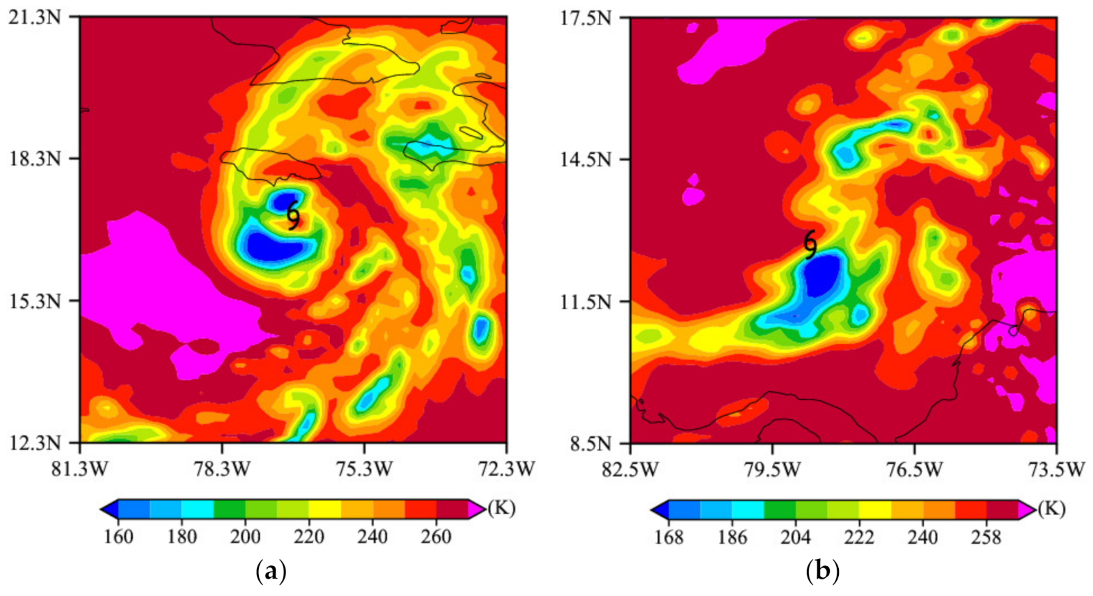
In order to conduct the proposed azimuthal spectral analysis, the first step is to determine an initial first-guess position of a targeted TC. Considering that there is usually a region of low brightness temperatures within the eyewall and the inner spiral rainbands, the first-guess position is determined by the minimum value of the average brightness temperature field encompassing a TC. Figure 3 shows two examples to illustrate the process of determining the first-guess position. Figure 3a shows the spatial distribution of the ATMS channel-18 brightness temperature field encompassing the hurricane Sandy at about 1438 UTC 24 October 2012. Figure 3c shows the averaged brightness temperature distributions at a 1.5° × 1.5° grid resolution. The grid point with the minimum brightness temperatures is indicated by the black cross symbol. We then move the same 1.5° × 1.5° grid resolution in the eastward and northward by 0.75°. Another point of the minimum brightness temperature is at the shifting grid mesh, which is indicated by grey cross symbol. The two averaging grid meshes are used to avoid the situation where the low brightness temperature region caused by the hurricane eyewall appears among the coarse grid points. The two positions are located at (−76.8° W, 16.8° N) and (−77.55° W, 16.05° N), respectively. The first-guess position is defined as the middle point between the two positions, which in this case is located at (−77.175° W, 16.425° N). Figure 3b shows the brightness temperature distribution at about 1756 UTC 22 October 2012 when Sandy’s eye is not apparent. Figure 3d shows that the first-guess position is similarly determined. The first-guess positions of Hurricane Sandy and Isaac such determined during their entire lifespans are shown in Section 4 and Section 5.

An example is given to illustrate the process of TC center positioning by the azimuthal spectral analysis. The azimuthal spectral analysis method is performed twice to find the TC center in the domain of the tryout centers with a coarse resolution of 0.15° × 0.15° for the first and a higher resolution of 0.05° × 0.05° for the second estimate. The first coarse resolution (0.15° × 0.15°) allows for a large domain of the tryout centers for finding a first estimate of the TC center, which is important if the initial first-guess position is poorly determined. The second fine resolution (0.05° × 0.05°) can determine the TC center from the tryout centers in a smaller domain centered at the first estimate. 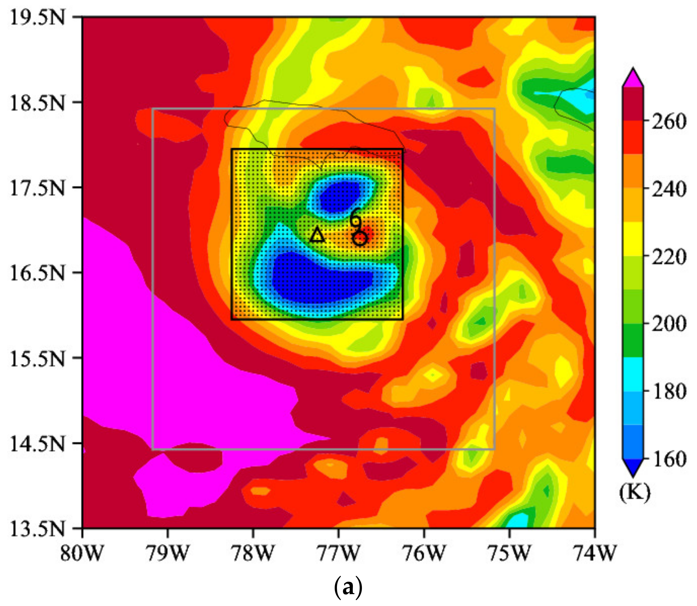Figure 4a shows the spatial distribution of the brightness temperature field with an interpolation resolution of 0.15° × 0.15° measured by the ATMS channel 18 at 1438 UTC 24 October 2012 and the tryout centers (all symbols in Figure 4a) in a 4° × 4° square area centered on the first-guess position indicated by the black cross. A set of azimuthal spectral analysis centered at different tryout centers is then carried out on the brightness temperature field. Figure 4b shows the variations of azimuthal wavenumber-0 amplitudes with a radial distance ranging from 30 km to 360 km from different tryout centers. The rules for determining the largest symmetric component are as follows: (1) the wavenumber-0 amplitude at the 30-km (or 360-km) radial distance of the azimuthal spectral analysis is greater than the average of wavenumber-0 amplitudes at the 30-km (or 360-km) radial distance from all tryout centers; (2) the value of wavenumber-0 amplitudes averaged from 30-km to 360-km radial distances is the largest. These rules are based on a hypothesis that the closer the tryout center is to the real TC center, the larger the wavenumber-0 amplitude. We can see that the largest symmetric component determined by series rules, indicated by the curve with triangle symbols in Figure 4b, is higher than those centered on the best track position, the guess position, and all other tryout centers. The tryout center corresponding to the largest symmetric component in Figure 4b is indicated by the triangle in Figure 4a, which is about 50 km away from the best track.

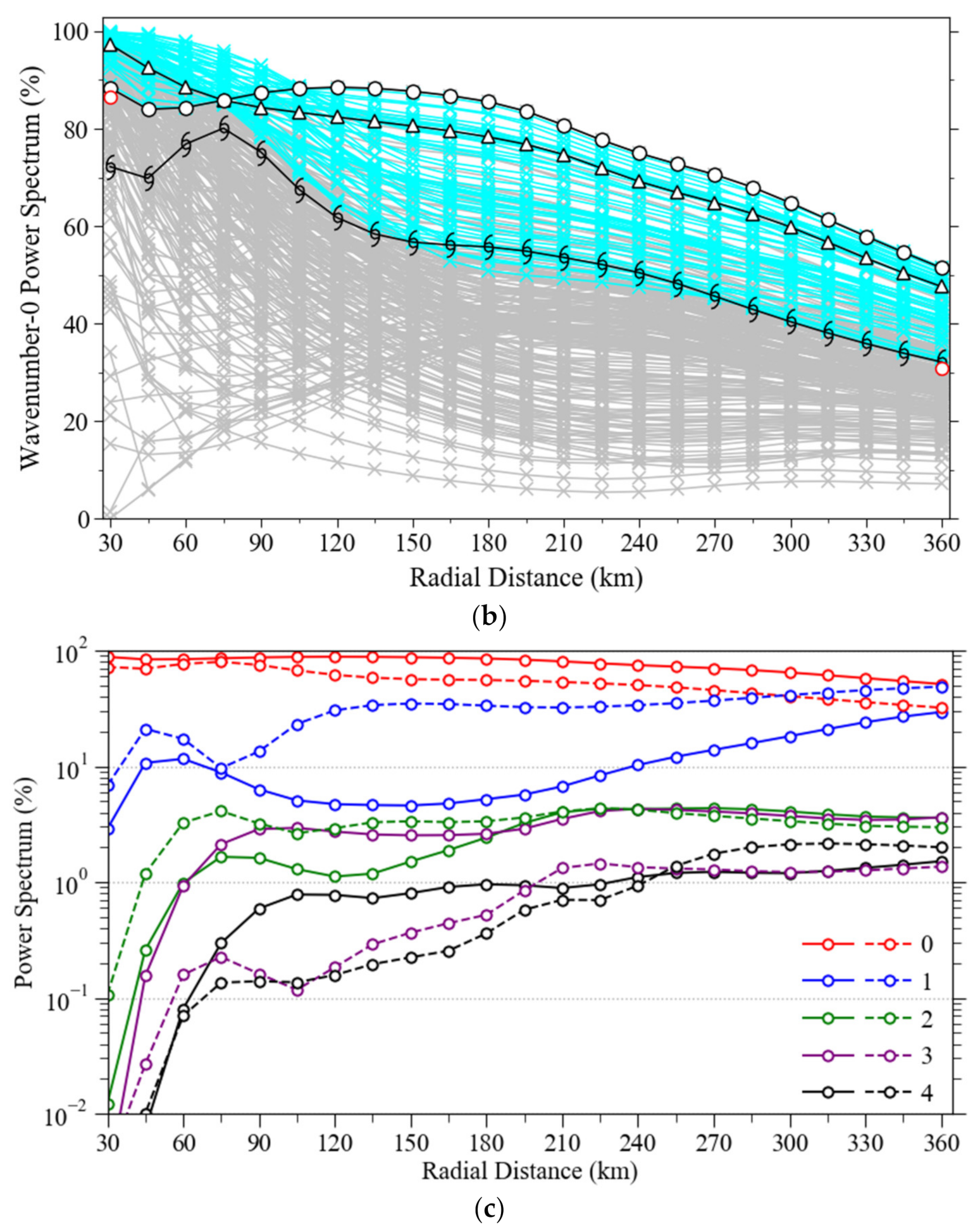
To refine the TC center position further, the domain of the tryout centers (black dots in Figure 5a) with a higher resolution of 0.05° × 0.05° is used. The 2° × 2° square area within which to search for the TC center is centered at the center position determined by the first step. Figure 5b shows the radial variations of azimuthal wavenumber-0 amplitudes centered at different tryout centers. The largest symmetric component is indicated by the curve with circles. Its wavenumber-0 component is larger than that centered on other tryout centers as well as the first-step-determined center and the best track center. Figure 5a shows that the center determined by the largest symmetric component is closest to the location of the warm core and deviates only slightly from the best track. Therefore, the domain of the tryout centers with a resolution of 0.05° × 0.05° leads to a more accurate TC center-positioning result than the first-step azimuthal spectral analysis.

There are still a few points that need further explanation. The first rule for determining the largest symmetric component is set to avoid the situations where the significant symmetric component at some radial distance arises from some local symmetric structures rather than the whole pattern of the TC, such as the two cases indicated by the purple color in Figure 4b. The wavenumber-0 amplitudes of the two cases account for less than 90% within 75 km and are significantly lower than that of the largest symmetric component. However, their wavenumber-0 amplitudes are slightly higher than those of the largest symmetric component between 90 and 270 km. For the situations indicated by the cyan color in Figure 4b, the wavenumber-0 amplitudes of them are higher than those of the largest symmetric component within a small radial distance (about 90–135 km) but significantly lower than those outside 135 km. In addition, it is worth noting that the azimuthal spectral analysis was carried out within radial distances from 30 to 360 km. Close to the TC center (less than 30 km), there are very little data for the azimuthal spectral analysis. In general, storm structure is more asymmetric in the outer region than in the inner core region. The strong asymmetric outer spiral rainbands are usually distributed in the periphery 500 km away from the TC center [26,27]. The outermost radius is empirically set to 360 km. As shown in Figure 4b and Figure 5b, the wavenumber-0 amplitudes remain much larger than those of higher wavenumbers within the 360-km radial distances.

Figure 5c shows the radial variations of wavenumbers 0–4 amplitude percentages from the ATMS-determined center (solid curves) and the best track (dashed lines). It is seen that, for the ATMS-determined center, the wavenumber-0 amplitude proportions are more than 80% within 210 km and then decrease slowly and finally account for about 50% at the 360-km radial distance. The wavenumber-0 amplitudes with the best track as the center of the azimuthal spectral analysis are smaller. The wavenumber-0 amplitudes for the ATMS-determined center in Figure 5c always account for the largest proportion of all wavenumbers’ amplitudes within 30–360-km radial distances, suggesting that the symmetric component dominates the entire pattern of the TC.

The TC center-positioning algorithm proposed in this study is different from that of [13]. In [13], an initial first-guess TC center position was determined by an extrapolation of the best track positions in the past 12 h; the ARCHER’s spiral centering method was employed to produce a modified TC center position from the first-guess position; and the azimuthal spectral analysis was merely used for eliminating impacts of small-scale cloud and water vapor disturbances, which makes a slight modification to the ARCHER-determined center position. In this study, an initial first-guess TC position is determined without using the best track data. The TC center position is solely determined by the azimuthal spectral analysis without employing any parts of the ARCHER algorithm.

4. The Center-Positioning Results of Hurricane Sandy

Figure 6a shows the track of Hurricane Sandy determined by the azimuthal spectral analysis method using the brightness temperature observations of ATMS channel 18 and MHS channel 5 as well as the NHC best track from 1800 UTC 21 October to 1200 UTC 31 October 2012. It is seen that the two tracks are quite close to each other. Figure 6b shows the track differences of ATMS- and MHS-determined TC centers from the best track after the first and second steps of the azimuthal spectral analysis method. We can see that the TC center-positioning differences after the second step are generally smaller than those of the first step during the lifetime of Sandy. The mean track error is about 35.8 km. Most of the TC center-fixing differences are lower than the average value when hurricane intensity is the highest during 1800 UTC 24 October and 1800 UTC 29 October 2012, and higher than the average value when hurricane intensity is relatively weak.

It is of interest to compare the ATMS- and MHS-determined TC centers in this study and the ATMS channel 22-determined TC centers [13]. The TC center-positioning results of them for Hurricane Sandy are shown in Figure 7. The two tracks determined by two different methods are basically consistent with each other and close to the best track (Figure 7a). Figure 7b shows the temporal variations of the TC center-positioning differences of ATMS channel 18 and MHS channel 5 and ATMS channel 22 for Hurricane Sandy. The mean difference determined by the ATMS channel 18 (35.8 km) used in this study is smaller than that of the ATMS channel 22 (43.6 km) [13]. One of the reasons for the better accuracy of using the ATMS channel 18 is the lower peak of the weighting function of the ATMS channel 18 (~800 hPa) than that of the ATMS channel 22 (~300 hPa), which allows for the ATMS channel 18 to reflect the water vapor structures better in the lower troposphere than the ATMS channel 22.

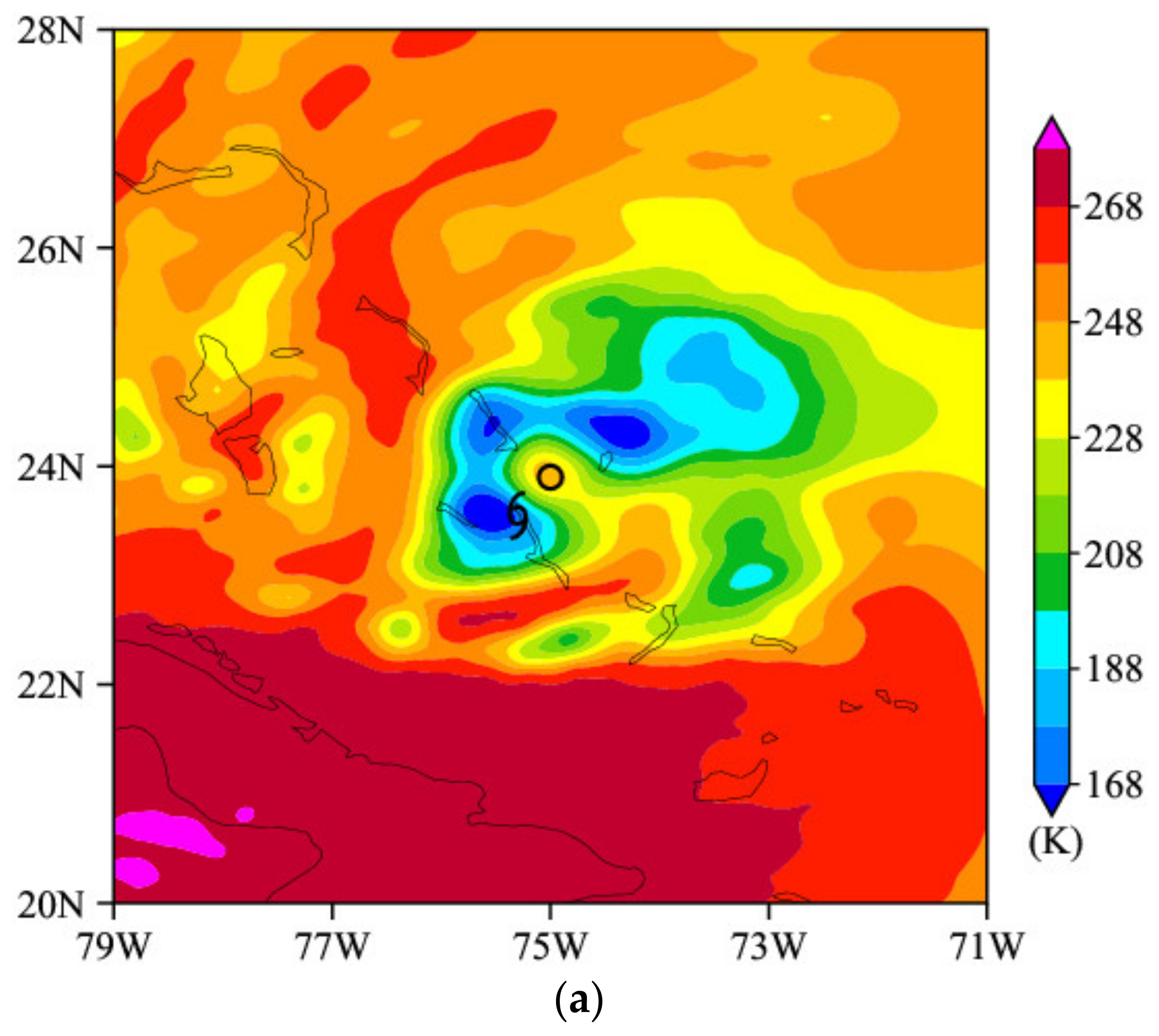
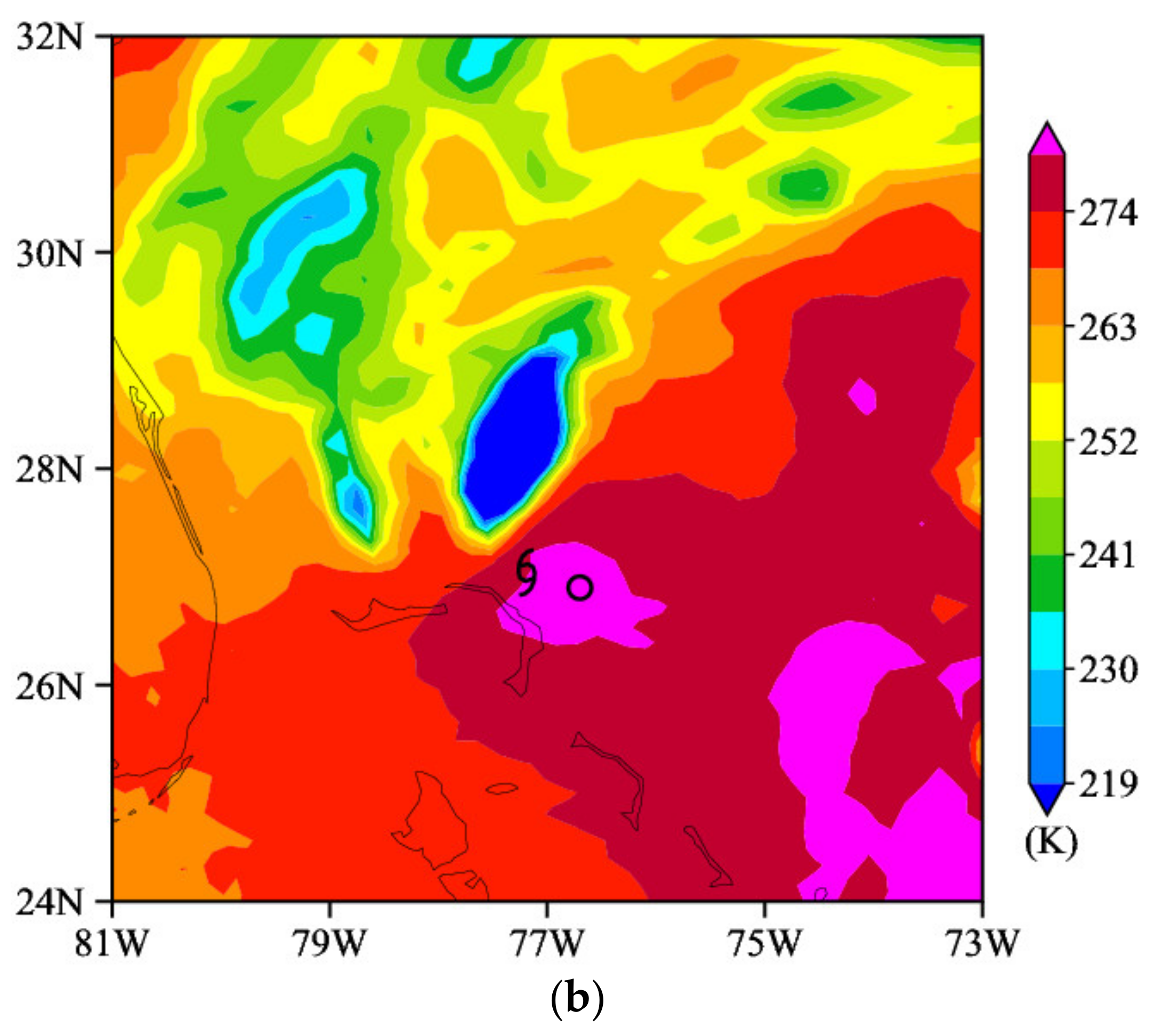
It is worth noting that, although the hurricane intensity is high at 1844 UTC 25 October and 1828 UTC 26 October 2012, the TC center-positioning errors at these two observing times are still slightly large (Figure 6b). We seek for possible causes of the relatively large positioning differences from the best track. Figure 8a shows the spatial distribution of ATMS channel-18 brightness temperature observation at 1844 UTC 25 October 2012. It is seen that the ATMS channel 18-determined TC center by the azimuthal spectral analysis method is just at the location of the maximum brightness temperature observation, which deviates from the best track by about 60 km. In other words, the ATMS-determined center is closer to the location of TC warm core, which reflects more of the TC center in the upper troposphere and may be different from the TC center near the surface which the best track determines.

Figure 8b shows the spatial distribution of ATMS channel-18 brightness temperature observation, the ATMS-determined TC center, and best track at 1828 UTC 26 October 2012. Compared with the TC case shown in Figure 8a, there was a larger positioning uncertainty in this case, because there was no obvious TC warm core or a spiral center to determine the optimal location of the TC center intuitively. In order to reveal the characteristics of the symmetric or asymmetric structures of the TC further, an azimuthal spectral analysis was carried out on both the brightness temperature fields shown in Figure 8a,b. Figure 9a shows the radial variations of wavenumbers 0–4 components centered at the ATMS-determined center (solid lines) and the best track (dashed lines) in the brightness temperature field containing a clear eye and obvious spiral rain bands shown in Figure 8a. It is seen that, for the ATMS-determined center that is close to the location of the eye, the wavenumber-0 amplitude always accounts for the largest proportion (over 50%) of all wavenumbers’ amplitudes within a 30–360-km radial distance, which indicates that the symmetric component dominates the whole pattern of the TC within the 360-km radial distances. For the best track, the wavenumber-0 amplitude is about 40% and larger than that of wavenumber 1 within a 30–225-km radial distance. However, the wavenumber-1 amplitude exceeds the wavenumber-0 amplitude beyond the 225-km radial distances and keeps a stable value of about 50%. The surpassing of wavenumber-1 amplitude to wavenumber-0 amplitude indicates that the asymmetric component dominates the entire pattern of the TC at the corresponding radial distance. Figure 9b shows the radial variations of wavenumbers 0–4 components of the brightness temperature field shown in Figure 8b. For the ATMS-determined center, the wavenumber-0 amplitude accounts for more than 90% within 30–90 km and then decreases rapidly with the radial distance after 90 km, and finally gradually keeps stable at about 5%. The wavenumber-1 amplitude exceeds wavenumber 0 when radial distances are greater than 135 km and gradually keeps a stable value of about 40%. The wavenumber-2 amplitude exceeds wavenumber 0 beyond the 150-km radial distance and keeps a stable value of about 20%. Similarly, for the best track, the amplitude of wavenumber 1 exceeds that of wavenumber 0 beyond the 75-km radial distance and remains a constant value of about 50%. Obviously, the TC at this time is strongly asymmetric within the 360-km radial distance, which makes the azimuthal spectral analysis method proposed in this study less appropriate for determining TC centers. Therefore, a largely asymmetry of the TC structure seems to increase the positioning uncertainty of the ATMS- and MHS-determined TC center positions, causing a large difference between our results and the best track.

In conclusion, the azimuthal spectral analysis method for determining TC centers is effective when the symmetric component dominates the whole pattern of the TC, but the positioning uncertainty would increase if a TC was significantly asymmetric. If the structure of a TC is significantly asymmetric with respect to the TC center, it may be necessary to take into consideration more wavenumbers for determining the TC center positions, which requires further investigation.

Figure 10 shows the brightness temperature fields encompassing Hurricane Sandy along the track determined by the ATMS and MHS at nine selected observing times. It provides the structural evolution of Sandy along its track. Sandy began to strengthen at a faster rate on 23 October, with the spiral rain band becoming more prominent east and south of the center. Sandy became a hurricane at 1200 UTC 24 October while centered near the Kingston with an apparent hurricane eye in the microwave observations. After Sandy moved to the south of Cuba over the warm waters, it rapidly intensified to a major hurricane with a circularly organized deep convection surrounding the hurricane eye at 0556 UTC 25 October. Sandy began to weaken after making landfall in Cuba and then weakened more quickly on late 25 October. After Sandy moved northeastward away from the Bahamas on 27 October, it weakened to a tropical storm and had greatly increased size. The average radii of winds (such as the 34- and 64-kt winds) measured by the NHC best track roughly doubled since the time of landfall in Cuba. Sandy regained hurricane strength at 0208 UTC 28 October, while the radius of maximum wind was very large (over 250 km). Sandy took on a more tropical appearance with hints of an eye near its center and a spiral rain band belt on the periphery at 1455 UTC 28 October. Sandy turned toward the northwest later on 29 October, weakened, and gradually lost tropical characteristics.

5. The Center-Positioning Results of Hurricane Isaac

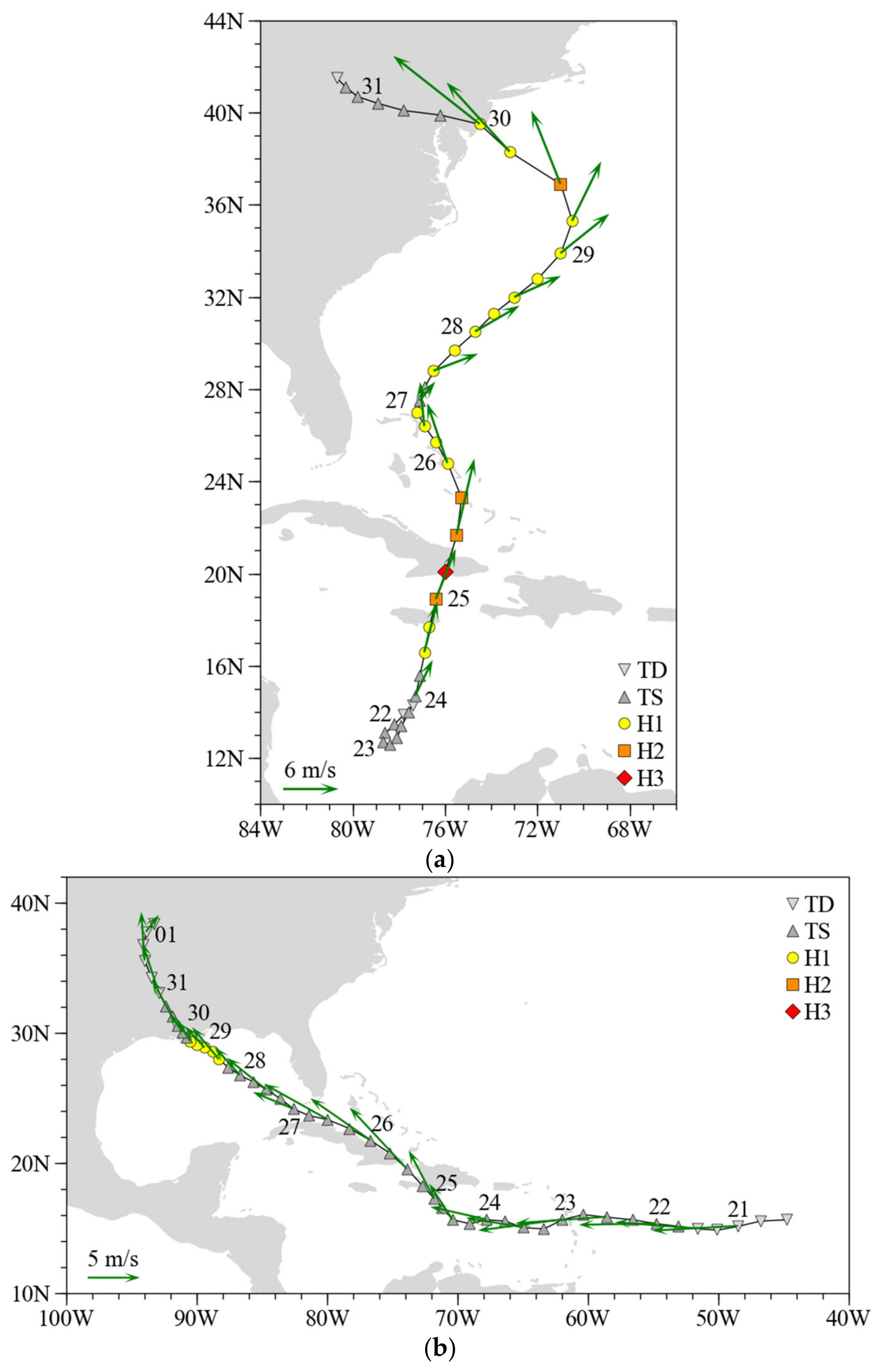
Different from Hurricane Sandy with an abnormal track over the Atlantic Ocean (Figure 11a), Hurricane Isaac has a typical track initially moving westward and then continuously moving northwestward (Figure 11b). The motions of both hurricanes are highly correlated with the steering flow. Figure 12 shows potential vorticity and geopotential height at 200 hPa at eight selected times during the lifetime of Isaac. Isaac moved quickly westward before 24 August caused by a strong subtropical ridge over the western Atlantic and turned northwestward at about 1200 UTC 24 August. After that, Isaac moved northwest led by the steering flow until it made landfall in Louisiana on 29 August. Isaac gradually weakened after it moved inland and turned northward later on 31 August. Unlike Sandy, Isaac is less affected by a large-scale weather system, such as a trough or ridge, which gives it a typical northwestward track in the Northern Hemisphere.

The same azimuthal spectral analysis method was also applied to locate the TC centers of Hurricane Isaac using the brightness temperature observations of ATMS channel 18 and MHS channel 5. Figure 13a shows the ATMS- or MHS-determined center positions and the best track of Isaac from 1717 UTC 21 August to 0819 UTC 30 August 2012. It is seen that there are obvious differences between the two tracks before 24 August, and the differences become very small after that. Figure 13b shows the deviations of ATMS- or MHS-determined TC center positions from the best track after the first and second step of the azimuthal spectral analysis method. The TC center-fixing differences after the second step are generally smaller than that of the first step during the lifetime of Isaac, which is consistent with Hurricane Sandy. In addition, the track errors of the ATMS channel 18- and the MHS channel 5-determined TC centers in this study and the ATMS channel 22-determined TC centers [13] were compared in Figure 13b. The mean track differences from both methods are quite close (about 31.3 km versus 31.6 km). Besides, the TC center-positioning differences are relatively large on average when the hurricane intensity is relatively weak before 1200 UTC 24 August 2012, and smaller when hurricane intensity is high during 1200 UTC 24 August and 1800 UTC 29 August 2012. The results of TC center-positioning differences of Hurricane Isaac and Sandy indicate that the positioning error of the azimuthal spectral analysis method is affected by the intensity of a TC. In general, the TC eye is clearly seen, and the spiral structure is more symmetric when the TC intensity is high, which contributes to a strong symmetric component and benefits the determination of the TC center by the azimuthal spectral analysis method. However, when a TC is weak, the TC structure is generally discrete, which leads to a weak symmetric component and thus a slightly larger positioning uncertainty for the azimuthal spectral analysis method.

6. Validation of the TC Centering Algorithm for Tropical Storms and Hurricanes over Atlantic and Pacific Oceans in 2019

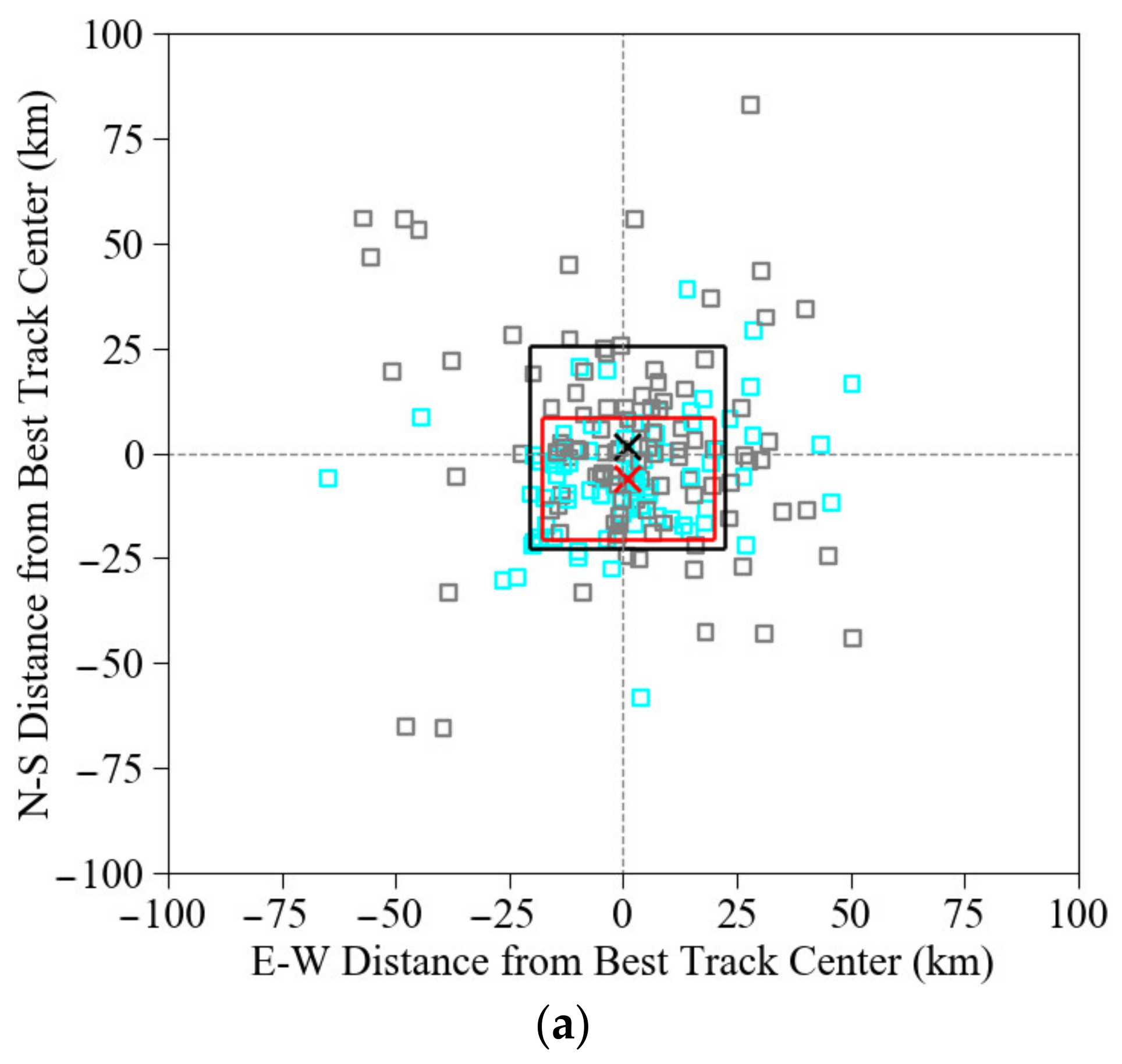
In order to assess whether the proposed method is, in general, applicable to other tropical cyclone cases for a large validation sample, the proposed TC centering algorithm is applied to all tropical storms and hurricanes over the Atlantic and Pacific oceans in 2019. There were 180 cases over the Atlantic ocean and 468 cases over the Pacific ocean for which the observations of ATMS onboard S-NPP satellite and the MHS onboard MetOp-A satellite were collected, and the single ATMS and MHS water vapor sounding channel algorithm was applied.

Deviations of the TC center positions determined by the proposed azimuthal spectral analysis method from the best track center are less than 100 km for individual cases, and the standard deviations in the east-west or north-south directions are less than 25 km (Figure 14). Figure 15 shows the variations of the number of tropical storms and hurricanes in 2019 with respect to the distances between the best track and the TC centers determined by the proposed algorithm using ATMS and MHS single channel observations. For a total of 648 cases in 2019, the distances of the TC centers between our results and the best track are less than 40 km (30 km) for more than 84% (72%). The cases with smaller position differences are much more than those with large position differences. The standard deviations for tropical storms over both the Atlantic or Pacific oceans are relatively larger than those for hurricanes. The root-mean-square differences of the TC center positions determined by the proposed azimuthal spectral analysis for a single water vapor sounding channel are 33.81, 26.2, and 30.65 km for tropical storms only, hurricanes only, and all cases, respectively (

Table 1. The root-mean-square of the distances (km) of TC center positions between our results and the best track for tropical storms and hurricanes over Atlantic and Pacific oceans in 2019. The case numbers are indicated in the bracket.

Ocean Basin	All Cases	Tropical Storms	Hurricanes
Atlantic	31.63 (180)	35.45 (104)	25.50 (76)
Pacific	30.26 (468)	33.13 (255)	26.44 (213)
Atlantic and Pacific	30.65 (648)	33.81 (359)	26.20 (289)

). It is worth noting that the center position of the best track usually refers to the location of minimum near-surface wind or minimum sea-level pressure, which is obtained by combining reconnaissance aircraft penetration, satellite, radar, and synoptic data. Therefore, the TC center position determined from a single satellite channel in this study could be different from the best track definition. The latter is used as reference data for validating our results.

7. Discussion

The azimuthal spectral analysis method for locating the center of a tropical storm or hurricane objectively by using single channel microwave satellite observations of brightness temperature has been proved to be feasible. This method offers a real-time capability for vortex initialization in operational hurricane forecasts. However, the TC center-fixing technique requires a TC with a tropical storm level or above and is based on the premise that the whole pattern of a TC is dominated by the symmetric component. The center positioning of a tropical depression and the scenario where the asymmetric component dominates the whole pattern of a TC needs further study in the future. Besides, compared with the microwave observations from a polar-orbiting satellite, the infrared and visible observations from a geostationary satellite have a higher spatial and temporal resolution. In the future, we will apply the azimuthal spectral analysis method to the geostationary visible and infrared observations to locate TC centers.

8. Conclusions

The microwave humidity sounding channels of the Advanced Technology Microwave Sounder and the Microwave Humidity Sounder are capable of probing the atmospheric moisture and cloud distributions in the troposphere. They are especially important for TC studies. An azimuthal spectral analysis method suited for objectively determining the TC center in real time using single-channel brightness temperature observations from the Advanced Technology Microwave Sounder and the Microwave Humidity Sounder is developed and tested in this study. This TC center-fixing technique locates the TC center by comparing the symmetric components centered at different tryout centers in the brightness temperature field encompassing a TC. The center that gives the largest symmetric component would be regarded as the final TC center. Hurricane Sandy and Isaac, which have different track and intensity characteristics, are first used as examples to show the performance of the TC center-fixing technique. Compared with the best track, the TC center-fixing technique achieves a root-mean-square difference of about 47.3 and 34.3 km for Sandy and Isaac, respectively. By examining the structural evolution of Hurricane Sandy in the microwave humidity sounding observations, we found that there would be a slightly larger positioning uncertainty when an asymmetric component dominates the whole pattern of a TC. To determine the TC center more accurately, more wavenumbers perhaps should be taken into account when a TC is significantly asymmetric. This is the focus of our future research. Finally, all tropical storms and hurricanes over the Northern Atlantic and Western Pacific oceans in 2019 are used to validate the TC center-positioning algorithm. The root-mean-square center-positioning errors of tropical storms and hurricanes are 33.81 and 26.20 km, respectively.

References

1. Chang, P.L.; Jou, B.J.-D.; Zhang, J. An algorithm for tracking eyes of tropical cyclones. Weather Forecast. 2009, 24, 245–261. [Google Scholar] [CrossRef]
2. Huang, X.; Peng, X.; Fei, J.; Cheng, X.; Ding, J.; Yu, D. Evaluation and error analysis of official tropical cyclone intensity forecasts during 2005–2018 for the Western North Pacific. J. Meteorol. Soc. Soc. Jpn. 2021, 99, 139–163. [Google Scholar] [CrossRef]
3. Velden, C.; Harper, B.; Wells, F.; Beven, J.L.; Zehr, R.; Olander, T.; Mayfield, M.; Guard, C.C.; Lander, M.; Edson, R.; et al. Supplement to: The Dvorak tropical cyclone intensity estimation technique: A satellite-based method that has endured for over 30 years. Bull. Am. Meteorol. Soc. 2006, 87, S6–S9. [Google Scholar] [CrossRef]
4. Olander, T.L.; Velden, C.S. The Advanced Dvorak Technique (ADT)—Continued development of an objective scheme to estimate tropical cyclone intensity using geostationary infrared satellite imagery. Weather Forecast. 2007, 22, 287–298. [Google Scholar] [CrossRef]
5. Dvorak, V.F. Tropical Cyclone Intensity Analysis Using Satellite Data; NOAA Tech. Rep. 11; NOAA/NESDIS: Washington, DC, USA, 1984; p. 45. [Google Scholar]
6. Dvorak, V.F. Tropical Clouds and Cloud Systems Observed in Satellite Imagery: Tropical Cyclones; Workbook Vol. 2; NOAA/NESDIS: Washington, DC, USA, 1995; p. 359. [Google Scholar]
7. Velden, C.S.; Olander, T.L.; Zehr, R.M. Development of an objective scheme to estimate tropical cyclone intensity from digital geostationary satellite infrared imagery. Weather Forecast. 1998, 13, 172–186. [Google Scholar] [CrossRef] [Green Version]
8. Wimmers, A.; Velden, C.S. Satellite-based center-fixing of TCs: New automated approaches. In Proceedings of the 26th Conference on Hurricanes and Tropical Meteorology, Miami, FL, USA, 3–7 May 2004; pp. 82–83. [Google Scholar]
9. Olander, T.L.; Velden, C.S.; Turk, M.A. Development of the advanced objective Dvorak technique (AODT)—Current progress and future directions. In Proceedings of the 25th Conference on Hurricanes and Tropical Meteorology, San Diego, CA, USA, 28 April 2002; pp. 585–586. [Google Scholar]
10. Olander, T.; Velden, C.S.; Kossin, J. The Advanced Objective Dvorak technique (AODT): Latest upgrades and future directions. In Proceedings of the 26th Conference on Hurricanes and Tropical Meteorology, Miami, FL, USA, 3–7 May 2004; pp. 294–295. [Google Scholar]
11. Wimmers, A.J.; Velden, C.S. Objectively determining the rotational center of tropical cyclones in passive microwave satellite imagery. J. Appl. Meteor. Climatol. 2010, 49, 2013–2034. [Google Scholar] [CrossRef]
12. Wimmers, A.J.; Velden, C.S. Advancements in objective multi-satellite tropical cyclone center fixing. J. Appl. Meteor. Climatol. 2016, 55, 197–212. [Google Scholar] [CrossRef]
13. Hu, Y.; Zou, X. Comparison of tropical cyclone center positions determined from satellite observations at infrared and microwave frequencies. J. Atmos. Ocean. Technol. 2020, 37, 2101–2115. [Google Scholar] [CrossRef]
14. Weng, F.; Zou, X.; Wang, X.; Yang, S.; Goldberg, M.D. Introduction to Suomi National Polar-orbiting Partnership Advanced Technology Microwave Sounder for numerical weather prediction and tropical cyclone applications. J. Geophys. Res. Atmos. 2012, 117, 1–14. [Google Scholar] [CrossRef]
15. Wood, V.T. A technique for detecting a tropical cyclone center using a Doppler radar. J. Atmos. Ocean. Technol. 1994, 11, 1207–1216. [Google Scholar] [CrossRef] [Green Version]
16. Wong, K.Y.; Yip, C.L.; Li, P.W.; Tsang, W.W. Automatic template matching method for tropical cyclone eye fix. In Proceedings of the 17th International conference Pattern Recognition (ICPR’04), Cambridge, UK, 26 August 2004; pp. 650–653. [Google Scholar]
17. Wong, K.Y.; Yip, C.L.; Li, P.W. A novel algorithm for automatic tropical cyclone eye fix using Doppler radar data. Meteor. Appl. 2007, 14, 49–59. [Google Scholar] [CrossRef]
18. Wong, K.Y.; Yip, C.L.; Li, P.W. Automatic tropical cyclone eye fix using genetic algorithm. Expert Syst. Appl. 2008, 34, 643–656. [Google Scholar] [CrossRef]
19. Wong, K.Y.; Yip, C.L. Identifying centers of circulating and spiraling vector field patterns and its applications. Pattern Recognit. 2009, 42, 1371–1387. [Google Scholar] [CrossRef]
20. Landsea, C.W.; Franklin, J.L. Atlantic Hurricane database uncertainty and presentation of a new database format. Mon. Weather Rev. 2013, 141, 3576–3592. [Google Scholar] [CrossRef]
21. Velden, C.S.; Leslie, L.M. The Basic Relationship between Tropical Cyclone Intensity and the Depth of the Environmental Steering Layer in the Australian Region. Weather Forecast. 1991, 6, 244–253. [Google Scholar] [CrossRef] [Green Version]
22. Wu, Y.; Zou, X. Numerical test of a simple approach for using TOMS total ozone data in hurricane environment. Q. J. R. Meteorol. Soc. 2008, 134, 1397–1408. [Google Scholar] [CrossRef]
23. Corbosiero, K.L.; Molinari, J.; Aiyyer, A.R.; Black, M.L. The Structure and Evolution of Hurricane Elena (1985). Part II: Convective Asymmetries and Evidence for Vortex Rossby Waves. Mon. Weather Rev. 2006, 134, 3073–3091. [Google Scholar] [CrossRef]
24. Tian, X.; Zou, X. A comprehensive 4D-Var vortex initialization using a nonhydrostatic axisymmetric TC model with convection accounted for. Tellus A Dyn. Meteorol. Oceanogr. 2019, 71, 1653138. [Google Scholar] [CrossRef] [Green Version]
25. Zou, X.; Wu, Y.; Ray, P.S. Verification of a high-resolution model forecast using airborne Doppler radar analysis during the rapid intensification of Hurricane Guillermo. J. Appl. Meteor. Climatol. 2010, 49, 807–820. [Google Scholar] [CrossRef]
26. Guinn, T.A.; Schubert, W.H. Hurricane spiral bands. J. Atmos. Sci. 1993, 50, 3380–3403. [Google Scholar] [CrossRef] [Green Version]
27. Houze, R.A., Jr. Clouds in tropical cyclones. Mon. Weather Rev. 2010, 138, 293–344. [Google Scholar] [CrossRef]
Figure 1. Temporal evolutions of (a) the best track, (b,c) the maximum sustained wind (m s1; open symbol), minimum central pressure (hPa; solid symbol) of (b) Hurricanes Sandy from 1800 UTC 21 to 1200 UTC 31 October 2012 and (c) Isaac from 1200 UTC 20 August to 0600 UTC 1 September 2012. Intensity category is indicated by different symbols and shading colors.
Remotesensing 13 02466 g001aRemotesensing 13 02466 g001b
Figure 2. Potential vorticity (color shading; 1 PVU = 10−6 K·m2 kg−1·s−1) and geopotential height (contour; unit: m) at 200 hPa from the ERA5 analysis valid at (a) 0000 UTC 24, (b) 0000 UTC 25, (c) 0000 UTC 26, (d) 1200 UTC 26, (e) 1200 UTC 27, (f) 0000 UTC 29, (g) 1200 UTC 29, and (h) 0000 UTC October 2012 for Hurricane Sandy whose center positions from best track are indicated by hurricane symbol. What is also indicated is the deep-layer mean wind (red arrow, the length of 6 m·s−1) calculated from the ERA5 winds within the 500-km radius of Sandy.
Remotesensing 13 02466 g002
Figure 3. Spatial distributions of (a,b) ATMS channel-18 brightness temperature observations (color shading) and (c,d) averaged brightness temperature at a 1.5° × 1.5° grid resolution for Hurricane Sandy at about 1438 UTC 24 (left panels) and 1756 UTC 22 (right panels) October 2012. The black and grey cross symbols indicate locations of the lowest averaged brightness temperature with a 0.75° eastward and northward shifting, and their middle point (red cross symbol) is defined as the first-guess position.
Remotesensing 13 02466 g003aRemotesensing 13 02466 g003b
Figure 4. (a) Spatial distribution of ATMS channel-18 brightness temperature observations (color shading) for Hurricane Sandy (Category 2, 44 m s−1) at about 1438 UTC 24 October 2012, the best track (hurricane symbol), the first-guess position (black cross), ATMS channel 18-determined center after the 1st step (black triangle). The grey box is 4.0° × 4.0°. (b) Radial variations of the azimuthal wavenumber-0 amplitude percentages (curves; %) with the grid points (black dots in (a)) as assumed TC centers. The cyan curves with crosses indicate those tryout centers for which the wavenumber-0 amplitudes are larger (smaller) than the center determined by the first azimuthal spectral analysis at small (larger) radial distances. The purple color is to indicate those tryout centers for which the wavenumber-0 amplitudes are smaller (larger) than the center determined by the first azimuthal spectral analysis at small (larger) radial distances. The means (red circle) of wavenumber-0 power spectrum at 30- and 360-km radial distances are indicated.
Remotesensing 13 02466 g004
Figure 5. (a,b) are same as Figure 4 except for using a domain of the tryout centers (black dots) with higher grid resolution of 0.05° × 0.05° to obtain a further refined TC center (black open circle) in the 2.0° × 2.0° black box. Note that the interval of tryout centers corresponding to the wavenumber-0 amplitude curves shown in (b) are set to be 0.25°. (c) Radial variations of wavenumbers 0–4 amplitude percentages (curves; %) with radial distance from ATMS determined Sandy’s center (solid curves) or the best track (dashed curves) at about 1438 UTC 24 October 2012.
Remotesensing 13 02466 g005aRemotesensing 13 02466 g005b
Figure 6. (a) ATMS channel 18 (cyan) or MHS channel 5 (blue) determined track, the first-guess position track (black line with crosses), and the best track (red) from 1800 UTC 21 October to 1200 UTC 31 October 2012. (b) Track errors of ATMS/MHS-determined TC centers after the first step (gray symbols) and the second step (blue for MHS and cyan for ATMS), and the maximum sustained wind (shading, unit: m s−1). The mean positioning error (dashed line) of ATMS/MHS-determined tracks for Sandy from 0652 UTC 22 October to 0104 UTC 31 October 2012 is 35.8 km.
Remotesensing 13 02466 g006aRemotesensing 13 02466 g006b
Figure 7. Same as Figure 6 except for (a) the ATMS channel 22-determined track (green) and (b) track errors of ATMS channel 22-determined TC centers (green). The mean position error (green dashed line) of ATMS channel 22-determined tracks for Sandy from 0652 UTC 22 October to 0104 UTC 31 October 2012 is 43.6 km.
Remotesensing 13 02466 g007aRemotesensing 13 02466 g007b
Figure 8. Spatial distributions of ATMS channel-18 brightness temperature observations (color shading) for Hurricane Sandy at about (a) 1844 UTC 25 October 2012 and (b) 1828 UTC 26 October 2012. The best track (hurricane symbol) and the ATMS channel 18-determined center by the azimuthal spectral analysis method (black circle) are also indicated.
Remotesensing 13 02466 g008aRemotesensing 13 02466 g008b
Figure 9. Radial Variations of wavenumbers 0–4 amplitude proportions (curves; %) to the total ten wavenumber amplitudes with radial distance from ATMS-determined Sandy’s center (solid curves) or the best track (dashed curves) at about (a) 1844 UTC 25 October 2012 and (b) 1828 UTC 26 October 2012.
Remotesensing 13 02466 g009
Figure 10. Spatial distributions of TB observations (color, 8° × 8° area) along the track of Hurricane Sandy (black symbols) at nine selected observing times.
Remotesensing 13 02466 g010
Figure 11. The steering flow vectors (green) along the best tracks of (a) Hurricane Sandy from 1800 UTC 21 October to 1200 UTC 31 October 2012 and (b) Hurricane Isaac from 1200 UTC 20 August to 0600 UTC 1 September 2012.
Remotesensing 13 02466 g011
Figure 12. Same as Figure 2 except for Hurricane Isaac from 1200 UTC 20 August to 0000 UTC 01 September 2012 (ah).
Remotesensing 13 02466 g012
Figure 13. (a) Same as Figure 6a and (b) same as Figure 7b except for Isaac from 1200 UTC 21 August to 1200 UTC 30 August 2012. The mean positioning errors of the ATMS channel 18 (or the MHS channel 5, black dashed line) and the ATMS channel 22 [13] (green dashed line) for Isaac from 1717 UTC 21 August to 0819 UTC 30 August 2012 are 31.3 and 31.6 km, respectively.
Remotesensing 13 02466 g013
Figure 14. Scatterplots (grey for tropical storms and cyan for hurricanes) of the deviations of the TC center positions from the best track in the east-west (E-W) and north-south (N-S) directions for (a) 180 TC cases over Atlantic ocean, (b) 468 cases over Pacific ocean, and (c) all cases in 2019. What are also indicated are the mean (cross symbol) and ± one standard deviation (square box) for tropical storms (black) and hurricanes (red). The E-W (N-S) standard deviations are 21.53 (24.15), 21.97 (24.85), and 21.86 (24.67) km for tropical storms, and 18.93 (14.51), 17.93 (18.30), and 18.32 (17.57) km for hurricanes in (a), (b), and (c), respectively.
Remotesensing 13 02466 g014aRemotesensing 13 02466 g014b
Figure 15. Variations in the number of TC cases with respect to the distances between the best track and the TC center positions determined by the proposed method using ATMS and MHS single channel observations for all tropical storms (hatched bar) ad hurricanes (solid bar) over Atlantic (cyan), Pacific (yellow) oceans, and the total (green) at 10-km interval.
Remotesensing 13 02466 g015