
A GNSS-IR Method for Retrieving Soil Moisture Content from Integrated Multi-Satellite Data That Accounts for the Impact of Vegetation Moisture Content

 ,
,  , ,
, ,  ,
,
Abstract
:1. Introduction
2. Materials and Methods
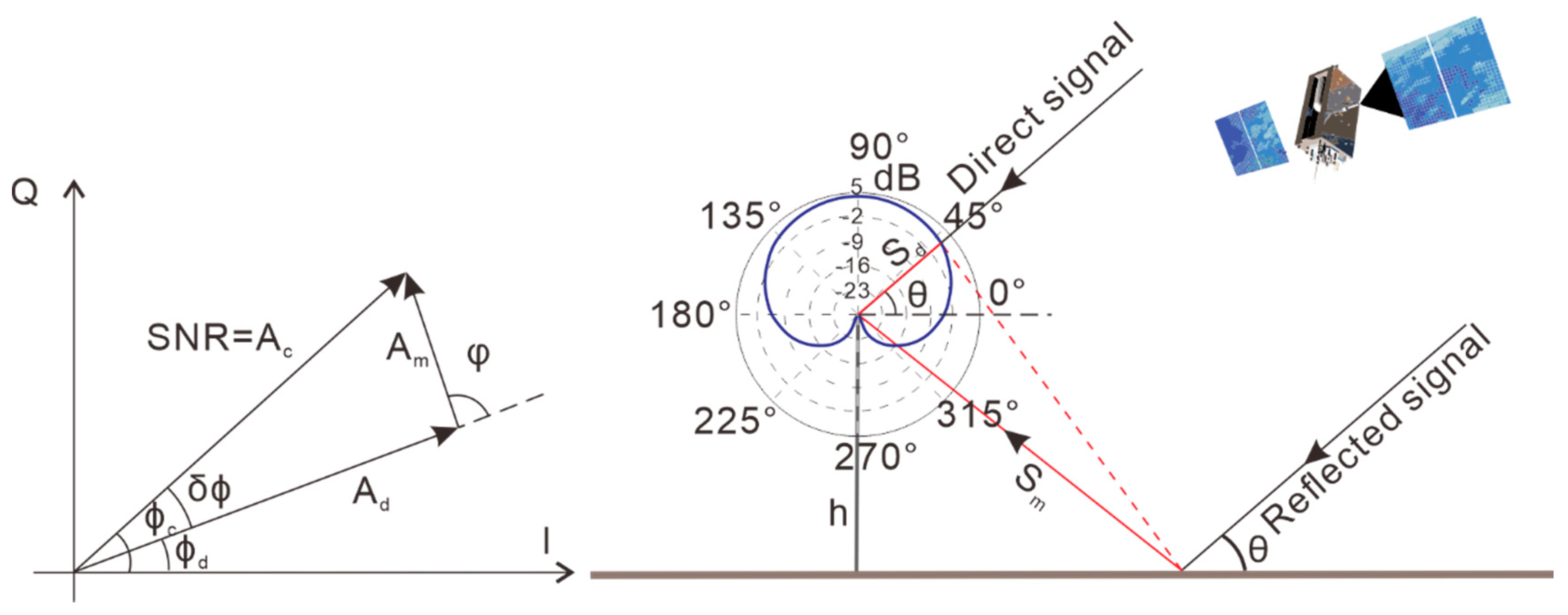
2.1. GNSS-IR SMC Retrieval Principle
2.2. Vegetation Error Correction Based on the Multipath Effect
2.3. MARS Model
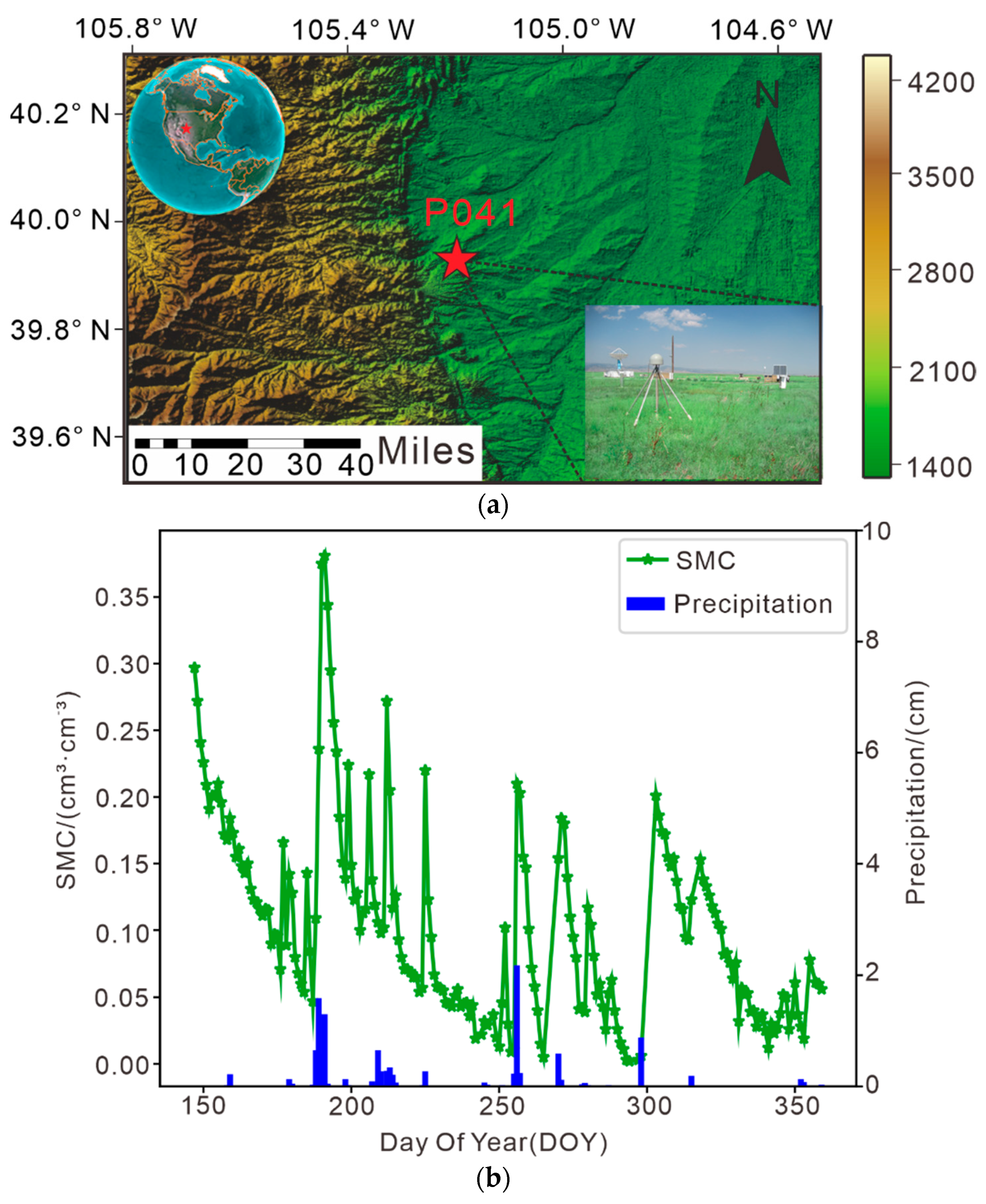
3. Data Sources
4. Experiment and Results
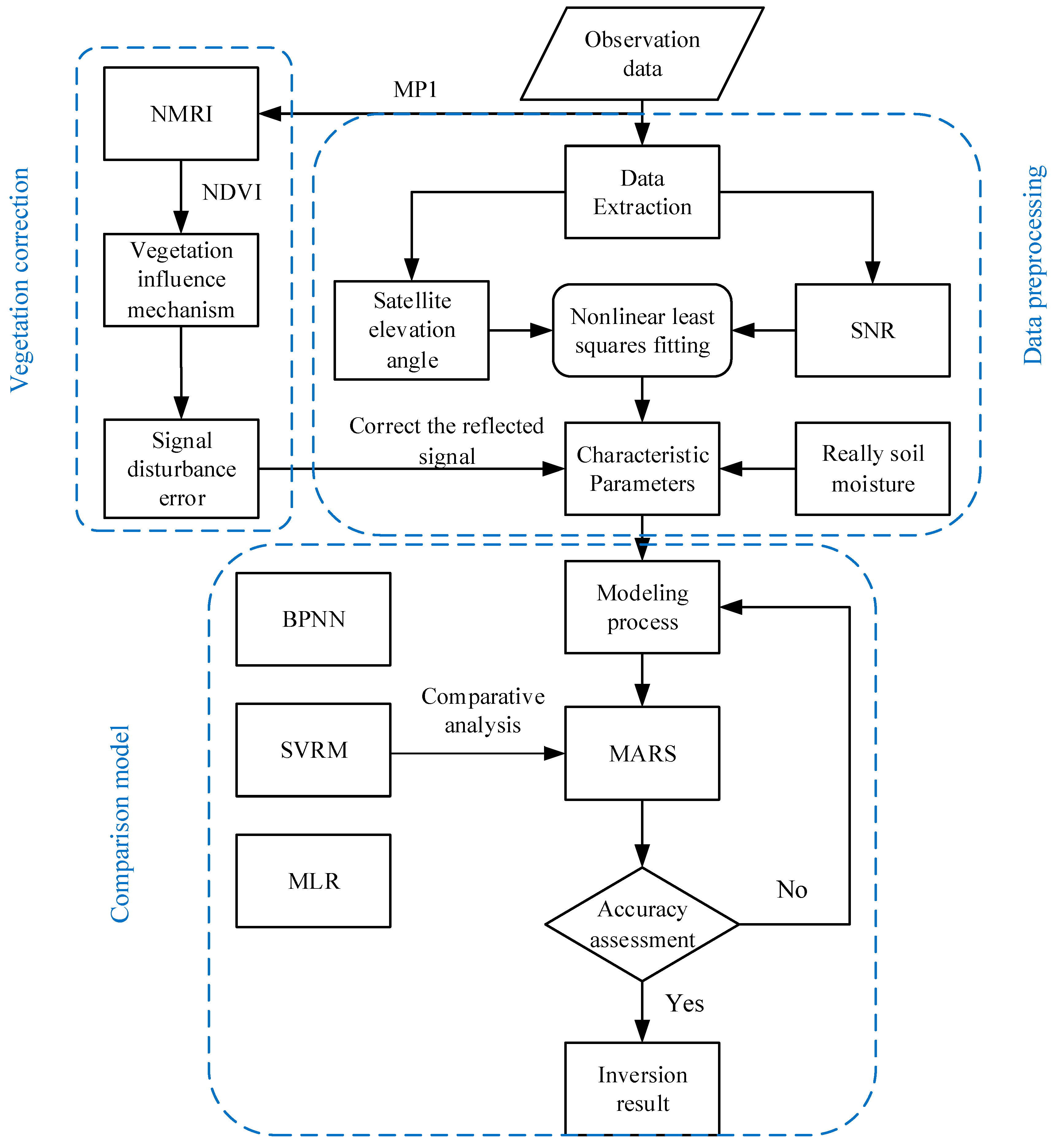
4.1. Experimental Technical Scheme
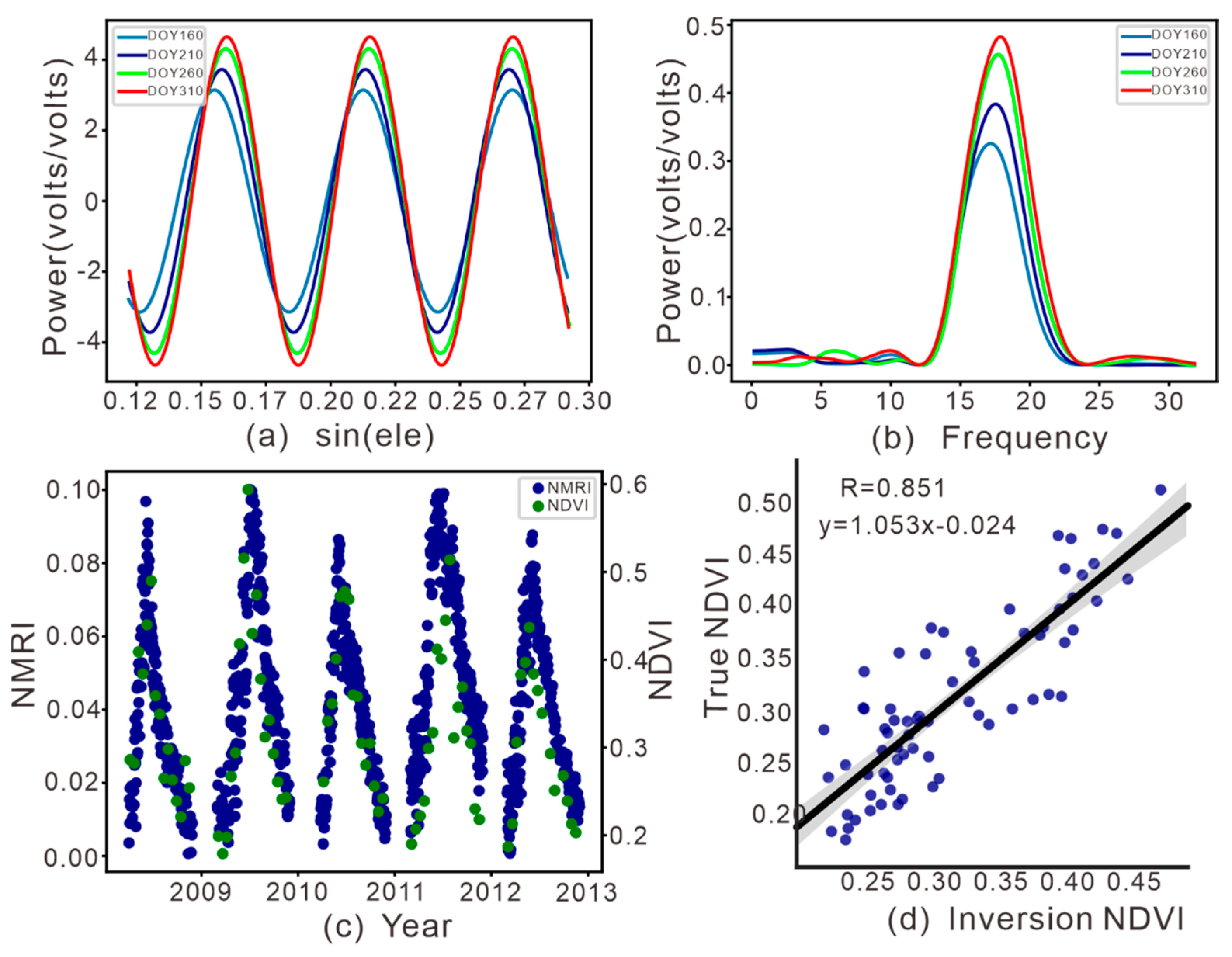
4.2. Reflected Signal Feature Parameter Extraction
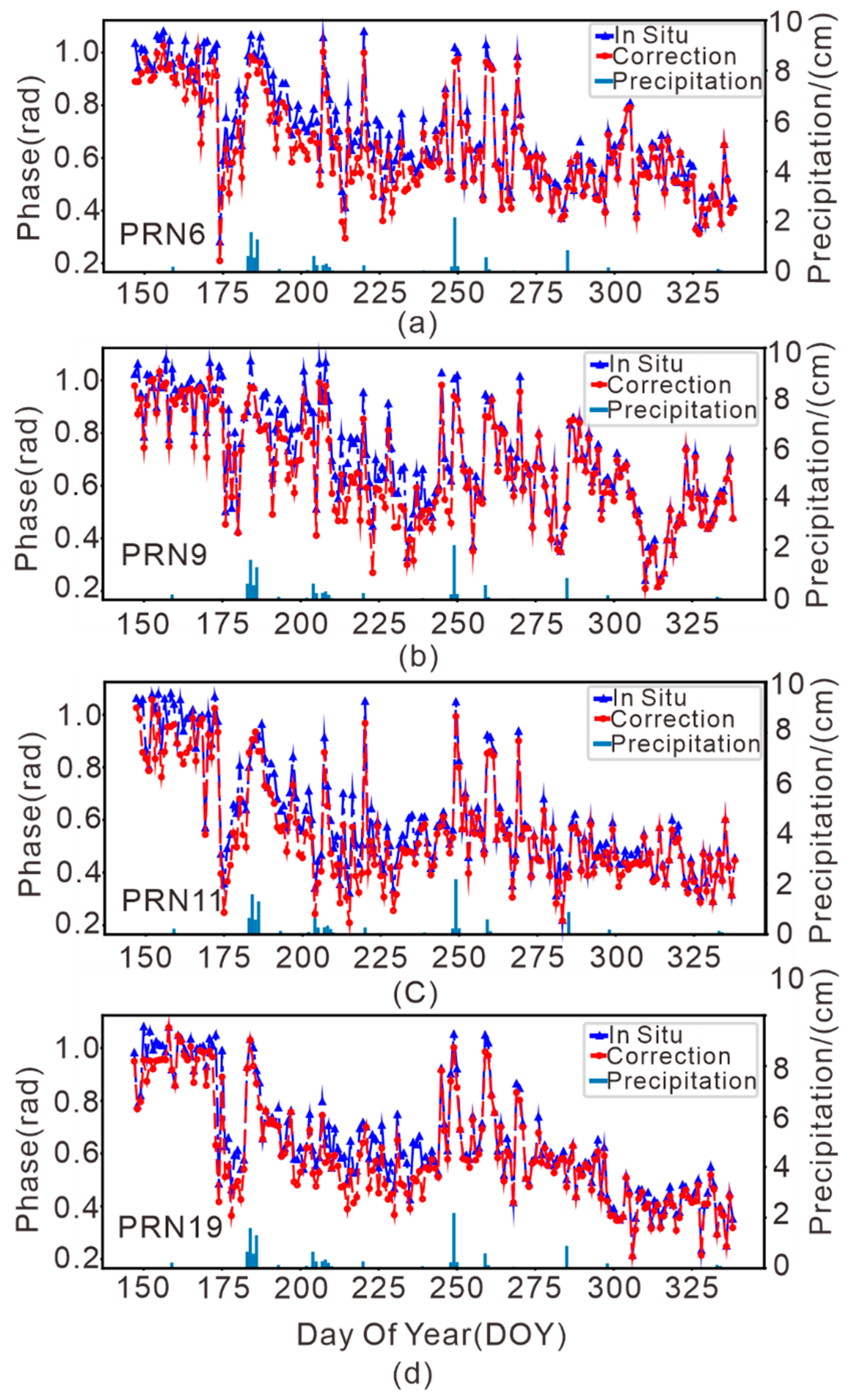
4.3. Vegetation Impact Correction
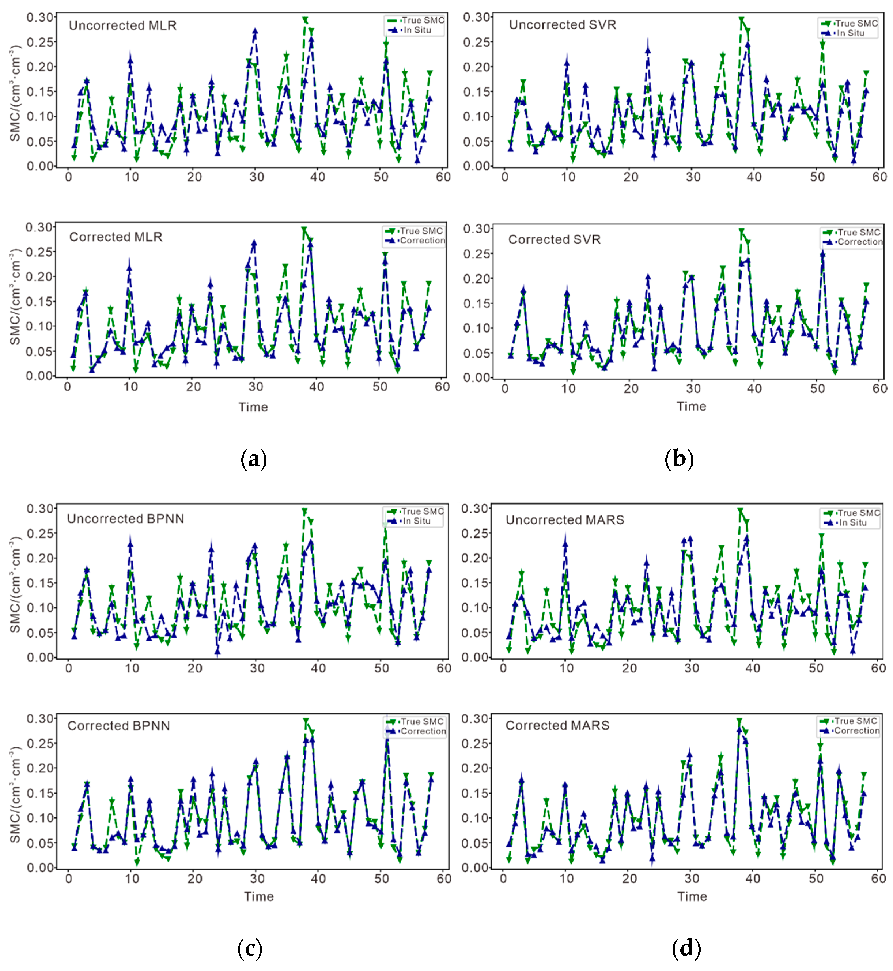
4.4. Soil Moisture Inversion Results
5. Discussion
5.1. Correction of Vegetation Error Term Analysis
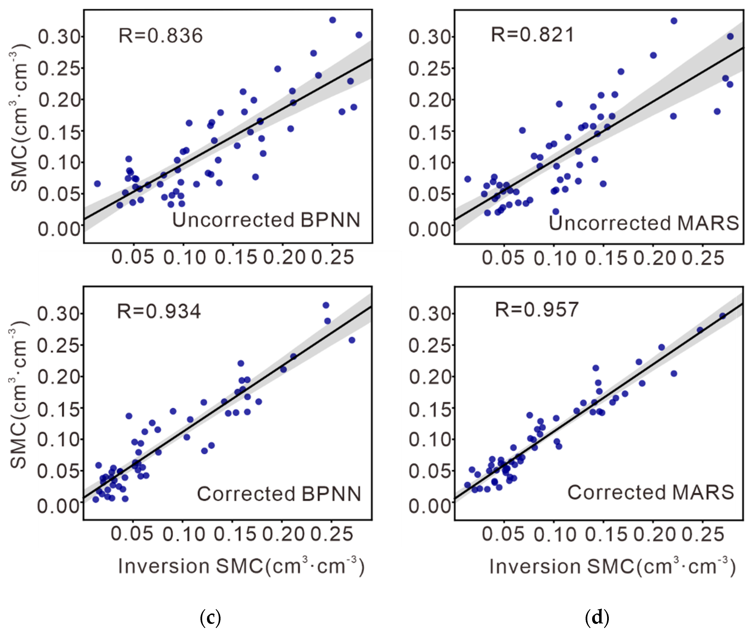
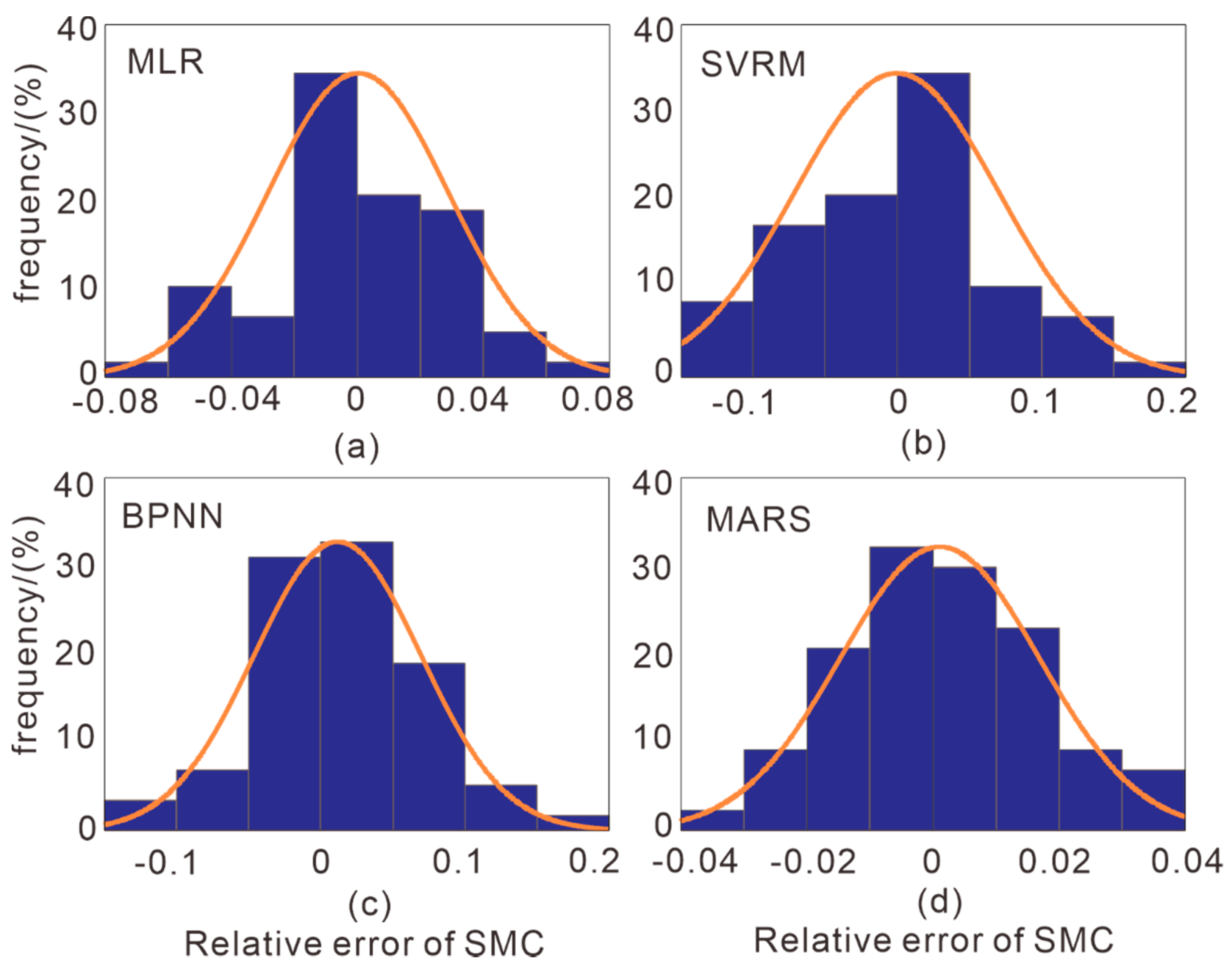
5.2. Soil Moisture Inversion Correlation Analysis
6. Conclusions
- (1)
- The NMRI that was generated based on MP1 exhibits notable periodicity and is strongly linearly correlated with the NDVI. The zeroed NDVI can adequately correct the phase shift of the reflected signal caused by vegetation.
- (2)
- The MARS algorithm fully realized the advantages of multi-satellite data integration in retrieving SMC and effectively addressed that the SMC estimated from single-satellite data cannot sufficiently reflect actual surface conditions. In addition, GCV was conducive to eliminating the satellites that significantly interfere with SMC retrievals and determining the combination of satellites with the highest SMC retrieval accuracy.
- (3)
- Compared to the SVR and BPNN models, the MARS model could obtain a combined multi-satellite expression when it was used to retrieve the SMC and had excellent generalization capability. In addition, the MARS algorithm could fully exploit its capabilities to ensure fast modeling, a relatively stable fitting process, and a relatively stable estimation error.
Author Contributions
Funding
Institutional Review Board Statement
Informed Consent Statement
Data Availability Statement
Acknowledgments
Conflicts of Interest
References
- Koster, R.D.; Dirmeyer, P.A.; Guo, Z.; Bonan, G.; Chan, E.; Cox, P.; Gordon, C.T.; Kanae, S.; Kowalczyk, E.; Lawrence, D.; et al. Regions of Strong Coupling between Soil Moisture and Precipitation. Science 2004, 305, 1138–1140. [Google Scholar] [CrossRef] [PubMed] [Green Version]
- Jackson, T.J.; Schmugge, J.; Engman, E.T. Remote sensing applications to hydrology: Soil moisture. Int. Assoc. Sci. Hydrol. 1996, 41, 517–530. [Google Scholar] [CrossRef]
- Larson, K.M.; Small, E.E. GPS ground networks for water cycle sensing. IEEE Geosci. Remote Sens. Sym. 2014, 3822–3825. [Google Scholar]
- Larson, K.M. GPS interferometric reflectometry: Applications to surface soil moisture, snow depth, and vegetation water content in the western United States. Wiley Interdiscip. Rev. Water. 2016, 3, 775–787. [Google Scholar]
- Zavorotny, V.U.; Larson, K.M.; Braun, J.J.; Small, E.E.; Gutmann, E.D.; Bilich, A.L. A Physical Model for GPS Multipath Caused by Land Reflections: Toward Bare Soil MoistureRetrievals. IEEE J. Sel. Top. Appl. Earth Observ. Remote Sens. 2010, 3, 100–110. [Google Scholar] [CrossRef]
- Larson, K.M.; Small, E.E. Normalized Microwave Reflection Index: A Vegetation Measurement Derived from GPS Networks. IEEE J. Sel. Top. Appl. Earth Observ. Remote Sens. 2014, 7, 1501–1511. [Google Scholar] [CrossRef]
- Chew, C.C.; Small, E.E.; Larson, K.M.; Zavorotny, V.U. Effects of Near-Surface Soil Moisture on GPS SNR Data: Development of a Retrieval Algorithm for Soil Moisture. IEEE Trans. Geosci. Remote Sens. 2014, 52, 537–543. [Google Scholar] [CrossRef]
- Roussel, N.; Darrozes, J.; Ha, C.; Boniface, K.; Frappart, F.; Ramillien, G. Multi-scale volumetric soil moisture detection from GNSS SNR data: Ground-based and airborne applications. MetroAeroSpace 2016, 573–578. [Google Scholar]
- Larson, K.M.; Small, E.E.; Gutmann, E.; Bilich, A.; Axelrad, P.; Braun, J. Using GPS Multipath to Measure Soil Moisture Fluctuations: Initial Results. GPS Solut. 2008, 12, 173–177. [Google Scholar] [CrossRef]
- Larson, K.M.; Small, E.E.; Gutmann, E.D.; Bilich, A.L.; Braun, J.J.; Zavorotny, V.U. Use of GPS Receivers as a Soil Moisture Network for Water Cycle Studies. Geophys. Res. Lett. 2008, 35, 24–35. [Google Scholar] [CrossRef] [Green Version]
- Larson, K.M.; Braun, J.J.; Small, E.E.; Zavorotny, V.U.; Gutmann, V.U.; Bilich, A.L. GPS Multipath and Its Relation to Near-Surface Soil Moisture Content. IEEE J. Sel. Top. Appl. Earth Observ. Remote Sens. 2010, 3, 91–99. [Google Scholar] [CrossRef]
- Chew, C.C.; Small, E.E.; Larson, K.M.; Zavorotny, V.U. Vegetation Sensing Using GPS-Interferometric Reflectometry: Theoretical Effects of Canopy Parameters on Signal-to-Noise Ratio Data. IEEE Trans. Geosci. Remote Sens. 2015, 53, 2755–2764. [Google Scholar] [CrossRef]
- Chew, C.C.; Small, E.E.; Larson, K.M. An algorithm for soil moisture estimation using GPS-interferometric reflectometry for bare and vegetated soil. GPS Solut. 2016, 20, 525–537. [Google Scholar] [CrossRef]
- Wan, W.; Larson, K.M.; Small, E.E.; Chew, C.C.; Braun, J.J. Using geodetic GPS receivers to measure vegetation water content. GPS Solut. 2015, 19, 237–248. [Google Scholar] [CrossRef]
- Small, E.E.; Larson, K.M.; Braun, J.J. Sensing vegetation growth with reflected GPS signals. Geophys. Res. Lett. 2010, 37, L12401. [Google Scholar] [CrossRef]
- Smal, E.E.; Larson, K.M.; Smith, W.K. Normalized Microwave Reflection Index: Validation of Vegetation Water Content Estimates from Montana Grasslands. IEEE J. Sel. Top. Appl. Earth Observ. Remote Sens. 2014, 7, 1512–1521. [Google Scholar] [CrossRef]
- Liang, Y.; Ren, C.; Wang, H.; Huang, Y.; Zheng, Z. Research on soil moisture inversion method based on GA-BP neural network model. Int. J. Remote Sens. 2019, 40, 2087–2103. [Google Scholar] [CrossRef]
- Small, E.E.; Larson, K.M.; Chew, C.C.; Dong, J.; Ochsner, T.E. Validation of GPS-IR Soil Moisture Retrievals: Comparison of Different Algorithms to Remove Vegetation Effects. IEEE J. Sel. Top. Appl. Earth Observ. Remote Sens. 2016, 9, 4759–4770. [Google Scholar] [CrossRef]
- Ren, C.; Liang, Y.; Lu, X.; Yan, H. Research on the soil moisture sliding estimation method using the LS-SVM based on multi-satellite fusion. Int. J. Remote Sens. 2019, 40, 2104–2119. [Google Scholar] [CrossRef]
- Lewis, P.A.W.; Stevens, J.G. Nonlinear Modelling of Time Series Using Multivariate Adaptive Regression Splines (MARS). J. Am. Stat. Assoc. 1991, 86, 864–877. [Google Scholar] [CrossRef]
- Roggenbuck, O.; Reinking, J.; Lambertus, T. Determination of Significant Wave Heights Using Damping Coefficients of Attenuated GNSS SNR Data from Static and Kinematic Observations. Remote Sens. 2019, 11, 409. [Google Scholar] [CrossRef] [Green Version]
- Bilich, A.; Larson, K.M. Mapping the GPS multipath environment using the signal-to-noise ratio (SNR). Radio Sci. 2007, 42, RS6003. [Google Scholar] [CrossRef]
- Han, M.; Zhu, Y.; Yang, D.; Hong, X.; Song, S. A Semi-Empirical SNR Model for Soil Moisture Retrieval Using GNSS SNR Data. Remote Sens. 2018, 10, 280. [Google Scholar] [CrossRef] [Green Version]
- Yuan, Q.; Li, S.; Yue, L.; Li, T.; Shen, H.; Zhang, L. Monitoring the Variation of Vegetation Water Content with Machine Learning Methods: Point–Surface Fusion of MODIS Products and GNSS-IR Observations. Remote Sens. 2019, 11, 1440. [Google Scholar] [CrossRef] [Green Version]
- Camps, A.; Alonso-Arroyo, A.; Park, H.; Onrubia, R.; Pascual, D.; Querol, J. L-Band Vegetation Optical Depth Estimation Using Transmitted GNSS Signals: Application to GNSS-Reflectometry and Positioning. Remote Sens. 2020, 12, 2352. [Google Scholar] [CrossRef]
- Evans, S.G.; Small, E.E.; Larson, K.M. Comparison of vegetation phenology in the western USA determined from reflected GPS microwave signals and NDVI. Int. J. Remote Sens. 2014, 35, 2996–3017. [Google Scholar] [CrossRef]
- Leathwick, J.R.; Elith, J.; Hastie, T. Comparative performance of generalized additive models and multivariate adaptive regression splines for statistical modelling of species. Ecol. Model. 2006, 199, 188–196. [Google Scholar] [CrossRef]
- Jakub, S.; David, I. A Generalized Estimating Equation Approach to Multivariate Adaptive Regression Splines. J. Comput. Graph. Stat. 2018, 27, 245–253. [Google Scholar]
- Hamidi, O.; Tapak, L.; Abbasi, H.; Maryanaji, Z. Application of random forest time series, support vector regression and multivariate adaptive regression splines models in prediction of snowfall (a case study of Alvand in the middle Zagros, Iran). Theor Appl Climatol. 2018, 134, 769–776. [Google Scholar] [CrossRef]
- Jin, W.; Li, Z.J.; Wei, L.S.; Zhen, H. The Improvements of BP Neural Network Learning Algorithm. In Proceedings of the IEEE 5th International Conference on Signal Processing Proceedings, Rotorua, New Zealand, 21–25 August 2000; Volume 3, pp. 1647–1649. [Google Scholar]
- Chen, P.H.; Lin, C.J.; Scholkopf, B. A tutorial on v-support vector machines. Appl. Stoch. Models. Bus. Ind. 2005, 21, 111–136. [Google Scholar] [CrossRef]


| BF No. | BF | Variable | Coefficient |
|---|---|---|---|
| BF1 | X16 | PRN16 | 0.034 |
| BF2 | Max(0, 0.065-X9) | PRN9 | 0.054 |
| BF3 | Max(0, 0.682-X9) | PRN9 | −0.507 |
| BF4 | Max(0, 0.742-X4) | PRN4 | −0.073 |
| BF5 | Max(0, 0.920-X5) | PRN5 | −0.061 |
| BF6 | Max(0, 0.995-X14) | PRN14 | −0.079 |
| BF7 | Max(0, X14-0.995) | PRN14 | −0.471 |
| BF8 | Max(0, X15-0.195) | PRN15 | −0.082 |
| BF9 | Max(0, X17-0.304) | PRN17 | 0.092 |
| BF10 | Max(0, X9-1.029) | PRN9 | 0.801 |
| BF11 | Max(0, X9-0.682) | PRN9 | −0.302 |
| Before Vegetation Correction | After Vegetation Correction | |||||||
|---|---|---|---|---|---|---|---|---|
| MLR | SVR | BPNN | MARS | MLR | SVR | BPNN | MARS | |
| R | 0.792 | 0.816 | 0.836 | 0.821 | 0.819 | 0.929 | 0.934 | 0.957 |
| RMSE | 0.126 | 0.115 | 0.076 | 0.040 | 0.096 | 0.064 | 0.051 | 0.021 |
| MAE | 0.097 | 0.086 | 0.034 | 0.032 | 0.060 | 0.045 | 0.032 | 0.017 |
Publisher’s Note: MDPI stays neutral with regard to jurisdictional claims in published maps and institutional affiliations. |
© 2021 by the authors. Licensee MDPI, Basel, Switzerland. This article is an open access article distributed under the terms and conditions of the Creative Commons Attribution (CC BY) license (https://creativecommons.org/licenses/by/4.0/).
Share and Cite
Lv, J.; Zhang, R.; Tu, J.; Liao, M.; Pang, J.; Yu, B.; Li, K.; Xiang, W.; Fu, Y.; Liu, G. A GNSS-IR Method for Retrieving Soil Moisture Content from Integrated Multi-Satellite Data That Accounts for the Impact of Vegetation Moisture Content. Remote Sens. 2021, 13, 2442. https://doi.org/10.3390/rs13132442
Lv J, Zhang R, Tu J, Liao M, Pang J, Yu B, Li K, Xiang W, Fu Y, Liu G. A GNSS-IR Method for Retrieving Soil Moisture Content from Integrated Multi-Satellite Data That Accounts for the Impact of Vegetation Moisture Content. Remote Sensing. 2021; 13(13):2442. https://doi.org/10.3390/rs13132442
Chicago/Turabian StyleLv, Jichao, Rui Zhang, Jinsheng Tu, Mingjie Liao, Jiatai Pang, Bin Yu, Kui Li, Wei Xiang, Yin Fu, and Guoxiang Liu. 2021. "A GNSS-IR Method for Retrieving Soil Moisture Content from Integrated Multi-Satellite Data That Accounts for the Impact of Vegetation Moisture Content" Remote Sensing 13, no. 13: 2442. https://doi.org/10.3390/rs13132442
APA StyleLv, J., Zhang, R., Tu, J., Liao, M., Pang, J., Yu, B., Li, K., Xiang, W., Fu, Y., & Liu, G. (2021). A GNSS-IR Method for Retrieving Soil Moisture Content from Integrated Multi-Satellite Data That Accounts for the Impact of Vegetation Moisture Content. Remote Sensing, 13(13), 2442. https://doi.org/10.3390/rs13132442