Early Identification of Root Rot Disease by Using Hyperspectral Reflectance: The Case of Pathosystem Grapevine/Armillaria

Abstract

Armillaria genus represents one of the most common causes of chronic root rot disease in woody plants. Prompt recognition of diseased plants is crucial to control the pathogen. However, the current disease detection methods are limited at a field scale. Therefore, an alternative approach is needed. In this study, we investigated the potential of hyperspectral techniques to identify fungi-infected vs. healthy plants of Vitis vinifera. We used the hyperspectral imaging sensor Specim-IQ to acquire leaves’ reflectance data of the Teroldego Rotaliano grapevine cultivar. We analyzed three different groups of plants: healthy, asymptomatic, and diseased. Highly significant differences were found in the near-infrared (NIR) spectral region with a decreasing pattern from healthy to diseased plants attributable to the leaf mesophyll changes. Asymptomatic plants emerged from the other groups due to a lower reflectance in the red edge spectrum (around 705 nm), ascribable to an accumulation of secondary metabolites involved in plant defense strategies. Further significant differences were observed in the wavelengths close to 550 nm in diseased vs. asymptomatic plants. We evaluated several machine learning paradigms to differentiate the plant groups. The Naïve Bayes (NB) algorithm, combined with the most discriminant variables among vegetation indices and spectral narrow bands, provided the best results with an overall accuracy of 90% and 75% in healthy vs. diseased and healthy vs. asymptomatic plants, respectively. To our knowledge, this study represents the first report on the possibility of using hyperspectral data for root rot disease diagnosis in woody plants. Although further validation studies are required, it appears that the spectral reflectance technique, possibly implemented on unmanned aerial vehicles (UAVs), could be a promising tool for a cost-effective, non-invasive method of Armillaria disease diagnosis and mapping in-field, contributing to a significant step forward in precision viticulture.

1. Introduction

The Armillaria (Fr.: Fr.) Staude is a globally distributed and widely studied genus of pathogenic fungus belonging to the Basidiomycota class, Agaricales order, and Tricholomataceae family [1,2]. It spreads under the soil through root contact or complex structures named rhizomorphs, which can grow relatively fast for a hundred meters and penetrate the root bark of the hosts [3,4]. Armillaria spp. are opportunistic parasites; however, some species, such as A. mellea (Vahl) P. Kumm., are considered the primary parasites of stressed trees [5] and are going to increase their damage under climate change conditions [6]. Moreover, the modern context of agricultural intensification may offer an opportunity for Armillaria to adapt to single monocultures with a resulting disease grimness amplification [5]. Armillaria spp. can parasitize a wide range of plant species in forests, both conifers and broadleaves [7], and in garden trees and shrubs [8], and it can cause extensive losses in fruit orchards, such as apples and berries [9], pears [10], peaches [11,12], and kiwifruits [13], as well as grapevines [14,15,16,17].

1.1. Root Symptoms

The host infection normally has a chronic course, resulting in a rot collar and roots that lead to its death after several years [5]. Roots appear dark, are easily removable from the ground, and have a fibrous consistency [18,19]. Furthermore, it is possible to perceive a strong scent of fresh mushrooms by smelling the roots, especially in humid conditions [20]. By scratching the collar and main roots’ bark with a small knife, it is possible to notice a white mycelium that ends in the typical fan shape (Figure 1). Dark brown rhizomorphs can be found in roots and soil. The presence of fruiting bodies is sporadic in the vineyard and could occur exclusively in autumn and after several years of infection [20].

1.2. Foliar Symptoms

While the observation of plant collars could be sufficient to obtain an accurate diagnosis [18], on the other hand, the disease is not easily ascribed from foliar symptoms themselves due to their unspecificity. Additionally, foliar symptoms become visible when the diseased have reached an advanced stage and the host has been compromised [14]. According to Baumgartner et al. [14], foliar symptoms do not appear until one-half to three-quarters of the main host root is colonized by Armillaria mellea. Aboveground Armillaria symptoms in grapevines include lower plant vigor and low fruit production with a generally suffering appearance, a higher number of lateral shoots, dwarf, and wilting leaves, and stunted and not lignified shoots [14,18,20].

1.3. Disease Diagnosis

Since there are no effective plant protection products on the market to control the pathogen [7], disease assessment is crucial for pest management. In fact, an accurate diagnosis in the field will improve the efficiency of prophylactic methods [5,21], such as the prompt elimination of infected plants, root residual removal, crop rotations, and the use of less susceptible rootstocks [16]. Traditionally, the disease damage assessment was estimated using a visual approach, relying upon direct observation in the vineyard. However, this method is time consuming, labor intensive, and costly for disease monitoring in large-scale farming. Consequently, there is a need to develop new approaches that can enhance or supplement traditional techniques. Additionally, early disease detection would increase the effectiveness of preventive measures typically used to face the pathogen. This study aims to investigate the potential of an alternative and non-destructive method to detect root rot disease in grapevines early.

1.4. The Potential of Hyperspectral Sensors

Hyperspectral technology may represent a valuable alternative to traditional disease assessment and has proven to be a promising tool for disease diagnosis [22]. The use of spectral sensors for crop disease assessment started many decades ago. In the early 1980s, Toler et al. [23] used aerial color infrared photography to evaluate root rot disease of cotton and wheat stem rust. Reflectance data turned out to be capable of detecting pathogen-induced biophysical-specific changes in the plant leaf and canopy [24]. Since then, however, remote sensing technologies have significantly progressed, and, in 2020, the possibility to automatically classify cotton root rot disease based on unmanned aerial vehicles (UAVs) was reported for the first time [25]. Modern hyperspectral imaging sensors with super spatial, spectral, and radiometric resolutions offer enhanced capabilities to detect and map disease symptoms on a large scale. These sensors capture reflectance characteristics of the target materials and the reflected light recorded with a high spectral and spatial resolution [26]. The recent advances in hyperspectral imaging sensors are expected to improve disease detection, because they allow a pixel-wise attribution of disease-specific symptoms and healthy tissue [27]. In this context, different spectral methods used to evaluate the vegetation status both quantitatively and qualitatively and vegetation indices (VIs) are among the most common [26].

Several recent studies, using different sensors, have confirmed the potential of hyperspectral data to detect plant pathologies in a reliable manner in various pathosystems associated with grapevines, such as leafroll-associated virus-3 [22,28,29], grapevine trunk disease [30,31,32], Flavescence dorèe [33,34,35], and powdery mildew [36]. However, to date, there are no available data concerning grapevine root rot disease identification through hyperspectral images, thus making this work the pioneer.

The hyperspectral imaging sensor Specim IQ that we used in our study has a wide variety of applications in remote sensing and precision agriculture. This sensor is used to study, in a non-invasive manner, the physiology, architecture, and biochemistry of crop plants or natural vegetation in different environmental conditions and on different scales. For instance, it was implemented for stress detection in plant phenotyping processes and in plant pigment composition studies. The camera can be considered a novel valuable tool for hyperspectral imaging use in the context of plant research and phenotyping strategies [26]. In a recent publication, the sensor was used to detect a common root rot pathogen (Bipolaris sorokiniana) affecting the seedlings of wheat [37]. Analogously, Barreto et al. [38] used this sensor for measuring the root rot disease incidence in celery leaves caused by Rhizoctonia solani.

In this study, we analyzed the leaf level reflectance of grapevine cv. Teroldego Rotaliano from diseased, healthy, and asymptomatic plants to understand whether there are characteristic spectral changes, across the visible and near-infrared (NIR) domains, associated with the infection. We assumed that leaf reflectance provides relevant information to identify Armillaria infections in grapevines even though foliar symptoms are not yet visible.

2. Materials and Methods

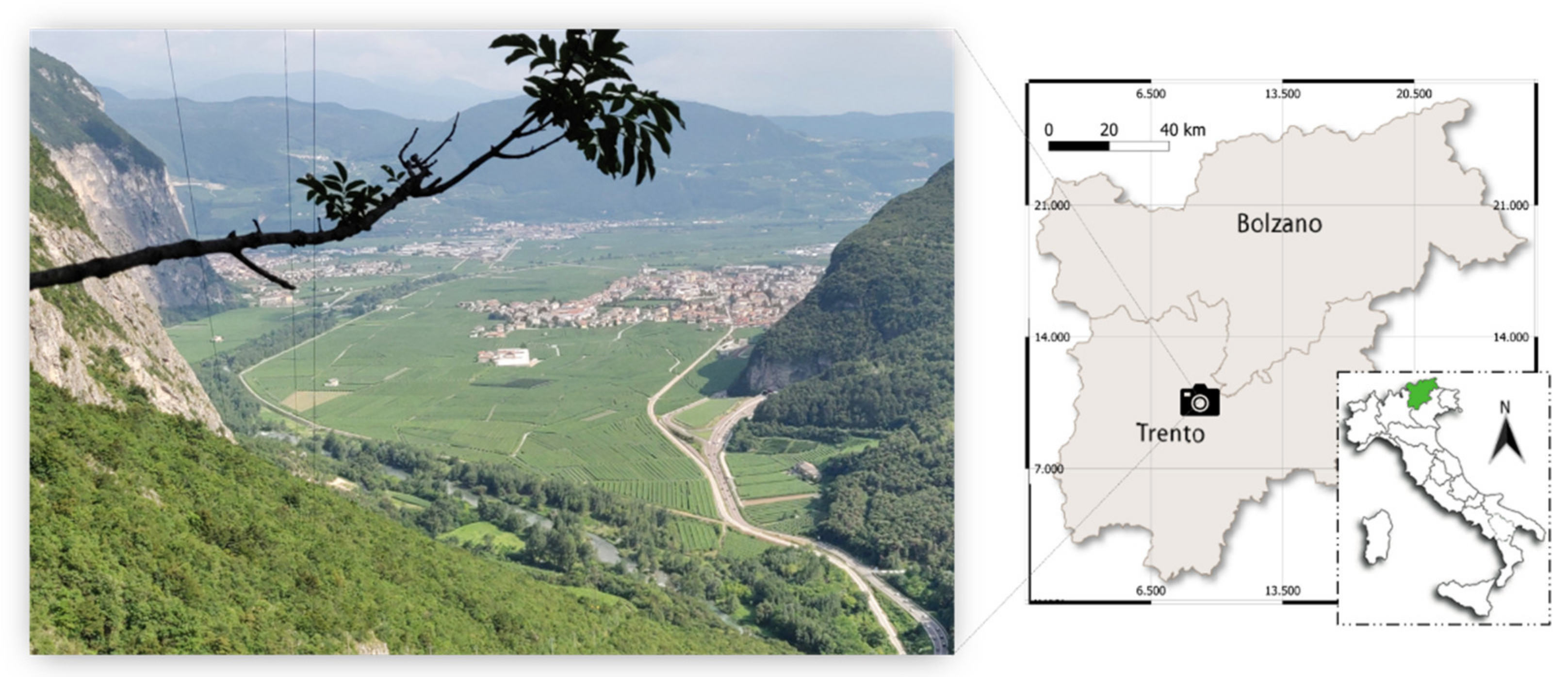
2.1. Study Site

The vineyard object of study is located in the Piana Rotaliana on the northeast side of Italy (Figure 2). The Piana Rotaliana is a winegrowing region where Armillaria mellea has been a grave problem for several years [15]. The surface is predominantly cultivated with the native red grape variety named Teroldego Rotaliano (about 2000 ha). The soil is characterized by a good water drainage capacity [20], and it is classified as post-glacial alpine [39] formed in the Pleistocene age by deposits from glaciers, landslides, rock glaciers, and alluvial debris, with a sandy and gravelly texture.

The selected vineyard is located on the northeast of Piana Rotaliana (46°13′36″N, 11°04′39″E) at 250 m a.s.l., and it was planted in 2005 with the native grape variety Teroldego Rotaliano. The vines were grafted into Teleki 5C rootstock, while the training system was the double pergola. The vine spacing was 5 m × 0.8 m, the rows were oriented ca. east–west. We found the typical fan mycelium attributable to Armillaria spp. in several plants within the vineyard and, more rarely, rhizomorphs in their collars. The vineyard was uprooted at the end of the season in 2019, and this allowed us to collect and thoroughly examine the vine roots.

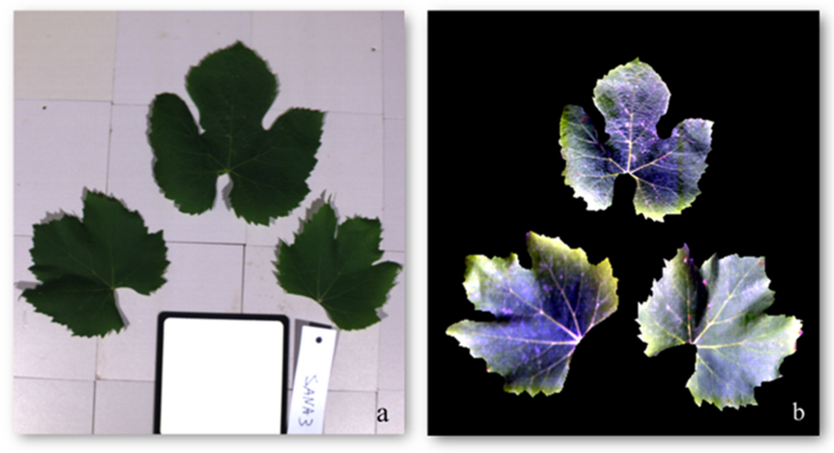
2.2. Foliar Sampling

We collected three fresh leaves for each plant in the first week of September 2019, (between 9 p.m. and 11 p.m.). Once detached, the leaves were immediately placed in a refrigerated thermic box at 6 °C, and then transported to the Spectra lab and stored in darkness at 6 °C before spectral measurements were taken [32]. They were analyzed within two hours after field collection. We used a controlled foliar selection process in order to minimize the variability among the plants and compare equal leaves. We collected the leaves from the first branch of lateral shoots, generally located between the third and the fourth vineyard trellis wires. We exclusively harvested mature leaves with a well-exposed upper sheet to sunlight. Moreover, we made sure they were physically intact, apparently healthy on both faces, and they all had approximately homogeneous sizes. Furthermore, plants suspected to be infected by other pathogens were previously excluded.

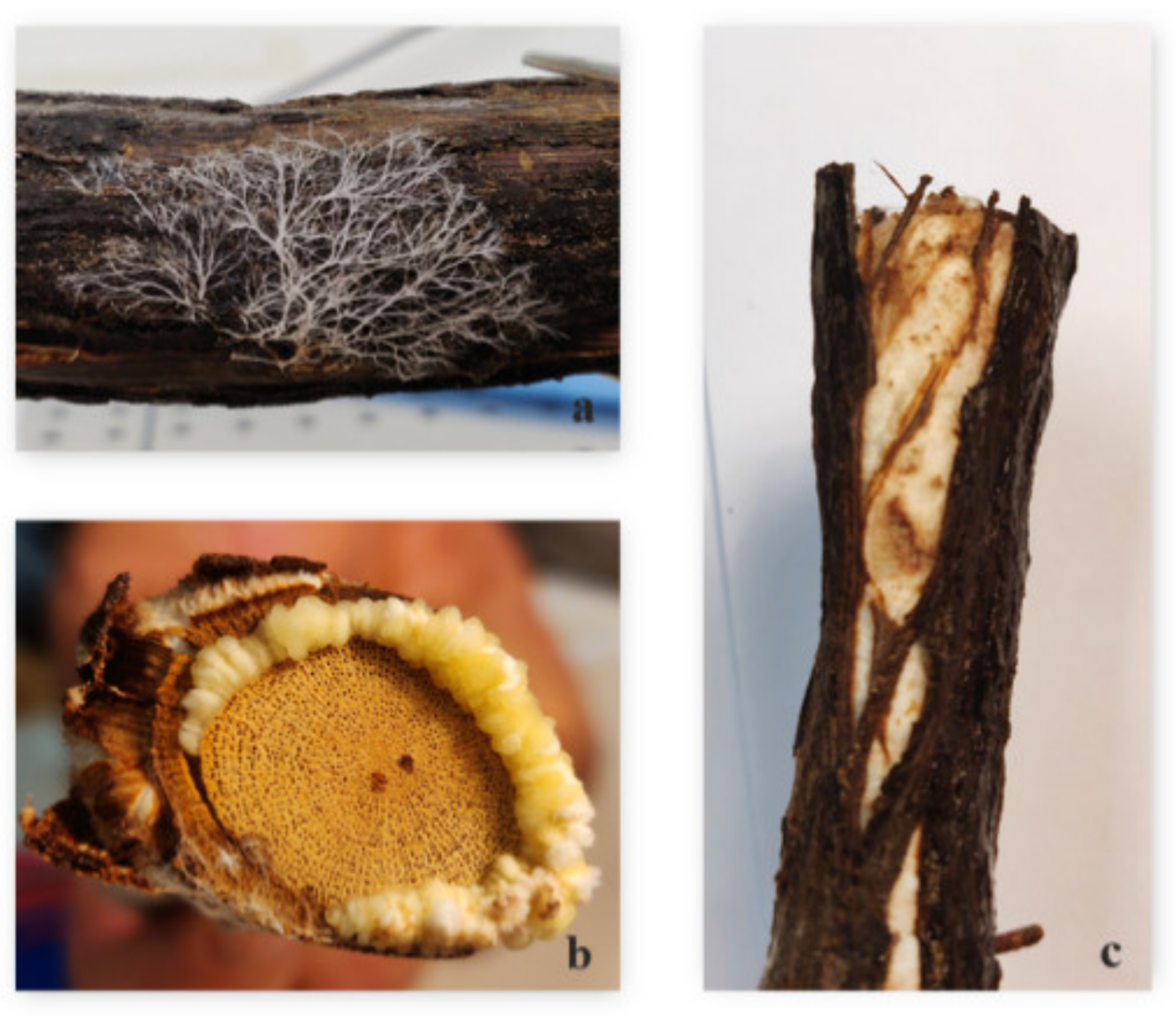
2.3. Root Sampling and Inspection

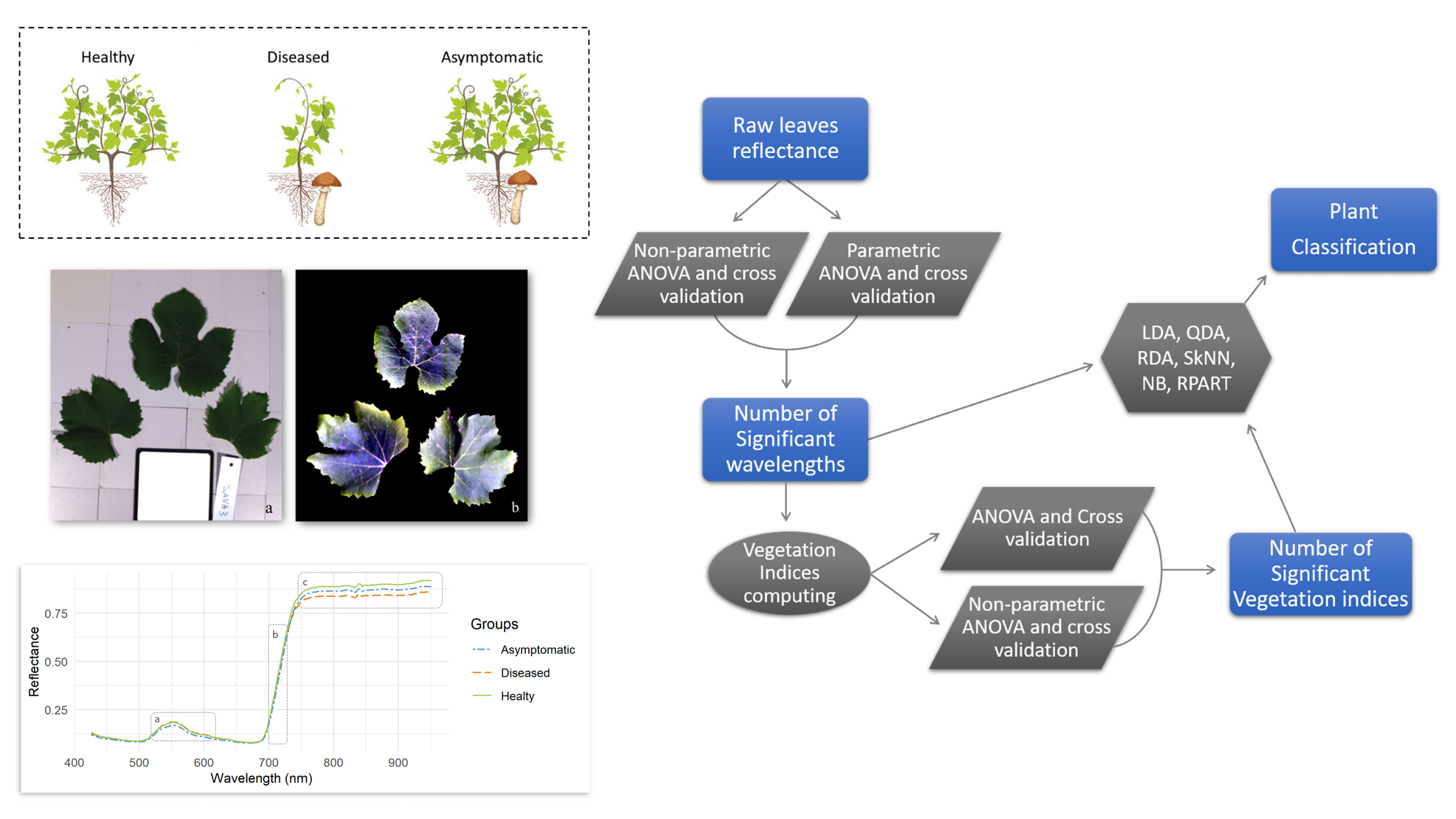
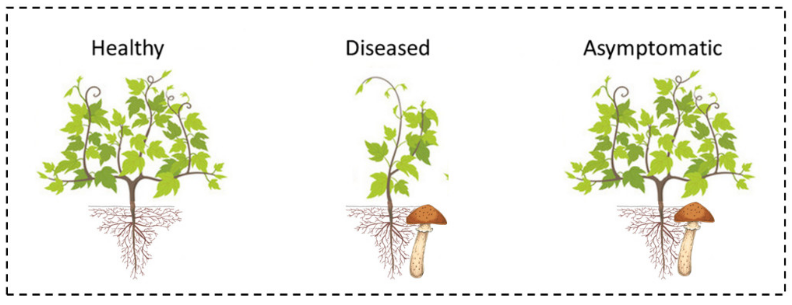
The grapevines were uprooted in the first week of October 2019, using a mechanical excavator. Plant roots were visually assessed, and three portions about 7–8 cm long with a diameter from 1.5 cm to 3.0 cm were taken as a sample for each plant. The portions were chosen from rot or suspected areas. Roots without any evidence of root rot were also collected. We thoroughly washed the samples using fresh and clean water to remove soil debris and disinfected them with the following procedure. They were soaked in a backer with a solution of 30% of a commercial preparation of sodium hypochlorite (NaOCl concentration 5%), 70% of sterile water, and 0.01% of Tween-20 for 5 min, while the liquid was kept with agitation by a magnetic anchor at room temperature. After disinfection, the roots were washed twice for two minutes with sterile water in a sterile backer and then rinsed. At this point, they were incubated in humid chambers made of transparent sterile nylon bags inflated by air and wet paper inside. We kept the humid chambers in closed boxes placed in a dark room for about a month until the final visual disease assessment based on mycelium growth. For the species identification, we relied on Pertot et al. [40].

2.4. Plant Groups

For the plant grouping, we matched the foliar and root symptoms of each vine as in Figure 3. Healthy plants were those without symptoms either in canopy or roots, diseased plants were those with symptoms in leaves and the presence of Armillaria mellea in roots, and asymptomatic plants were those without any foliar symptoms but infected by the pathogen and in closest proximity to the diseased ones. In total, we selected 35 grapevines for the sample, from which 7 were healthy, 12 diseased, and 16 asymptomatic.

2.5. Hyperspectral Data Acquisition

We used the hyperspectral camera Specim IQ (Specim, Spectral Imaging Ltd., Oulu, Finland) to measure leaf reflectance. Specim IQ is a portable sensor capable of acquiring the reflected electromagnetic radiation from an object in 204 narrow bands with a spectral range from 397 nm to 1003 nm, a spectral resolution of 7 nm, and a spectral sampling of 3.5 nm. It performs the measurements by lines scanning 512 pixels and records the image in a square with a resolution of 512 × 512 px.

The sensor was placed on its tripod ground base at 74 cm from the ground, and nadir images were collected. The measurements were conducted in a dark room, where light was provided by two Helder Systemlicht C12 halogen lamps (Helder Systemlicht GmbH, Runkel/Lahn, Germany) placed toward the leaves at 120 cm height. The camera shutter speed was set at 13 milliseconds per pixel, corresponding to 36 s per photo. We performed spectral data acquisition including three leaves in each image. The leaves were placed on the ground with the upper surface oriented upwards, as shown in Figure 4, and arranged with the Spectralon panel nearby used for white calibration. The use of the white reference target ensures the calibration of the radiance images though the SPECIM camera software, which provides calibrated reflectance imagery as an output. We cut petioles to properly expand the leaves on the ground before spectral analyses.

We analyzed the images using ENVI software (L3Harris Geospatial Solutions Inc., Broomfield, CO, USA). First, we extracted the leaves as the region of interest (ROI) and excluded background pixels. Then, we calculated the mean reflectance of the leaves, by averaging all pixel values included in the ROI. Noisy bands at the tails from 397 nm to 423 nm and bands from 954 nm to 1003 nm were eliminated, minimizing the background noise [38].

In this study, we calculated a set of 18 VIs potentially capable of discriminating against infected and uninfected vines.

Table 1. Vegetation indices used for measuring reflectance changes between leaves from asymptomatic, diseased, and healthy plants of armillaria-diseased grapevines.

Number	Vegetation Index	Abbreviation	Equation	Related to	Reference
1	Anthocyanin Reflectance Index	ARI	${\left(R_{551}\right)}^{-1}-{\left(R_{705}\right)}^{-1}$	anthocyanins	[43]
2	Modified Anthocyanin Reflectance Index	mARI	$\left({\left(R_{551}\right)}^{-1}-{\left(R_{710}\right)}^{-1}\right)\times R_{951}$	anthocyanins	[44]
3	Carotenoid Reflectance Index Red Edge	mCRIRE	$\left({\left(R_{520}\right)}^{-1}-{\left(R_{700}\right)}^{-1}\right)\times R_{951}$	carotenoid	[44]
4	Normalized Difference Chlorophyll	NDchl	$\left(R_{925}-R_{710}\right)/\left(R_{925}+R_{710}\right)$	chlorophyll	[45]
5	Red Edge Inflection Point 3	REIP3	$\left(\left(\left(R_{665}+R_{783}\right)/2\right)-R_{705}\right)/\left(R_{740}+R_{705}\right)$	chlorophyll	[46]
6	Leaf Chlorophyll Index	LCI	$\left(R_{850}-R_{710}\right)/\left(R_{850}+R_{680}\right)$	chlorophyll	[47]
7	Vogelmann Indices 2	Vog2	$\left(R_{734}-R_{747}\right)/\left(R_{715}+R_{726}\right)$	chlorophyll	[24]
8	Zarco-Tejada and Miller	SR750/710	$R_{750}/R_{710}$	chlorophyll	[48]
9	Chlorophyll Red Edge	Chlred-edge	${\left(R_{771}/R_{711}\right)}^{-1}$	chlorophyll	[44]
10	Difference Vegetation Index	DVI	$R_{951}/R_{640}$	vegetation	[49]
11	Normalized Difference Vegetation Index	NDVI	$\left(R_{932}-R_{604}\right)/\left(R_{604}+R_{932}\right)$	vegetation	[49]
12	Misra Green Vegetation Index	MGVI	$-0.386\left(R_{500}\right)-0.530\left(R_{600}\right)+0.535\left(R_{800}\right)+0.532\left(R_{951}\right)$	vegetation	[49]
13	Green Normalized Difference Vegetation Index	GNDVI	$\left(R_{570}-R_{800}\right)/\left(R_{570}+R_{800}\right)$	vegetation	[50]
14	Ashburn Vegetation Index	AVI	$2.0\times \left(R_{951}\right)-\left(R_{600}\right)$	vegetation	[49]
15	Green Difference Vegetation Index	GDVI	$R_{566}-R_{902}$	vegetation	[51]
16	Optimized Soil-Adjusted Vegetation Index	OSAVI	$\left(1+0.16\right)/\left(\left(R_{902}-R_{672}\right)/\left(R_{902}+R_{672}+0.16\right)\right)$	vegetation	[48]
17	Simple Ratio Carter4	Ctr4	$R_{710}/R_{760}$	stress	[52]
18	Water Band Index	WBI	$R_{970}/R_{902}$	water content	[42]

includes the equations and the references for every selected VI. Some VIs are used in the literature to detect leaf chlorophyll content (NDchl, REIP3, LCI, Chlred-edge, Vog2, SR750/710), while others are correlated with anthocyanin content (mARI, ARI) and carotenoid content (mCRIRE). Further computed VIs are normally used to retrieve other key vegetation parameters, e.g., plant status or biomass (NDVI, GNDVI, AVI, MGVI, DVI, GDVI, OSAVI). Lastly, the index Ctr4 linked to plant-related stresses [41] and the water band index (WBI) linked to the water content [42] were computed.

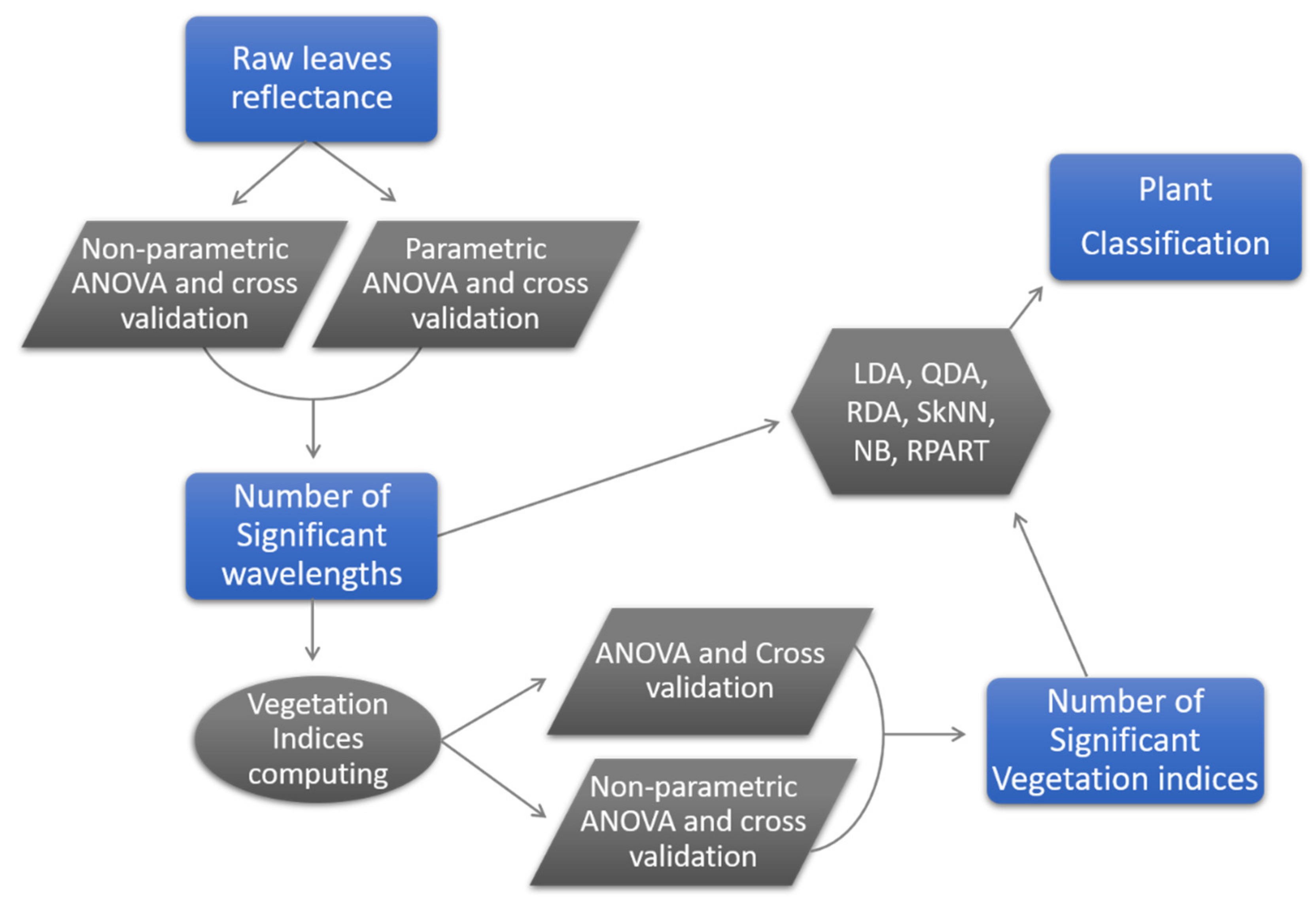
2.6. Statistical Analyses

In a preliminary analysis, we calculated the standard deviation within each group of plants with the following Equation (1):

$$\sigma =\sqrt{\frac{\sum {\left(X-\overline{X}\right)}^2}{n}}$$

(1)

where X represents the single plant reflectance, $\overline{X}$ represents the group-averaged reflectance, and n represents the number of plants within the group.

Afterward, we performed an inferential statistical analysis in three different steps as shown in Figure 5. In step 1, we identified the most relevant wavelengths to discriminate diseased, healthy, and asymptomatic groups. For this purpose, we used the same statistical approach used in Manevski et al. [53] to discriminate different types of vegetation. In this approach, we performed both parametric and non-parametric ANOVA (Kruskal–Wallis) tests for every single wavelength. Afterward, we performed the respective parametric and non-parametric cross-validations using Tukey HSD and the Wilcox test.

In step 2, we computed and selected the most relevant VIs to separate the groups of plants. In order to do so, we relied on Naidu et al. [28], and Avola et al. [54]; however, since not all of the data were normally distributed, we performed a non-parametric ANOVA test in addition to the parametric ANOVA suggested by the authors. Before performing the statistical tests, we verified assumptions of the ANOVA using Shapiro and Bartlett tests [55,56]. Afterward, we performed the respective parametric and non-parametric cross-validations using Tukey HSD and the Wilcox test.

In step 3, we tested and validated several machine learning classification paradigms based on a combination of the first five most discriminant variables among spectral bands and VIs. The variables’ discrimination power was evaluated according to the ANOVA test and cross-validation results (see

Table A1. Non-parametric ANOVA and its relative cross-validation results for the VIs.

No.	Index	p-Value	Diseased vs. Asymptomatic	Healthy vs. Asymptomatic	Healthy vs. Diseased
			Cross-Validation P-adj
1	GDVI	0.000004	0.00005	0.52294	0.00002
2	MGVI	0.00004	0.00130	0.27417	0.00009
3	OSAVI	0.00009	0.00016	1	0.00259
4	NDchl	0.00011	0.00009	0.05128	0.35577
5	mARI	0.00012	0.00004	0.87102	0.05249
6	Ctr4	0.00016	0.00019	0.02559	0.60489
7	Chlred-edge	0.00016	0.00018	0.03003	0.58745
8	REIP3	0.00019	0.00045	0.00916	0.95927
9	SR750/710	0.00020	0.00026	0.02886	0.58745
10	GNDVI	0.00021	0.00014	0.19992	0.15410
11	NDVI	0.00021	0.00008	0.49839	0.13671
12	LCI	0.00023	0.00023	0.05320	0.43261
13	AVI	0.00025	0.03044	0.09668	0.00014
14	DVI	0.00039	0.00014	0.88900	0.11608
15	Vog2	0.00122	0.00155	0.04942	1.00000
16	mCRIRE	0.00219	0.05001	0.25925	0.00276
17	ARI	0.00908	0.00451	0.98258	0.62269
18	WBI	0.15533	0.22688	0.70442	1

and

Table A2. Parametric ANOVA and its relative cross-validation results for the VIs.

No.	Index	p-Value	F-Value	Diseased vs. Asymptomatic	Healthy vs. Asymptomatic	Healthy vs. Diseased
				Cross-Validation P-adj
1	GDVI	6.6 × 10−7	16.42	1.4 × 10−5	5.0 × 10−1	8.7 × 10−6
2	NDchl	1.2 × 10−5	12.69	6.7 × 10−6	6.3 × 10−2	1.6 × 10−1
3	MGVI	1.3 × 10−5	12.63	4.3 × 10−4	3.0 × 10−1	3.9 × 10−5
4	OSAVI	1.4 × 10−5	12.50	9.6 × 10−5	7.4 × 10−1	1.7 × 10−4
5	GNDVI	1.5 × 10−5	12.42	7.6 × 10−6	1.7 × 10−1	6.6 × 10−2
6	NDVI	1.7 × 10−5	12.24	9.00 × 10−6	2.50 × 10−1	4.26 × 10−2
7	LCI	1.8 × 10−5	12.17	1.0 × 10−5	7.2 × 10−2	1.7 × 10−1
8	Ctr4	2.0 × 10−5	12.07	1.3 × 10−5	3.8 × 10−2	2.8 × 10−1
9	REIP3	2.2 × 10−5	11.94	1.5 × 10−5	3.5 × 10−2	3.1 × 10−1
10	Chlred.edge	2.6 × 10−5	11.71	2.0 × 10−5	3.1 × 10−2	3.6 × 10−1
11	mARI	2.8 × 10−5	11.62	1.7 × 10−5	4.3 × 10−1	2.4 × 10−2
12	SR750.710	3.7 × 10−5	11.30	2.8 × 10−5	3.2 × 10−2	4.0 × 10−1
13	AVI	7.3 × 10−5	10.47	7.6 × 10−3	1.0 × 10−1	7.2 × 10−5
14	DVI	9.1 × 10−5	10.21	5.4 × 10−5	4.4 × 10−1	4.3 × 10−2
15	Vog2	2.7 × 10−4	8.90	2.6 × 10−4	3.9 × 10−2	6.3 × 10−1
16	mCRIRE	2.5 × 10−3	6.35	6.5 × 10−2	1.9 × 10−1	2.1 × 10−3
17	ARI	5.5 × 10−3	5.47	3.7 × 10−3	4.7 × 10−1	2.8 × 10−1
18	WBI	2.8 × 10−1	1.28	3.0 × 10−1	5.0 × 10−1	9.9 × 10−1

for p-values of VIs and Table S1 for p-values of wavelengths). We verified data assumptions using the Shapiro test and Box’s M test, and statistical transformations were made (Table S2). In this work, we used six multi-class classification methods, both linear and non-linear, in order to identify the most powerful method for detecting Armillaria disease. The classifiers used were the following: linear discriminant analysis (LDA), quadratic discriminant analysis (QDA), regularized discriminant analysis (RDA), simple k-nearest neighbor (SkNN), Naïve Bayes (NB), and recursive partitioning regression tree (RPART). The LDA classifier develops a linear boundary by fitting a multivariate normal density with pooled covariance estimates for each class [54,57,58,59,60,61,62], whereas the QDA is a non-linear model that constructs a non-linear boundary by fitting multivariate normal densities with covariance estimates separated by groups [58,61]. The LDA is a simple model that works better while classifying small sample sizes and requires a shorter computation time, whereas the QDA is better suited for a complex dataset. Afterward, we operated the regularized discriminant analysis (RDA) with the intent to optimize the model. The RDA function builds a classification rule using regularized group covariance matrices that are supposed to be more robust against multicollinearity in the data [63,64]. The SkNN is a broadly used machine learning algorithm that works well on simple recognition problems in supervised learning [59]. It is one of the most straightforward classification algorithms, and it can be used for classification and regression problems, providing highly competitive results. In SkNN, each neighbor is assigned with a contribution weight so that the nearer neighbors contribute more than the distant ones to the average [65,66]. The NB classifier is a probabilistic statistical classification method, which is based on the application of the Bayes theorem (Bayesian statistics) [58,67]. The RPART is a potent and simple algorithm similar to the regression trees used by Breiman et al. (1984) [68], which differs mainly from its handling of surrogate variables. In this study, the dataset was randomly split into two parts, where 65% was used as a training set while the remaining 35% as a validation set.

2.7. Accuracy Assessment

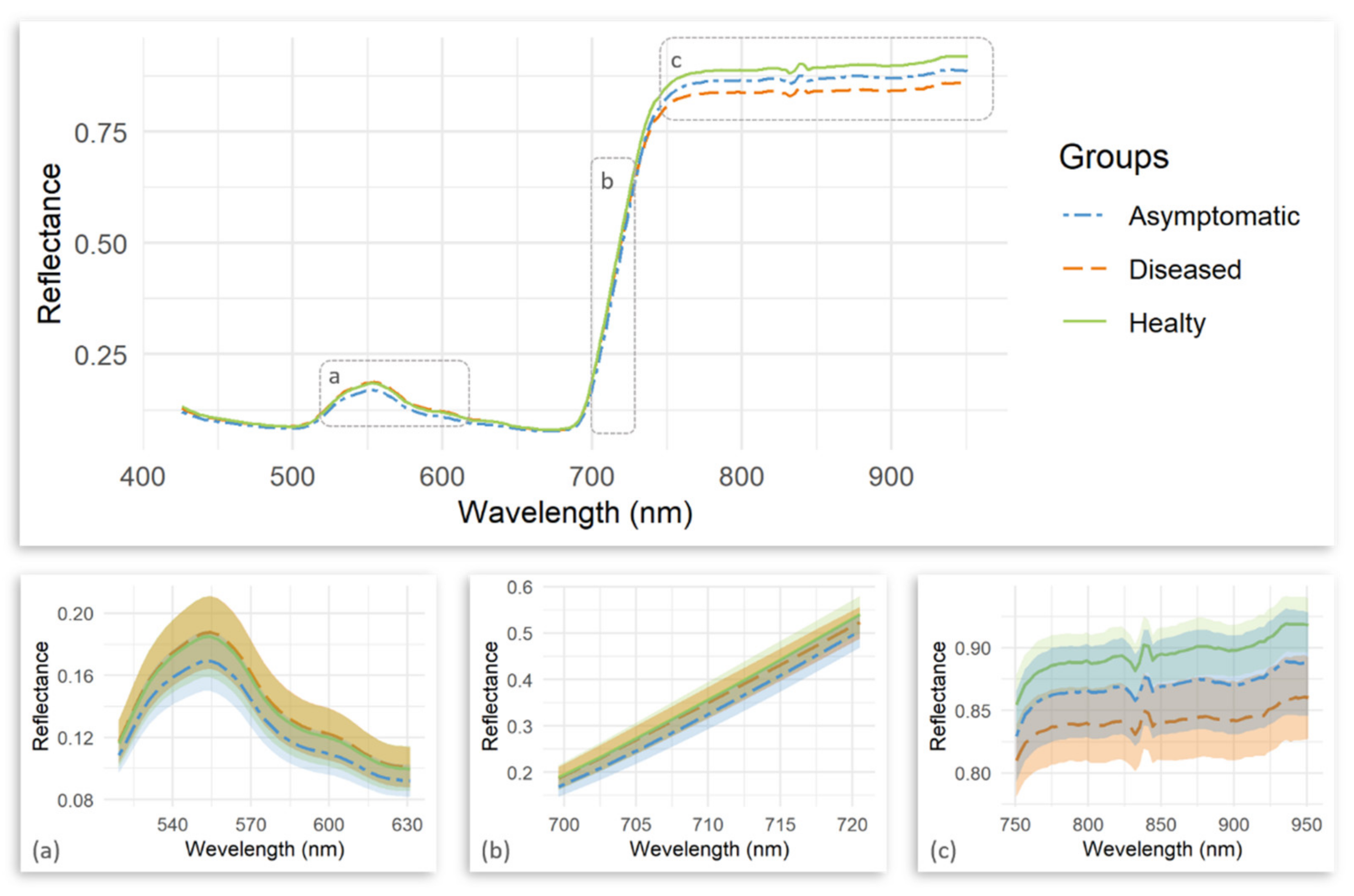
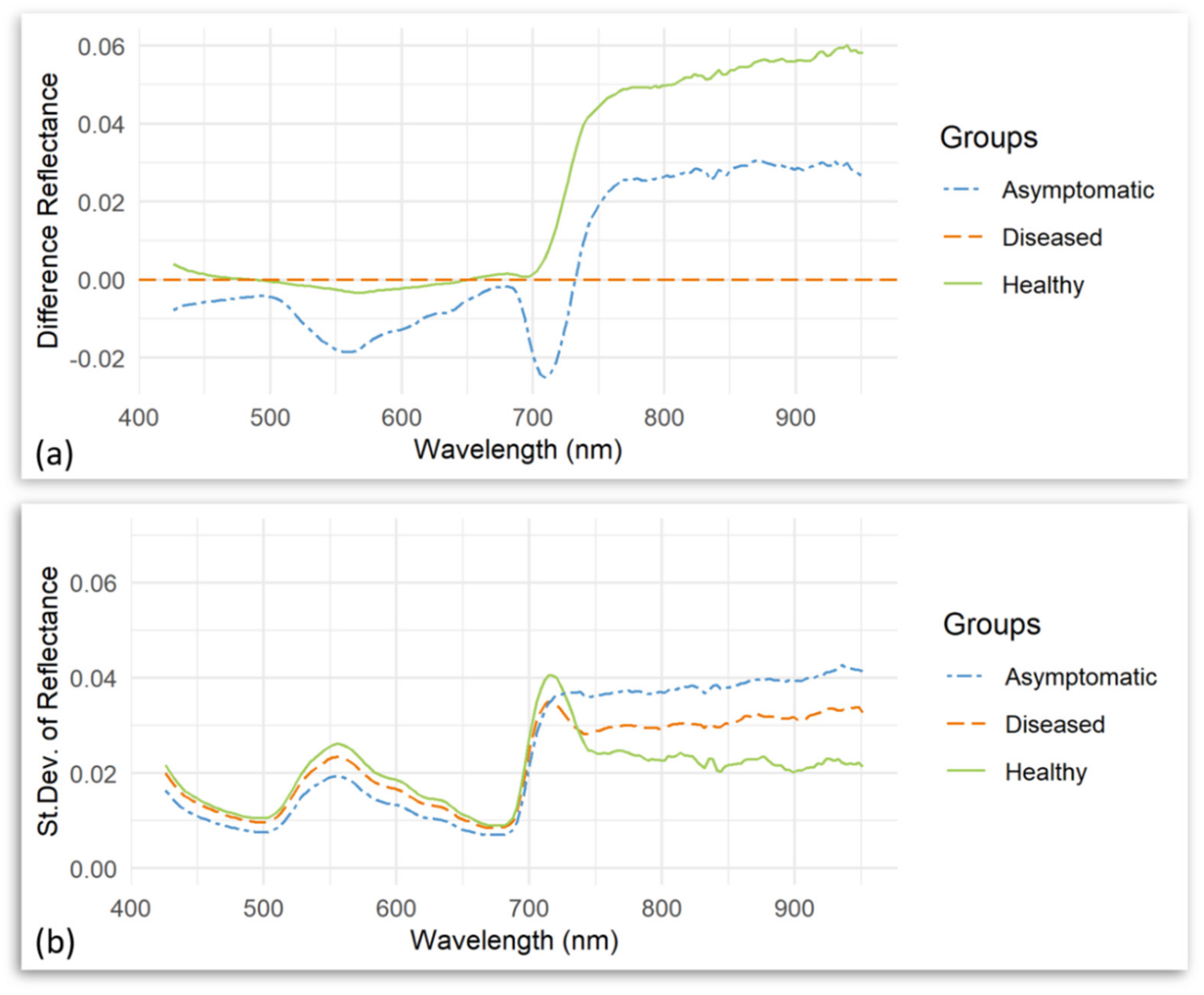
Accuracy assessment is an indispensable procedure to evaluate classification performance [25]. To assess the accuracy of classifications, the confusion matrix was generated including the overall accuracy (OA) in Equation (2), error of omission (EO) in Equation (3), error of commission (EC) in Equation (4), and the kappa coefficient. Errors of omission refer to plants that belong to a class but are not classified into that class. For example, a high omission error of the diseased group means that a large number of Armillaria-infested plants are classified healthy. This error is termed producer’s accuracy. Errors of commission refer to plants that belong to one class but are classified into another class. For example, a high commission error of the diseased group means that many healthy plants are misclassified as Armillaria-infected plants. For an accurate classification, both omission and commission errors should be at a low level. The accuracy metrics were calculated using the following formulas:

$$\mathrm{Overall} \mathrm{Accuracy} \left(\%\right)=\left[\frac{\left(\mathrm{TP}+\mathrm{TN}\right)}{\left(\mathrm{TP}+\mathrm{TN}+\mathrm{FP}+\mathrm{FN}\right)}\right]\times 100$$

(2)

$$\mathrm{Omission} \mathrm{Error} \left(\%\right)=\left[\frac{\mathrm{FN}}{\mathrm{FN}+\mathrm{TP}}\right]\times 100$$

(3)

$$\mathrm{Commision} \mathrm{Error} \left(\%\right)=\left[\frac{\mathrm{FP}}{\mathrm{FP}+\mathrm{TP}}\right]\times 100$$

(4)

where TP and TN are true positive (diseased correctly detected) and true negative (healthy plants correctly detected), respectively. FP and FN are mean false positive (healthy plants detected as diseased) and false negative (diseased plants detected as healthy), respectively. All the statistical analyses were carried out using R studio.

3. Results

After the incubation period, we found the Armillaria spp. mycelium in roots of both diseased and asymptomatic grapevines. Figure 6a shows the white Armillaria mycelium with its typical fan shape growing outside the root bark. Figure 6b,c illustrate the mycelium growing under the root bark that, in turn, is cracked by the radial expansion of the pathogen.

Once we grouped the plants into healthy, diseased, and asymptomatic groups according to their root and foliar symptoms, we measured their leaf reflectance and then calculated the spectral averages for each group. The resulting mean hyperspectral signatures are reported in Figure 7. Among the mean signatures, noticeable differences occur in the following spectral domains: green, red edge, and NIR. The most prominent differences appear across the NIR spectral region, ranging from 750 nm to 951 nm (Figure 7c). Slight differences are also observed in Figure 7a in the green spectrum (from 515 to 643 nm) and in Figure 7b in the red edge spectrum (from 693 to 720 nm). The ribbons behind each group represent their standard deviations.

In order to highlight the spectral divergences between the groups, we calculated the mean reflectance differences of asymptomatic vs. diseased and healthy vs. diseased plants. The results are illustrated in Figure 8a. The difference between healthy and diseased groups in the NIR domain represent from 5% to 6% of the total reflectance, and it increases together with the wavebands, reaching the maximum difference at 951 nm. Asymptomatic plants are characterized by slightly smaller peaks of reflectance near 566 nm–705 nm compared to those of the other groups. Figure 8b shows the standard deviation within each group of plants and therefore the dispersion of data.

As a result of the parametric and non-parametric statistical tests performed on the dataset, Figure 9 reports the relative level of significance associated with every single spectral band. Each color in the band matrix is linked with a different p-value. The spectral bands in green are characterized by a very high discrimination power (p-value < 0.01), the spectral bands in light green are characterized by a high discrimination power (p-value < 0.025), while the spectral bands in gray are characterized by a low or absent discrimination power. Please find the results of the parametric ANOVA, non-parametric ANOVA, and their relative cross-validation tests for every single spectral band in Table S1. Overall, the parametric ANOVA was more sensitive than the non-parametric ANOVA test, as it detected a higher number of significant and highly significant spectral bands, which is consistent with the results of [53]. Nevertheless, both tests confirmed the significant differences between reflectance in several narrow bands in all three two-by-two comparisons (Table S1). Diseased vs. healthy plants showed highly significant differences in the NIR spectrum (from 750 nm to 951 nm). The most relevant wavelengths were observed at 889 nm, 920 nm, and 902 nm, (p-value < 0.00019). Moreover, significant differences in the NIR region were found between asymptomatic and diseased plants with the peak at 868 nm (p-value = 0.0181) according to the parametric ANOVA test. Asymptomatic plants resulted in a significantly different red edge spectrum (693 nm–714 nm) from that of the other two groups with the lowest p-value at 705 nm (p-value = 0.0015). Moreover, asymptomatic plants compared to diseased ones showed significant differences in the green spectrum (516 nm–643 nm) with the lowest p-value at 566 nm (p-value = 0.0023).

The 18 investigated VIs produced relevant results in terms of healthy, asymptomatic, and diseased grapevine discrimination. Indeed, all VIs, except for WBI, produced p-values lower than 0.01 in the ANOVA tests. However, any of the VIs could discriminate the whole three groups of plants singularly, suggesting that a plant classification may only be possible with a combination of VIs. Results of non-parametric and parametric statistical analyses on VIs are reported, in Table A1 and Table A2, respectively.

Figure 10 illustrates the VIs values in box plots. Within each index, the three plant groups are identified with different colors and classified with different letters according to the cross-validation test results. As we expected, healthy plants exhibit higher values in those VIs related to vegetation vigor/biomass, such as GNDVI, GDVI, MGVI, OSAVI, NDVI, AVI, and DVI. Moreover, VIs related to anthocyanin content, such as mCRIRE and mARI, exhibit higher values in healthy plants than diseased plants. At the same time, healthy and asymptomatic plants show significant divergences in the following VIs: Ctr4, REIP3, Chlred-edge, SR750.710 and Vog2. Finally, all the VIs, except for the mCRIRE and WBI, showed significant differences between asymptomatic and diseased plants.

For the classification purpose, we defined three different classification models that are illustrated in

Table 2. Three classification model builds based on different combinations of relevant variables.

Model	Groups	Variables Used
1	Healthy vs. Diseased	GDVI, MGVI, AVI, OSAVI, R920
2	Healthy vs. Asymptomatic	R705, R711, R708, R714, R717
3	Healthy vs. Asymptomatic vs. Diseased	GDVI, NDchl, MGVI, OSAVI, GNDVI

. The first model compares healthy vs. diseased plants, the second model healthy vs. asymptomatic, while the third model compares healthy vs. asymptomatic vs. healthy plants. In accordance with the results of the implemented statistical investigation, we selected, for each classification model, a combination of the five most discriminant variables among VIs and spectral narrow bands.

Aiming to evaluate the performances of different classification algorithms (SkNN, LDA, QDA, RDA, NB, and RPART), we reported in

Table 3. Classification metrics corresponding to SkNN, LDA, QDA, RDA, NB, and RPART classifiers.

Overall Accuracy									Kappa Coefficient
Model	SkNN	LDA	QDA	RDA	NB	RPART	Mean	Std.Dev.	Model	SkNN	LDA	QDA	RDA	NB	RPART	Mean	Std.Dev.
1	80%	90%	80%	90%	90%	95%	88%	0.061	1	0.6	0.78	0.57	0.78	0.76	0.89	0.73	0.122
2	72%	72%	80%	76%	76%	72%	75%	0.033	2	0.29	0.23	0.49	0.31	0.31	0.34	0.33	0.087
3	60%	57%	54%	54%	76%	68%	62%	0.088	3	0.32	0.3	0.27	0.27	0.6	0.42	0.36	0.128
Mean	71%	73%	71%	73%	81%	78%			Mean	0.40	0.44	0.44	0.45	0.56	0.55
Std.Dev.	0.101	0.165	0.150	0.181	0.081	0.146			Std.Dev.	0.171	0.299	0.155	0.284	0.228	0.297
Error of Omission									Error of Commission
Model	SkNN	LDA	QDA	RDA	NB	RPART	Mean	Std.Dev.	Model	SkNN	LDA	QDA	RDA	NB	RPART	Mean	Std.Dev.
1 d	29%	14%	21%	14%	7%	7%	15%	0.085	1 d	0%	0%	17%	0%	6%	0%	4%	0.069
2 a	12%	6%	6%	0%	0%	17%	7%	0.067	2 a	63%	75%	50%	75%	75%	50%	65%	0.123
3 a	32%	42%	42%	47%	21%	5%	32%	0.160	3 a	50%	39%	33%	39%	22%	50%	39%	0.106
3 d	30%	20%	30%	20%	20%	30%	25%	0.055	3 d	18%	26%	26%	30%	15%	11%	21%	0.074
3 h	75%	75%	75%	75%	37%	100%	73%	0.202	3 h	3%	7%	14%	7%	37%	0%	11%	0.134
Mean	36%	31%	35%	31%	17%	32%			Mean	27%	29%	28%	30%	31%	22%
Std.Dev.	0.234	0.278	0.260	0.298	0.143	0.394			Std.Dev.	0.283	0.298	0.144	0.297	0.271	0.258

Note: letters “a”, “d”, “h” in the first column refer to the Error of Omission and Commission of “asymptomatic”, “diseased”, and “healthy” groups, respectively.

the relative classification metrics. The RPART resulted to be the most powerful algorithm in classifying healthy vs. diseased plants (model 1) with an OA of 95% and a kappa coefficient equal to 0.89. Moreover, the RPART showed the lowest EO of 7% meaning that Armillaria-infested plants were not classified as diseased, and the lowest EC of 0% meaning that none of the healthy plants were misclassified as diseased. On the other hand, QDA resulted to be the most powerful algorithm in classifying healthy vs. asymptomatic plants (model 2) with an OA of 80% and a kappa coefficient equal to 0.49. In the case of QDA, the EO and EC resulted equal to 6% and 50%, respectively. However, the classification algorithm that showed the best performance on average for the Armillaria root rot disease detection was the NB. The NB stood out from the other models due to its performance in classifying healthy vs. asymptomatic vs. diseased plants (model 3) with an OA of 76%, kappa coefficient of 0.56, and 17% and 31% for the EO and EC, respectively. Moreover, the NB algorithm reached a remarkable level of accuracy in all three models, with an OA of 90%, 76%, and 76%, respectively, in the first, second, and third classification models. If we consider the averaged results among the three classification models, the NB shows the highest values of kappa coefficient equal to 0.56, as well as the lowest values of EO and EC equal to 17% and 31%, respectively. The NB is followed by the RPART algorithm in the classification accuracy rating, which reached, on average, an OA of 78% and a kappa coefficient of 0.55, as well as 17% and 31% of EO and EC, respectively.

4. Discussion

The results of this study illustrate the divergences of leaf optical properties that are associated with the Armillaria root rot in grapevines (Figure 7), which open new perspectives of investigation for future studies. We identified three different sensitive spectral domains (green, red edge, and NIR) among the VIS and NIR spectral range (Figure 9). However, we do not exclude that differences may also occur in the short-wave infrared domain (SWIR) [69,70,71], and, therefore, future investigations are encouraged.

The NIR reflectance played a key role in the plant classification. As we can see in Figure 7, the NIR reflectance has an increasing pattern in all three groups starting from diseased, asymptomatic, up to the healthy plants. In particular, the high reflectance values from 750 nm up to 951 nm characterized healthy from diseased leaves, with the most relevant peaks in 902 nm, 920 nm, and 889 nm. This conclusion is consistent with the literature, as it is well known that the NIR light is not absorbed by leaf pigments but mostly reflected and transmitted in healthy leaves [32,62,72,73,74]. It appears that the values in the NIR are much more valuable than the VIS spectral range in discriminating diseased from healthy plants. Similar results were also found in Zhang et al. [75] for the detection of tomato stress induced by the fungal pathogen Phytophthora infestans. The reflectance in NIR is related to the internal leaf structure, and its reflective scattering is principally due to the air in the leaf cell walls and to the differences in leaf cellular constituents [76,77,78]. Reflectance in the NIR-shoulder domain can also be used for assessing leaf structure, leaf deterioration, and senescence as shown by other authors [77]. Consequently, the reduced NIR reflectance observed in the canopy of root rot-affected plants may be attributed to leaf structural changes induced by wilting processes [79]. Moreover, the NIR response is often related to the leaf water content [80], despite the fact that, in our results, we did not observe relevant differences in the WBI index between the plant groups. This indicates that leaf structure deterioration associated with the Armillaria root was not associated with the leaf water status modifications.

The use of VIs allowed us not only to boost the plant classification process but also to retrieve several leaf biophysical parameters, which, in turn, helped us to understand the plant health conditions and its interaction processes with the pathogen. According to the calculated VIs reported in Table 1, we can assume that diseased plants are characterized by lower vegetation vigor and leaf pigment content. Particularly, diseased plants exhibited slightly different values than healthy plants in GDVI, MGVI, NDVI, AVI, DVI, OSAVI, and mCRIRE indices (Figure 10). These results are consistent with those of Nogales et al. [81], who claim that artificially inoculated grapevines with Armillaria mellea show significantly lower foliar chlorophyll content than healthy plants, presupposing divergences in the leaf reflectance features. Moreover, since these VIs are strongly correlated with the vegetation biomass [48,49,50,51], and considering the reduced biomass production of diseased plants [15], the leaf reflectance variations may be also attributed to a change in the leaf biomass, leaf dry weight, and specific leaf area (SLA) in healthy vs. diseased plants. The OSAVI index was used in Reynolds et al. [79] and Barreto et al. [38] to discriminate healthy vs. infected plants of another rot root disease caused by Rhizoctonia solani fungi in sugar beet [38,79]. In this pathosystem, OSAVI results were negatively correlated with the severity of Rhizoctonia crown root rot, suggesting the possibility of remotely detecting diseased plants when at least 26–50% of the root surface has rotted. Similarly, in our results, OSAVI was one of the most significant VIs to separate healthy and Armillaria-diseased vines (p-value = 0.00017), remarking the relevant role of the OSAVI index in root rot disease detection.

On the other hand, the asymptomatic group stood out from the diseased one due to its lower reflectance in the green (near 566 nm) and red edge (near 705 nm), as well as a slightly higher reflectance in the infrared (near 902 nm) according to the parametric ANOVA test (Figure 9). Again, asymptomatic vs. diseased groups exhibited higher plant vigor-related index values (GDVI, MGVI, OSAVI, NDVI, AVI, GNDVI, and DVI) and chlorophyll content (REIP3, Chlred-edge, NDchl, DPI, LCI, and SR750/710), as well as anthocyanin content (mARI, ARI), as displayed in Figure 10.

However, the encouraging results toward an early disease detection was that the asymptomatic plants, apparently indistinguishable from healthy ones using a visual assessment, showed significant differences in the red edge spectrum from 705 nm to 720 nm (Figure 9). Consequently, the VIs also computed from narrow bands within the red edge interval (REIP3, Chlred-edge, SR750.710) resulted in significant asymptomatic vs. healthy plant discrimination (Figure 10). This observation represents an essential signal, because asymptomatic plants represent the early stage of the disease, and the detection of them through hyperspectral data would allow the implementation of a decision support system in a modern precision agriculture system for the earliest action to contain the disease.

Recent studies have reported that a leaf biochemical change occurs in the host after the Armillaria infection [81,82,83], which, in turn, may be involved in the modification of leaf optical properties [84,85]. For instance, Nogales et al. [81] observed a decrease in polyamine (PA) concentration in leaves of A. mellea-infected grapevines, with a subsequent increase in mycorrhized plants, while Heritage et al. [86] advocate that PA can induce leaf reflectance changes either in the VIS and NIR regions. The red edge domain is correlated with chlorophyll and nitrogen leaf content [87,88,89]; however, Vergara-Diaz et al. [85] argue that the red edge (around 680–780 nm) is one of the most relevant domains to retrieve metabolite content in Triticum durum leaves together with the NIR and SWIR regions. Furthermore, specific metabolites have been associated with particular spectral bands in leaves affected by Erwinia amylovora [90]. As a result, we cannot exclude that the spectral variations, in asymptomatic and Armillaria-diseased plants, are triggered by different concentrations of metabolites directly involved in plant defense strategies.

Aside from the hypotheses moved forward to address the cause of spectral divergences, the implementation of machine learning paradigms achieved a remarkable accuracy in plant classification. On average, the validated classifiers produced a reliable level of OA of 88% in classifying healthy vs. Armillaria-diseased plants. As we expected, the accuracy decreased to 62% when we introduced a third classification group made by asymptomatic vines. However, it is a great encouragement that 75% of reliable accuracy was also obtained in the healthy vs. asymptomatic plants, as this comparison is more linked to an applicative approach of this technique. The NB algorithm results were the most performant in Armillaria disease infection recognition through hyperspectral data. In fact, the NB achieved an OA of 95%, 76%, and 76% for healthy vs. diseased (model 1), healthy vs. asymptomatic (model 2), and healthy vs. diseased vs. asymptomatic (model 3), respectively.

The novelty of this approach lies in the use of hyperspectral sensors and machine learning classification algorithms to detect root rot disease in grapevines. We believe that future implementation of this approach on remote sensing platforms, such as UAVs, may sensibly boost the method efficiency in field conditions, providing significant advantages to modern precision viticulture. In this regard, it would be interesting for future studies to investigate the latest paradigms of hyperspectral image processing and analysis [91,92,93], including the hyperspectral unmixing procedure that takes into consideration various spectral variabilities [94]. On the other hand, the applicability of the method using reflectance observations in-field needs to be verified, as leaf angle distribution-related directional effects may play a relevant role in reflectance observations. Moreover, the spectral differences need to be validated for the whole canopy for future practical applications of the methodology. Nevertheless, encouraging notice is provided by Candiago et al. [95], in which the authors, using a multispectral sensor from a UAV, stated that an Armillaria-infected vineyard shows lower VIs (GNDVI, NDVI, and SAVI) compared to a healthy one. Moreover, a homologous conclusion was drawn by Pérez-Bueno et al. [96] for the white root rot of the avocado tree.

5. Conclusions

In this study, we showed the effects of Armillaria root rot disease on the leaf optical properties of grapevines (Figure 7). We identified three different spectral regions (green, red edge, and NIR) that are sensitive to the disease infection (Figure 9), and we reported the most significant single narrow bands within each spectral domain in Table S1. Based on these results, simple and cheap sensors may be implemented in the future for quicker in situ spectral observations using wavelengths in the green (566 nm), red edge (705 nm), and NIR regions (902 nm). On the other hand, multispectral sensors installed on UAVs could be used to map the Armillaria infection, providing precious information on the disease distribution and its spreading, although the applicability of airborne imagery requires future investigations.

We also established a high discrimination potential for several VIs to separate infected and non-infected plants with Armillaria root rot disease in Figure 10. The VIs that better ascribed the infection are the following: GDVI, MGVI, OSAVI, GNDVI, NDchl, and AVI. Besides this, the VIs allowed us to retrieve various vegetation parameters and speculate over the possible cause of the leaf optical changes in infected plants. We concluded that the spectral changes may be associated with physiological and biochemical leaf changes triggered by the plant–pathogen interaction processes.

Finally, we demonstrated the possibility to detect Armillaria root rot in grapevines early by using hyperspectral reflectance, and further classified diseased, healthy, and asymptomatic plants by combining spectral narrow bands with VIs into a machine learning classification approach. Within this context, we investigated different types of classifiers, including LDA, QDA, RDA, SkNN, NB, and RPART. Finally, we identified the NB to be the most powerful algorithm for the Armillaria disease detection in this type of approach.

In light of the fact that no effective plant protection products are currently available on the market, and the only strategy to fight the disease consists in the elimination of infected plants, the early disease detection constitutes an essential tool for pest management in the vineyard from which modern viticulture may sensibly benefit. This study represents the first report on the possibility of using hyperspectral data for root rot disease diagnosis in woody plants and can be understood as an exploratory work to access the feasibility of the approach. Despite the encouraging results obtained in plant classification, there is supplementary work to be carried out for future research. For instance, further grape varieties of both red and white need to be investigated in order to validate a general prediction model for the Armillaria disease detection. Thus, further research is planned to be carried out on artificially Armillaria-infected seedlings of different grape varieties growing under controlled environmental conditions in a greenhouse.

References

1. Watling, R.; Kile, G.A.; Burdsall, H.H., Jr. Nomenclature, Taxonomy and Identification. In Armillaria Root Desease; Agriculture Handbook 691; USDA For. Serv.: Washington, DC, USA, 1991; pp. 1–9. [Google Scholar]
2. Coetzee, M.P.A.; Wingfield, B.D.; Wingfield, M.J. Armillaria Root-Rot Pathogens: Species Boundaries and Global Distribution. Pathogens 2018, 7, 83. [Google Scholar] [CrossRef] [Green Version]
3. Yafetto, L.; Davis, D.J.; Money, N.P. Biomechanics of Invasive Growth by Armillaria Rhizomorphs. Fungal Genet. Biol. 2009, 46, 688–694. [Google Scholar] [CrossRef]
4. Yafetto, L. The Structure of Mycelial Cords and Rhizomorphs of Fungi: A Mini-Review. Mycosphere 2018, 9, 984–998. [Google Scholar] [CrossRef]
5. Heinzelmann, R.; Dutech, C.; Tsykun, T.; Labbé, F.; Soularue, J.P.; Prospero, S. Latest Advances and Future Perspectives in Armillaria Research. Can. J. Plant Pathol. 2019, 41, 1–23. [Google Scholar] [CrossRef]
6. La Porta, N.; Capretti, P.; Thomsen, I.M.; Kasanen, R.; Hietala, A.M.; von Weissenberg, K. Forest Pathogens with Higher Damage Potential Due to Climate Change in Europe. Can. J. Plant Pathol. 2008, 30, 177–195. [Google Scholar] [CrossRef]
7. Baumgartner, K.; Coetzee, M.P.A.; Hoffmeister, D. Secrets of the Subterranean Pathosystem of Armillaria. Mol. Plant Pathol. 2011, 12, 515–534. [Google Scholar] [CrossRef]
8. Cromey, M.G.; Drakulic, J.; Beal, E.J.; Waghorn, I.A.G.; Perry, J.N.; Clover, G.R.G. Susceptibility of Garden Trees and Shrubs to Armillaria Root Rot. Plant Dis. 2020, 104, 483–492. [Google Scholar] [CrossRef] [PubMed]
9. Marsh, R.W. Field Observations on the Spread of Armillaria Mellea in Apple Orchards and in a Blackcurrant Plantation. Trans. Br. Mycol. Soc. 1952, 35, 201–207. [Google Scholar] [CrossRef]
10. Rizzo, D.M.; Whiting, E.C.; Elkins, R.B. Spatial Distribution of Armillaria mellea in Pear Orchards. Plant Dis. 1998, 82, 1226–1231. [Google Scholar] [CrossRef] [PubMed]
11. Beckman, T.G.; Okie, W.R.; Nyczepir, A.P.; Pusey, P.L.; Reilly, C.C. Relative Susceptibility of Peach and Plum Germplasm to Armillaria Root Rot. HortScience 1998, 33, 1062–1065. [Google Scholar] [CrossRef] [Green Version]
12. Miller, S.B.; Gasic, K.; Reighard, G.L.; Henderson, W.G.; Rollins, P.A.; Vassalos, M.; Schnabel, G. Preventative Root-Collar Excavation Reduces Peach Tree Mortality Caused by Armillaria Root Rot on Replant Sites. Plant Dis. 2020, 104, 1274–1279. [Google Scholar] [CrossRef] [PubMed] [Green Version]
13. Donati, I.; Cellini, A.; Sangiorgio, D.; Caldera, E.; Sorrenti, G.; Spinelli, F. Pathogens Associated to Kiwifruit Vine Decline in Italy. Agriculture 2020, 10, 119. [Google Scholar] [CrossRef] [Green Version]
14. Baumgartner, K.; Rizzo, D.M. Spread of Armillaria Root Disease in a California Vineyard. Am. J. Enol. Vitic. 2002, 53, 197–203. [Google Scholar]
15. Baumgartner, K. Root Collar Excavation for Postinfection Control of Armillaria Root Disease of Grapevine. Plant Dis. 2004, 88, 1235–1240. [Google Scholar] [CrossRef] [Green Version]
16. Prodorutti, D.; de Luca, F.; Michelon, L.; Pertot, I. Susceptibility to Armillaria mellea Root Rot in Grapevine Rootstocks Commonly Grafted onto Teroldego Rotaliano. Phytopathol. Mediterr. 2009, 48, 285–290. [Google Scholar] [CrossRef]
17. Aguín, O.; Abuín, M.; Lozano, F.; Ferreiroa, V.; Corral, M.; Mansilla, J.P. Incidencia y Distribución Del Género Armillaria En Viñedos de Las Cinco Denominaciones de Origen de Vino de Galicia (Noroeste de España). Rev. Iberoam. Micol. 2015, 32, 13–19. [Google Scholar] [CrossRef]
18. Ricciolini, M.; Rizzo, D. Avversità Della Vite e Strategie Di Difesa Integrata in Toscana; Press Service srl: Sesto Fiorentino, Italy, 2007. [Google Scholar]
19. Nieuwenhuis, B.P.S.; Billiard, S.; Vuilleumier, S.; Petit, E.; Hood, M.E.; Giraud, T. Evolution of Uni- and Bifactorial Sexual Compatibility Systems in Fungi. Heredity 2013, 111, 445–455. [Google Scholar] [CrossRef] [PubMed] [Green Version]
20. Prodorutti, D.; de Luca, F.; Pellegrini, A.; Pertot, I. I Marciumi Radicali Della Vite; Safe Crop: San Michele all’Adige, Italy, 2007. [Google Scholar]
21. Kwaśna, H.; Szynkiewicz-Wronek, A. Culturable Microfungi Inhibitory to Armillaria Rhizomorph Formation from Fagus Sylvatica Stump Roots and Soil. J. Phytopathol. 2018, 166, 314–323. [Google Scholar] [CrossRef]
22. Bendel, N.; Kicherer, A.; Backhaus, A.; Köckerling, J.; Maixner, M.; Bleser, E.; Klück, H.C.; Seiffert, U.; Voegele, R.T.; Töpfer, R. Detection of Grapevine Leafroll-Associated Virus 1 and 3 in White and Red Grapevine Cultivars Using Hyperspectral Imaging. Remote Sens. 2020, 12, 1693. [Google Scholar] [CrossRef]
23. Toler, R.W.; Smith, B.D.; Harlan, J.C. Use of Aerial Color Infrared Photography to Evaluate Crop Disease. Plant Dis. 1981, 65, 24–31. [Google Scholar] [CrossRef]
24. Behmann, J.; Steinrücken, J.; Plümer, L. Detection of Early Plant Stress Responses in Hyperspectral Images. ISPRS J. Photogramm. Remote Sens. 2014, 93, 98–111. [Google Scholar] [CrossRef]
25. Wang, T.; Thomasson, J.A.; Yang, C.; Isakeit, T.; Nichols, R.L. Automatic Classification of Cotton Root Rot Disease Based on UAV Remote Sensing. Remote Sens. 2020, 12, 1310. [Google Scholar] [CrossRef] [Green Version]
26. Behmann, J.; Acebron, K.; Emin, D.; Bennertz, S.; Matsubara, S.; Thomas, S.; Bohnenkamp, D.; Kuska, M.T.; Jussila, J.; Salo, H.; et al. Specim IQ: Evaluation of a New, Miniaturized Handheld Hyperspectral Camera and Its Application for Plant Phenotyping and Disease Detection. Sensors 2018, 18, 441. [Google Scholar] [CrossRef] [PubMed] [Green Version]
27. Mahlein, A.K.; Steiner, U.; Hillnhütter, C.; Dehne, H.W.; Oerke, E.C. Hyperspectral Imaging for Small-Scale Analysis of Symptoms Caused by Different Sugar Beet Diseases. Plant Methods 2012, 8, 1–13. [Google Scholar] [CrossRef] [PubMed] [Green Version]
28. Naidu, R.A.; Perry, E.M.; Pierce, F.J.; Mekuria, T. The Potential of Spectral Reflectance Technique for the Detection of Grapevine Leafroll-Associated Virus-3 in Two Red-Berried Wine Grape Cultivars. Comput. Electron. Agric. 2009, 66, 38–45. [Google Scholar] [CrossRef]
29. Gao, Z.; Khot, L.R.; Naidu, R.A.; Zhang, Q. Early Detection of Grapevine Leafroll Disease in a Red-Berried Wine Grape Cultivar Using Hyperspectral Imaging. Comput. Electron. Agric. 2020, 179, 105807. [Google Scholar] [CrossRef]
30. Junges, A.H.; Ducati, J.R.; Cristian, S.L.; Almança, M.A.K. Detection of Grapevine Leaf Stripe Disease Symptoms by Hyperspectral Sensor. Phytopathol. Mediterr. 2015, 54, 241–252. [Google Scholar] [CrossRef]
31. Bendel, N.; Kicherer, A.; Backhaus, A.; Klück, H.C.; Seiffert, U.; Fischer, M.; Voegele, R.T.; Töpfer, R. Evaluating the Suitability of Hyper- and Multispectral Imaging to Detect Foliar Symptoms of the Grapevine Trunk Disease Esca in Vineyards. Plant Methods 2020, 16, 1–19. [Google Scholar] [CrossRef]
32. Junges, A.H.; Almança, M.A.K.; Fajardo, T.V.M.; Ducati, J.R. Leaf Hyperspectral Reflectance as a Potential Tool to Detect Diseases Associated with Vineyard Decline. Trop. Plant Pathol. 2020, 45, 522–533. [Google Scholar] [CrossRef]
33. Boulent, J.; St-Charles, P.-L.; Foucher, S.; Théau, J. Automatic Detection of Flavescence Dorée Symptoms Across White Grapevine Varieties Using Deep Learning. Front. Artif. Intell. 2020, 3. [Google Scholar] [CrossRef]
34. Albetis, J.; Duthoit, S.; Guttler, F.; Jacquin, A.; Goulard, M.; Poilvé, H.; Féret, J.-B.; Dedieu, G. Detection of Flavescence Dorée Grapevine Disease Using Unmanned Aerial Vehicle (UAV) Multispectral Imagery. Remote Sens. 2017, 9, 308. [Google Scholar] [CrossRef] [Green Version]
35. Bendel, N.; Backhaus, A.; Kicherer, A.; Köckerling, J.; Maixner, M.; Jarausch, B.; Biancu, S.; Klück, H.-C.; Seiffert, U.; Voegele, R.T.; et al. Detection of Two Different Grapevine Yellows in Vitis Vinifera Using Hyperspectral Imaging. Remote Sens. 2020, 12, 4151. [Google Scholar] [CrossRef]
36. Oberti, R.; Marchi, M.; Tirelli, P.; Calcante, A.; Iriti, M.; Borghese, A.N. Automatic Detection of Powdery Mildew on Grapevine Leaves by Image Analysis: Optimal View-Angle Range to Increase the Sensitivity. Comput. Electron. Agric. 2014, 104, 1–8. [Google Scholar] [CrossRef]
37. Alt, V.V.; Gurova, T.A.; Elkin, O.V.; Klimenko, D.N.; Maximov, L.V.; Pestunov, I.A.; Dubrovskaya, O.A.; Genaev, M.A.; Erst, T.V.; Genaev, K.A.; et al. The Use of Specim IQ, a Hyperspectral Camera, for Plant Analysis. Vavilovskii Zhurnal Genet. Selektsii 2020, 24, 259–266. [Google Scholar] [CrossRef]
38. Barreto, A.; Paulus, S.; Varrelmann, M.; Mahlein, A.K. Hyperspectral Imaging of Symptoms Induced by Rhizoctonia Solani in Sugar Beet: Comparison of Input Data and Different Machine Learning Algorithms. J. Plant Dis. Prot. 2020, 127, 441–451. [Google Scholar] [CrossRef]
39. Trento Province. Provincia Autonoma Di Trento; Provincia Autonoma di Trento: Trento, Italy, 2020. [Google Scholar]
40. Pertot, I.; Gobbin, D.; de Luca, F.; Prodorutti, D. Methods of Assessing the Incidence of Armillaria Root Rot across Viticultural Areas and the Pathogen’s Genetic Diversity and Spatial-Temporal Pattern in Northern Italy. Crop Prot. 2008, 27, 1061–1070. [Google Scholar] [CrossRef]
41. Lichtenthaler, H.K. Vegetation Stress: An Introduction to the Stress Concept in Plants. J. Plant Physiol. 1996, 148, 4–14. [Google Scholar] [CrossRef]
42. Peñuelas, J.; Gamon, J.A.; Fredeen, A.L.; Merino, J.; Field, C.B. Reflectance Indices Associated with Physiological Changes in Nitrogen- and Water-Limited Sunflower Leaves. Remote Sens. Environ. 1994, 48, 135–146. [Google Scholar] [CrossRef]
43. Steele, M.R.; Gitelson, A.A.; Rundquist, D.C.; Merzlyak, M.N. Nondestructive Estimation of Anthocyanin Content in Grapevine Leaves. Am. J. Enol. Vitic. 2009, 60, 87–92. [Google Scholar]
44. Gitelson, A.A.; Keydan, G.P.; Merzlyak, M.N. Three-Band Model for Noninvasive Estimation of Chlorophyll, Carotenoids, and Anthocyanin Contents in Higher Plant Leaves. Geophys. Res. Lett. 2006, 33, 2–6. [Google Scholar] [CrossRef] [Green Version]
45. Singh, D.; Singh, S. Geospatial Modeling of Canopy Chlorophyll Content Using High Spectral Resolution Satellite Data in Himalayan Forests. Clim. Chang. Environ. Sustain. 2018, 6, 20. [Google Scholar] [CrossRef]
46. Vogelmann, J.E.; Rock, B.N.; Moss, D.M. Red Edge Spectral Measurements from Sugar Maple Leaves. Int. J. Remote Sens. 1993, 14, 1563–1575. [Google Scholar] [CrossRef]
47. Pu, R.; Gong, P.; Yu, Q. Comparative Analysis of EO-1 ALI and Hyperion, and Landsat ETM+ Data for Mapping Forest Crown Closure and Leaf Area Index. Sensors 2008, 8, 3744–3766. [Google Scholar] [CrossRef] [Green Version]
48. Main, R.; Cho, M.A.; Mathieu, R.; O’Kennedy, M.M.; Ramoelo, A.; Koch, S. An Investigation into Robust Spectral Indices for Leaf Chlorophyll Estimation. ISPRS J. Photogramm. Remote Sens. 2011, 66, 751–761. [Google Scholar] [CrossRef]
49. Bannari, A.; Morin, D.; Bonn, F.; Huete, A.R. A Review of Vegetation Indices. Remote Sens. Rev. 1995, 13, 95–120. [Google Scholar] [CrossRef]
50. Gitelson, A.A.; Kaufman, Y.J.; Merzlyak, M.N. Use of a Green Channel in Remote Sensing of Global Vegetation from EOS-MODIS. Remote Sens. Environ. 1996, 58, 289–298. [Google Scholar] [CrossRef]
51. Wu, W. The Generalized Difference Vegetation Index (GDVI) for Dryland Characterization. Remote Sens. 2014, 6, 1211–1233. [Google Scholar] [CrossRef] [Green Version]
52. Carter, G.A. Ratios of Leaf Reflectances in Narrow Wavebands as Indicators of Plant Stress. Int. J. Remote Sens. 1994, 15, 517–520. [Google Scholar] [CrossRef]
53. Manevski, K.; Jabloun, M.; Gupta, M.; Kalaitzidis, C. Field-Scale Sensitivity of Vegetation Discrimination to Hyperspectral Reflectance and Coupled Statistics. In Sensitivity Analysis in Earth Observation Modelling; Elsevier Inc.: Amsterdam, The Netherlands, 2017. [Google Scholar] [CrossRef]
54. Avola, G.; Di Gennaro, S.F.; Cantini, C.; Riggi, E.; Muratore, F.; Tornambè, C.; Matese, A. Remotely Sensed Vegetation Indices to Discriminate Field-Grown Olive Cultivars. Remote Sens. 2019, 11, 1242. [Google Scholar] [CrossRef] [Green Version]
55. Kozak, M.; Piepho, H.P. What’s Normal Anyway? Residual Plots Are More Telling than Significance Tests When Checking ANOVA Assumptions. J. Agron. Crop Sci. 2018, 204, 86–98. [Google Scholar] [CrossRef]
56. Layard, M.W.J. Robust Large-Sample Tests for Homogeneity of Variances. J. Am. Stat. Assoc. 1973, 68, 195–198. [Google Scholar] [CrossRef]
57. Zapolska, A.; Kalaitzidis, C.; Markakis, E.; Ligoxigakis, E.; Koubouris, G. Linear Discriminant Analysis of Spectral Measurements for Discrimination between Healthy and Diseased Trees of Olea Europaea L. Artificially Infected by Fomitiporia Mediterranea. Int. J. Remote Sens. 2020, 41, 5388–5398. [Google Scholar] [CrossRef]
58. Sankaran, S.; Ehsani, R.; Inch, S.A.; Ploetz, R.C. Evaluation of Visible-near Infrared Reflectance Spectra of Avocado Leaves as a Non-Destructive Sensing Tool for Detection of Laurel Wilt. Plant Dis. 2012, 96, 1683–1689. [Google Scholar] [CrossRef]
59. Furlanetto, R.H.; Moriwaki, T.; Falcioni, R.; Pattaro, M.; Vollmann, A.; Sturion Junior, A.C.; Antunes, W.C.; Nanni, M.R. Hyperspectral Reflectance Imaging to Classify Lettuce Varieties by Optimum Selected Wavelengths and Linear Discriminant Analysis. Remote Sens. Appl. Soc. Environ. 2020, 20, 100400. [Google Scholar] [CrossRef]
60. Moshou, D.; Bravo, C.; West, J.; Wahlen, S.; McCartney, A.; Ramon, H. Automatic Detection of “yellow Rust” in Wheat Using Reflectance Measurements and Neural Networks. Comput. Electron. Agric. 2004, 44, 173–188. [Google Scholar] [CrossRef]
61. Sankaran, S.; Mishra, A.; Maja, J.M.; Ehsani, R. Visible-Near Infrared Spectroscopy for Detection of Huanglongbing in Citrus Orchards. Comput. Electron. Agric. 2011, 77, 127–134. [Google Scholar] [CrossRef]
62. Chan, A.H.Y.; Barnes, C.; Swinfield, T.; Coomes, D.A. Monitoring Ash Dieback (Hymenoscyphus fraxineus) in British Forests Using Hyperspectral Remote Sensing. Remote Sens. Ecol. Conserv. 2020, 1–15. [Google Scholar] [CrossRef]
63. Feret, J.B.; Asner, G.P. Tree Species Discrimination in Tropical Forests Using Airborne Imaging Spectroscopy. IEEE Trans. Geosci. Remote Sens. 2013, 51, 73–84. [Google Scholar] [CrossRef]
64. Berge, A.; Solberg, A.S. A Comparison of Methods for Improving Classification of Hyperspectral Data. Int. Geosci. Remote Sens. Symp. 2004, 2, 945–948. [Google Scholar] [CrossRef]
65. Chen, Y.; Crawford, M.M.; Ghosh, J. Applying Nonlinear Manifold Learning to Hyperspectral Data for Land Cover Classification. In Proceedings of the 2005 IEEE International Geoscience and Remote Sensing Symposium, IGARSS ’05, Seoul, Korea, 29 July 2005; IEEE: Piscataway, NJ, USA, 2005; Volume 6, pp. 4311–4314. [Google Scholar] [CrossRef] [Green Version]
66. Abdulridha, J.; Batuman, O.; Ampatzidis, Y. UAV-Based Remote Sensing Technique to Detect Citrus Canker Disease Utilizing Hyperspectral Imaging and Machine Learning. Remote Sens. 2019, 11, 1373. [Google Scholar] [CrossRef] [Green Version]
67. Ravikanth, L.; Singh, C.B.; Jayas, D.S.; White, N.D.G. Classification of Contaminants from Wheat Using Near-Infrared Hyperspectral Imaging. Biosyst. Eng. 2015, 135, 73–86. [Google Scholar] [CrossRef]
68. Breiman, L.; Friedman, J.; Stone, C.J.; Olshen, R.A. Classification and Regression Trees; CRC Press: Boca Raton, FL, USA, 1984. [Google Scholar]
69. Moghadam, P.; Ward, D.; Goan, E.; Jayawardena, S.; Sikka, P.; Hernandez, E. Plant Disease Detection Using Hyperspectral Imaging. In Proceedings of the DICTA 2017—2017 International Conference on Digital Image Computing: Techniques and Applications, 29 November–1 December 2017; pp. 1–8. [Google Scholar] [CrossRef]
70. Zhang, J.; Huang, Y.; Pu, R.; Gonzalez-Moreno, P.; Yuan, L.; Wu, K.; Huang, W. Monitoring Plant Diseases and Pests through Remote Sensing Technology: A Review. Comput. Electron. Agric. 2019, 165, 104943. [Google Scholar] [CrossRef]
71. Martinelli, F.; Scalenghe, R.; Davino, S.; Panno, S.; Scuderi, G.; Ruisi, P.; Villa, P.; Stroppiana, D.; Boschetti, M.; Goulart, L.R.; et al. Advanced Methods of Plant Disease Detection. A Review. Agron. Sustain. Dev. 2015, 35, 1–25. [Google Scholar] [CrossRef] [Green Version]
72. Kong, W.; Zhang, C.; Huang, W.; Liu, F.; He, Y. Application of Hyperspectral Imaging to Detect Sclerotinia Sclerotiorum on Oilseed Rape Stems. Sensors 2018, 18, 123. [Google Scholar] [CrossRef] [PubMed] [Green Version]
73. Morel, J.; Jay, S.; Féret, J.B.; Bakache, A.; Bendoula, R.; Carreel, F.; Gorretta, N. Exploring the Potential of PROCOSINE and Close-Range Hyperspectral Imaging to Study the Effects of Fungal Diseases on Leaf Physiology. Sci. Rep. 2018, 8, 1–13. [Google Scholar] [CrossRef]
74. Garhwal, A.S.; Pullanagari, R.R.; Li, M.; Reis, M.M.; Archer, R. Hyperspectral Imaging for Identification of Zebra Chip Disease in Potatoes. Biosyst. Eng. 2020, 197, 306–317. [Google Scholar] [CrossRef]
75. Zhang, M.; Qin, Z.; Liu, X. Remote Sensed Spectral Imagery to Detect Late Blight in Field Tomatoes. Precis. Agric. 2005, 6, 489–508. [Google Scholar] [CrossRef]
76. Vescovo, L.; Wohlfahrt, G.; Balzarolo, M.; Pilloni, S.; Sottocornola, M.; Rodeghiero, M.; Gianelle, D. New Spectral Vegetation Indices Based on the Near-Infrared Shoulder Wavelengths for Remote Detection of Grassland Phytomass. Int. J. Remote Sens. 2012, 33, 2178–2195. [Google Scholar] [CrossRef] [PubMed] [Green Version]
77. Liu, L.; Huang, W.; Pu, R.; Wang, J. Detection of Internal Leaf Structure Deterioration Using a New Spectral Ratio Index in the Near-Infrared Shoulder Region. J. Integr. Agric. 2014, 13, 760–769. [Google Scholar] [CrossRef]
78. Gausman, H.W. Leaf Reflectance of Near-Infrared. Photogramm. Eng. 1974, 40, 183–191. [Google Scholar]
79. Reynolds, G.J.; Windels, C.E.; MacRae, I.V.; Laguette, S. Remote Sensing for Assessing Rhizoctonia Crown and Root Rot Severity in Sugar Beet. Plant. Dis. 2012, 96, 497–505. [Google Scholar] [CrossRef]
80. Imran, H.A.; Gianelle, D.; Rocchini, D.; Dalponte, M.; Martín, M.P.; Sakowska, K.; Wohlfahrt, G.; Vescovo, L. VIS-NIR, Red-Edge and NIR-Shoulder Based Normalized Vegetation Indices Response to Co-Varying Leaf and Canopy Structural Traits in Heterogeneous Grasslands. Remote Sens. 2020, 12, 2254. [Google Scholar] [CrossRef]
81. Nogales, A.; Aguirreolea, J.; Santa María, E.; Camprubí, A.; Calvet, C. Response of Mycorrhizal Grapevine to Armillaria Mellea Inoculation: Disease Development and Polyamines. Plant Soil 2009, 317, 177–187. [Google Scholar] [CrossRef] [Green Version]
82. Camprubi, A.; Solari, J.; Bonini, P.; Garcia-Figueres, F.; Colosimo, F.; Cirino, V.; Lucini, L.; Calvet, C. Plant Performance and Metabolomic Profile of Loquat in Response to Mycorrhizal Inoculation, Armillaria Mellea and Their Interaction. Agronomy 2020, 10, 899. [Google Scholar] [CrossRef]
83. Perazzolli, M.; Bampi, F.; Faccin, S.; Moser, M.; de Luca, F.; Ciccotti, A.M.; Velasco, R.; Gessler, C.; Pertot, I.; Moser, C. Armillaria mellea Induces a Set of Defense Genes in Grapevine Roots and One of Them Codifies a Protein with Antifungal Activity. Mol. Plant. Microbe Interact. 2010, 23, 485–496. [Google Scholar] [CrossRef]
84. Mahlein, A.-K.; Kuska, M.T.; Behmann, J.; Polder, G.; Walter, A. Hyperspectral Sensors and Imaging Technologies in Phytopathology: State of the Art. Annu. Rev. Phytopathol. 2018, 56, 535–558. [Google Scholar] [CrossRef]
85. Vergara-Diaz, O.; Vatter, T.; Kefauver, S.C.; Obata, T.; Fernie, A.R.; Araus, J.L. Assessing Durum Wheat Ear and Leaf Metabolomes in the Field through Hyperspectral Data. Plant. J. 2020, 102, 615–630. [Google Scholar] [CrossRef] [PubMed]
86. Heritage, C. Spectral Remote Sensing of Tomato Plants (Lycopersicon esculentum L.) Infected with Tomato Mosaic Virus (ToMV). In Proceedings of the 30th EARSeL Symposium: Remote Sensing for Science, Education and Culture, Paris, France, 31 May–4 June 2010. [Google Scholar]
87. Mutanga, O.; Skidmore, A.K. Red Edge Shift and Biochemical Content in Grass Canopies. ISPRS J. Photogramm. Remote Sens. 2007, 62, 34–42. [Google Scholar] [CrossRef]
88. Steele, M.; Gitelson, A.A.; Rundquist, D. Nondestructive Estimation of Leaf Chlorophyll Content in Grapes. Am. J. Enol. Vitic. 2008, 59, 299–305. [Google Scholar]
89. Pinar, A.; Curran, P.J. Technical Note: Grass Chlorophyll and the Reflectance Red Edge. Int. J. Remote Sens. 1996, 17, 351–357. [Google Scholar] [CrossRef]
90. Rizzuti, A.; Aguilera-Sáez, L.M.; Santoro, F.; Valentini, F.; Gualano, S.; D’onghia, A.M.; Gallo, V.; Mastrorilli, P.; Latronico, M. Detection of Erwinia Amylovora in Pear Leaves Using a Combined Approach by Hyperspectral Reflectance and Nuclear Magnetic Resonance Spectroscopy. Phytopathol. Mediterr. 2018, 57, 296–306. [Google Scholar]
91. Huang, R.; Hong, D.; Xu, Y.; Yao, W.; Stilla, U. Multi-Scale Local Context Embedding for LiDAR Point Cloud Classification. IEEE Geosci. Remote Sens. Lett. 2020, 17, 721–725. [Google Scholar] [CrossRef]
92. Hang, R.; Hang, R.; Li, Z.; Ghamisi, P.; Hong, D.; Hong, D.; Xia, G.; Liu, Q. Classification of Hyperspectral and LiDAR Data Using Coupled CNNs. IEEE Trans. Geosci. Remote Sens. 2020, 58, 4939–4950. [Google Scholar] [CrossRef] [Green Version]
93. Hong, D.; Gao, L.; Hang, R.; Zhang, B.; Chanussot, J. Deep Encoder-Decoder Networks for Classification of Hyperspectral and LiDAR Data. IEEE Geosci. Remote Sens. Lett. 2020, 1–5. [Google Scholar] [CrossRef]
94. Hong, D.; Yokoya, N.; Chanussot, J.; Zhu, X.X. An Augmented Linear Mixing Model to Address Spectral Variability for Hyperspectral Unmixing. IEEE Trans. Image Process. 2019, 28, 1923–1938. [Google Scholar] [CrossRef] [PubMed] [Green Version]
95. Candiago, S.; Remondino, F.; de Giglio, M.; Dubbini, M.; Gattelli, M. Evaluating Multispectral Images and Vegetation Indices for Precision Farming Applications from UAV Images. Remote Sens. 2015, 7, 4026–4047. [Google Scholar] [CrossRef] [Green Version]
96. Pérez-Bueno, M.L.; Pineda, M.; Vida, C.; Fernández-Ortuño, D.; Torés, J.A.; de Vicente, A.; Cazorla, F.M.; Barón, M. Detection of White Root Rot in Avocado Trees by Remote Sensing. Plant. Dis. 2019, 103, 1119–1125. [Google Scholar] [CrossRef]
Figure 1. Underground symptoms of Armillaria root rot in grapevine. Panel (a) shows the rotting wood and whitish mycelium in the subcortical area of the collar; panel (b) shows the fan mycelium in a detached fragment of collar cortex. Photo from the author, Mezzolombardo, TN, 24-08-2019.
Remotesensing 13 02436 g001
Figure 2. Photo of the winegrowing region Piana Rotaliana located in Trentino region in the northeast side of Italy. From the author, Tor di Visione, (TN), 26 July 2019.
Remotesensing 13 02436 g002
Figure 3. Plant classification illustration: “Healthy”, with no symptoms in leaves and roots; “Diseased”, symptomatic in both roots and leaves; “Asymptomatic”, with symptoms in roots but not in leaves.
Remotesensing 13 02436 g003
Figure 4. Panel (a) shows a sample of an RGB photo of three leaves made with the Specim IQ camera. Panel (b) shows a sample of the hyperspectral image made with Specim IQ of the same leaves.
Remotesensing 13 02436 g004
Figure 5. Analytical framework of the implemented statistical analyses.
Remotesensing 13 02436 g005
Figure 6. Panel (a) shows an example of the typical mycelial fan of Armillaria spp. found on incubated roots; panel (b) shows an example of the Armillaria subcortical mycelium; panel (c) shows the longitudinal bark breaking caused by the mycelium expansion. From the author, Edmund Mach Foundation.
Remotesensing 13 02436 g006
Figure 7. Mean hyperspectral signatures of the three plant groups plus their standard deviations in the ribbons. Panel (a) highlights the signatures in the green spectrum, panel (b) in red edge, and panel (c) in the NIR spectrum.
Remotesensing 13 02436 g007
Figure 8. Panel (a) shows mean reflectance of healthy minus diseased plants and asymptomatic minus diseased plants; panel (b) shows the standard deviations within each group of plants.
Remotesensing 13 02436 g008
Figure 9. Sensitivity matrix of vegetation spectral discrimination based on the type of statistical test. Parametric versus non-parametric analysis of variance (ANOVA) for the three spectral libraries. p-value < 0.025 (**), p-value < 0.01 (***).
Remotesensing 13 02436 g009
Figure 10. Vegetation indices values in sort of box plots with their quantiles, mean, and maximum. Within each single vegetation index, plant groups are identified by different colors and classified with letters as a result of the Tukey (HSD) cross-validation test (p-value < 0.05).
Remotesensing 13 02436 g010