Article

Measurements of Rainfall Rate, Drop Size Distribution, and Variability at Middle and Higher Latitudes: Application to the Combined DPR-GMI Algorithm

1
Department of Electrical and Computer Engineering, Colorado State University, Fort Collins, CO 80523, USA
2
Laboratory for Atmospheres and NASA GSFC, Morgan State University, Baltimore, MD 21251, USA
3
Australian Bureau of Meteorology, Melbourne, VIC 3001, Australia
4
Max Planck Institute for Meteorology, 20146 Hamburg, Germany
*
Author to whom correspondence should be addressed.
Remote Sens. 2021, 13(12), 2412; https://doi.org/10.3390/rs13122412
Submission received: 19 May 2021 / Revised: 16 June 2021 / Accepted: 17 June 2021 / Published: 20 June 2021
(This article belongs to the Special Issue Remote Sensing of Precipitation at the Mid- to High-Latitudes)

Abstract

:
The Global Precipitation Measurement mission is a major U.S.–Japan joint mission to understand the physics of the Earth’s global precipitation as a key component of its weather, climate, and hydrological systems. The core satellite carries a dual-precipitation radar and an advanced microwave imager which provide measurements to retrieve the drop size distribution (DSD) and rain rates using a Combined Radar-Radiometer Algorithm (CORRA). Our objective is to validate key assumptions and parameterizations in CORRA and enable improved estimation of precipitation products, especially in the middle-to-higher latitudes in both hemispheres. The DSD parameters and statistical relationships between DSD parameters and radar measurements are a central part of the rainfall retrieval algorithm, which is complicated by regimes where DSD measurements are abysmally sparse (over the open ocean). In view of this, we have assembled optical disdrometer datasets gathered by research vessels, ground stations, and aircrafts to simulate radar observables and validate the scattering lookup tables used in CORRA. The joint use of all DSD datasets spans a large range of drop concentrations and characteristic drop diameters. The scaling normalization of DSDs defines an intercept parameter NW, which normalizes the concentrations, and a scaling diameter Dm, which compresses or stretches the diameter coordinate axis. A major finding of this study is that a single relationship between NW and Dm, on average, unifies all datasets included, from stratocumulus to heavier rainfall regimes. A comparison with the NW–Dm relation used as a constraint in versions 6 and 7 of CORRA highlights the scope for improvement of rainfall retrievals for small drops (Dm < 1 mm) and large drops (Dm > 2 mm). The normalized specific attenuation–reflectivity relationships used in the combined algorithm are also found to match well the equivalent relationships derived using DSDs from the three datasets, suggesting that the currently assumed lookup tables are not a major source of uncertainty in the combined algorithm rainfall estimates.

1. Introduction

Two of the main instruments onboard the Global Precipitation Measurement (GPM) satellite are the Dual Precipitation Radar (DPR) and the GPM-Microwave-Imager (GMI). The retrieval algorithms for DPR and combined DPR-GMI (referred in the abstract as CORRA, (henceforth referred to as the Combined Algorithm or CMB) have adopted the scaled-normalized drop size distribution (hereafter referred to as the DSD) formulation of Testud et al., Bringi et al., and Lee et al. [1,2,3], respectively, as the basis for the rainfall retrieval procedure. The advantage, as pointed out numerous times in the literature, is that the process of scaling and normalizing the N(D) by two reference moments [4] reveals the ‘underlying’ or intrinsic shape of the DSD with highly compressed scatter as compared to using the un-normalized gamma popularized by Ulbrich [5]. The normalized DSD can be written in compact form as N(D) = N0′ h(x) where N0′ is the ‘normalized’ intercept parameter and x = D/Dm, where Dm is the ratio of the fourth to third reference moments of the DSD [1]. The N0′ is the intercept parameter of an exponential DSD, which has the same Dm and rain water content as the actual distribution.
Recent observations of the DSD using collocated high resolution optical array probe (known as the Meteorological Particle Spectrometer or MPS); [6]) for drizzle and small drops (D < 1 mm) and 2D-video disdrometer (2DVD; [7,8]) for larger drops (>0.75 mm) have shown that normalizing N(D) by NW and scaling D by Dm leads to the generalized gamma model as a good “climatological” fit for h(x) describable by two shape parameters (μGG, c) [9]. The GPM-dual-precipitation radar (or DPR) and CMB algorithms currently use the legacy standard gamma model for h(x) with one shape parameter, μ, fixed at 2 or 3, which gives a convex down shape for a small x (<0.5) relative to the concave up shape for the generalized gamma [10]. This is due to small drop truncation (e.g., due to poor sensitivity and/or resolution or other problems; [11]) exhibited by the legacy Joss disdrometers [12] used during the earlier Tropical Measurement Mission (TRMM).
Small drop truncation strongly affects the lower order moments (0–2) of the DSD and related microphysical processes, such as total number density, evaporation, gravitational sedimentation, etc. Higher order moments of 3 and higher, for example NW, defined (to within a constant) by the ratio M3/Dm4, where Dm = M4/M3, are less affected. In particular, the accurate retrieval of NW with low bias (or, low systematic error) has proven to be difficult for the CMB algorithm due to its high variability spanning nearly three orders of magnitude [13].
The GPM-DPR and CMB algorithms have been deemed as having met the level II error requirement (both systematic and random) for both Dm and R of 25% for Dm > 0.5 mm [14], but no such requirement has been placed on NW, mainly due to its large variability. The difficulty in estimating NW with low systematic error even with powerful algorithms based on optimal estimation or ensemble filtering [15] perhaps lies in not having sufficient data to accurately formulate the error covariance matrix of the a priori state suitable for the climatology under consideration. Of course, there are other sources of error that are not well understood or can be modeled accurately enough (Non-Uniform Beam Filling (NUBF) correction, multiple scattering, ice scattering, etc.). Our goal in this article is more modest and limited to the improvement of the CMB algorithm by using measured DSDs at the middle and upper latitudes, where the benchmark (monthly) latitudinal average using the Integrated Multi-satellitE Retrievals for GPM (IMERG) [16] is systematically higher than the CMB by as much as 100% [17]. It should be noted, however, that the limited sensitivity of the DPR is a major factor contributing to the disagreement between the CMB and IMERG estimates. The main caveat in our study is that disdrometer data are collected at the surface (overland or ocean) with poor spatial sampling [18] and reliance has to be placed on vertical pointing Doppler radars (e.g., Micro rain radar, MRR) or the operational radar networks (e.g., WSR-88D system), which are considered ‘secondary’ because there is no direct estimator of NW that can be validated.
In the current version (V6) of the CMB, the Dm is not included in the state vector; rather, it is tied to the Ku-band radar reflectivity (Ze) profile and a generalized Hitschfeld-Bordan (H-B; [19]) attenuation correction methodology [15]. Whereas the NW parameter is set a priori at five different altitudes with assumed spatial correlation based on numerical modeling [15] and other ground-validation (GV) radar estimation of the same [20], the mean a priori values of NW in rain of 15,660 mm−1 m−3 for convective and 7420 for stratiform rain [21], which largely reflects the TRMM legacy and could be significantly biased in the mid-upper latitude N and S hemispheres as shown by Protat et al. [22,23] and Duncan et al. [24]. Given the large variability of NW and uncertainty of accuracy in light rainfall, a new CMB formulation was recently implemented [25] to better account for the inverse relation between NW and Dm, which has been verified in numerous GPM-GV field programs [26,27]. In the new formulation, Dm is first estimated without accounting for the relation between NW and Dm, and, in a second step, NW is nudged towards an NW–Dm climatological relationship. Retrieval of the parameter, mainly NW, using the state-of-the-art NASA GPM-GV polarimetric radar, is not entirely satisfactory [28].
In view of these recent CMB algorithmic developments, our main goal in this study is to compare the statistical properties of DSD parameters and statistical relationships between radar observables and DSD parameters using our measured DSDs with assumptions currently held in the CMB algorithm. The focus of our study is on characterizing such properties in order to complement recent studies where such properties and relationships have been derived for a variety of other different rain types [22,23,27,29].
Here, we investigate unconditionally and jointly two main DSD parameters (the normalized intercept NW and the mass-weighted mean diameter Dm) of rain drop size distributions from three different rain regimes (a fourth separate regime is the outer rain bands of organized oceanic systems after landfall). Our motivation is driven by the need to better understand and mitigate uncertainties in the GPM radar–radiometer precipitation combined algorithm.
This paper is organized as follows: Section 2 describes the DSD datasets collected by various instruments in different locations and climates. Section 3 describes the data analysis procedures and results, including the statistical relationships between DSD parameters as well as scattering simulations of radar reflectivities and specific attenuations at ku and ka bands. These are compared with the lookup tables used by the CMB algorithm, which are based on the normalized gamma DSD model. Section 4 focuses on the correlation between NW and Dm and provides a discussion on the nudging of NW and its impact on the retrievals. We conclude with a discussion of our results and summarize the key points in Section 5.

2. Instrumentation and Data Collection

Below is a brief summary of the measured DSD sets included in this study (and DSDs from simulated gamma with uncorrelated parameters):
(a)
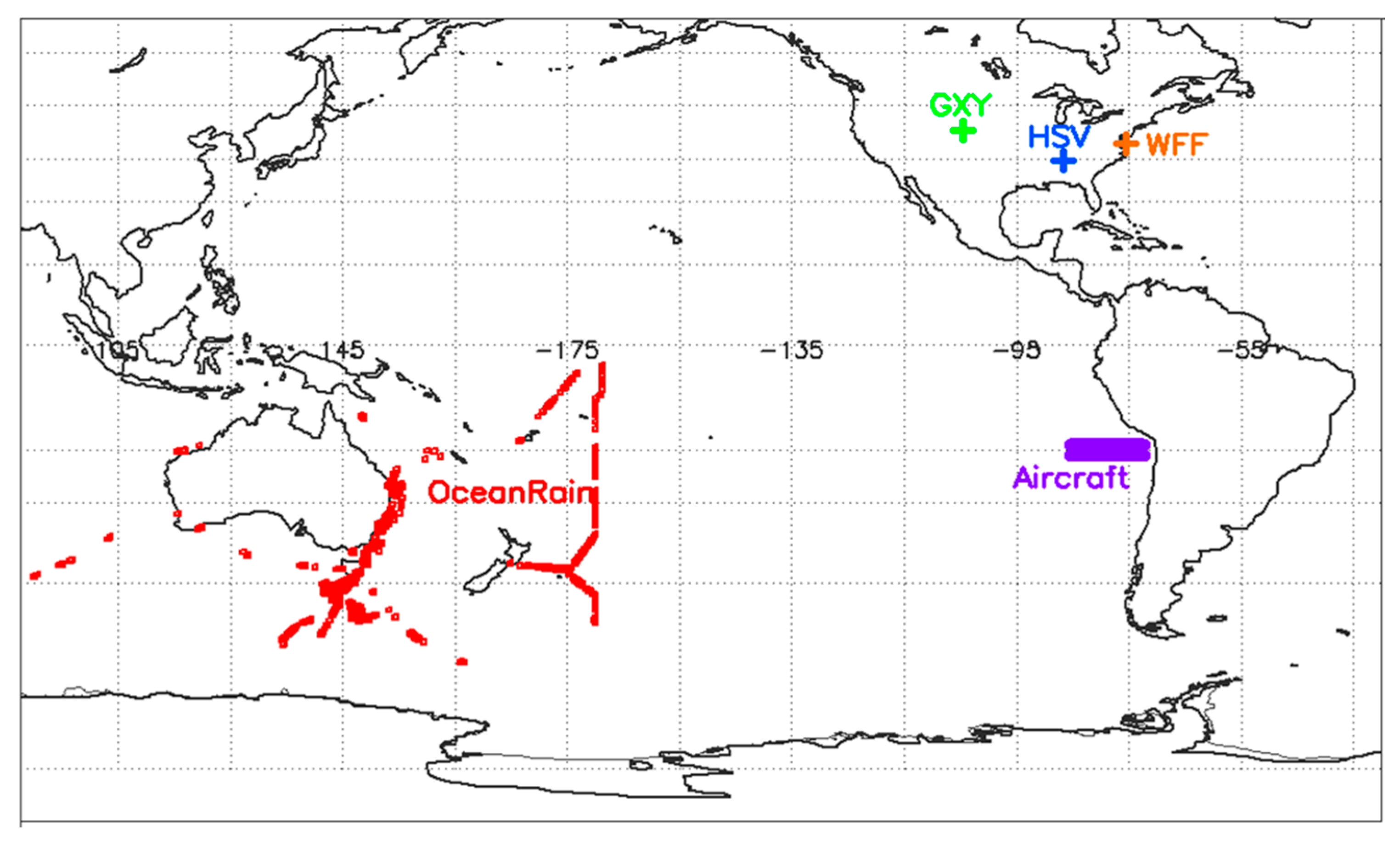
Measured DSDs from semi-arid Greeley (GXY), Colorado, USA, and sub-tropical Huntsville (HSV), Alabama, USA, are collated together to form about 2928 3-min averaged DSDs. At each site the 2DVD and MPS instruments were placed inside a 2/3-scaled DFIR (Double Fence Intercomparison Reference windshield [30]). An identical instrument suite was recently installed at the Wallops Precipitation Research Facility (henceforth WFF), to represent a mid-latitude coastal location. Since all three sites had identical instruments, the comparison between them would not have the uncertainty and other complications of using different sensors. The data quality procedures typically follow Schoenhuber et al. [7,8], with some caveats noted by [31].
(b)
The NCAR C-130 was operated off the coast of Chile [32] equipped with a ‘fast’ 1-s 2D-C probe in stratocumulus drizzle (warm rain). The total number of 1-s DSDs was 4142, all quality controlled (J. Jensen, NCAR, personal communication).
(c)
A very large (arguably the largest ever quality controlled) set of DSDs acquired over the open ocean (OceanRain) described by Klepp et al. [33] and Protat et al. [22,23].
(d)
Simulations of gamma DSDs with uncorrelated NW, Dm, and shape parameter (μ).
(e)
The outer rain bands of: (a) Category-1 Hurricane Dorian, described by Thurai et al. [34] and modeled using a cloud particle model by Bringi et al. [35], which traversed the WFF disdrometer network site for ≈8 h; (b) tropical storm Irma (<14 h) near the Huntsville site; (c) tropical depression Nate, which was very shallow at times with negligible echo above the melting layer and ‘pure’ warm rain at times (overall <16 h) near Huntsville. Figure 1 shows the locations marked as WFF and HSV. The outer rainbands were typically stratiform in nature and occurred in the down shear left quadrant. The reason for including these DSDs is because the dynamics are known to be very different from the stratiform rain produced by mesoscale convective complexes.
A global location map of the regions where data (a–c) were collected is depicted in Figure 1, and Table 1 gives some brief information relating to the type of instruments, references to the data quality, and other salient features. As can be easily seen in Figure 1, the OceanRain project with an ODM-470 optical disdrometer ‘hardened’ for shipborne deployment (sited on top of the mast, with a wind vane to orient the instrument perpendicular to the main flow) has the largest number of 1-min DSD data collected during the voyages of the Australian Research Vessel Investigator from 2016 to 2018 covering the middle-to-upper latitudes of the S hemisphere.

3. Data Analysis

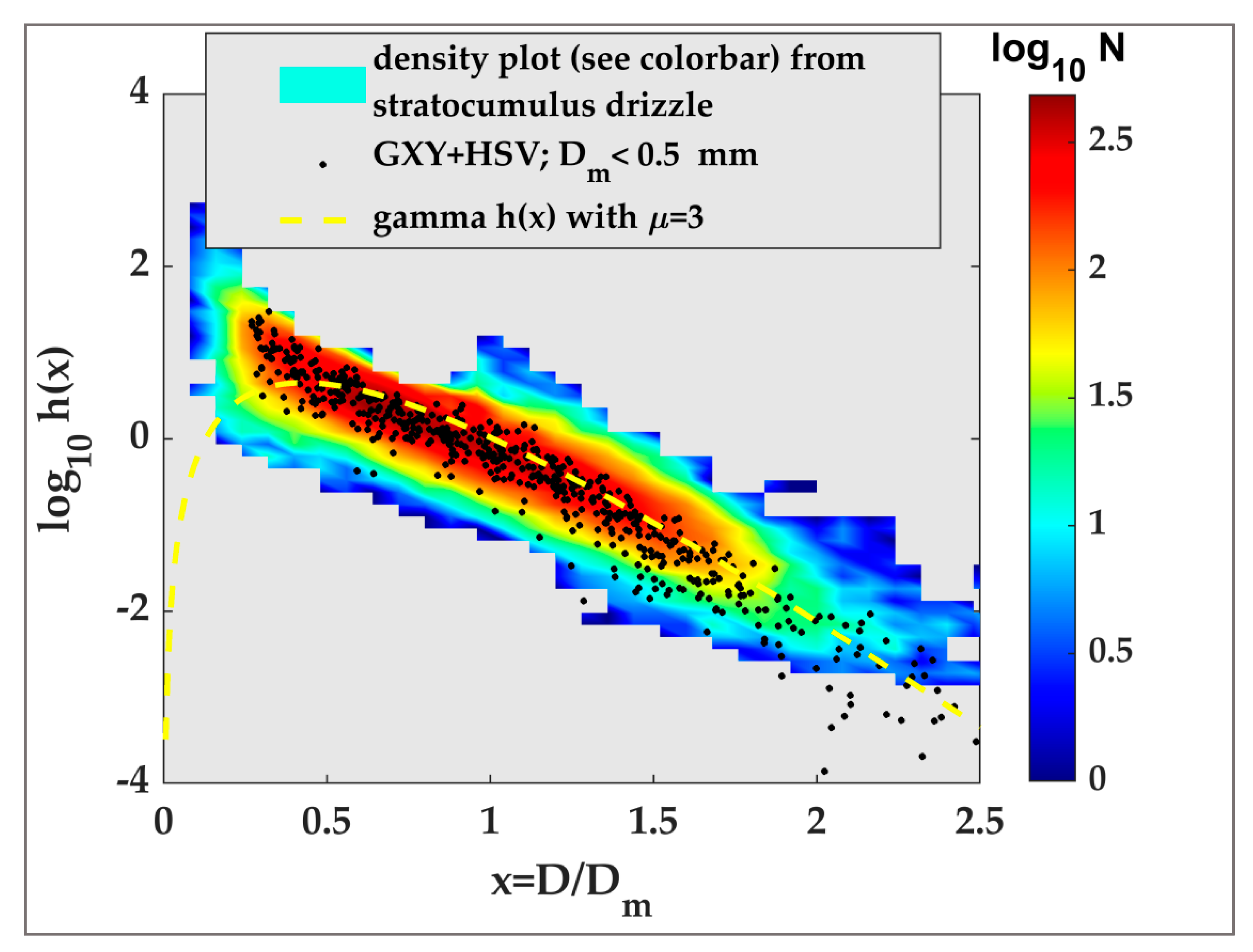
3.1. The ‘Intrinsic’ DSD Shape: Marine Stratocumulus Drizzle versus Semi-Arid and Sub-Tropical Regimes

We followed the methodology of Lee et al. [3] for the normalization of the DSDs. The reference moments chosen here are M3 and M4. Recall that h(x) is defined via N(D) = N0′ h(x), where x = D/Dm. The functional form of h(x) does not necessarily have to be specified as long as its moments are finite. A flexible form used by Thurai and Bringi [9], Protat et al. [22], and Duncan et al. [24] is the generalized gamma, which has two shape parameters. The N0′ is termed the ‘normalized’ intercept parameter and Dm, defined as M4/M3, is termed the mass-weighted mean diameter.
Figure 2 shows the double-moment normalization [3] applied to the combined Greeley (GXY) and Huntsville (HSV) datasets (scatter plot depicted as black-filled circle markers). The color contours depict the 2D histogram or density plot of h(x) using the 4412 1-s stratocumulus drizzle DSDs. The color bar shows the contours of log N. The maximum Dm of the drizzle DSDs was about 0.5 mm (see Figure 3a later). Hence, to compare the h(x) between the drizzle and the GXY-HSV data, we chose to threshold the latter at Dm = 0.5 mm for consistency.
The colored contours of the density of h(x) for the drizzle are compact and the scatter of the GXY-HSV h(x) are noted to be well-confined by the contour at N = 100, which is indicative of h(x) stability across very different rainfall regimes, e.g., [9,22]. Also shown in Figure 2 is the h(x) for the gamma model with μ = 3. The agreement is quite good for x > 0.5, below which the h(x) drops off very rapidly, whereas when two disdrometers are used, such as MPS and 2DVD, the x < 0.5 region is shaped concave up (as in [36]). The total drop concentration in the gamma model with μ = 2 to 3 can be low by an order of magnitude, which will bias, for example, the rain water content and the Ka-band specific attenuation, which are linearly related (we are referring to below cloud base, thus excluding cloud droplets). This is bound to impact the CMB algorithm, where the Ka-band reflectivity and path integrated attenuation are simulated from the attenuation-corrected Ku-band radar data.

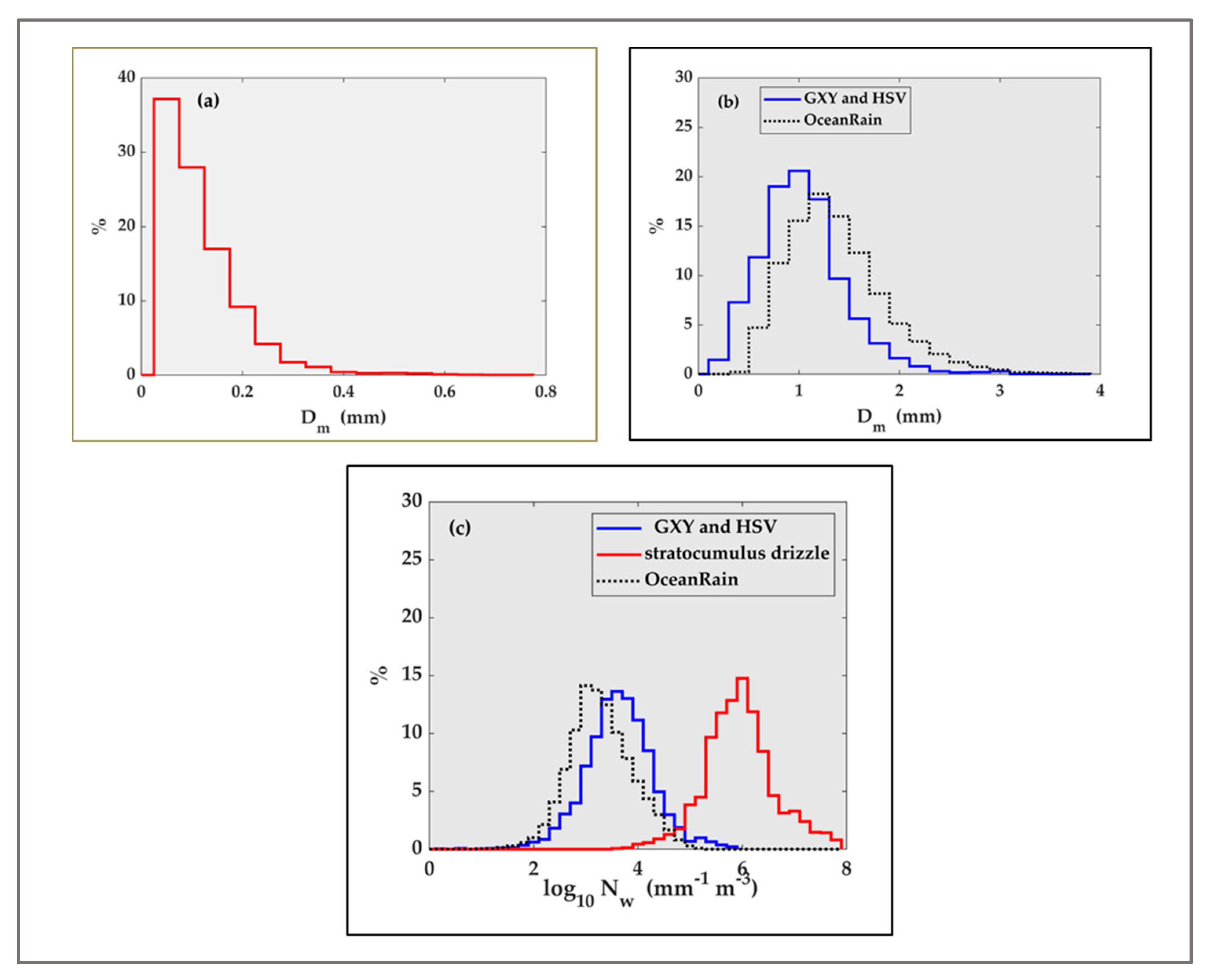
3.2. Histograms of DSD Parameters
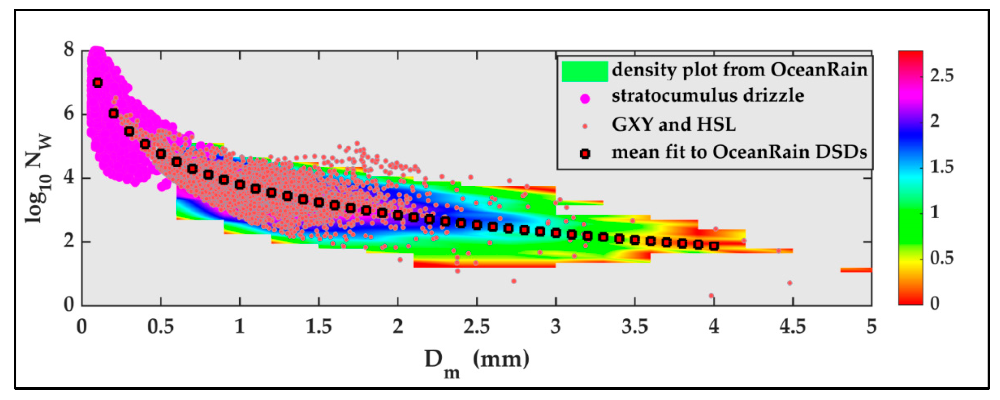
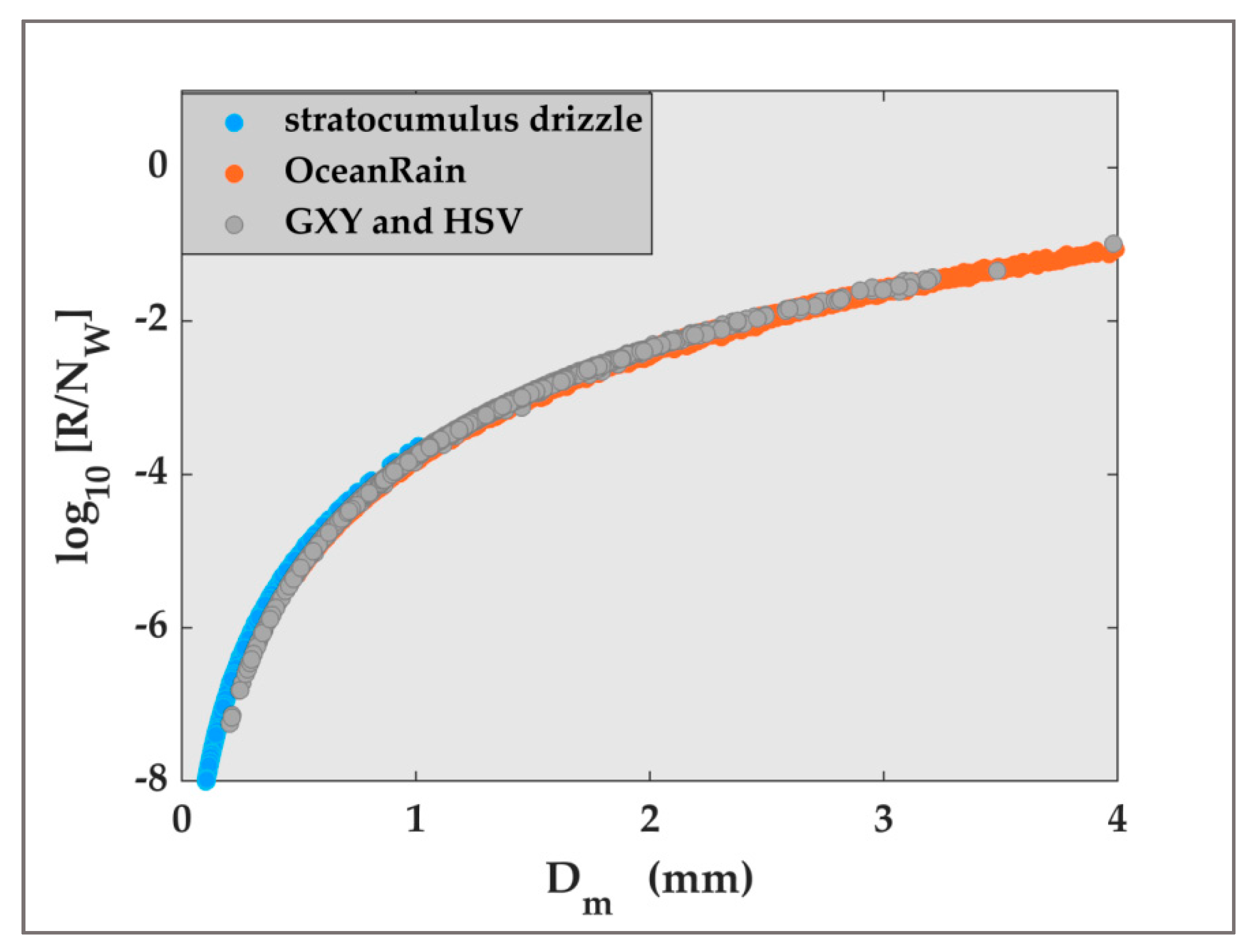
The histograms of the DSD parameters [log10 (NW); Dm] give valuable information when different rain regimes are compared. Note that these parameters can be computed for any measured DSD. Figure 3 panel (a) shows the histogram of Dm and panel (c) shows log10 NW from stratocumulus drizzle using a ‘fast’ 2D-cloud probe (on aircraft) with a 25 μm resolution. The shape o latter is quite symmetric about the mode which is high at 106 mm−1 m−3. The aircraft also had a cloud droplet probe (CDP) to measure in-cloud size spectra. The stratocumulus clouds were warm, and both cloud droplets and drizzle were present. However, the size spectra from the 2D-C probe, when compared with the droplet spectra from the CDP, showed spectral separation at sizes of about 50 μm. Hence, we have no reason to believe that the log10 NW histogram of drizzle in panel (c) is incorrect. The Dm histogram of drizzle in panel (a) is very positively skewed and of unusual shape.
Panels (b) and (c) of Figure 3 compare the histograms of Dm and log NW from overland and over ocean. The differences in the shape, mode, and width indicate that oceanic DSDs from the Southern Hemisphere high latitudes are characterized by lower concentrations of slightly bigger drops than DSDs over land. The difference in log (Nw) is consistent with the latitudinal variability observed between oceanic DSDs from the Southern Hemisphere high-latitude and from the Northern Hemisphere mid-latitude bands discussed in [22]. However, no difference was observed between the oceanic Dm in those two latitude bands. Therefore, the observed variability between the two datasets seems to be attributable to a mixture of latitudinal and land versus ocean variability.
Liao et al. [29] obtained histogram shapes and modal values very close to our GXY-HSV combined histogram. Their database had >216,000 1-min DSDs using Parsivel disdrometers from NASA Ground Validation field projects such as MC3E, IFLOODs, and Wallops, representing regimes corresponding to deep summer convection in central Oklahoma, springtime convection in Iowa, and mid-latitude coastal regimes, respectively.
It is clear that marine drizzle cannot be detected by the Ku- or Ka-band radars. However, the plot of Zku versus Dm (see Figure 4) from drizzle and GXY-HSV illustrates that perhaps the drizzle branch ‘joins’ the more intense rainfall region fairly continuously. The reflectivity of drizzle at Ku-band varies very sharply as Dm increases (the drizzle is shown as a density plot) like a nearly ‘vertical’ tower, with Dm approximately constant at around 0.2 mm, while NW increases with Zku. This feature of very tight compression generally occurs only when Zku is normalized by NW prior to plotting against Dm. The scatter plot in Figure 4 is from GXY-HSV, which shows that increasing Zku is accompanied by increasing Dm, along with much higher variability.

3.3. NW versus Dm

As discussed previously, the most important covariability (next to Dm versus R) of the DSD gamma parameters used in the CMB algorithm is between log(NW) and Dm, which enables one to choose the a priori state as well as to nudge the log(NW) in the ‘correct’ direction to minimize the cost function, as in the latest version of the CMB algorithm. Section 4 deals exclusively with this topic, so only the salient points are given here.
Figure 5 shows the log(NW) versus Dm variations derived from the ground-based, OceanRain, and airborne DSDs. A few caveats (see Table 1) of the interpretation of this figure are: (a) the varying number of data points in each rainfall regime (locations); (b) the differences in instrument types and measurement volumes and if theoretical drop fall speeds or measured values are used; (c) no classification of rain type is done, e.g., stratiform or convective rain.
In spite of these caveats, the following points can be made:
(a)
From the high resolution (25 microns) ‘fast’ 2D cloud probe aircraft DSD data, we found that the drizzle Dm is generally <0.5 mm with NW spanning at least two orders of magnitude for any given Dm;
(b)
The NW–Dm points from GXY-HSV appear to smoothly merge with the drizzle data for Dm < 0.35 mm;
(c)
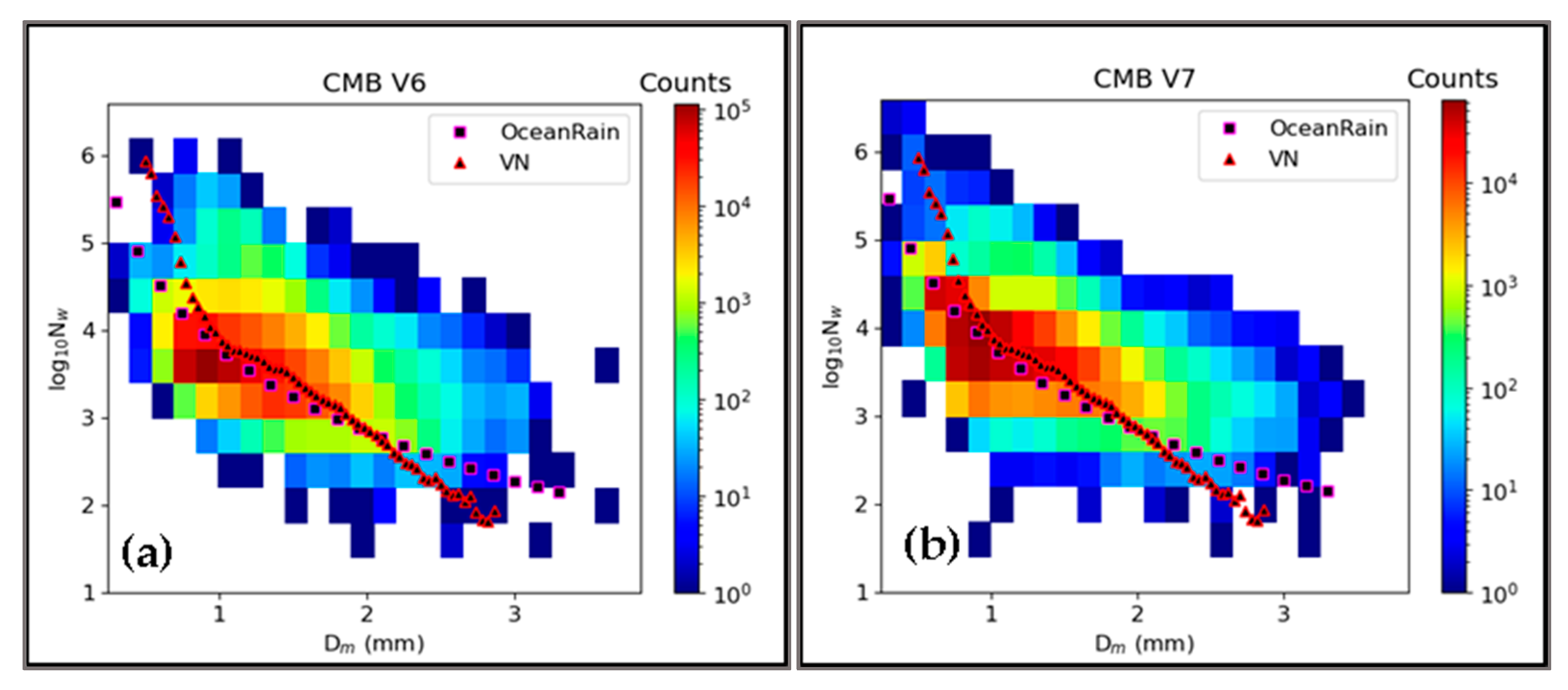
The mean power law fit from [22], from their OceanRain DSDs, shown as ‘squares’, is an excellent fit through the entire size range covered by all datasets (with the exception of drizzle; see Appendix A), despite the large variability of NW for any given Dm. This is a major finding of this paper.

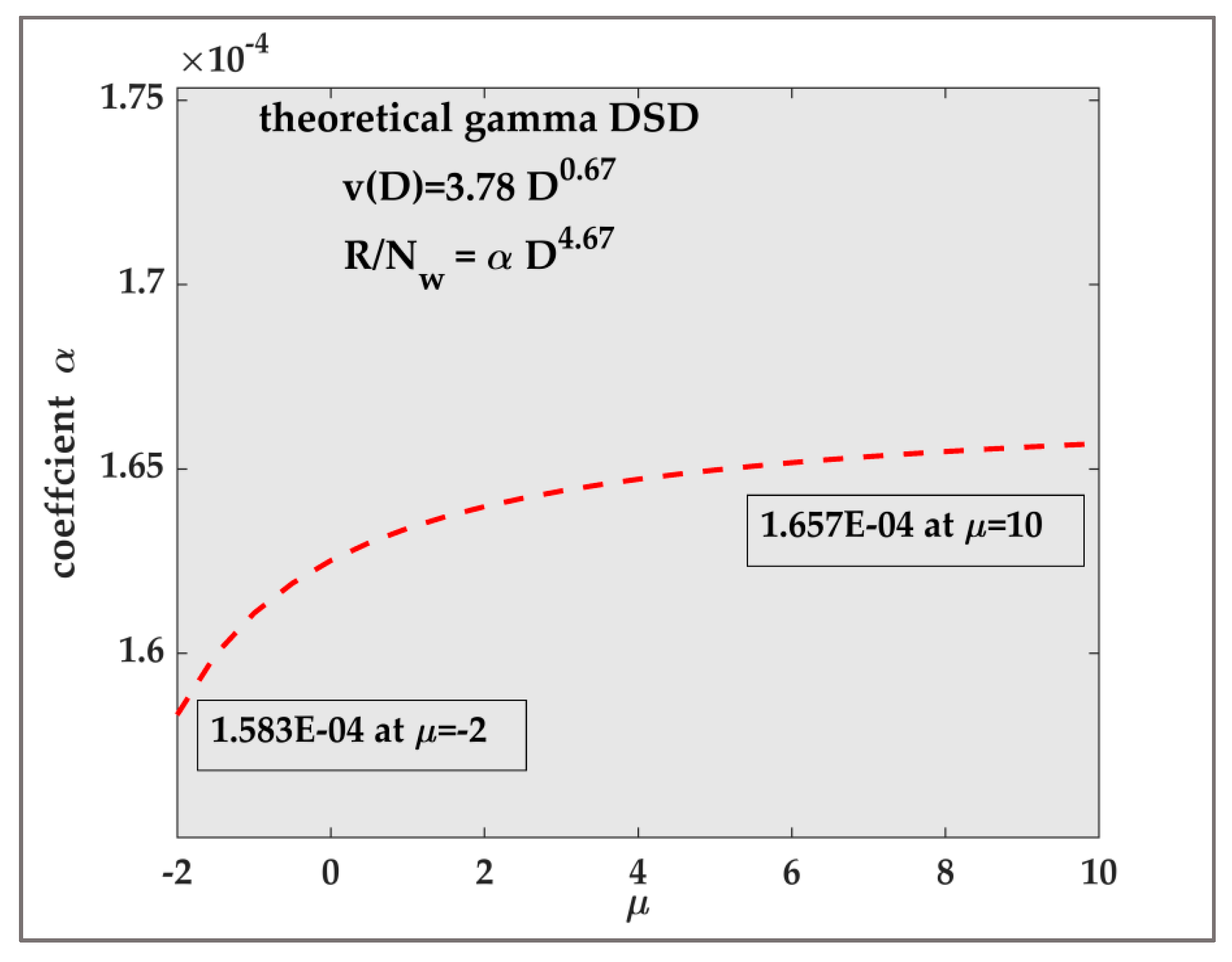
3.4. The Relationship between Rain Rate and DSD Gamma Parameters

The rain rate (R) variability is not only due to variations in the parameters that describe the parametric form of the DSD but also the intrinsic or ‘underlying’ DSD shape termed h(x), which arises as a result of the scaling normalization framework [3,4]. If the h(x) is stable across different rain types and climatologies, it forms a strong constraint that can be used in satellite (and ground-based) radar rainfall retrievals. For example, if the parametric form of h(x) is gamma, then a constant shape factor (e.g., μ = 2 to 3) defines h(x), provided the small drop truncation is negligible. If the disdrometer cannot measure the small drop end accurately, the h(x) can be stable but incorrect. In any case, NW and Dm are the two unknown DSD parameters that need to be retrieved. The ideal scenario is the selection of the number and order of the reference moments, whereby the scatter in h(x) is greatly reduced. In practice, the integral quantities that need to be estimated are R and rain water content (W) and perhaps other moments along with their error statistics. The GPM mission has adopted the Testud et al. [1] formulation (i.e., the scaled-normalized form) of the DSD.
From a theoretical (normalized) gamma model with parameters (NW, Dm, and μ) along with the simplified fall speed relation v = 3.78 D0.67 [37], where v is in ms−1 and D in mm, it follows from [1] that:
R N W = 3.78 [ 0.6 π 10 3 ] 6 4 4 ( 4 + μ ) ( μ + 4 ) Γ ( 4 + μ ) Γ ( μ + 4.67 ) [ Γ ( μ + 4 ) ] ( μ + 4.67 ) Γ ( μ + 5 ) ( μ + 4.67 ) D m 4.67
R N W = α D m 4.67
Figure 6 shows the theoretical plot of α = f(μ), showing that α varies very slowly with μ in the range of −2 to 10. Figure 7 shows the variation in R/NW versus Dm obtained by (a) simulating a gamma distribution with the parameters being uncorrelated from each other but uniformly distributed in the intervals 200 to 6 × 106 mm−1 m−3, 0 to 4 mm, and −2 to 4 for NW, Dm, and μ, respectively, and (b) using the theoretical equation with μ = 0, i.e., exponential DSD. The agreement between using (a) random gamma (i.e., with random parameters being uniform in their respective intervals) and (b) a fixed gamma with shape parameter 0 is a point to be noted. To the best of our knowledge, this point has not been made in the literature. A simple explanation is that NW cancels off in the ratio R/NW. The residual variability in R/NW is then due to (μ, Dm). However, in the random gamma simulations, there is no imposed correlation between log(NW) and Dm or R and Dm. To complete this sub-section, Figure 8 compares R/NW versus Dm from the measured DSDs from the 1-s marine stratocumulus, OceanRain, and GXY-HSV. The curves are practically identical, with differences in R/NW being of the order of <1% in log scale.

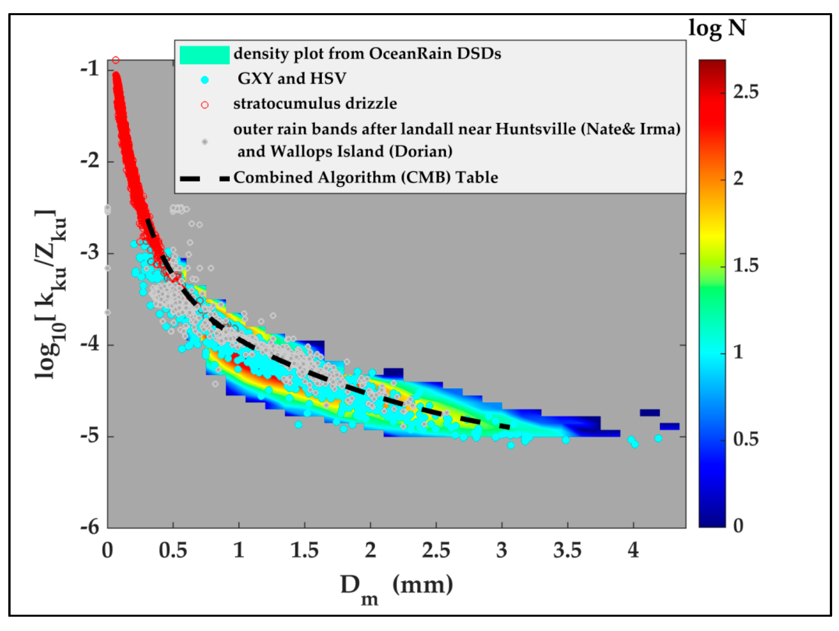
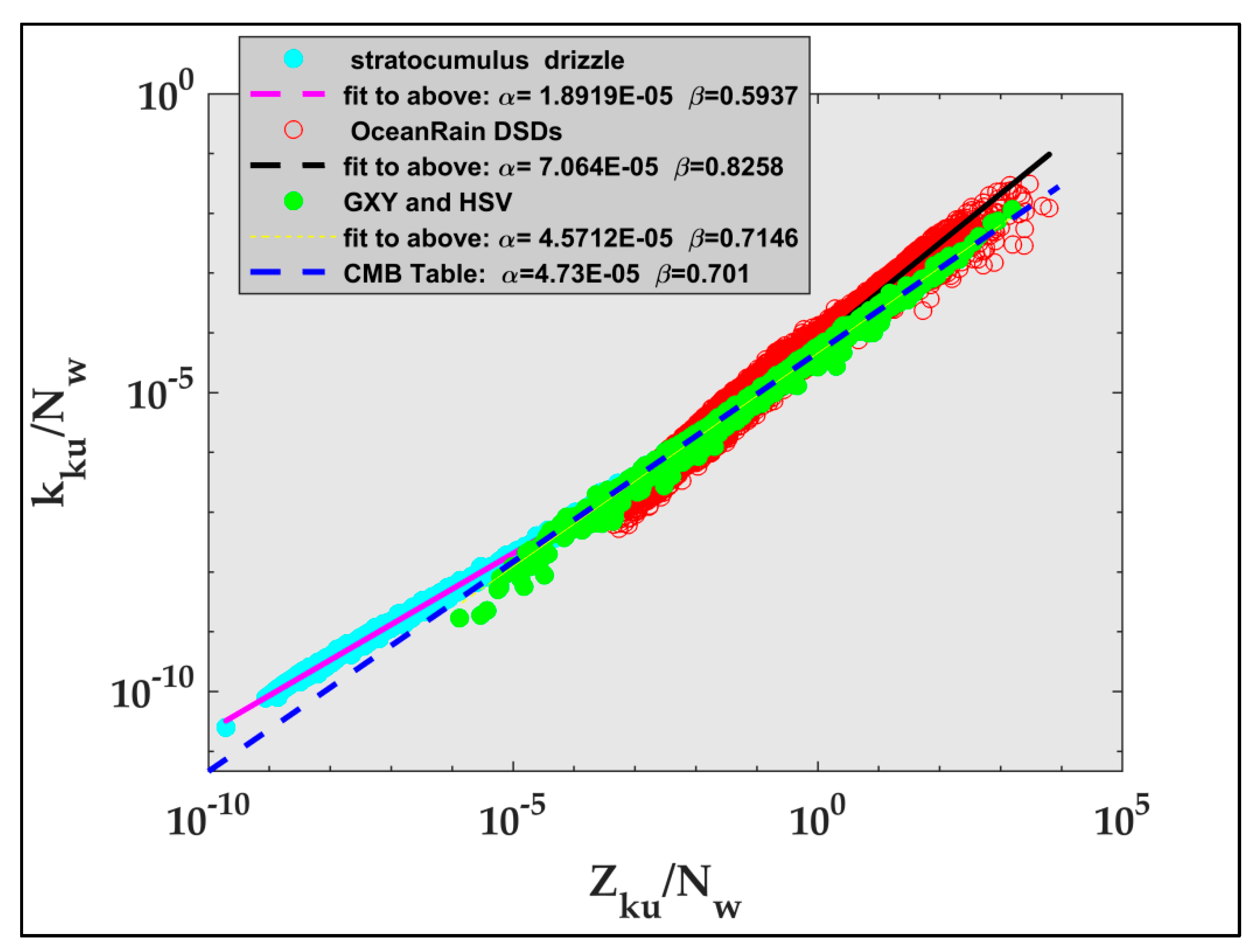
3.5. The Relation between Normalized Radar Quantities and Dm

The CMB algorithm uses measured Zku and the generalized Hitschfeld–Bordan algorithm [19], where the specific attenuation kku versus Zku relation is expressed as a power law, to derive the initial profile of Dm. In this context, Figure 9 is important as the DSD-based simulations of kku and Zku (using the T-matrix scattering code; [38]) and their ratio (from various regimes described in the legend) fall on an ‘invariant’ curve without the need for rain type classification. Note that we have added DSDs from the outer rain bands of tropical storms Nate and Irma (after landfall near Huntsville) and hurricane Dorian (as it traversed over Wallops [34,35]). These DSDs are primarily stratiform with bright-band and some embedded weak convection (in total covering > 25 h of rainfall), with Nate having the lowest R (shallow and warm rain at times). For 0.5 < Dm < 2.5 mm, their overlap with OceanRain and GXY-HSV is visually excellent. The most relevant is the excellent fit of the CMB look-up table values to the measured DSDs (black dashed line). The variability of kku/Zku for a given Dm is due to the numerator and denominator being proportional to different moments of the DSD (approximately M3 and M6).
We now turn our attention to the relation between R and radar observables, such as Zku, that have both been normalized by NW. This relation is used in the CMB retrieval algorithm, and therefore, it is important to compare the lookup tables used in the CMB with measured DSDs and our T-matrix scattering calculations. The lookup tables are based on theoretical gamma DSDs with the parameters Dm and μ being varied systematically (and NW set to 1 mm−1 m−3).
Figure 10 shows the relation between R/NW and Zku/NW for the different regimes. The straight line fits are remarkably parallel to each other. Note that a straight line fit to log(R/NW) versus log[Zku/NW] gives the slope (β) and intercept (α) of a power law of the form R = α NW(1-β) Zkuβ. It certainly appears that a single relation, with mean α = 0.0014 and mean β = 0.6514, would be appropriate for all the DSDs considered. Table 2 lists the (α, β) values, including the values for the random gamma simulated DSDs. It can be shown that there is a close relationship between NW and the parameter ε described by Iguchi et al. [39].
At Ka-band, shown in Figure 11, the relationship of normalized R with normalized Zka is bound to be affected by non-Rayleigh scattering, as indicated by the enhanced scatter for the OceanRain DSDs. Both the GXY-HSV and OceanRain show non-linear behavior in the log-log domain. The slopes vary depending on the DSD source, the stratocumulus drizzle showing the smallest β = 0.64, whereas the GXY-HSV, the random gamma, and the CMB table show that the corresponding β values are very close to 0.73. The CMB fit at Ka-band matches the observations in terms of the slope up to Ze/NW~ 1, but a more complex piecewise fitting would be required to better match the non-linearity caused by non-Rayleigh scattering.
Another important plot in the context of evaluating the current assumptions held in the CMB algorithm is k/NW vs. Ze/NW (see Figure 12 and Figure 13), which, if linear in the log-log domain, will result in (as before) k = α NW(1-β) Zeβ. The linearity between the various measured DSDs is not expected to be perfect, i.e., some non-linearity is to be expected at the drizzle end (where different moments are correlated: M6 versus M3) and at the upper end (non-Rayleigh scattering versus M3). This is confirmed in Figure 12 (for Ku-band) and Figure 13 (for Ka-band).
Table 2 and Table 3 give the coefficient α and the exponent β for the four DSD regimes, as represented by the three datasets. The CMB table values are close to the others, except for the drizzle fits. Additionally, note that the non-linearity is more evident at Ku-band (Figure 12) relative to Ka-band (Figure 13). Atlas et al. [37] showed that at Ka-band, the specific attenuation is linear with rain rate but not at lower frequencies, which would account for the non-linearity at Ku-band. The ‘best’ match at Ku-band is between the measured DSDs from GXY-HSV and the CMB table. From the radar profiling perspective, normalized k–Ze relationships are crucial for attenuation correction. The CMB lookup tables are based on a set of theoretical gamma DSDs (and not measured DSDs), yet the slope and exponent from the CMB tables are in good agreement with measured DSDs (exceptions noted above). Note also from Table 3, that the fit to random gamma-simulated DSDs is nearly identical with the CMB lookup table values.
The non-linearity of k/NW versus Ze/NW, while introducing complications in the attenuation correction algorithm, does not fundamentally change the methodology. A major source of uncertainty in the attenuation correction process is obviously NW. The large variability of NW and the NW–Dm relationships in the same (or different) climate regimes was documented in the prior section for our datasets, but these are still limited and need to be expanded to reduce uncertainties. The first results of using the research version of the CMB algorithm seem to indicate that over the Southern Ocean, the CMB algorithm starts the retrieval process with an underestimated value of NW. This could potentially explain the large discrepancies reported between different satellite products at high southern hemisphere latitudes [17].
From the plots in Figure 10, Figure 11, Figure 12 and Figure 13, a strong result, hitherto not reported in the literature, is that after normalization, the CMB tables are in very good agreement with observational data and rather surprisingly with random gamma DSDs as well. The marine drizzle DSDs cannot be detected by GPM sensors due to sensitivity limits at Ku- and Ka-bands. Furthermore, the biases and uncertainties in CMB retrievals could arise from the incorrect specification of the a priori state and how representative it is of the climatology of the retrieval regime. One useable constraint is the relation between log(NW) and Dm (see Figure 5), which on average is close to the fit from the OceanRain DSDs alone [22,23]. Notwithstanding the large spread due to different rain regimes, we have indirect evidence that NW–Dm constraints are useful, but not fully proven as of yet, in improving the retrieval of the rain rate using the CMB Algorithm.

4. Application to the CMB Algorithm

As mentioned in the previous sections, the combined algorithm employs a nudging procedure to weakly enforce NW–Dm climatological constraints in the retrievals. The reason why NW–Dm climatological relationships are useful is that even when dual-frequency observations are available (i.e., within the matched swath before June 2018 and across the entire swath after the change in the DPR pattern scanning strategy), NW and Dm cannot be uniquely and unambiguously estimated. Climatological NW–Dm information improves the estimation process by eliminating estimates inconsistent with a priori observations. The NW–Dm constraining procedure was introduced in Version 6 of the combined algorithm [25]. Specifically, the relation between NW and Dm was derived from the GPM Validation Network (VN; [40]) polarimetric radar products and implemented in the algorithm in a two-step procedure. In the first step, a radar-only retrieval is performed, assuming a nominal NW value that is independent of Dm. In the second step, the NW is nudged towards the value predicted by the VN relations for the Dm derived in step 1. Specifically, NW is updated by an increment proportional to the difference between the value predicted by the VN relation and its first step value. In V6, the procedure is applied only to stratiform rain and the nudging coefficient is determined through trial and error. The nudging is not applied to convective precipitation, as the VN NW–Dm relationships predicts NW values that tend to result in substantial underestimation of severe convection.
A two-dimensional NW–Dm histogram (or density plot) derived from one month (August 2018) of V6 data is shown in Figure 14a. The average VN and OceanRain NW–Dm relationships are also shown in the figure. As apparent in the figure, although the (color contoured) density plot of the retrieved NW–Dm exhibits an inverse relationship qualitatively similar to those derived from direct observations, there are also significant discrepancies, especially for large Dm values. Some of these discrepancies may be explained by the differences between the spatial scales of the satellite and ground products. However, notable differences exist between the VN and OceanRain fits as well. As the nudging coefficient was determined by trial and error to minimize biases with respect to the same ground reference products as those in [15], the use of the VN-based NW–Dm relationship (which is highly biased for a small Dm and less biased for a large Dm with respect to the OceanRain relationship) did not result in increased biases for Dm smaller than 0.7 mm and larger than 2.0 mm. This is also the reason the OceanRain fit (which is not used per se in the Nw adjustment) is in better agreement with the density plot of the V6 NW–Dm data than the VN relationship (which is actually used in the adjustment).
As the details of this research were still emerging at the time the NW–Dm nudging procedure was revisited in V7 of the combined algorithm, the VN NW–Dm rather than OceanRain curve (which is also consistent with the GXY-HSV dataset) was used. Nevertheless, several changes were introduced in the algorithm. Specifically, the nudging procedure was extended to convective precipitation as well. As the VN stratification by precipitation types did not result in significantly different NW–Dm curves (except for very large Dm), the same curve shape was used for both convective and stratiform. However, the convective curve was shifted upwards by log10(NW) = 0.5 relative to the stratiform curve. That is, NW was nudged towards a relationship that predicts a value of log10(NW) that is larger by 0.5 than the curve shown in Figure 14 (which is valid only for stratiform precipitation). The shift was determined by trial and error and evaluation against ground estimates. In retrospect, the OceanRain NW–Dm curve (which, as mentioned before, is consistent with the GXY-HSV dataset) is a better option, but other items requiring attention in the combined algorithm (such as the mitigation of ground clutter and uncertainties in orographic) precluded additional NW–Dm updates in V7. Nevertheless, the current NW–Dm updates resulted in an overall increase of 7% of surface rain rates over land, which appear to offset some known biases in V6, and better consistency between single and dual frequency retrievals. The V7 histogram (density plot) of retrieved NW and Dm is shown in Figure 14b. As apparent in the figure, the agreement between the combined retrievals and OceanRain is improved for the same reason mentioned in the previous paragraph. The most significant changes in the V7 NW–Dm two-dimensional histogram (density plot) relative to the V6 density plot appear to occur for Dm values around 1.0 mm and smaller. Nevertheless, the discrepancies between retrieved NW–Dm and the fit to the OceanRain data for Dm > 2.0 mm are large for both V6 and V7 and are suggestive of Non-Uniform Beam Filling (NUBF) effects that may impact both the combined retrievals and the OceanRain analysis. The reconciliation of these discrepancies is left to future studies, as it likely requires a systematic revision of the NUBF parameterizations in the combined algorithm and an extended methodology to mimic NUBF effects in the NW–Dm relation derived from the OceanRain data.

5. Discussion and Summary

Multiple studies [41,42], have shown that dual frequency space-borne radar observations are generally insufficient to unambiguously estimate rain DSDs. The inclusion of Path Integrated Attenuation (PIA) estimates from the Surface Reference Technique (SRT; [43]) improves the accuracy of NW and Dm estimates [44], but the SRT PIA estimates are not always reliable and usable in the estimation process. Similarly, the inclusion of over-ocean radiometer observations in the estimation process, although beneficial [45], does not fully address the ambiguity problem, as in some situations, the signal from the surface and cloud water cannot be reliably separated from that of rain in the radiometer observations. As a consequence, additional information, such as the inverse climatological relation between NW and Dm, is necessary to further improve the accuracy of precipitation estimates from space-borne radar observations.
Jointly, the four DSD datasets investigated in this study span a large range of normalized intercepts NW and mass-weighted mean diameters Dm. However, a unifying mean NW–Dm relation appears to exist. Specifically, a relationship between NW and Dm was derived exclusively from the OceanRain dataset. At the same time, the joint NW–Dm distributions from the OceanRain and the GXY-HSV datasets overlap significantly, which, consequently, makes the OceanRain NW–Dm relationship a good fit for the GXY-HSV dataset as well. This suggests that the OceanRain NW–Dm relationship would be an appropriate constraint for global space-borne radar-based precipitation algorithms, such as the GPM combined algorithm. A comparison between the operational NW–Dm relation used as a constraint in versions 6 and 7 of the combined algorithm and the OceanRain relation shows deficiencies in the combined relation for small drops (Dm < 1 mm) and large drops (Dm > 2 mm). However, given that the constraining procedure involves nudging coefficients that have been determined by trial and error and validated against ground precipitation products, the impact of inadequacies in the combined NW–Dm constraint is rather limited. Nevertheless, the implementation of the OceanRain relation in the combined algorithm is likely to result in more accurate precipitation estimates and a better agreement between the NW–Dm distributions estimated by the combined algorithm and the NW–Dm distributions from the three datasets investigated in this study. Other priorities in the combined algorithm, such as the mitigation of ground clutter effects, precluded the implementation of the OceanRain relation in version 7 of the combined algorithm, but it is anticipated that the OceanRain NW–Dm will be implemented in the next version of the combined algorithm.
We have devoted considerable effort to comparing the statistical relationships between the parameters of the measured gamma DSD distributions, such as NW–Dm, R/NW versus Dm, and kku/Zku versus Dm. These statistical relationships are in excellent agreement with the mean fit from other similar studies [27,29]. Figure 10, Figure 11, Figure 12 and Figure 13 showed important normalized relationships between specific attenuation and reflectivity, and R/NW versus k/Ze, which were compared to the equivalent relationships in the CMB lookup tables. Although this study has demonstrated that some improvements could be brought to the ka-band relationships to better account for non-Rayleigh scattering, the overall agreement between CMB lookup tables and the simulations from measured DSDs was excellent in terms of mean power law fit values as compared in Table 2 and Table 3. This suggests that the combined lookup tables [15] are not a major source of uncertainty in the combined estimates, which is an important finding of this paper (which we believe has not been reported in other studies). It appears that the limited and hard to untangle amount of information in the observations along with other sources of uncertainties such as multiple scattering and non-uniform beam filling effects are the main causes of random and systematic errors in the combined precipitation estimates.

Author Contributions

Conceptualization, V.B. and M.G.; Methodology, Investigation, and Formal Analysis, V.B., M.G., A.P., and M.T.; Data Curation, C.K. and A.P.; Writing—Original Draft Preparation, V.B. and M.G.; Writing—Review and Editing, V.B., M.G., M.T., and A.P.; Supervision, V.B. All authors have read and agreed to the published version of the manuscript.

Funding

V.B. and M.T. were funded by the NASA Atmospheric Dynamics program via Grant Award Number 80NSSC20K0893. M.G. was supported by the NASA Precipitation Measurement Mission program via grant 80NSSC19K0674.

Data Availability Statement

Data can be made available upon request to any of the authors.

Acknowledgments

We wish to thank J. Vivekanandan and J. Jensen from NCAR for supplying quality-controlled aircraft-installed 2D-C 1-s data and G-J Huang for assistance with data processing of the aircraft data.

Conflicts of Interest

The authors declare no conflict of interest. The funders had no role in the design of this study; in the collection, analyses, or interpretation of its data; in the writing of this manuscript, and in the decision to publish these results.

Appendix A. NW versus Dm Fitted Curve

Figure 5 shows that the power-law fit from [22] was a good overall representation of the variation of NW with Dm for all datasets for the entire range, despite the large spread, e.g., in NW for any given Dm. To quantify this spread, we consider here the differences between the NW from the DSDs and from the power law fit in [22] using logarithmic transformation. If we denote NW and Dm from the DSDs as NW(measured) and Dm(measured), then:
log 10 N W = log 10 N W measured   log 10 N W fit
where:
N W fit = 6383.8   (   D m measured ) 3.19
Histograms of log 10 N W for the GXY-HSV dataset and the OceanRain dataset are shown in panel (a) of Figure A1, in green and red, respectively. Since the two histograms resemble a Gaussian-like distribution, a non-linear least-squares fit to a function with four unknown parameters, p0, p1, p2, and p3, was computed for each of the histograms. The function, denoted as f(x), used here is the following:
f ( x ) = p 0 e v 2 2 +   p 3
where:
v = x     p 1 p 2
In Equations (A3) and (A4), p0 will represent the maximum fitted value of the histograms, p1 the mode (position) of the histograms, p2 the standard deviation, and p3 any offsets connected with the histograms. Values of the fitted parameters are given in Table A1.
The fitted curve for the OceanRain Data shows somewhat lower value for p2 (i.e., narrower) and higher value for p0 (taller) than for the GXY-HSV; furthermore, it has an offset p3 very close to zero. This is to be expected since the power-law fit given in Equation (A2) was originally done for the OceanRain datasets. Both have a p1 close to zero, indicating that there is very little systematic bias. The overall conclusion here is that Equation (A2) is an excellent representation for the mean variation for both datasets, but that the GXY-HSV curve shows more spread. Note that the NW versus Dm also has a dependence on rain type, as shown for example in [46], where stratiform and convective rain were shown to be separated by a clear demarcation line. Hence, one can expect further improvement if the two rain types are considered separately.
For the drizzle dataset, however, it was found that Equation (A2) was not a good representation of the NW–Dm variation; the blue curves in panel (b) of Figure A1 show this clearly. A very clear bias is seen, having the mode of log 10 N W at ~−0.85.
Figure A1. (a) Histograms of log 10 N W   for the GXY-HSV (green) and OceanRain (rain) datasets, and their fitted curves; (b) the same as (a) but with drizzle histograms included (blue).
Remotesensing 13 02412 g0a1
Table A1. Values of the parameters fitted to the histograms in Figure A1a.
Fitted ParametersFitted Values for GXY-HSV DatasetFitted Values for OceanRain Dataset
p08.311.8
p1−0.060.07
p20.4460.342
p30.194−0.007

References

  1. Testud, J.; Oury, S.; Black, R.A.; Amayenc, P.; Dou, X. The concept of “normalized”distribution to describe raindrop spectra: A tool for cloud physics and cloud remote sensing. J. Appl. Meteorol. 2001, 40, 1118–1140. [Google Scholar] [CrossRef]
  2. Bringi, V.N.; Huang, G.; Chandrasekar, V.; Gorgucci, E. A methodology for estimating the parameters of a gamma raindrop size distribution model from polarimetric radar data: Application to a squall-line event from the TRMM/Brazil campaign. J. Atmos. Ocean. Technol. 2002, 19, 633–645. [Google Scholar] [CrossRef] [Green Version]
  3. Lee, G.; Zawadzki, I.; Szyrmer, W.; Sempere-Torres, D.; Uijlenhoet, R. A general approach to double-moment normalization of drop size distributions. J. Appl. Meteorol. 2004, 43, 264–281. [Google Scholar] [CrossRef] [Green Version]
  4. Morrison, H.; Kumjian, M.R.; Martinkus, C.P.; Prat, O.P.; Van Lier-Walqui, M. A general N-moment normalization method for deriving raindrop size distribution scaling relationships. J. Appl. Meteorol. Climatol. 2019, 58, 247–267. [Google Scholar] [CrossRef]
  5. Ulbrich, C.W. Natural variations in the analytical form of the raindrop size distribution. J. Clim. Appl. Meteorol. 1983, 22, 1764–1775. [Google Scholar] [CrossRef] [Green Version]
  6. Baumgardner, D.; Kok, G.; Dawson, W.; O’Connor, D.; Newton, R. A new ground-based precipitation spectrometer: The Meteorological Particle Sensor (MPS). In Proceedings of the 11th Conference on Cloud Physics, Ogden, UT, USA, 2–3 June 2002. Paper 8.6. [Google Scholar]
  7. Schoenhuber, M.; Lammer, G.; Randeu, W.L. One decade of imaging precipitation measurement by 2D-video-distrometer. Adv. Geosci. 2007, 10, 85–90. [Google Scholar] [CrossRef] [Green Version]
  8. Schönhuber, M.; Lammer, G.; Randeu, W.L. The 2D-Video-Distrometer. In Precipitation: Advances in Measurement, Estimation and Prediction; Michaelides, S., Ed.; Springer: Berlin/Heidelberg, Germany, 2008; pp. 3–31. ISBN 978-3-540-77654-3. [Google Scholar]
  9. Thurai, M.; Bringi, V.N. Application of the generalized gamma model to represent the full rain drop size distribution spectra. J. Appl. Meteorol. Climatol. 2018, 57, 1197–1210. [Google Scholar] [CrossRef]
  10. Thurai, M.; Bringi, V.; Gatlin, P.N.; Petersen, W.A.; Wingo, M.T. Measurements and modeling of the full rain drop size distribution. Atmosphere 2019, 10, 39. [Google Scholar] [CrossRef] [Green Version]
  11. Williams, C.R.; Kruger, A.; Gage, K.S.; Tokay, A.; Cifelli, R.; Krajewski, W.F.; Kummerow, C. Comparison of simultaneous rain drop size distributions estimated from two surface disdromters and a UHF profiler. Geophys. Res. Lett. 2000, 27, 1763–1766. [Google Scholar] [CrossRef] [Green Version]
  12. Kozu, T.; Iguchi, T.; Shimomai, T.; Kashiwagi, N. Raindrop size distribution modeling from a statistical rain parameter relation and its application to the TRMM precipitation radar rain retrieval algorithm. J. Appl. Meteorol. Climatol. 2009, 48, 716–724. [Google Scholar] [CrossRef]
  13. Bringi, V.N.; Chandrasekar, V.; Hubbert, J.; Gorgucci, E.; Randeu, W.L.; Schoenhuber, M. Raindrop size distribution in different climatic regimes from disdrometer and dual-polarized radar analysis. J. Atmos. Sci. 2003, 60, 354–365. [Google Scholar] [CrossRef]
  14. Petersen, W.A.; Kirstetter, P.E.; Wang, J.; Wolff, D.B.; Tokay, A. The GPM Ground Validation Program. In Satellite Precipitation Measurement; Springer: Cham, Germany, 2020; pp. 471–502. [Google Scholar]
  15. Grecu, M.; Olson, W.S.; Munchak, S.J.; Ringerud, S.; Liao, L.; Haddad, Z.; Kelley, B.L.; McLaughlin, S.F. The GPM Combined Algorithm. J. Atmos. Ocean. Technol. 2016, 33, 2225–2245. [Google Scholar] [CrossRef]
  16. Huffman, G.J.; Bolvin, D.T.; Braithwaite, D.; Hsu, K.; Joyce, R.; Xie, P.; Yoo, S.H. NASA global precipitation measurement (GPM) integrated multi-satellite retrievals for GPM (IMERG). In Algorithm Theoretical Basis Document (ATBD); 2019; Version 6; p. 39. Available online: https://gpm.nasa.gov/sites/default/files/document_files/IMERG_ATBD_V06.pdf (accessed on 19 June 2021).
  17. Skofronick-Jackson, G.; Petersen, W.A.; Berg, W.; Kidd, C.; Stocker, E.F.; Kirschbaum, D.B.; Kakar, R.; Braun, S.A.; Huffman, G.J.; Iguchi, T.; et al. The Global Precipitation Measurement (GPM) mission for science and society. Bull. Am. Meteorol. Soc. 2017, 98, 1679–1695. [Google Scholar] [CrossRef] [PubMed]
  18. Kidd, C.; Becker, A.; Huffman, G.J.; Muller, C.L.; Joe, P.; Skofronick-Jackson, G.; Kirschbaum, D.B. So, how much of the earth’s surface is covered by rain gauges? Bull. Am. Meteorol. Soc. 2017, 98, 69–78. [Google Scholar] [CrossRef]
  19. Hitschfeld, W.; Bordan, J. Errors inherent in the radar measurement of rainfall at attenuating wavelengths. J. Meteorol. 1954, 11, 58–67. [Google Scholar] [CrossRef] [Green Version]
  20. Bringi, V.N.; Tolstoy, L.; Thurai, M.; Petersen, W.A. Estimation of spatial correlation of rain drop size distribution parameters and rain rate using NASA’s S-band polarimetric radar and 2D-video disdrometer network: Two case studies from MC3E. J. Hydrometeor. 2015, 16, 1207–1221. [Google Scholar] [CrossRef] [Green Version]
  21. Viltard, N.; Kummerow, C.; Olson, W.S.; Hong, Y. Combined use of the radar and radiometer of TRMM to estimate the influence of drop size distribution on rain retrievals. J. Appl. Meteorol. 2000, 39, 2103–2114. [Google Scholar] [CrossRef]
  22. Protat, A.; Klepp, C.; Louf, V.; Petersen, W.A.; Alexander, S.P. The latitudinal variability of oceanic rainfall properties and its implication for satellite retrievals: 1. Drop size distribution properties. J. Geophys. Res. Atmos. 2019, 124, 13291–13311. [Google Scholar] [CrossRef]
  23. Protat, A.; Klepp, C.; Louf, V.; Petersen, W.A.; Alexander, S.P.; Barros, A.; Leinonen, J.; Mace, G.G. The latitudinal variability of oceanic rainfall properties and its implication for satellite retrievals: 2. The relationships between radar observables and drop size distribution parameters. J. Geophys. Res. Atmos. 2019, 124, 13312–13324. [Google Scholar] [CrossRef]
  24. Duncan, D.I.; Eriksson, P.; Pfreundschuh, S.; Klepp, C.; Jones, D.C. On the distinctiveness of observed oceanic raindrop distributions. Atmos. Chem. Phys. 2019, 19, 6969–6984. [Google Scholar]
  25. Olson, W.S.; Masunaga, H.; GPM Combined Radar-Radiometer Algorithm Team. GPM Combined Radar-Radiometer Precipitation Algorithm Theoretical Basis Document (Version 4); NASA: Washington, DC, USA, 2019.
  26. Gatlin, P.N.; Petersen, W.A.; Pippitt, J.L.; Berendes, T.A.; Wolff, D.B.; Tokay, A. The GPM validation network and evaluation of satellite-based retrievals of the rain drop size distribution. Atmosphere 2020, 11, 1010. [Google Scholar] [CrossRef]
  27. Chase, R.J.; Nesbitt, S.W.; McFarquhar, G.M. Evaluation of the Microphysical Assumptions within GPM-DPR Using ground-based observations of rain and snow. Atmosphere 2020, 11, 619. [Google Scholar] [CrossRef]
  28. Tokay, A.; D’Adderio, L.P.; Wolff, D.B.; Petersen, W.A. Development and evaluation of the raindrop size distribution parameters for the NASA global precipitation measurement mission ground validation program. J. Atmos. Ocean. Technol. 2020, 37, 115–128. [Google Scholar] [CrossRef]
  29. Liao, L.; Meneghini, R.; Iguchi, T.; Tokay, A. Characteristics of DSD bulk parameters: Implication for radar rain retrieval. Atmosphere 2020, 11, 670. [Google Scholar] [CrossRef]
  30. Rasmussen, R.; Baker, B.; Kochendorfer, J.; Meyers, T.; Landolt, S.; Fischer, A.P.; Black, J.; Thériault, J.M.; Kucera, P.; Gochis, D.; et al. How well are we measuring snow: The NOAA/FAA/NCAR winter precipitation test bed. Bull. Am. Meteorol. Soc. 2012, 93, 811–829. [Google Scholar] [CrossRef] [Green Version]
  31. Larsen, M.; Schönhuber, M. Identification and characterization of an anomaly in 2-dimensional video disdrometer data. Atmosphere 2018, 9, 315. [Google Scholar] [CrossRef] [Green Version]
  32. Wood, R.; Mechoso, C.R.; Bretherton, C.S.; Weller, R.A.; Huebert, B.; Straneo, F.; Albrecht, B.A.; Coe, H.; Allen, G.; Vaughan, G.; et al. The VAMOS Ocean-cloud-atmosphere-land study regional experiment (VOCALS-REx): Goals, platforms, and field operations. Atmos. Chem. Phys. 2011, 11, 627–654. [Google Scholar] [CrossRef] [Green Version]
  33. Klepp, C.; Michel, S.; Protat, A.; Burdanowitz, J.; Albern, N.; Kähnert, M.; Dahl, A.; Louf, V.; Bakan, S.; Buehler, S.A. OceanRAIN, a new in-situ shipboard global ocean surface-reference dataset of all water cycle components. Sci. Data 2018, 5, 180122. [Google Scholar] [CrossRef]
  34. Thurai, M.; Bringi, V.N.; Wolff, D.B.; Marks, D.A.; Pabla, C.S. Drop size distribution measurements in outer rainbands of hurricane dorian at the NASA wallops precipitation-research facility. Atmosphere 2020, 11, 578. [Google Scholar] [CrossRef]
  35. Bringi, V.; Seifert, A.; Wu, W.; Thurai, M.; Huang, G.-J.; Siewert, C. Hurricane dorian outer rain band observations and 1D particle model simulations: A case study. Atmosphere 2020, 11, 879. [Google Scholar] [CrossRef]
  36. Abel, S.J.; Boutle, I.A. An improved representation of the rain size spectra for single-moment microphysics schemes. Quart. J. R. Meteorol. Soc. 2012, 138, 2151–2162. [Google Scholar] [CrossRef]
  37. Atlas, D.; Ulbrich, C.W. Path- and area-integrated rainfall measurement by microwave attenuation in the 1–3 cm band. J. Appl. Meteorol. Climatol. 1977, 16, 1322–1331. [Google Scholar] [CrossRef] [Green Version]
  38. Barber, P.; Yeh, C. Scattering of electromagnetic waves by arbitrarily shaped dielectric bodies. Appl. Opt. 1975, 14, 2864–2872. [Google Scholar] [CrossRef]
  39. Iguchi, T.; Kozu, T.; Meneghini, R.; Awaka, J.; Okamoto, K. Rain-profiling algorithm for the TRMM precipitation radar. J. Appl. Meteorol. 2000, 39, 2038–2052. [Google Scholar] [CrossRef]
  40. Schwaller, M.R.; Morris, K.R. A ground validation network for the global precipitation measurement mission. J. Atmos. Ocean. Technol. 2011, 28, 301–319. [Google Scholar] [CrossRef] [Green Version]
  41. Meneghini, R.; Kozu, T.; Kumagai, H.; Boncyk, W.C. A study of rain estimation methods from space using dual-wavelength radar measurements at near-nadir incidence over ocean. J. Atmos. Ocean. Technol. 1992, 9, 364–382. [Google Scholar] [CrossRef] [Green Version]
  42. Haddad, Z.S.; Meagher, J.P.; Durden, S.L.; Smith, E.A.; Im, E. Drop size ambiguities in the retrieval of precipitation profiles from dual-frequency radar measurements. J. Atmos. Sci. 2006, 63, 204–217. [Google Scholar] [CrossRef] [Green Version]
  43. Meneghini, R.; Iguchi, T.; Kozu, T.; Liao, L.; Okamoto, K.; Jones, J.A.; Kwiatkowski, J. Use of the surface reference technique for path attenuation estimates from the TRMM precipitation radar. J. Appl. Meteorol. 2000, 39, 2053–2070. [Google Scholar] [CrossRef]
  44. Ferreira, F.; Amayenc, P.; Oury, S.; Testud, J. Study and tests of improved rain estimates from the TRMM precipitation radar. J. Appl. Meteorol. 2001, 40, 1878–1899. [Google Scholar] [CrossRef]
  45. Grecu, M.; Anagnostou, E.N. Use of passive microwave observations in a radar rainfall-profiling algorithm. J. Appl. Meteorol. 2002, 41, 702–715. [Google Scholar] [CrossRef]
  46. Thurai, M.; Bringi, V.; Wolff, D.; Marks, D.; Pabla, C. Testing the drop-size distribution-based separation of stratiform and convective rain using radar and disdrometer data from a mid-latitude coastal region. Atmosphere 2021, 12, 392. [Google Scholar] [CrossRef]
Figure 1. Locations of sites where MPS and 2DVD were deployed for Ground Validation. The purple rectangle depicts the region penetrated by the C-130. The red lines depict the tracks of the R/V Investigator in 2016 and 2018.
Remotesensing 13 02412 g001
Figure 2. Density plot of h(x) from stratocumulus drizzle with number of occurrences given by the color bar in contours of log N. The GXY-HSV data are pooled together for Dm < 0.5 mm and shown as black points. The dashed yellow line is the h(x) for the gamma model with μ = 3.
Remotesensing 13 02412 g002
Figure 3. Relative frequency histograms of (a) Dm from stratocumulus drizzle, (b) same as (a) but from OceanRain and pooled DSDs from GXY-HSV, and (c) histograms of log10 (NW) from OceanRain and pooled DSDs and from stratocumulus drizzle (red line).
Remotesensing 13 02412 g003
Figure 4. Scatterplot of the reflectivity at the Ku-band versus Dm from stratocumulus drizzle (density-plot in color) and from all DSDs from GXY-HSV (blue points).
Remotesensing 13 02412 g004
Figure 5. Scatterplot of log10 (NW) versus Dm from three regimes described in the legend. The contoured density plot (refer to color bar) is from OceanRain. The mean fit to OceanRain is NW = 6383.8 Dm−3.19, where NW is in mm−1 m−3 shown as red-filled black squares. The GXY- and HSV-based points are shown in light red and those from stratocumulus DSDs are shown in magenta.
Remotesensing 13 02412 g005
Figure 6. The coefficient α versus shape factor μ for a theoretical gamma with fall speed power law v(D) in m s−1, D in mm, R in mm h−1, and NW in mm−1 m−3. Values of α are given within textboxes for μ = −2 and μ = 10.
Remotesensing 13 02412 g006
Figure 7. Rain rate (in mm h−1) normalized by NW (in mm−1 m−3) versus Dm (in mm). We compare random gamma DSDs with the theoretical result in Equation (1) with μ = 0.
Remotesensing 13 02412 g007
Figure 8. As in Figure 7, except DSDs from stratocumulus drizzle, OceanRain, and GXY-HSV.
Remotesensing 13 02412 g008
Figure 9. Ku-band-specific attenuation (kku in dB km−1) normalized by Ku-band reflectivity (Zku in mm6 m−3) versus Dm (in mm), from OceanRain DSDs, GXY-HSV DSDs, DSDs from the outer bands of Tropical Storm Irma and Tropical Depression Nate, as well as category-1 Hurricane Dorian, compared with those from the combined algorithm (CMB).
Remotesensing 13 02412 g009
Figure 10. Variation of the rain rate (R in mm h−1) normalized by NW (in mm−1 m−3) versus Ku-band reflectivity (Zku, in mm6 m−3). See legend, which lists the regimes.
Remotesensing 13 02412 g010
Figure 11. As in Figure 10, but for Ka-band.
Remotesensing 13 02412 g011
Figure 12. Variation of Ku-band specific attenuation (kku in dB km−1) normalized by NW (mm−1 m−3) versus Ku-band reflectivity (Zku, in mm6 m−3) normalized by NW. See legend, which lists the regimes.
Remotesensing 13 02412 g012
Figure 13. As in Figure 12 but for Ka-band.
Remotesensing 13 02412 g013
Figure 14. Two-dimensional histogram (or density plot) of joint (Nw, Dm) variables derived using version 6 (V6; panel a) and version 7 (V7; panel b) of the combined algorithm. Superimposed are the mean NW–Dm derived from the Validation Network (VN) and used to constrain the retrievals in V6 and V7 (symbolized with triangles) and the fit to OceanRain NW–Dm data (symbolized with squares).
Remotesensing 13 02412 g014
Table 1. Brief summary of the ground-based/OceanRain and C-130 instrumentation.
DatasetInstrumentsNumber of DSDsLocation
Ground-based
(green, blue, and orange ‘+’ marks in Figure 1)
i.
Meteorological Particle Spectrometer (MPS)
ii.
2D Video Disdrometer (2DVD)
A total of 2928 3-min ‘complete’ DSDsThree fixed locations
i.
Greeley, Colorado (six months in Spring-summer in 2015 under the CSU-CHILL radar coverage (Bringi et al. 2020)
ii.
Huntsville, Alabama (2016–current)
iii.
Wallops, Virginia (installed on 1 August 2019)
C-130 penetrations in stratocumulus drizzle off the coast of Chile (purple area in Figure 1)‘fast’ 2D-cloud probe (25 micron resolution)1-s data: 4412 DSDs1.4 km altitude, off the coast of Chile in stratocumulus drizzle.
Open ocean (shown as red squares in Figure 1)ODM 470 optical disdrometer1-min DSDs: 14,213Ocean regions surrounding Australia plus south-west Pacific.
Outer rain bands * (blue and orange ‘+’ marks in Figure 1)
i.
MPS
ii.
2DVD
A total of 1403
3-min ‘complete’ DSDs
Two fixed locations
i.
Huntsville, Alabama
ii.
Wallops, Virginia
* Tropical Depression Nate over HSV, Tropical Depression Irma over HSV and category 1 Hurricane over WFF.
Table 2. Fitted coefficient α and the exponent β, corresponding to Figure 10 and Figure 11.
DSD SourceFigure 10: R = α NW(1-β) ZkuβFigure 11: R = α NW(1-β) Zkaβ
Stratocumulus drizzleα = 0.0015β = 0.6423α = 0.0014β = 0.6412
OceanRainα = 0.0012β = 0.633α = 0.0017β = 0.7339
GXY-HSVα = 0.0015β = 0.664α = 0.0018β = 0.7336
CMB Tableα = 0.00143β = 0.666α =0.00219β = 0.727
Table 3. Fitted coefficient α and the exponent β, corresponding to Figure 12 and Figure 13.
DSD SourceFigure 12: kKu = α NW(1-β) ZKuβFigure 13: kKa = α NW(1-β) ZKaβ
Stratocumulus drizzleα = 1.89 × 10⁻⁵β = 0.5937α = 1.4 × 10⁻⁴β = 0.6
OceanRainα = 7.064 × 10⁻⁵β = 0.8258α = 7.0 × 10⁻⁴β = 0.715
GXY-HSVα = 4.57 × 10⁻⁵β = 0.7146α = 4.36 × 10⁻⁴β = 0.769
CMB Tableα = 4.73 × 10⁻⁵β = 0.701α =5.29 × 10⁻⁴β = 0.749
Random Gammaα = 4.55 × 10⁻⁵β = 0.721α =5.36 × 10⁻⁴β = 0.768
Publisher’s Note: MDPI stays neutral with regard to jurisdictional claims in published maps and institutional affiliations.

